Abstract
With the growing global demand for renewable energy, the pump as turbine (PAT) exhibits significant potential in the micro-hydropower sector. To reveal its internal unsteady flow characteristics and energy loss mechanisms, this study analyzes the internal flow field of an ultra-low specific speed pump as turbine (USSPAT) by employing a combined approach of entropy generation theory and dynamic mode decomposition (DMD). The results indicate that the outlet pressure pulsation characteristics are highly dependent on the flow rate. Under low flow rate conditions, pulsations are dominated by low-frequency vortex bands induced by rotor-stator interaction (RSI), whereas at high flow rates, the blade passing frequency (BPF) becomes the absolute dominant frequency. Energy losses within the PAT are primarily composed of turbulent and wall dissipation, concentrated in the impeller and volute, particularly at the impeller inlet, outlet, and near the volute tongue. DMD reveals that the flow field is governed by a series of stable modes with near-zero growth rates, whose frequencies are the shaft frequency (25 Hz) and its harmonics (50 Hz, 75 Hz, 100 Hz). These low-frequency modes, driven by RSI, contain the majority of the fluctuation energy. Therefore, this study confirms that RSI between the impeller and the volute is the root cause of the dominant pressure pulsations and periodic energy losses. This provides crucial theoretical and data-driven guidance for the design optimization, efficient operation, and stability control of PAT.
1. Introduction
In response to the growing challenges of global energy shortages and climate change, the development and utilization of renewable energy have become pivotal for advancing the energy structural transition and achieving sustainable development [1,2]. Among various renewable energy sources, small/micro-hydropower offers a stable and continuous power output, granting it a distinct advantage in remote regions with inadequate grid coverage. This effectively compensates for the supply intermittency associated with the seasonal fluctuations in solar and wind power [3,4]. As a highly promising type of hydraulic machinery, the PAT plays an active role in reducing greenhouse gas emissions and protecting the environment [5]. In micro-hydropower and industrial waste pressure recovery applications, the PAT recovers the residual hydraulic head from the fluid by operating in reverse mode, converting it into mechanical energy [6]. Owing to its advantages, including low manufacturing cost, compact structure, and ease of maintenance [7,8], it has been widely adopted in industrial sectors such as petrochemicals, seawater desalination, and municipal water supply [9,10]. However, a significant challenge in the practical operation of a PAT is its relatively low energy conversion efficiency, which severely limits its potential for energy recovery. Given the growing importance of the PAT in both the hydropower sector and energy policy, research aimed at enhancing its performance and operational stability is of considerable significance.
In recent years, the rapid development of computational fluid dynamics (CFD) and its extensive application in the field of hydraulic machinery have spurred significant attention towards the investigation of unsteady flow characteristics within the PAT [11,12]. A portion of this research has focused on the flow phenomena within individual components. Binana et al. [13] discovered that the position of the blade trailing edge at the hub significantly influences the pressure field, identifying RSI as the primary contributing factor. Through numerical simulations, Lin et al. [14] elucidated the interaction between vortex evolution and pressure pulsations within the PAT volute, finding that the complex vorticity pulsations in the volute have a pronounced impact on local pressure fluctuations. Xiang et al. [15] found that a forward-curved impeller not only enhanced the hydraulic performance of the PAT but also markedly reduced pressure pulsations, thereby contributing to its improved operational stability. Chai et al. [16] investigated the pressure pulsation characteristics during the start-up process of a PAT, revealing that the pulsation intensity within the impeller is considerably higher than in the volute. The maximum amplitude of the dominant frequency was observed in the mid-region of the impeller, towards its inner edge. By employing the Q-criterion for vortex identification and pressure pulsation analysis, Lin et al. [17] uncovered the coupling mechanism between vortex evolution and pressure pulsations within the PAT outlet flow passage. Their findings indicated that an increased flow rate attenuates the influence of vortices on these pulsations, offering a theoretical basis for design optimization. During the actual operation of a PAT, internal flow instabilities pose a significant threat to its operational safety and stability. High-amplitude pressure pulsations can induce severe vibration and noise, which adversely affect the overall system efficiency [18]. Therefore, an in-depth investigation into the internal flow characteristics of the PAT under various operating conditions is of critical theoretical importance for optimizing its design, extending its stable operating range, enhancing its efficiency, and ensuring its safe operation.
However, the operation of hydraulic machinery is inevitably accompanied by energy losses stemming from irreversible factors [19,20]. In recent years, scholars have widely applied entropy generation theory to reveal the energy dissipation mechanisms and flow states within hydraulic machinery, with related studies primarily focusing on performance optimization [21,22], turbulent dissipation [23], and flow characteristics [24]. Hou et al. [25] employed entropy generation theory and CFD simulations, and their analysis revealed that turbulent dissipation and wall friction are the primary sources of loss in pumps. They also identified high entropy generation regions in the second-stage impeller and guide vane, providing a theoretical basis for pump performance optimization. Shu et al. [26] utilized entropy generation theory to investigate the energy dissipation of the tip leakage vortex (TLV) in multiphase pumps, elucidating the energy dissipation patterns of the TLV during its formation, development, and dissipation stages. Zhang et al. [27], based on entropy generation theory, analyzed the influence of the clocking effect on the hydraulic performance of a PAT, finding that optimizing the guide vane angle can improve flow field uniformity and reduce vortex-induced losses. Tang et al. [28] effectively revealed the loss distribution within the internal flow field of a PAT through entropy generation theory, and found that wall entropy generation and turbulent dissipation entropy generation are the primary contributors. By introducing and modifying the wall effect, Li et al. [29] utilized entropy generation theory to more accurately analyze the hydraulic losses in a PAT. They provided an in-depth explanation for the mechanism of the hysteresis phenomenon in the hump region, offering crucial theoretical support for understanding and optimizing the PAT’s performance under different operating conditions. Although entropy generation theory is widely applied in pumps and PATs, research specifically targeting the USSPAT remains relatively scarce. Furthermore, the distribution patterns of entropy generation within a PAT still require more in-depth investigation. To this end, this study introduces an entropy generation theory that considers the wall effect, aiming to comprehensively reveal the energy loss mechanisms within the USSPAT.
To further probe the dynamic characteristics of the PAT within unsteady flow fields, researchers have increasingly employed the DMD method, an emerging technique for accurately extracting coherent structures from vast flow field datasets [30,31]. Schmid et al. [32] first pioneered the DMD method, applying it to construct low-dimensional approximations of high-dimensional, complex flow fields. Long et al. [33], through a combined approach of numerical simulation and DMD, unveiled the dominant flow modes and dynamic behavior within a flow field, providing theoretical guidance for the performance optimization of reactor coolant pumps. Han et al. [34] applied the DMD method to decompose and reconstruct the TLV in a PAT. This approach enabled the precise decomposition of the TLV’s dominant frequency and its harmonics, and they successfully reconstructed the flow field based on the mean flow and the first-order dynamic mode. Miao et al. [35] combined both DMD and proper orthogonal decomposition (POD) modal analysis methods to systematically analyze the unsteady flow characteristics in a PAT impeller. They revealed that RSI, fundamental flow features, and flow separation were the primary factors influencing the internal flow, and established a clear correspondence between different vortex structures and these modes. Li et al. [36] applied DMD to analyze the spatio-temporal characteristics of the axial force in a PAT under various operating conditions, revealing the impact of operating condition variations on flow field stability and pressure pulsations, thereby offering valuable insights for PAT optimization. However, the internal flow within an USSPAT during operation is exceptionally complex. It is therefore imperative to conduct an in-depth investigation of its internal unsteady flow characteristics using the DMD method to elucidate the spatio-temporal evolution patterns of its dominant unsteady flow structures.
Accordingly, this study focuses on an USSPAT, utilizing a method that integrates numerical simulations with experimental validation. First, wavelet transform analysis is applied to the pressure pulsations at the PAT outlet to reveal the dominant frequency characteristics of its operational instabilities and their evolution in the time domain. Second, entropy generation theory is employed to quantify the energy losses within each flow passage component and to analyze the formation and evolution mechanisms of high-dissipation regions within the impeller. Finally, the DMD method is utilized to extract the dominant unsteady flow modes within the impeller and volute, thereby elucidating the dynamic evolution of complex vortex structures. This study reveals the intrinsic correlation between energy loss and flow instability within the USSPAT. The findings deepen the understanding of its internal flow mechanisms and refine the corresponding design theory. Consequently, this work provides practical engineering guidance for enhancing operational efficiency and stability while also establishing a theoretical basis for subsequent design optimization.
The remainder of this paper is structured as follows: Section 2 details the numerical model and computational methods; Section 3 introduces the experimental scheme and its validation; Section 4 provides an in-depth discussion of the unsteady internal flow characteristics of the pump as turbine; and Section 5 systematically presents the conclusions and main findings.
2. Numerical Simulation and Methodology
2.1. Turbulence Model and Governing Equations
When the fluid is considered incompressible, the governing equations primarily consist of the continuity and momentum equations. The core of analyzing the internal flow of the turbine lies in accurately calculating its internal flow state through these fundamental flow equations. By applying a time-averaging process to the Navier–Stokes (N-S) equations, the following Reynolds-Averaged Navier–Stokes (RANS) equations are obtained:
Continuity equation:
Momentum conservation equation:
where p is the static pressure on the fluid element, τij is the stress tensor, and Fx, Fy, and Fz are the components of the body force per unit volume in the x, y, and z directions, respectively.
The Shear Stress Transport (SST) k-ω model is a hybrid RANS model that blends the standard k-ε and k-ω models. By coupling the transport equations for the turbulent kinetic energy (k) and the specific dissipation rate (ω), the SST k-ω turbulence model accurately predicts wall-bounded flow characteristics, such as wall jets, while exhibiting reduced sensitivity to the specification of freestream boundary conditions. Given these advantages, the SST k-ω turbulence model was selected in this study to perform the steady-state simulation of the PAT. The transport equations for k and ω within the SST k-ω model are expressed as follows:
For the unsteady flow field simulation of the USSPAT, the Detached Eddy Simulation (DES) model, a hybrid RANS/LES approach, was employed. The DES model achieves a smooth transition from RANS to LES regions by modifying the dissipation term in the transport equation for turbulent kinetic energy. This approach enhances both simulation efficiency and accuracy. The formulation of this modification is shown in Equation (9):
In the equations, Gk represents the turbulence kinetic energy production due to the mean velocity gradient; Yk signifies the dissipation of turbulence; and Sk represents a user-defined source term. In the SST k-ω model, Yk is defined as follows:
Conversely, in the Detached Eddy Simulation (DES) turbulence model, the term Yk takes the form:
2.2. Entropy Generation Theory
Based on the second law of thermodynamics, entropy generation theory combines heat transfer and fluid mechanics to analyze energy losses. In an USSPAT, due to the high viscosity of the conveying medium and the presence of Reynolds stress, the inlet pressure energy of the fluid is inevitably converted into internal energy. Moreover, this energy transfer process is irreversible, thereby resulting in energy loss. According to the second law of thermodynamics, such flow losses can be attributed to entropy generation [37]. The direct dissipation rate caused by time-averaged velocity can be calculated by the following equation:
The turbulent dissipation rate corresponding to the fluctuating velocity is given by the following equation:
In this study, the SST k-ω turbulence model cannot directly resolve the fluctuating velocity components. Since velocity fluctuations are closely related to ω, the method for calculating the entropy generation rate due to turbulent dissipation proposed by Kock [38] is adopted, with the specific formula given as follows:
In the equation, the constant is set to 0.09.
Therefore, by performing a volume integral of Equations (11) and (12) over the computational domain, the entropy generation due to direct dissipation and the entropy generation due to turbulent dissipation can be obtained, as given by Equations (13) and (14), respectively.
Moreover, due to the steep velocity and pressure gradients within the USSPAT, significant wall effects are present. Consequently, relying solely on direct and turbulent dissipation fails to accurately characterize the internal energy losses. In this study, to account for energy losses attributable to wall effects, the wall entropy generation is calculated as follows:
In the equation, represents the fluid velocity vector at the center of the first grid layer; denotes the wall shear stress; A indicates the surface area of the target region.
The total entropy generation is obtained by summing the three aforementioned entropy generation components, and its calculation formula is given as follows:
2.3. Dynamic Mode Decomposition
DMD is a prominent data-driven method for flow field analysis. As an equation-free and readily implementable modeling technique, DMD excels at extracting spatio-temporal evolving dynamic modes from data sequences, whether acquired experimentally or generated through numerical simulations Owing to its robustness and high accuracy, it is extensively applied in the CFD domain. Analyzing the distinct DMD modes, characterized by their energy, growth/decay rates, and frequencies, allows for the reconstruction and prediction of complex nonlinear system evolution. The eigenvalues obtained through DMD each correspond to a single frequency and a growth or decay rate associated with its corresponding mode. This enables the identification of modes that may be transient and possess low energy, yet are still dynamically coherent within the flow.
Typically, the evolution of a field, such as the velocity field v(x, y, z, t), can be represented by a time series of data vectors , where each vector encapsulates the state of the field at a discrete time step. This representation is applicable to data obtained from both experimental techniques, such as particle image velocimetry (PIV), and from CFD simulations. By collecting a sequence of N flow field snapshots from time step 1 to N, the following two data matrices can be constructed:
Assuming a constant time interval t between consecutive snapshots, the flow field vi+1 can be expressed as a linear mapping of the preceding flow field vi. This relationship can be formulated as follows:
In the equation, the matrix A encapsulates information regarding the dynamic evolution of the flow in the temporal dimension and is capable of reflecting the temporal evolution of the dynamic system. The core objective of modal decomposition lies in solving for the system matrix A and extracting its dominant eigenvalues and modes. Based on the aforementioned assumption, Equation (18) can be reformulated in matrix form as follows:
When a sufficient number of flow field snapshots are accumulated, the sequence can capture the dominant features of the flow field. At this point, the sequence becomes linearly dependent, and the snapshot can be expressed as a linear combination of the first N linearly independent vectors in the form:
where r denotes the residual vector. This formulation yields the following relation:
where S is a companion matrix whose eigenvalues approximate those of matrix A, and the eigensystem is resolved through singular value decomposition (SVD).
The matrix A is approximated as , and its eigendecomposition is performed. The eigenvalues corresponding to the eigenvectors are expressed in logarithmic form, where the real part represents the growth rate of the mode, and the imaginary part captures the frequency information . The dynamic modes can then be written as
2.4. Continuous Wavelet Transform
The Continuous Wavelet Transform (CWT) is a powerful analytical tool that reveals the localized frequency characteristics of a signal in the time-frequency domain. This is achieved by convolving the signal with a set of wavelet basis functions that have been scaled and translated, thereby generating a representation of the signal at various scales and temporal locations. The Morlet wavelet was selected as the mother wavelet, as it provides a good balance between time and frequency resolution, enabling effective identification of both transient phenomena and dominant periodic components. The Cone of Influence (COI) region is also marked in the generated time-frequency plots. The CWT calculates the transform coefficients by convolving the signal, f(t), with scaled and translated versions of a mother wavelet function, . The mathematical expression is as follows:
where the wavelet function is defined as follows:
where is the mother wavelet; a is the scale parameter that controls the dilation of the wavelet; and b is the translation parameter that determines the position of the wavelet.
To facilitate a dimensionless analysis of the pressure pulsation frequencies obtained from both experimental and numerical results, the Strouhal number (St) was employed. It is defined as follows:
where f represents the characteristic frequency, L is the characteristic length scale, for which the impeller outlet diameter was used in this study, and U is the characteristic velocity scale, for which the blade tip speed at the impeller outlet was used.
3. Calculation and Experimental Verification
3.1. Research Model
The research object of this study is an USSPAT with a specific speed of 16.52. The PAT primarily consists of a volute, impeller, chamber, and wear rings. A three-dimensional fluid domain model encompassing the entire flow passage of the USSPAT was established. To ensure fully developed flow conditions at the boundaries, the computational domain was extended with straight inlet and outlet pipe sections. The length of each extension was set to five times the respective pipe diameter to minimize the influence of the boundary conditions on the internal flow field simulation. The 3D computational model of the USSPAT is presented in Figure 1, and its main design parameters are listed in Table 1. As its specific speed is significantly lower than the conventional threshold of 30, this machine is classified as an USSPAT. The specific speed is defined as follows:
where n is the rotational speed, r/min, Q is the designed flow rate of the PAT, m3/h, and H is the designed head of the PAT, m.
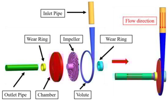
Figure 1.
Three-dimensional model of the USSPAT.

Table 1.
Basic parameters of USSPAT.
3.2. Mesh and Mesh Independence Analysis
The computational domain of the USSPAT in this study is divided into five components: the inlet and outlet sections, volute, impeller, chamber, and wear rings. The entire domain was meshed using structured grids generated in the ANSYS ICEM 2021, as shown in Figure 2a. Accurate simulation of flow characteristics in the near-wall region necessitates a refined treatment of the boundary layer. Consequently, a mesh refinement strategy was implemented on critical surfaces, including the blade surfaces, leading edges, and trailing edges, to improve the resolution of the flow phenomena near the wall. To ensure the accurate capture of small-scale structures within the blade boundary layer, more than 15 nodes were placed within the first boundary layer mesh. The resulting Y+ distribution on the blade surfaces is presented in Figure 2b. The average Y+ values for the impeller and volute regions are presented in Table 2, with the maximum Y+ value on the blade surface being less than 10, which meets the requirements for numerical simulation.
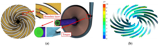
Figure 2.
(a) Computational mesh of the fluid domain; (b) Blade Surface Y+ Distribution.
Table 2.
Basic parameters of USSPAT. Mean values of y+ on wall surface.
The mesh density significantly impacts both the prediction accuracy of USSPAT performance and computational time. To ensure simulation precision while improving computational efficiency, a grid independence study was conducted for the USSPAT. Eight distinct mesh schemes with varying cell counts were generated for numerical simulation. Figure 3 presents the computational results under different mesh densities, demonstrating that the output power of the USSPAT increases continuously with mesh refinement. When the cell count reaches 7.94 million, further mesh densification yields negligible changes in output power. Accordingly, the mesh configuration with 7.94 million cells was ultimately adopted for all subsequent computations.
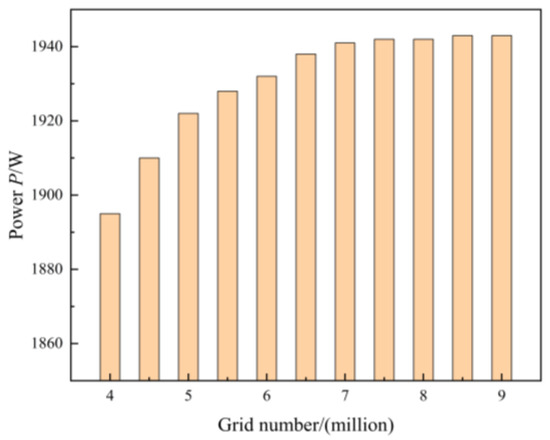
Figure 3.
PAT power output under different grid densities.
3.3. Numerical Settings
The numerical simulations of the USSPAT were conducted using ANSYS Fluent 2021. The working fluid was water at standard temperature and pressure. A pressure inlet boundary condition, consistent with the experimental setup, was applied at the inlet, with the reference pressure set to 0 Pa. A mass flow rate condition was specified for the outlet. The computational domain was divided into a rotating domain for the impeller and stationary domains for all other components. The surfaces of the impeller blades and shrouds were set as rotating walls, while all other solid surfaces were defined as stationary no-slip walls. The schematic diagram illustrating the interfaces of the USSPAT is presented in Figure 4. The simulation was performed in two stages. First, a steady-state simulation was conducted using the SST k-ω turbulence model to obtain a converged initial flow field. This result was then used as the starting point for the unsteady simulation, which employed the DES hybrid RANS/LES model. For the unsteady calculation, the time step was set to 3.333 × 10⁻⁴ s, corresponding to a 3° rotation of the impeller per step. The simulation was run for a total of 10 full revolutions to ensure that the flow field reached a periodically stable state.
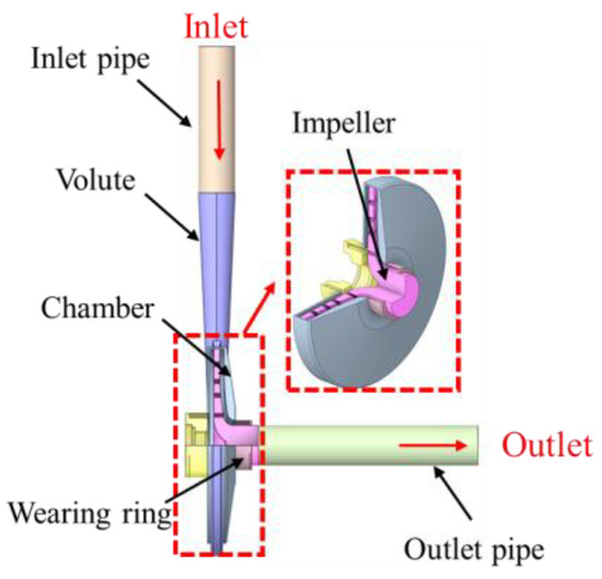
Figure 4.
Schematic diagram of the USSPAT interfaces.
3.4. Experimental Verification
To validate the accuracy of the numerical simulations, an experimental test rig for the PAT was constructed. A three-dimensional model of the test rig is shown in Figure 5, and the experimental test rig for the PAT is presented in Figure 6. The key performance parameters, including the head, power, and efficiency, were calculated from the experimental data using Equations (32), (33), and (34), respectively.
where M is the torque output of the PAT, n is the rotational speed, Pin and Pout are the total pressures at the PAT inlet and outlet, respectively, Q is the flow rate, g is the gravitational acceleration, and H is the head.
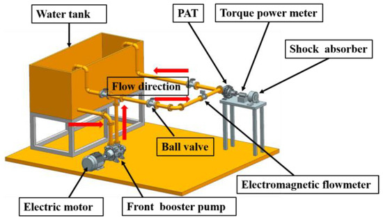
Figure 5.
3D model of the USSPAT test rig.
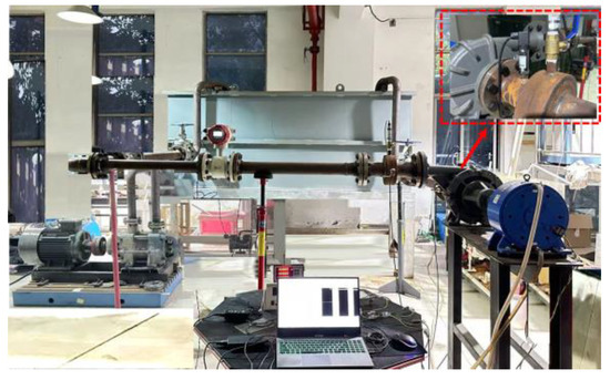
Figure 6.
The experimental test rig for the USSPAT.
In this experiment, the inlet pressure of the PAT was controlled by adjusting the speed of an front booster pump via a frequency converter, and the flow rate was regulated using a valve at the pipeline outlet. The real-time inlet and outlet pressures of the PAT were measured by HM22-2-V2-F1W1 pressure sensors, which have a measurement range of 0–1 MPa. The uncertainty of the sensors is ±0.25% of the full scale, corresponding to an absolute uncertainty of ±2.5 kPa. For the pressure pulsation analysis, the data acquisition system sampled the sensor’s output signal at a frequency of 2000 Hz, and the 16-bit data acquisition card provided a system resolution of approximately 15.2 Pa. an electromagnetic flowmeter measured the flow rate, and a torque meter measured the rotational speed and torque. Subsequently, the acquired data was analyzed and processed by the testing software to obtain the real-time efficiency, head, and output shaft power.
To validate the reliability of the experimental results, an uncertainty analysis was conducted in this study. The total uncertainty comprises random uncertainty, arising from fluctuations in the measured data, and systematic uncertainty, caused by instrumental and system errors.
The formula for calculating the total uncertainty is as follows:
Table 3 presents the detailed uncertainty calculation for the design flow rate condition. The combined uncertainty of the experimental test rig system is ±0.34%, which meets the required precision standards.
Table 3.
Uncertainty calculation results.
The experimental results indicate that the output power of the USSPAT increases with the flow rate. As shown in Figure 7, under the design operating condition, the experimentally measured power and efficiency of the USSPAT were 2.0 kW and 52.28%, respectively, compared to the numerical predictions of 1.94 kW and 51.65%. Overall, the trend observed in the numerical simulation is in good agreement with the experimental data. The relative deviation between the numerical and experimental results for both power and efficiency is less than 5%, which confirms that the simulation method meets the required accuracy standards.
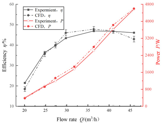
Figure 7.
Comparison of the numerical simulation and experimental results for the USSPAT.
4. Results and Discussions
4.1. Pressure Pulsation Analysis of USSPAT
The characteristic frequency parameters of the USSPAT at the rated speed are as follows, at 1500 rpm, the shaft frequency is f0 = n/60 = 25 Hz, and the BPF is 16 × f0 = 400 Hz. Fast Fourier Transform (FFT) was performed on the dimensionless pressure coefficient CP using MATLAB 2023. As shown in Figure 5, a pressure sensor was installed at the PAT outlet to measure pressure pulsations under different flow conditions. The instantaneous pressure data acquired by the sensor were normalized using CP for dimensional uniformity and comparative analysis. The expression for CP is given as follows:
Figure 8 presents the experimentally measured time-domain plots of pressure pulsations under different flow rates. At the rotational speed of 1500 rpm, the fluctuation amplitude of the CP is on the order of ±5 × 10⁻⁴ at low flow rates, increasing to the order of ±1 × 10⁻³ at high flow rates. The overall variation remains relatively stable across the conditions. At 0.8Qd, the periodicity of the waveform is not pronounced. This is primarily attributed to the significant influence of vortices, secondary flows, and potential backflow in the outlet flow field under low flow rate conditions, which results in a complex frequency spectrum. Conversely, at higher flow rates, particularly at 1.4Qd, the periodicity becomes much more evident, with the peaks exhibiting a quasi-periodic arrangement. At this condition, a clear pulsation phenomenon dominated by a quasi-single frequency emerges, which is likely attributable to the influence of the BPF. However, at 1.6Qd, the flow unsteadiness is enhanced, but a single dominant periodicity is absent. This is mainly because the flow is characterized by the coexistence and interaction of turbulent pulsations and large-scale vortices. The analysis reveals that the pulsation intensity is lowest at the 0.8Qd condition. However, the waveform at this point lacks clear periodicity and exhibits irregular characteristics, which is primarily attributed to the influence of non-periodic, large-scale vortex structures and potential backflow under low flow rate conditions. In contrast, while the overall pulsation intensity at the 1.0Qd condition is higher than that at 0.8Qd, its signal is highly regular and displays significant periodic features. This periodicity is directly linked to the BPF, as confirmed by the frequency-domain analysis. Therefore, although the 0.8Qd condition has the minimum pulsation intensity, the 1.0Qd condition represents the most periodically stable operating point.
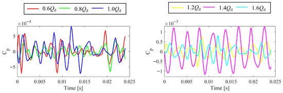
Figure 8.
Time-domain plots of pressure pulsations at the outlet of the PAT under different flow rates.
Figure 9 and Figure 10 present the time-frequency distributions of pressure pulsations at the turbine outlet monitoring point, obtained from the experimental measurements and numerical simulations, respectively. Overall, a strong agreement is observed between the experimental and numerical results regarding the evolution of the spectral characteristics with varying flow rates. At 1.0Qd, the flow field exhibits a high degree of stability and periodicity. Under the 0.8Qd in Figure 9 and Figure 10, the pulsation energy is predominantly concentrated within a narrow and distinct band at the BPF (St = 16), and this energy is uniformly distributed across the time domain. This indicates that under this condition, the pressure pulsations are primarily dominated by the periodic RSI resulting from the impeller’s rotation. Meanwhile, low-frequency instabilities, which are typically induced by flow separation or large-scale vortex structures, are effectively suppressed. At 0.8Qd, a significant region of energy concentration emerges in the low-frequency domain (St < 8). The experimental plot in Figure 9’s 1.0Qd reveals that these high-energy zones are intermittent in the time domain. This intermittency reflects the stochastic nature of real-world turbulence, where broadband turbulent fluctuations cause the energy associated with specific frequency bands to appear as intermittent features in the time-frequency plot. In contrast, the numerical results from the URANS method (Figure 9) exhibit a clean and continuous low-frequency energy band, failing to reproduce this stochastic intermittency. This is because the URANS approach is primarily designed to capture large-scale, deterministic periodic structures while averaging out the finer-scale, chaotic turbulent fluctuations. At 1.2Qd, the intensity of the outlet pressure pulsations reaches its maximum. The energy band at the BPF (St = 16) is not only at its highest intensity but is also significantly broadened. This is primarily caused by the intensified RSI at the high flow rate, coupled with strong turbulence induced by flow separation on the blade suction side. Concurrently, the energy in the low-frequency domain is also amplified. However, it manifests as a continuous, broadband noise signature, which is distinct from the intermittent vortex characteristics observed at low flow rates. This phenomenon is attributed to the interaction of multi-scale turbulent eddies under conditions of high turbulence intensity.
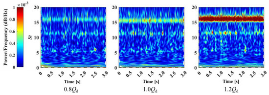
Figure 9.
Time-frequency analysis of the experimental outlet pressure pulsations for the PAT under different flow rates.
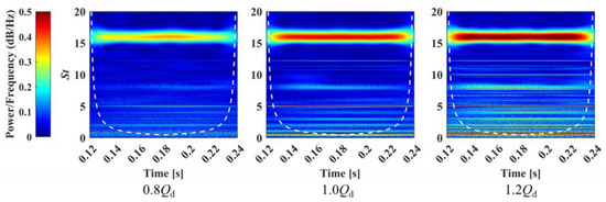
Figure 10.
Time-frequency analysis of the numerical outlet pressure pulsations for the PAT under different flow rates.
Notably, a significant discrepancy exists in the secondary frequency components between the experimental and numerical results. The numerical simulations clearly show a distinct energy band at St = 8, which is primarily attributed to the impeller’s alternating long and short blade design. This geometric feature creates an asymmetric flow field in adjacent passages, thus generating a characteristic frequency at St = 8 (0.5 BPF). In contrast, the experimental data consistently exhibits a dominant secondary frequency at St ≈ 12. This is mainly attributed to the excitation of a natural mode of the experimental test system, likely originating from acoustic resonance within the piping system. When the flow pulsations couple with this mode, its energy is significantly amplified.
4.2. Internal Entropy Production Analysis of USSPAT
Local entropy generation is mainly divided into three types: direct dissipation entropy generation (), caused by viscous dissipation; turbulent dissipation entropy generation (), caused by turbulent dissipation; and wall entropy generation (ΔSPRO,W), caused by boundary layer effects. To better understand the types of entropy generation in the PAT under different flow rates, Figure 11 and Figure 12, respectively, show the values and proportion distribution of each entropy generation type under different operating conditions. It can be seen from the figures that the values of turbulent dissipation entropy generation and wall entropy generation both increase as the flow rate increases, which indicates that the internal energy loss within the PAT increases accordingly. By observing the entropy generation proportion curves, it can be found that as the flow rate increases, the proportions of turbulent dissipation entropy generation and direct dissipation entropy generation gradually decrease, while the proportion of wall dissipation entropy generation gradually increases. The proportion of direct dissipation entropy generation is less than 3%, reaching its value of 2.5% at 0.6Qd. The proportions of turbulent dissipation entropy generation and wall dissipation entropy generation are very large under different operating conditions. Among them, the proportion of turbulent dissipation entropy generation exceeds 50% under all conditions, reaching 56.2% at 0.6Qd. The proportion of wall dissipation entropy generation is at its minimum at 0.6Qd, with a value of 41.3%. Therefore, turbulent dissipation entropy generation and wall dissipation entropy generation can be regarded as the main sources of energy loss during the operation of the USSPAT, and the viscous dissipation entropy generation can be considered negligible.
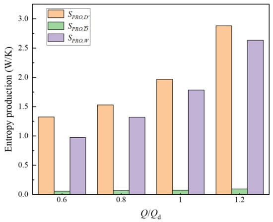
Figure 11.
Different types of entropy production in the USSPAT.
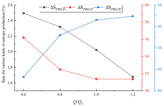
Figure 12.
Entropy generation proportion distribution in the USSPAT under different flow rates.
Figure 13 illustrates the distribution of entropy generation proportions among the different flow passage components of the PAT under various flow rates. Among these, the impeller, volute, and chamber consistently account for the largest shares of the total entropy generation across all flow rates, identifying them as the critical regions of energy loss. As the flow rate increases, the proportion of entropy generation in the impeller first decreases and then increases, reaching a minimum at 0.8Qd. This is primarily attributed to the mismatch between the inlet flow velocity and the blade inlet angle that occurs under low flow rate conditions. In contrast, the entropy generation proportion of the volute exhibits the opposite trend, initially increasing before decreasing. The energy loss proportions for the outlet section and the wear ring area follow a nearly identical trend, with both remaining at a relatively low level.
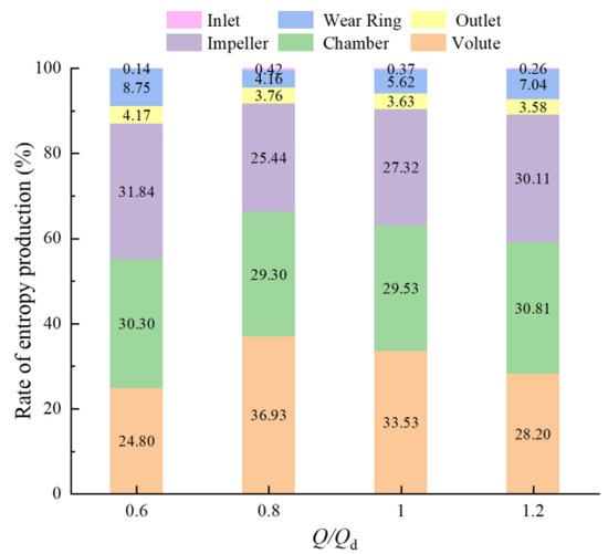
Figure 13.
Entropy generation proportion distribution in the PAT under different flow rates.
As indicated by the preceding analysis, the impeller is a critical region of energy loss in the PAT, and its internal losses are significantly influenced by the flow rate. Figure 14 presents the entropy generation rate distribution on the impeller mid-span at various flow rates. The figure reveals that regions of high entropy generation rate are primarily concentrated at the impeller inlet, outlet, and within the flow passage near the volute tongue. Furthermore, these high-entropy regions expand as the flow rate increases. A high entropy generation rate is observed at the trailing edge of the long blades; this is likely attributed to flow separation in the impeller outlet region, which is induced by the increased flow rate and results in more disordered flow. The entropy generation at the blade trailing edges and the impeller outlet increases significantly with the flow rate, indicating that the increased flow rate leads to a more disordered flow field in the impeller outlet region. At 0.6Qd, the outlet region of the long blades shows almost no areas of high entropy generation. The high-entropy regions within the impeller mostly coincide with areas of vortex formation, indicating that vortices are a significant factor in causing energy loss.
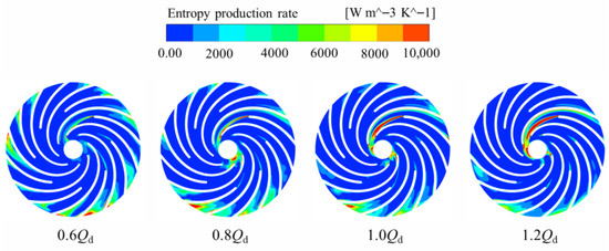
Figure 14.
Local entropy generation distribution on the impeller mid-span at various flow rates.
As established in the previous analysis, wall entropy generation is a significant source of energy loss during the operation of the PAT. Figure 15 illustrates the wall entropy generation distribution on the impeller surfaces at various flow rates. Regions of high entropy generation are primarily located in the flow passages near the volute tongue, at the trailing edges of the long and short blades, and in the impeller inlet region. Furthermore, as the flow rate increases, both the intensity and extent of entropy generation in the passages near the volute tongue expand, which is attributed to flow separation induced by the high-velocity fluid interactions occurring in this region. Under low flow rate conditions, the high-entropy regions are highly concentrated on the suction side near the blade leading edge. This is because the low flow rate causes the fluid to impinge on the blades at a large positive angle of attack, thereby inducing large-scale flow separation. The intense velocity gradients and turbulent fluctuations within the separation bubble and its reattachment zone constitute the primary cause of energy loss in this region. Under high flow rate conditions, the high-entropy regions shift entirely to the blade outlet region and are predominantly distributed on the pressure side and the adjacent shroud wall. This occurs because at high flow rates, the fluid enters the blade passage at a negative angle of attack, and concurrently, a typical jet-wake structure is formed at the blade passage outlet under the combined effect of centrifugal and Coriolis forces. The intense shearing effects between the high-velocity jet region and the wall surfaces, as well as at the interface between the jet and the wake, constitute the main source of energy loss under this condition.
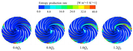
Figure 15.
Wall entropy generation distribution on the impeller at various flow rates.
4.3. Modal Analysis of the Internal Flow in the USSPAT
To further analyze the coherent structures and unsteady flow within the PAT, the DMD method was applied to the snapshot data of the internal flow fields in the impeller and volute. Given the periodic nature of the flow field in the PAT, the analysis was based on 360 snapshots of the velocity distribution data, captured over one full impeller revolution at the 1.0Qd operating condition.
A modal decomposition was performed on the impeller velocity field. Figure 16a shows the resulting eigenvalue distribution from the DMD analysis. It is observed that the eigenvalues are located predominantly on or near the unit circle, with only a few located inside the circle. This indicates that the flow field within the impeller under this condition is primarily composed of periodic or stable modes. Since the eigenvalues appear in complex conjugate pairs, they are symmetric about lg (λ), and each conjugate pair represents a single oscillatory mode. Eigenvalues situated on the unit circle correspond to flow structures that are periodically stable, while those inside the unit circle represent weakly decaying. Therefore, the modes extracted from the DMD of the impeller flow field at 1.0Qd are predominantly stable. Figure 16b shows the decay rate distribution of the impeller velocity field modes. The decay rates of the first several modes are predominantly greater than zero, indicating that these modes do not exhibit temporal decay. Figure 17 presents the modal energy distribution of the impeller, where modal energy serves to evaluate the relative contribution of each mode to the flow field dynamics. The modes with the highest energy are all concentrated in the low-frequency range. The first four modes correspond to frequencies of 25, 50, 75, and 100 Hz, respectively. It can be observed that the frequencies of these first four dominant modes are all integer multiples of the shaft frequency.
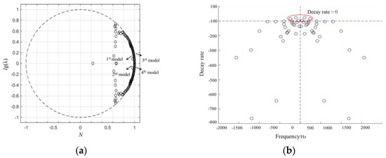
Figure 16.
(a) Impeller eigenvalue distribution; (b) Impeller decay rate distribution.
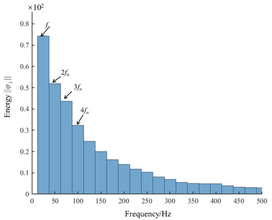
Figure 17.
Distribution of energy in the impeller velocity field.
Figure 18 displays the averaged flow field of the impeller alongside the spatial structures of the first five dominant DMD modes. Among the modes of the PAT velocity field, mode 1 corresponds to the shaft frequency, and its spatial structure closely resembles the time-averaged flow field. As the most energetic mode, it represents the primary periodic fluctuation superimposed on the mean flow. Its coherent structures are primarily concentrated at the impeller inlet, characterized by a distinct high-velocity region near the pressure side of the blades, exhibiting a circumferential symmetry related to the blade count. This clearly reveals the formation of high-velocity fluid pockets at the impeller inlet, which is a direct consequence of the RSI between the volute and the impeller. Therefore, mode 1 is identified as the fundamental RSI mode. Mode 2, corresponding to a frequency of 50 Hz (2f0), features coherent structures distributed throughout the flow passage, with a notable presence at the impeller inlet, suggesting it is associated with unsteady phenomena such as flow recirculation in this region. Modes 3 and 4, corresponding to 3f0 and 4 f0, respectively, represent higher-order harmonics of the fundamental RSI mode, indicating the influence of the impeller’s rotation on the flow field through RSI. The coherent structures of modes 3 and 4 are mainly distributed near the impeller inlet, and their velocity distributions are similar, showing an alternating pattern of maxima and minima. As the mode order increases, the circumferential wavenumber of the spatial structures also increases, manifesting as a greater number of alternating positive and negative velocity fluctuation zones around the circumference. This reflects the emergence of smaller-scale flow details under the influence of RSI. The concentration of their energy near the impeller inlet confirms that these higher-frequency pulsations remain closely linked to the RSI. The spatial structure of mode 5 is markedly different from the preceding harmonic modes. Its energy is not uniformly distributed at the impeller inlet but is instead localized at the junction where the main flow passage meets the splitter blades. This is primarily attributed to the shedding of vortex structures originating from flow separation at this junction. Compared to modes 3 and 4, mode 5 consists of a larger number of smaller-scale, less symmetric coherent structures, which reflects the breakup and dissipation of unstable fluid parcels within the impeller passages.
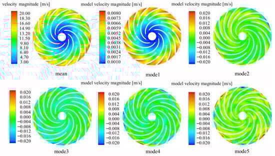
Figure 18.
Average velocity field and distribution of the first five modes in the impeller.
Figure 19 presents the eigenvalue distribution and the decay rate distribution obtained from the DMD of the volute velocity field. Regarding the overall stability of the flow field, Figure 19a reveals that the vast majority of eigenvalues are clustered on or within the unit circle, with no eigenvalues located outside of it. This indicates that the flow field within the volute is dominated by a combination of periodic and decaying modes, and the flow is globally stable. Figure 19b shows the distribution of modal decay rates. It can be observed that the vast majority of modes exhibit negative decay rates, corresponding to stable structures that attenuate over time. In contrast, a few dominant modes are observed with eigenvalues on or very near the unit circle, corresponding to near-zero growth/decay rates. These modes represent the dominant and persistent oscillatory structures within the flow. It is important to clarify that the slightly positive growth rates exhibited by these dominant modes do not indicate a future system instability or “blow-up.” Instead, in the context of the non-linear, saturated system simulated here, this signifies that these modes are actively sustained by a continuous transfer of energy from the mean flow, which balances their natural dissipative decay, thereby maintaining a stable oscillation.
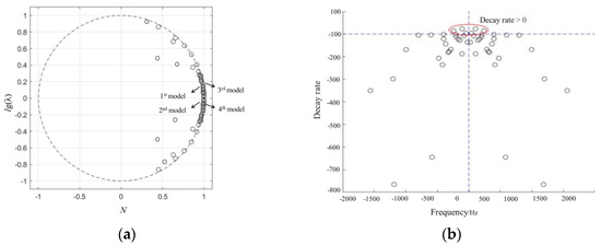
Figure 19.
(a) Volute eigenvalue distribution; (b) Volute decay rate distribution.
Figure 20 presents the averaged flow field on the volute mid-span, along with the first five dominant DMD modes. It can be observed that the spatial structure of mode 1 closely resembles the distribution of the mean flow field, clearly delineating the velocity distribution in the diffuser and spiral sections of the volute. In mode 2, a region of alternating local maxima and minima appears at the interface between the volute and the impeller. Furthermore, due to the disturbance from the volute tongue, the flow structures near the tongue differ in scale from those in other regions. Mode 3 also exhibits 16 alternating structures at the interface. The number of these structures corresponds exactly to the number of impeller blades, indicating that this pattern is a classic manifestation of RSI. Mode 4 likewise displays characteristics of circumferential periodicity. However, in contrast to modes 2 and 3, the alternating structures in mode 4 are smaller in scale and more numerous. This mode represents a higher-order harmonic of the RSI phenomenon. Mode 5 does not exhibit a distinct, regular pattern; instead, it is characterized by prominent velocity gradients located within the spiral section of the volute. Overall, the flow dynamics within the volute are clearly influenced by the impeller’s rotation. The primary source of unsteadiness in the flow field is the RSI between the impeller and the volute, which manifests as the alternating structure of local extrema at the interface. This phenomenon is primarily captured by modes 2 and 3. mode 4 is identified as a higher-order harmonic related to these fundamental RSI modes, while mode 5 also constitutes an important component of the flow’s dynamic characteristics, reflecting the overall complexity of the RSI phenomenon.
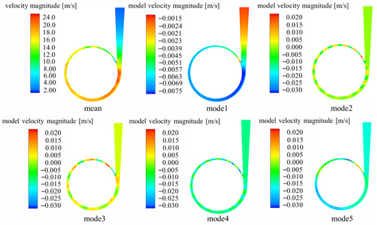
Figure 20.
Average velocity field in the volute casing and distribution of the first five modes.
5. Conclusions
In this study, the internal flow field and energy losses of a USSPAT were investigated using entropy generation theory and the DMD method. The accuracy of the numerical simulations was validated by experimental data, and the following main conclusions were drawn:
- (1)
- Analysis of pressure pulsations reveals that the BPF (St = 16) is the absolute dominant frequency under all operating conditions, with its intensity increasing as the flow rate rises. This indicates that the pressure pulsations are predominantly governed by the periodic rotor-stator interaction resulting from the impeller rotation. The flow is characterized by quasi-periodic vortex bands at low flow rates, which evolves into broadband turbulence at high flow rates. Furthermore, a distinct pulsation characteristic at half the BPF, associated with the long-and-short blade configuration, was identified. This pulsation is attributed to asymmetric flow separation and the subsequent vortex shedding within the impeller passages.
- (2)
- Internal energy losses in the PAT are primarily composed of turbulent and wall dissipation and are mainly localized within the impeller, volute, and side chamber. The entropy generation from these three components accounts for approximately 90% of the total entropy generation in the PAT. Within the impeller, the energy losses are concentrated at the inlet, outlet, and in the passage near the volute tongue. As the flow rate increases, these high-entropy-generation regions expand. Crucially, the high-entropy regions within the impeller largely coincide with areas of vortex formation, indicating that vortices are a key contributor to energy loss.
- (3)
- The DMD results reveal the dominant modes of the internal flow field. Within the impeller, the first four dominant modes are predominantly low-frequency, with their frequencies corresponding to integer multiples of the shaft frequency. This demonstrates that the internal flow is dominated by periodic, RSI-driven modes, with energy concentrated in the low-frequency range. Among them, the first-order mode is characterized as the RSI mode, whereas the third- and fourth-order modes are identified as higher-order harmonics of this RSI mode. The flow dynamics within the volute are, in turn, significantly influenced by the impeller’s rotation. Fundamentally, the primary source of unsteadiness in the flow field is the RSI between the impeller and the volute. This interaction manifests as an alternating structure of extrema at the interface, which is identified as the root cause of both the pressure pulsations and the periodic energy losses.
Author Contributions
W.Z.: review and editing, methodology, data curation. Y.S.: Writing—original draft, formal analysis. B.W.: Software, methodology. Y.W.: supervision, resources. J.Y.: investigation, funding acquisition, methodology. All authors have read and agreed to the published version of the manuscript.
Funding
This work was supported by the Special fund of technological innovation for carbon peak and carbon neutrality in Jiangsu Province (BE2022032-3).
Data Availability Statement
The raw data supporting the conclusions of this article will be made available by the authors on request.
Conflicts of Interest
The authors declare that this research was conducted in the absence of any commercial or financial relationships that could be construed as potential conflicts of interest.
Abbreviations
The following abbreviations are used in this manuscript:
| PAT | Pump as turbine |
| USSPAT | Ultra-low specific speed pump as turbine |
| CFD | Computational fluid dynamics |
| SST | Shear Stress Transport |
| FFT | Fast Fourier transform |
| RANS | Reynolds-averaged Navier–Stokes |
| CWT | Continuous wavelet transform |
| BPF | Blade passing frequency |
| RSI | Rotor-stator interaction |
| PIV | Particle image velocimetry |
| SVD | Singular value decomposition |
References
- Hu, H.S.; Dong, W.H. The Goal of Carbon Peaking, Carbon Emissions, and the Economic Effects of China’s Energy Planning Policy: Analysis Using a CGE Model. Int. J. Environ. Res. Public Health 2023, 20, 165. [Google Scholar] [CrossRef]
- Hanif, I.; Aziz, B.; Chaudhry, I.S. Carbon emissions across the spectrum of renewable and nonrenewable energy use in developing economies of Asia. Renew. Energy 2019, 143, 586–595. [Google Scholar] [CrossRef]
- Scherer, L.; Pfister, S. Global water footprint assessment of hydropower. Renew. Energy 2016, 99, 711–720. [Google Scholar] [CrossRef]
- Nautiyal, H.; Varun; Kumar, A. Reverse running pumps analytical, experimental and computational study: A review. Renew. Sustain. Energy Rev. 2010, 14, 2059–2067. [Google Scholar] [CrossRef]
- Morabito, A.; Hendrick, P. Pump as turbine applied to micro energy storage and smart water grids: A case study. Appl. Energy 2019, 241, 567–579. [Google Scholar] [CrossRef]
- Agarwal, T. Review of pump as turbine (PAT) for micro-hydropower. Int. J. Emerg. Technol. Adv. Eng. 2012, 2, 163–169. [Google Scholar]
- Binama, M.; Su, W.T.; Li, X.B.; Li, F.C.; Shi, X.Z.; An, S. Investigation on pump as turbine (PAT) technical aspects for micro hydropower schemes: A state-of-the-art review. Renew. Sustain. Energy Rev. 2017, 79, 148–179. [Google Scholar] [CrossRef]
- Lin, T.; Zhu, Z.C.; Li, X.J.; Li, J.; Lin, Y.P. Theoretical, experimental, and numerical methods to predict the best efficiency point of centrifugal pump as turbine. Renew. Energy 2021, 168, 31–44. [Google Scholar] [CrossRef]
- Derakhshan, S.; Nourbakhsh, A. Theoretical, numerical and experimental investigation of centrifugal pumps in reverse operation. Exp. Therm. Fluid Sci. 2008, 32, 1620–1627. [Google Scholar] [CrossRef]
- Giosio, D.; Henderson, A.; Walker, J.; Brandner, P.; Sargison, J.; Gautam, P. Design and performance evaluation of a pump-as-turbine micro-hydro test facility with incorporated inlet flow control. Renew. Energy 2015, 78, 1–6. [Google Scholar]
- Sun, X.; Huang, H.; Zhao, Y.; Tong, L.; Lin, H.; Zhang, Y. A Review of Methods for” Pump as Turbine”(PAT) Performance Prediction and Optimal Design. Fluid Dyn. Mater. Process. 2025, 21, 1261–1298. [Google Scholar] [CrossRef]
- Miao, S.; Zhang, H.; Tian, W.; Li, Y. A study on the unsteady flow characteristics and energy conversion in the volute of a pump-as-turbine device. Fluid Dyn. Mater. Process. 2021, 17, 1021–1036. [Google Scholar]
- Binama, M.; Su, W.T.; Cai, W.H.; Li, X.B.; Muhirwa, A.; Li, B.; Bisengimana, E. Blade trailing edge position influencing pump as turbine (PAT) pressure field under part-load conditions. Renew. Energy 2019, 136, 33–47. [Google Scholar] [CrossRef]
- Lin, T.; Zhang, J.R.; Li, J.; Li, X.J.; Zhu, Z.C. Pressure Fluctuation-Vorticity Interaction in the Volute of Centrifugal Pump as Hydraulic Turbines (PATs). Processes 2022, 10, 2241. [Google Scholar] [CrossRef]
- Xiang, R.; Wang, T.; Fang, Y.J.; Yu, H.; Zhou, M.; Zhang, X. Effect of blade curve shape on the hydraulic performance and pressure pulsation of a pump as turbine. Phys. Fluids 2022, 34, 085130. [Google Scholar] [CrossRef]
- Chai, B.D.; Yang, J.H.; Wang, X.H.; Jiang, B.X. Pressure Fluctuation Characteristics Analysis of Centrifugal Pump as Turbine in Its Start-Up Process. Actuators 2022, 11, 132. [Google Scholar] [CrossRef]
- Lin, T.; Li, J.; Xie, B.F.; Zhang, J.R.; Zhu, Z.C.; Yang, H.; Wen, X.M. Vortex-Pressure Fluctuation Interaction in the Outlet Duct of Centrifugal Pump as Turbines (PATs). Sustainability 2022, 14, 15250. [Google Scholar] [CrossRef]
- Ran, H.J.; Luo, X.W.; Zhu, L.; Zhang, Y.; Wang, X.; Xu, H.Y. Experimental study of the pressure fluctuations in a pump turbine at large partial flow conditions. Chin. J. Mech. Eng. 2012, 25, 1205–1209. [Google Scholar] [CrossRef]
- Shen, S.M.; Qian, Z.D.; Ji, B. Numerical Analysis of Mechanical Energy Dissipation for an Axial-Flow Pump Based on Entropy Generation Theory. Energies 2019, 12, 4162. [Google Scholar] [CrossRef]
- Gong, R.Z.; Qi, N.M.; Wang, H.J.; Chen, A.L.; Qin, D.Q. Entropy Production Analysis for S-Characteristics of a Pump Turbine. J. Appl. Fluid Mech. 2017, 10, 1657–1668. [Google Scholar] [CrossRef]
- Liu, M.; Tan, L.; Cao, S.L. Theoretical model of energy performance prediction and BEP determination for centrifugal pump as turbine. Energy 2019, 172, 712–732. [Google Scholar] [CrossRef]
- Nishi, Y.; Suzuo, R.; Sukemori, D.; Inagaki, T. Loss analysis of gravitation vortex type water turbine and influence of flow rate on the turbine’s performance. Renew. Energy 2020, 155, 1103–1117. [Google Scholar] [CrossRef]
- Ghorani, M.M.; Haghighi, M.H.S.; Maleki, A.; Riasi, A. A numerical study on mechanisms of energy dissipation in a pump as turbine (PAT) using entropy generation theory. Renew. Energy 2020, 162, 1036–1053. [Google Scholar] [CrossRef]
- Zhu, Z.; Gu, Q.; Chen, H.; Ma, Z.; Cao, B. Investigation and optimization into flow dynamics for an axial flow pump as turbine (PAT) with ultra-low water head. Energy Convers. Manag. 2024, 314, 118684. [Google Scholar] [CrossRef]
- Wang, C.; Zhang, Y.X.; Hou, H.C.; Zhang, J.Y.; Xu, C. Entropy production diagnostic analysis of energy consumption for cavitation flow in a two-stage LNG cryogenic submerged pump. Int. J. Heat Mass Transf. 2019, 129, 342–356. [Google Scholar] [CrossRef]
- Shu, Z.K.; Shi, G.T.; Dan, Y.; Wang, B.X.; Tan, X. Enstrophy dissipation of the tip leakage vortex in a multiphase pump. Phys. Fluids 2022, 34, 033310. [Google Scholar] [CrossRef]
- Zhang, Y.; Jiang, W.; Qi, S.W.; Xu, L.; Wang, Y.C.; Chen, D.Y. Clocking effect on the internal flow field and pressure fluctuation of PAT based on entropy production theory. J. Energy Storage 2023, 69, 107932. [Google Scholar] [CrossRef]
- Xin, T.; Wei, J.; Li, Q.Y.; Hou, G.Y.; Ning, Z.; Wang, Y.C.; Chen, D.Y. Analysis of hydraulic loss of the centrifugal pump as turbine based on internal flow feature and entropy generation theory. Sustain. Energy Technol. Assess. 2022, 52, 102070. [Google Scholar] [CrossRef]
- Li, D.Y.; Wang, H.J.; Qin, Y.L.; Han, L.; Wei, X.Z.; Qin, D.Q. Entropy production analysis of hysteresis characteristic of a pump-turbine model. Energy Convers. Manag. 2017, 149, 175–191. [Google Scholar] [CrossRef]
- Guang, W.L.; Liu, Q.; Jin, F.Y.; Tao, R.; Xiao, R.F. Analysis of clearance flow of a fuel pump based on dynamical mode decomposition. J. Hydrodyn. 2024, 36, 781–795. [Google Scholar] [CrossRef]
- Li, Y.B.; He, C.H.; Li, J.Z. Study on Flow Characteristics in Volute of Centrifugal Pump Based on Dynamic Mode Decomposition. Math. Probl. Eng. 2019, 2019, 2567659. [Google Scholar] [CrossRef]
- Schmid, P.J. Dynamic mode decomposition of numerical and experimental data. J. Fluid Mech. 2010, 656, 5–28. [Google Scholar] [CrossRef]
- Long, Y.; Xu, Y.; Guo, X.A.; Zhang, M.Y. Analysis of internal flow excitation characteristics of reactor coolant pump based on DMD. Ann. Nucl. Energy 2025, 211, 111011. [Google Scholar]
- Han, Y.D.; Tan, L. Dynamic mode decomposition and reconstruction of tip leakage vortex in a mixed flow pump as turbine at pump mode. Renew. Energy 2020, 155, 725–734. [Google Scholar] [CrossRef]
- Miao, S.; Liu, L.; Wang, X.; Yang, J. Unsteady flow analysis in a pump as turbine impeller based on proper orthogonal decomposition and dynamic mode decomposition methods. Phys. Fluids 2024, 36, 115186. [Google Scholar] [CrossRef]
- Li, P.X.; Dong, W.; Jiang, H.Q.; Zhang, H.C. Analysis of axial force and pressure pulsation of centrifugal pump as turbine impeller based on dynamic mode decomposition. Phys. Fluids 2024, 36, 035141. [Google Scholar] [CrossRef]
- Wang, J.B.; Zeng, L.C.; Yu, S.; He, Y.T.; Tang, J.H. Experimental and numerical investigations of tube inserted with novel perforated rectangular V-shape vortex generators. Appl. Therm. Eng. 2024, 249, 123451. [Google Scholar] [CrossRef]
- Kock, F.; Herwig, H. Local entropy production in turbulent shear flows: A high-Reynolds number model with wall functions. Int. J. Heat Mass Transf. 2004, 47, 2205–2215. [Google Scholar] [CrossRef]


Disclaimer/Publisher’s Note: The statements, opinions and data contained in all publications are solely those of the individual author(s) and contributor(s) and not of MDPI and/or the editor(s). MDPI and/or the editor(s) disclaim responsibility for any injury to people or property resulting from any ideas, methods, instructions or products referred to in the content. |
© 2025 by the authors. Licensee MDPI, Basel, Switzerland. This article is an open access article distributed under the terms and conditions of the Creative Commons Attribution (CC BY) license (https://creativecommons.org/licenses/by/4.0/).