Abstract
This paper revisits the theoretical framework of computing the stabilization value of groundwater in a dynamic context. Specifically, we argue that what the existing studies have measured as the augmentation value contains a different type of value, the dynamic reallocation value (DRV), which should be evaluated as an important part of the dynamic stabilization value. We examine the existence of DRV and its underlying behavioural mechanism using a simple two-stage model and then generalise the specification to a dynamic model with an arbitrary number of stages. We find that behind the positive values of DRV, users amplify their reactions against surface water fluctuations and still realize a higher total expected benefit than in the case without uncertainty. Ignoring the existence of DRV may impair the value of groundwater as an essential instrument for climate adaptation.
1. Introduction
Over the past few decades, a considerable number of studies have attempted to quantify the economic value of groundwater in various locations and explored improved groundwater management (e.g., [1,2,3,4,5,6,7,8,9,10,11,12,13,14]). Most of these attempts are grounded in the theoretical frameworks traced back to Tzur’s seminal papers on the buffering role of groundwater [1,2,5,15]. The basic construction is as follows: the total economic value (TEV) of groundwater can be divided into the augmentation value (AV) and the stabilization value (SV). The AV is the value of being augmented by an increase in the average water intake through the exploitation of groundwater resources in addition to surface water. The SV is the value of mitigating the impact of surface water fluctuation by adjusting groundwater intake.
The present paper revisits this framework in a dynamic context. Specifically, it argues that what existing studies have measured as the AV contains a different type of value generated by users’ dynamic optimizing behaviours, not by the augmentation of the average intake. We call this value the dynamic reallocation value (DRV). We thereby propose a new composition: the TEV is divided into the (pure) augmentation value (AV) and the dynamic stabilization value (DSV), which is the sum of the static stabilization value (SSV) and DRV. Furthermore, using simple analytical models, we uncover the underlying behavioural mechanism that generates the SSV and DRV. We also examine, through numerical illustrations, how each component of the TEV responds to different environment, and how these responses differ under suboptimal environments with multiple users.
The major findings are as follows: First, the stabilization value in dynamic environments is generated from two types of behaviour. One is to mitigate the impact of surface water fluctuation on the current benefit by offsetting it by groundwater intake. The other is to amplify the offsetting behaviours to reallocate the intake intertemporally and save pumping costs over periods. The former generates the SSV and the latter generates the DRV. Second, by leveraging the DRV, even risk-averse users can achieve greater benefits under uncertain conditions compared to environments without surface water fluctuations. Third, the economic benefits of the DRV are greater in areas requiring a longer planning horizon and areas facing a higher pumping cost elasticity to changes in groundwater stock. Fourth, in contrast with previous literature, overexploitation reduces the benefits from stabilization even if physical constraints on extraction capacities do not exist. These findings justify the practical importance of distinguishing the DRV from other components in the economic valuation of groundwater.
2. Theoretical Background and Related Literature
2.1. Theoretical Background of the Stabilization Value
The basic idea of Tsur’s framework is the following. To compute the economic value of groundwater, we first use the difference between the expected net economic benefit of using surface water and groundwater conjunctively and that of using only surface water, taking the latter as a baseline. Specifically, we can calculate the TEV as follows:
where is a strictly concave benefit function, the benefit-maximizing total water use, a unit extraction cost that depends on the groundwater stock, , and is uncertain surface water supply whose known mean is . We assume that is strictly decreasing, that is, the smaller the stock is, the higher the unit cost is. For simplicity, we further assume that the user can utilize surface water for free; therefore, the remaining represents the amount of groundwater used.
The difference obtained in (1), however, contains both the AV and SV. To extract pure SV, Tsur [2] uses the TEV in the case without uncertainty in as another baseline. That is,
where is the benefit-maximizing total water use in the case without uncertainty and is the groundwater stock. The SV is then given by the following:
In this simplified static problem, if the groundwater stocks are equal, that is, and so are the unit costs, then the benefit-maximizing amounts of water use are also the same, , and so are the expected pumping costs. Figure 1 illustrates this. The user maximizes its net economic benefit, by controlling its water use, . To simplify the figure, we assume surface water takes between () and , with a probability of for each and with the mean value . If we assume out the possibility of exhausting the entire stock, we know from the first-order condition, , that, irrespective of the surface water realization, the benefit-maximizing water use, , is determined by point , where the marginal benefit is equal to the marginal cost, . Then, the groundwater intake, , is given by the difference , which means for , for , and for . The pumping cost is thus shown by the area for and for . Therefore, the expected pumping cost in the uncertain case is given by the area , which is equal to the pumping cost in the certain case.
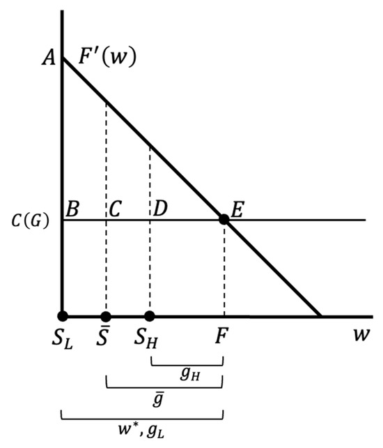
Figure 1.
User’s intake decisions and corresponding benefit and cost. The line segment that is declining to the right is the marginal benefit curve, . The horizontal line represents the marginal cost, .
Since the amount of water use is the same, the expected benefits are also the same between the cases with and without uncertainty, that is, . Also, since the expected pumping costs are the same, we have . As a result, both expected benefits and costs are perfectly offset between the two cases, and only the difference, , is left in Equation (3). This gives a simplified specification of the SV:
As we can see in the figure, the user pumps up the amount that can offset the surface water fluctuation completely and stabilize the benefit, . This is why the SV can eventually be expressed as a risk premium that the user is willing to pay to stabilize the surface water flow at the mean [5].
Using (4), the AV can be computed as the remainder:
which is equal to in Equation (2).
2.2. Related Literature
Various studies, including recent ones [16,17,18,19,20,21,22,23], have referred to Tsur’s argument on the stabilizing function of groundwater, and many empirical studies have adopted the above approach to evaluate the economic value of groundwater in actual water environments. In particular, to compute the SV, most studies have used either the specification of Equation (3) or its simplified version of (4). For example, Tsur [1] applied the former to the northern Negev, Israel, and found that the SV can exceed the groundwater benefit attributed to the increase in water supply. Tsur [3] also applied (3) to the Sari Joaquin Valley in California, United States, and showed that the SV accounts for 47% of the TEV. Similarly, Ranganathan and Palanisami [4] applied (3) to the Srivilliputhur Big Tank in Tamilnadu, India, and found that the SV accounts for 15.7% of the TEV. Palanisami et al. [6] studied the same area using (3) but with a quadratic production function-based empirical estimation of the crop water response and found that the SV accounts for about 19% of the TEV. Kakumanu and Bauer [7] used (3) for Andhra Pradesh, India, and indicated that the TEV and SV are increasing with the decrease in electricity prices and surface water availability. Nanthakumaran and Palanisami [8] also applied (3) to twelve tanks in the Sivagangai and Madurai districts of Tamil Nadu, India, and found that the SV accounts for about 15% of the TEV. Palanisami et al. [9] also studied the same area but examined different scenarios and showed that the share of the SV in the TEV can vary between 7.4% and 23.5%.
On the other hand, Gemma and Tsur [5] applied the specification of Equation (4) to the Coimbatore Water District in Tamil Nadu, India, and showed that the SV accounts for more than 25% of the TEV. Kovacs et al. [10] incorporated the SV calculated by (4) into their spatial dynamic model to examine the optimal groundwater management in the Mississippi River Valley Alluvial Aquifer in the Arkansas Delta, United States. Kovacs and West [11] studied the same area but to examine tradeoffs among the value of ecosystem services and economic returns, and estimated the SV as USD 0.72 and 13.82 per acre-foot. MacEwan et al. [12] implemented the approach of (4) for the case of the Central Valley in California, United States, and found that the SV in three regions in the area has a present value of USD 275 million (USD 2016). Msangi & Hejazi [13] also incorporated (4) in their dynamic model and showed that suboptimal behaviours diminish the AV but keep the SV unaffected when the extraction capacities are not physically limited to the amount that cannot cover the variations in surface water.
However, the transformation from (3) to (4) is not applicable to dynamic cases in general. In a dynamic context, the groundwater stocks in each period are affected by the past intake sequence and so are the expected pumping costs. Therefore, the expected benefits and costs cannot be canceled out between the cases with and without uncertainty. Tsur and Graham-Tomasi [2] were aware of this point. Hence, in their attempt to extend Tsur’s framework to a dynamic environment, they avoided using a simple analogy of the risk premium in (4), but they did not explicitly explore what exists in the gap between (3) and (4). Zhang and Sato [14] also avoided (4) and used a different metric of the SV, but they also did not examine the gap. Other studies, including Gemma and Tsur [5], Kovacs et al. [10], Kovacs and West [11], MacEwan et al. [12], and Msangi and Hejazi [13], have simply applied the specification of (4) to dynamic environments to compute the SV.
The present paper argues that the SV in dynamic environments should be evaluated by the difference between the and , as Equation (3) indicates. But, different from the above existing studies using (3), we argue that this value can be decomposed into two types of value, the SSV and DRV, the latter of which has been measured as part of the AV without realizing it by the above studies using (4), even though the DRV is generated by users’ dynamic optimizing behaviours, not by the augmentation of the average intake. We call the sum of the SSV and DRV the dynamic stabilization value (DSV) to differentiate it from the SSV. Thus, the total economic value of groundwater is eventually composed of three components:
3. Model Formulation
We consider general models with users and denote the user set by . This enables us to examine both optimal and suboptimal multiple-user environments. The former type of solution is described by a single-decision-maker model, where the social planner distributes groundwater intake to each user to maximize the intertemporal sum of the aggregate net economic benefits of all users (henceforth, single-decision-maker regime). The other type of solution is described by a multiple-user model in which each user plays a noncooperative dynamic game in choosing the amount of groundwater intake with the aim of maximizing its own intertemporal sum of net economic benefits (henceforth, multiple-user regime). The former regime can be utilized as a reference to evaluate how the latter deviates from the socially optimal solution. Obviously, replacing provides a simpler scenario for a single user.
The water environment is governed by a stochastic dynamic process determined by two state variables: , groundwater stock at the end of the previous period, and , surface water flow, both available to users at the beginning of period , where and represent sets of possible amounts of the groundwater stock and surface water flow, respectively. The transition equation for the groundwater stock is as follows:
where is the groundwater intake by user in period , and denotes the groundwater recharge. Groundwater dynamics can be governed by a variety of interconnected hydrological processes driven by various climatic, topographic, and hydrogeological factors [24]. However, for analytical simplicity, we do not touch on such complexities and use a fixed value, , throughout all periods. However, such simplifications do not invalidate our argument on the DRV in the following.
Surface water flow, , is given as follows:
where is the average flow amount that is expected in period in normal years and denotes the fluctuation from the average. For the analytic approach in the following section, we assume that is a stationary, temporally independent random variable of a known distribution with a zero mean and variance of . This is a specification that has been used in most conjunctive management literature. For example, the classic work of Burt [25] used independent, identically distributed gamma variates for the stream flows; Tsur himself used an i.i.d. sequence for the surface water fluctuation [2]; Knapp and Olson [26] also used an i.i.d. random variable; and Joodavi et al. [27] used independent and identical Gaussian noise for the effective rainfall. We will discuss the implications of this stationarity and independency assumption and the possibilities of other cases in a later section.
Users make decisions on groundwater intake after observing the realization of surface water flow in each period. This is a typical information scenario of the literature on conjunctive management and corresponds to the ex post case of Tsur and Graham-Tomasi [2]. Let denote the amount of surface water utilized by user , where is ’s share and . For simplicity, we assume that users can use surface water within this range at no additional cost. Let be the total amount of water used by user ; thus, .
represents the instantaneous benefit of user , which is assumed to be quadratic for acquiring analytical solutions:
where and are positive constants. This represents diminishing returns to production, which is the standard economic specification representing the law of diminishing marginal productivity and also accords with most production practices as reported in much of the groundwater literature. For example, in classical groundwater studies, Gisser and Sánchez [28] described net farm income as a quadratic function of irrigation water; Provencher and Burt [29] used a strictly concave function for firms’ periodic benefit; Gardner et al. [30] applied a quadratic benefit function to describe users’ strategic behaviours in groundwater exploitation. In recent studies, Msangi and Hejazi [13] used a quadratic and Quintana-Ashwell and Gholson [17] used a concave benefit function to describe irrigation behaviours.
We introduce user heterogeneity by differentiating s. Although we do not differentiate to obtain analytical solutions for the dynamic game, this differentiation allows us to cover a broad range of heterogeneity in terms of production scale and technology.
Let denote ’s unit pumping cost, which depends on the groundwater stock:
where and are positive constants. Therefore, the cost is inversely proportional to the total inventory. This is consistent with the assumptions of most groundwater studies, such as Gisser and Sánchez [28].
The instantaneous net benefit is given by the following:
The period set is denoted by , and let denote the discounted intertemporal sum of user ’s expected net benefits:
where is the set of admissible actions and is a discount factor. Symbols with the subscript indicate that they are a variable or set for the users excluding . The social planner of the single-decision-maker regime maximizes the discounted intertemporal sum of the aggregate expected net benefits, :
subject to Equations (7) and (8), and the initial stock level, .
In the multiple-user regime, user maximizes the discounted intertemporal sum of the expected net benefits (11) subject to (8), the initial stock level , and the transition equations of the groundwater stock:
Let denote the set of admissible strategies. We can then describe the dynamic process of the multiple-user regime as an -user -stage discrete-time stochastic dynamic noncooperative game defined by .
The summaries of all notations used in the model are listed in Table 1.

Table 1.
List of major notations.
4. Two-Stage Model
We start by demonstrating the existence of a positive DRV by using a simple two-stage model and examine the underlying economic mechanisms.
4.1. Existence of the TEV
By solving backwards from the second stage, we obtain unique solutions for each regime and for cases with and without uncertainty (see SI1 in the Supporting Information for the derivations).
We follow the specification of Equation (3) for the definition of the DSV, that is,
We also follow the specification of Equation (4) for the definition of the SSV, that is,
Accordingly, the SSV represents the pure economic benefit of stabilizing the surface water flow at the mean value [5].
The DRV is given by the residual of subtracting the SSV from the DSV:
We can easily show from the solutions of the two-stage model the following:
Proposition 1.
The dynamic reallocation value (DRV) is positive in both single-decision-maker regimes and multiple-user regimes.
For the full proof, see SI2 in the Supporting Information. The existence of a positive DRV indicates that the transformation from Equations (3) into (4), which has been used repeatedly in the literature, is simply incorrect in dynamic environments.
4.2. User Responses to Surface Water Fluctuation
From the solutions shown in SI1 in the Supporting Information, we can demonstrate how groundwater intake reacts to surface water fluctuation.
Proposition 2.
When the surface water in the first period,, deviates from its mean value by , the aggregate groundwater intake responds to it in the opposite direction by more than in both single-decision-maker regimes and multiple-user regimes. That is,
This is significantly different from the stabilizing behaviour implied by the previous studies using the specification of (4). In these studies, the groundwater intakes respond to the surface water fluctuation on a one-to-one basis to ensure that the former movements perfectly offset the latter variations. However, Proposition 2 suggests that the users do more than just offset the fluctuations but respond to them with greater magnitudes. In other words, the users amplify their reactions against the surface water fluctuation. We also know from Equation (18) that , indicating that the magnitude of the amplification is smaller in a multiple-user regime than a single-decision-maker regime.
From Equation (14), we can derive the following:
The specification of (4) indicates that surface water fluctuations have no effect on the total water use because they are absorbed perfectly by the offsetting movements of the groundwater intake; however, (19) reveals that they do have an effect. When surface water increases, the total water declines and, as surface water decreases, the total water increases.
This destabilizes the total water use and thereby decreases the expected benefit of risk-averse agents in the first period. However, such loss is more than covered in the second period.
Proposition 3.
The aggregate expected net benefit in the first period in the case with uncertainty is less than that in the case without uncertainty. However, the intertemporal sum of the aggregate expected net benefit in the case with uncertainty is greater than that in the case without uncertainty.
For the full proof, see SI3 in the Supporting Information.
4.3. Behavioural Mechanisms of the SSV and DRV
To examine why users respond to surface water fluctuations with greater magnitudes and why such behaviours generate a higher total benefit, we utilize a graphical illustration by simplifying the model in four respects: first, we consider a single-user case, ; second, surface water takes between two values, ( for simplicity) and , with a probability of for each and the mean ; third, there is no recharge (); and fourth, the discount factor . These simplifications are only for the graphical illustration, and the argument below holds for the more general specifications discussed thus far.
In the first stage, after observing surface water, , the user faces the following problem:
where is the solution in the second stage when the first-stage intake was and observing . The first-order condition then provides the benefit-maximizing intake :
The optimal intake is therefore ensured when the marginal benefit is equal to the sum of the unit cost of the first period (the first term on the right side) and the marginal user cost (the second term). The latter is the future pumping cost that would have been saved by decreasing a marginal unit of intake in the first period.
We examine the underlying behavioural mechanism in two steps. First, we introduce a policy in which the user absorbs surface water fluctuation perfectly in the first period and keeps the total water use constant (at the mean value). This is not the optimal behaviour but provides a very good case for understanding the behavioural mechanism of dynamic reallocation. We call this Policy E (where E represents exact stabilization) and denote it by . Next, we introduce the optimal policy described in Proposition 2. In this policy, the user amplifies its reaction against surface water fluctuation but can achieve a full dynamic reallocation value. We call this Policy R (where R represents reallocation) and denote it by . In addition, we call a reference policy that the user would take when there is no uncertainty Policy C (where C represents certainty) and denote it by . In the following figures, we describe the user’s intake decisions and the corresponding benefits and costs after observing (a) and (b) during the first period.
4.3.1. Policy E
Figure 2 shows a comparison of Policies E and C. In Policy C, the total water use in the first period is determined at the intersection of the marginal benefit curve, , and the sum of the unit cost and marginal user cost, . Policy E also maintains this amount by changing the groundwater intake, , to offset the surface water fluctuation in an exact manner. The expected net benefits evaluated in period 0 are the same for both policies. This is exactly the same situation as captured by the simplification of (4).
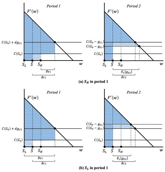
Figure 2.
User’s intake decisions and corresponding net benefits for Policies E and C. The line segment that is declining to the right is the marginal benefit curve, . The horizontal lines represent the unit cost or the sum of the unit cost and marginal user cost. The areas in the vertical blue stripes represent the net benefits achieved by Policy E and the horizontal blue stripes represent those achieved by Policy C.
But the truth is that the impact of the fluctuation does not disappear at all. It is transferred to period 2 through the corresponding change in the groundwater stock and unit cost, which is represented by the differences between the solid and dotted horizontal lines on the right side of Figure 2a,b.
Surprisingly, even in Policy E, which replicates the pure stabilizing behaviour, if we stand at period 0 (the moment before observing ), the expected net benefit is larger than that of Policy C. Why does the case with uncertainty achieve a higher expected net benefit than the case without uncertainty, even for a risk-averse agent? Figure 3 shows the increments and decrements in benefits and costs over the corresponding values of Policy C in period 2. When considering the benefit side only, Policy E obtains a lower expected value evaluated in period 0 by the amount corresponding to the area of the grey-shaded triangle on the left (Figure 3a). However, on the cost side, it achieves a higher expected reduction by the amount corresponding to the shaded square in the middle (Figure 3b). Consequently, the expected net benefit of Policy E is higher than that of Policy C, as indicated by the area of the shaded triangle on the right (Figure 3c).
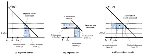
Figure 3.
Increments and decrements in the expected benefit and cost of Policy E over Policy C in period 2. The areas in the vertical blue stripes represent the increments and the horizontal blue stripes represent the decrements in (a) benefit, (b) cost, and (c) net benefit. The areas of the shaded triangles or squares represent the increments or decrements in the expected amount evaluated in period 0.
Why does Policy E achieve a larger cost reduction? In period 1, the user increases intake when observing and decreases it when observing to stabilize the benefit in the period. These behaviours can be seen simultaneously as an intertemporal reallocation of groundwater intake, which in turn affects the intertemporal allocation of groundwater stock and thereby unit pumping cost. The increase (decrease) in intake in period 1 increases (reduces) the unit pumping cost in period 2. This makes the relative price of groundwater in period 2 to period 1 higher (lower) than that of Policy C. Thus, transferring the intake from period 2 to period 1 or from period 1 to period 2 reduces the pumping cost in period 2. In other words, the intertemporal reallocation of groundwater intake, which occurs as a result of the stabilizing behaviour in period 1, generates a higher expected net benefit in Policy E through the cost reduction realized by the corresponding intertemporal reallocation of the unit pumping cost.
4.3.2. Policy R
From Equation (21), the user determines the intake to equate the marginal benefit with the sum of the unit cost and marginal user cost. Figure 4 illustrates these behaviours. In period 1, the user increases intake to a level more than Policy E when observing and decreases it to a level less than Policy E when observing . This destabilizes the total water use in period 1 and lowers the expected net benefit of the period. However, it achieves a much larger cost reduction in period 2 than that of Policy E and generates a higher total expected net benefit. This is why the behaviour described in Proposition 2 decreases the expected net benefit in the first period but increases it in the second period, and finally results in an increased total expected net benefit, as stated in Proposition 3.
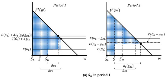
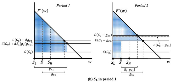
Figure 4.
User’s intake decisions and corresponding net benefits for Policies R and C. The areas in the vertical blue stripes represent the net benefits achieved by Policy R and the horizontal blue stripes represent those achieved by Policy C. The line segment that is declining to the right is the marginal benefit curve, . The horizontal lines represent the unit cost or the sum of the unit cost and marginal user cost.
In summary, the DRV is derived from users’ optimization to the changes in intertemporal cost allocations that occur as a reflection of their stabilizing behaviours. Users actively reallocate their groundwater intake intertemporally to save their pumping costs throughout the periods, thereby achieving a higher total benefit even in the case with uncertainty than in the case without uncertainty.
5. Responses to Different Environments
We examine, using some numerical illustrations, how each component of the TEV responds to different environments and how such reactions differ between the two regimes. To do so, we generalize the formulation of the DRV to models with an arbitrary number of stages. The derivations of the generalized DRV and the set of sample parameter values used in the illustrations are given by SI4 and SI5 in the Supporting Information.
Figure 5 shows how the AV, SSV, and DRV change as the number of stages increases. First, all values including the DRV increase but in different manners. The increment in the AV over s decreases as increases. This is because of users’ intertemporal levelling behaviour of groundwater within a given stock amount. The SSV increases linearly; the increment in the SSV is constant. In contrast, the increment in the DRV increases. This is because the impact of the intertemporal reallocation is transferred to the following stages through the corresponding changes in stock and cost. As a result, the share of the DRV in the DSV and TEV increases as increases. Second, the multiple-user regime exhibits lower values except for the SSV. In addition, the share of the DRV in the DSV and TEV is lower in the multiple-user regime. The results for the AV and SSV are consistent with the findings of the previous studies. For instance, Msangi and Hejazi [13] showed that suboptimal behaviours do not diminish the SV unless physical constraints on extraction capacities exist, but our results indicate that even if the constraints do not exist, the DSV can be impaired due to the decrease in the DRV. As we can see in (18), the users respond to surface water fluctuations by more than the amount of variations, but the magnitude is weaker in the multiple-user regime. The overexploitation in a suboptimal environment hinders users from fully utilizing reallocation opportunities.
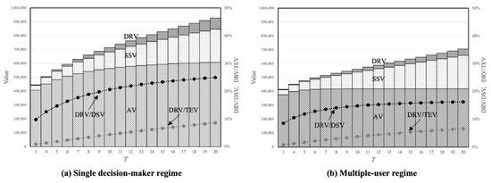
Figure 5.
Economic value of groundwater for different numbers of stages. The bar charts represent the values of the AV, SSV, and DRV, and the line graphs represent the DRV/DSV and DRV/TEV ratios.
Figure 6 shows how the SSV and DRV change as the variance of the surface water fluctuation increases. Both increase linearly; however, the slope of the DRV is smaller. This is because the DRV is a by-product of the stabilizing behaviour, and therefore utilizes fluctuations to a lesser extent than the SSV. Again, the slope of the DRV is smaller in the multiple-user regime. Figure 6 also shows how the SSV and DRV respond to different levels of , pumping cost elasticity to changes in stock level. The slope of the DRV increases as increases. This indicates a significant difference, with an implication from the existing studies that the elasticity has no effect on the SV since it is determined only by the risk premium in (4).
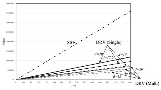
Figure 6.
SSV and DRV for different levels of variance in surface water fluctuation and of the elasticity of pumping costs.
Figure 7 shows how the SSV and DRV change as the value of the discount factor increases. First, in the single-decision-maker regime, both the AV and DRV increase as users give greater weight to the future. However, the increase in the AV comes from the behaviours of allocating more resources to the future on average irrespective of fluctuations. The increase in the DRV is also generated by similar behaviours but they are only related to the users’ stabilizing actions, not to the average intake amount. Second, the importance of the DRV in the DSV grows as the discount factor increases. Third, the multiple-user regime exhibits similar direction but with much smaller magnitude. This is because users overexploit more in earlier stages so that the pumping cost keeps rising due to the declining stock, which in turn leads to intake decreases over time [14]. The room for the intertemporal reallocation is limited in later stages so that the higher discount factor has only marginal impacts.
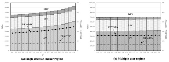
Figure 7.
Economic value of groundwater for different levels of the discount factor. The bar charts represent the values of the AV, SSV, and DRV, and the line graphs represent the DRV/SSV and DRV/TEV ratios.
6. Discussion
Unfortunately, the DRV has been overlooked even in studies conducted in dynamic contexts. As a result, these studies underestimate the magnitude of the SV and overestimate that of the SV.
This may cause serious practical drawbacks beyond purely theoretical issues. First, disregarding the DRV can underestimate the value of groundwater as an essential instrument for climate adaptation. The DRV augments the importance of groundwater, particularly in areas threatened by an unstable supply of surface water. Groundwater can provide those areas with greater economic benefits beyond its static stabilization effects. Our findings suggest such benefits are larger in areas requiring a longer perspective or facing a higher pumping cost elasticity. However, it is very likely that the management of just offsetting fluctuations, namely, what we call Policy E, has been conducted because it is the practice that scholars have proposed explicitly or implicitly.
Second, disregarding the DRV can underestimate the impact of a suboptimal environment on the stabilization function. Our findings show that overexploitation reduces the benefits even without the physical constraints. Proper regulations or collective actions are essential not only for avoiding resource exhaustion but also for fully leveraging the stabilization function. To address the issues in multiple-user environments, Provencher and Burt [29] proposed restrictions on individual extraction, pumping taxation, the licensing or permitting of wells, and collective management through water user associations. Burness and Brill [31] also discussed pumping tax and Gardner et al. [30] discussed a stock quota, a right assigning a share in groundwater stock. But these traditional measures are not sufficient to maximize the DRV, since it requires coordinated actions not only in levels but also in timing. Even if the average level of pumping is within the range of sustainable resource use, the timing of an increase or decrease is not harmonised, and users cannot derive the full value of dynamic reallocation. We therefore propose the real-time sharing of stock and extraction data as well as of the current magnitude of the DRV estimated by algorithms such as deep reinforcement learning. Local authorities or user associations can utilize these real-time data to facilitate effective harmonization.
7. Conclusions
7.1. Conclusions
In this study, we revisited the stabilization value of groundwater in a dynamic context. Different from the existing studies that have used a false specification of the SV and measured the DRV as part of the AV without noticing it, we explicitly detached it from AV and proposed a corresponding new composition of the TEV. Furthermore, we analysed the behavioural mechanisms of the DRV using a simple analytical model, where users respond to the surface water fluctuations by their groundwater intakes with greater magnitudes than the fluctuations themselves. Such behaviours arise from their optimization against changes in intertemporal cost allocations that occur as a reflection of the stabilizing behaviours.
In addition, we analysed how each component of the TEV responds to different environments. First, we found that the DRV and its share in the DSV and in the TEV increases as time horizon is prolonged and as users give greater weight to the future. Second, the more elastic the unit pumping cost is to changes in the groundwater level, the higher the DRV and its share in the DSV would be, whereas the SSV is unaffected. These findings show us how distinct the responses of the DRV to different environments are from those of the SSV and AV and justify the practical importance of distinguishing them in evaluations of the economic value of groundwater. Third, the DRV, and DSV, diminishes in a suboptimal environment with multiple users because overexploitation hinders users from fully utilizing reallocation opportunities. This is completely different from the findings of the existing literature that the SV stays unaffected even in a suboptimal environment unless there exist physical constraints on extraction capacities.
7.2. Limitations and Future Empirical Studies
Although the present paper did not apply actual water data, it is preferable to conduct empirical studies that incorporate the proposed approach in the economic valuation of the actual water environment. In doing so, there are some points that require further considerations. First, we used a stationary, temporally independent random variable for surface water fluctuations. This is because the typical situations that the current study addresses are those in which industrial or agricultural users tackle fluctuations in a relatively short period of time, for example, monthly. However, we can examine our findings in broadened environments, such as Markovian disturbances (e.g., [32,33]) or even in cases in which distributions are completely unknown. Examining the concrete impact of Markovian disturbances or unknown distributions on the DRV requires numerical simulations, for example, using deep reinforcement learning. However, considering the fundamental source of the DRV is optimization against changes in intertemporal cost allocations under stochastic environments, it is unconceivable that such specifications of the disturbance would deny the existence of the DRV itself as long as the model learning converges.
Second, although the present study used a relatively simple setting for hydrological processes, such as deterministic recharge, we can examine our framework under more complex interactions between precipitation, surface water flow, groundwater recharge, both natural and artificial, and attendant environmental externalities, such as land subsidence and saltwater intrusion [10,34,35,36]. In particular, climate-induced recharge variability has become increasingly important for the conjunctive management of surface and groundwater. Because variable recharge tends to amplify the system’s fluctuations, it is generally expected to increase the magnitude of the DRV. However, further numerical examination is required, especially to account for the effects of temporal lags. Furthermore, some recent studies are useful for computing the DRV in actual hydrological interactions. For example, the Multiple-Condition Fusion Neural Network (MCF-Net), proposed by Cui et al. [37] for subsurface characterization, as well as isotope-based runoff tracing approaches, such as those of Li et al. [38] and Lu et al. [39], enable the more accurate measurement and prediction of the interactions between surface water variability, irrigation, and groundwater recharge.
Third, a growing body of literature has simulated the optimized conjunctive management of surface water and groundwater using machine learning models [40,41]. It is preferable to deploy these models to examine the optimal dynamic reallocation under more complex configurations of actual water environments. In particular, conjunctive management requires multi-objective management to address inherently conflicting factors such as economic rationality and environmental externalities. Recent studies, for instance, the Localized Search Differential Evolution Algorithm (LS-DEA) proposed by Du et al. [42] and the multi-objective optimization scheduling model for cascade reservoirs developed by Liu et al. [43], can contribute to advancing such multi-objective optimization including the assessment of the DRV.
Supplementary Materials
The following supporting information can be downloaded at: https://www.mdpi.com/article/10.3390/w17202979/s1, SI1. Solution of the Two-stage Model. SI2. Proof of Proposition 1. SI3. Proof of Proposition 3. SI4. Generalization of DRV to Arbitrary Number of Stages. SI5. Parameter Values Used in the Numerical Illustration (References [44,45] are cited in the Supplementary Materials).
Author Contributions
Methodology, Z.Z.; Validation, Z.Z. and M.S.; Formal analysis, Z.Z.; Data curation, M.S.; Writing—original draft, Z.Z.; Writing—review & editing, M.S.; Supervision, M.S.; Funding acquisition, Z.Z. All authors have read and agreed to the published version of the manuscript.
Funding
This work was supported by JST SPRING (grant number: JPMJSP2114).
Data Availability Statement
The original data presented in the study are openly available in Zenodo at https://zenodo.org/records/13309130 (accessed on 14 October 2025).
Conflicts of Interest
The authors declare no conflicts of interest relevant to this study.
References
- Tsur, Y. The stabilization role of groundwater when surface water supplies are uncertain: The implications for groundwater development. Water Resour. Res. 1990, 26, 811–818. [Google Scholar] [CrossRef]
- Tsur, Y.; Graham-Tomasi, T. The buffer value of groundwater with stochastic surface water supplies. J. Environ. Econ. Manag. 1991, 21, 201–224. [Google Scholar] [CrossRef]
- Tsur, Y. The Economics of Conjunctive Ground and Surface Water Irrigation Systems: Basic Principles and Empirical Evidence from Southern California. In Decentralization and Coordination of Water Resource Management; Parker, D.D., Tsur, Y., Eds.; Natural Resource Management and Policy 10; Springer: Boston, MA, USA, 1997. [Google Scholar] [CrossRef]
- Ranganathan, C.R.; Palanisami, K. Modeling economics of conjunctive surface and groundwater irrigation systems. Irrig. Drain. Syst. 2004, 18, 127–143. [Google Scholar] [CrossRef]
- Gemma, M.; Tsur, Y. The stabilization value of groundwater and conjunctive water management under uncertainty. Rev. Agric. Econ. 2007, 29, 540–548. [Google Scholar] [CrossRef]
- Palanisami, K.; Gemma, M.; Ranganathan, C.R. Stabilisation value of groundwater in tank irrigation systems. Indian J. Agric. Econ. 2008, 63, 126–134. [Google Scholar] [CrossRef]
- Kakumanu, K.; Bauer, S. Conjunctive use of water: Valuing of groundwater under irrigation tanks in semiarid region of India. Int. J. Water 2008, 4, 87–104. [Google Scholar] [CrossRef]
- Nanthakumaran, A.; Palanisami, K. Assessment of the potential of groundwater supplementation by estimating the stabilization value of tank irrigation systems in Tamil Nadu, India. Trop. Agric. Res. 2011, 22, 84–93. [Google Scholar] [CrossRef]
- Palanisami, K.; Giordano, M.; Kakumanu, K.R.; Ranganathan, C.R. The stabilization value of groundwater: Evidence from Indian tank irrigation systems. Hydrogeol. J. 2012, 20, 933–941. [Google Scholar] [CrossRef]
- Kovacs, K.; Popp, M.; Brye, K.; West, G. On-farm reservoir adoption in the presence of spatially explicit groundwater use and recharge. J. Agric. Resour. Econ. 2015, 40, 23–49. [Google Scholar] [CrossRef]
- Kovacs, K.; West, G. The influence of groundwater depletion from irrigated agriculture on the tradeoffs between ecosystem services and economic returns. PLoS ONE 2016, 11, e0168681. [Google Scholar] [CrossRef]
- MacEwan, D.; Cayar, M.; Taghavi, A.; Mitchell, D.; Hatchett, S.; Howitt, R. Hydroeconomic modeling of sustainable groundwater management. Water Resour. Res. 2017, 53, 2384–2403. [Google Scholar] [CrossRef]
- Msangi, S.; Hejazi, M. How stable is the stabilization value of groundwater? Examining the behavioral and physical determinants. Water Resour. Econ. 2022, 38, 100195. [Google Scholar] [CrossRef]
- Zhang, Z.Y.; Sato, M. Conjunctive surface water and groundwater management in a multiple user environment. Environ. Econ. Policy Stud. 2024, 26, 803–841. [Google Scholar] [CrossRef]
- Tsur, Y.; Park, H.; Issar, A. Fossil groundwater resources as a basis for arid zone development? Int. J. Water Resour. Dev. 1989, 5, 191–201. [Google Scholar] [CrossRef]
- Dinar, A.; Tsur, Y. The Economics of Water Resources: A Comprehensive Approach; Cambridge University Press: Cambridge, UK, 2021; pp. 115–132. [Google Scholar] [CrossRef]
- Quintana-Ashwell, N.E.; Gholson, D.M. Optimal Management of Irrigation Water from Aquifer and Surface sources. J. Agric. Appl. Econ. 2022, 54, 496–514. [Google Scholar] [CrossRef]
- Bruno, E.M.; Hagerty, N.; Wardle, A.R. The Political Economy of Groundwater Management: Descriptive Evidence from California. In American Agriculture, Water Resources, and Climate Change; Libecap, G.G., Dinar, A., Eds.; University of Chicago Press: Chicago, IL, USA, 2023. [Google Scholar]
- Cooley, D.; Smith, S.M. Center Pivot Irrigation Systems as a Form of Drought Risk Mitigation in Humid Regions. In American Agriculture, Water Resources, and Climate Change; Libecap, G.G., Dinar, A., Eds.; University of Chicago Press: Chicago, IL, USA, 2023. [Google Scholar]
- Hrozencik, R.A.; Gardner, G.; Potter, N.; Wallander, S. Irrigation Organizations: Groundwater Management; Economic Research Service, Economic Brief 34; U.S. Department of Agriculture: Washington, DC, USA, 2023. [Google Scholar] [CrossRef]
- Zhao, J.; Hendricks, N.P.; Li, H. Groundwater Institutions in the Face of Global Climate Change. Annu. Rev. Resour. Econ. 2024, 16, 125–141. [Google Scholar] [CrossRef]
- Harris, L. Farmer response to policy induced water reductions: Evidence from the Colorado River. J. Environ. Econ. Manag. 2024, 25, 102986. [Google Scholar] [CrossRef]
- Hrozencik, A.; Perez-Quesada, G.; Donahue, H. The development and current challenges of irrigated agriculture in the western U.S. Agric. Water Manag. 2025, 215, 109474. [Google Scholar] [CrossRef]
- Cuthbert, M.O.; Gleeson, T.; Moosdorf, N.; Befus, J.; Lehner, B. Global patterns and dynamics of climate–groundwater interactions. Nat. Clim. Change 2019, 9, 137–141. [Google Scholar] [CrossRef]
- Burt, O.R. The economics of conjunctive use of ground and surface water. Hilgardia 1964, 36, 31–111. [Google Scholar] [CrossRef]
- Knapp, K.C.; Olson, L.J. The economics of conjunctive groundwater management with stochastic surface supplies. J. Environ. Econ. Manag. 1995, 28, 340–356. [Google Scholar] [CrossRef]
- Joodavi, A.; Zare, M.; Mahootchi, M. Development and application of a stochastic optimization model for groundwater management: Crop pattern and conjunctive use consideration. Stoch. Environ. Res. Risk Assessment. 2015, 29, 1637–1648. [Google Scholar] [CrossRef]
- Gisser, M.; Sánchez, D.A. Competition versus optimal control in groundwater pumping. Water Resour. Res. 1980, 16, 638–642. [Google Scholar] [CrossRef]
- Provencher, B.; Burt, O. Approximating the optimal groundwater pumping policy in a multiaquifer stochastic conjunctive use setting. Water Resour. Res. 1994, 30, 833–843. [Google Scholar] [CrossRef]
- Gardner, R.; Moore, M.R.; Walker, J.M. Governing a groundwater commons: A strategic and laboratory analysis of western water law. Econ. Inq. 1997, 35, 218–234. [Google Scholar] [CrossRef]
- Stuart, B.H.; Brill, T.C. The role for policy in common pool groundwater use. Resour. Energy Econ. 2001, 23, 19–40. [Google Scholar] [CrossRef]
- Srikanthan, R.; McMahon, T.A. Stochastic Generation of Rainfall and Evaporation Data; Australian Water Resources Council, Technical Report 84; Department of Resources and Energy: Canberra, Australia, 1985. [Google Scholar]
- Srikanthan, R.; McMahon, T.A. Stochastic generation of annual, monthly and daily climate data: A review. Hydrol. Earth Syst. Sci. 2001, 5, 653–670. [Google Scholar] [CrossRef]
- Mounira, Z.; Naima, B. Efficiency of Artificial Groundwater Recharge, Quantification Through Conceptual Modelling. Water Resour. Manag. 2020, 34, 3345–3361. [Google Scholar] [CrossRef]
- Reznik, A.; Dinar, A.; Bresney, S.; Forni, L.; Joyce, B.; Wallander, S.; Bigelow, D.; Kan, I. Institutions and the economic efficiency of managed aquifer recharge as a mitigation strategy against drought impacts on irrigated agriculture in California. Water Resour. Res. 2022, 58, e2021WR031261. [Google Scholar] [CrossRef]
- Díaz-Nigenda, J.J.; Morales-Casique, E.; Carrillo-García, M.; Alberto Vázquez-Peña, M.; Escolero-Fuentes, O. Importance of Aquitard Response Time for Groundwater Management in Multi-Aquifer Systems Subject to Land Subsidence. Water Resour. Manage. 2023, 37, 5367–5378. [Google Scholar] [CrossRef]
- Cui, Z.; Chen, Q.; Luo, J.; Ma, X.; Liu, G. Characterizing subsurface structures from hard and soft data with multiple-condition fusion neural network. Water Resour. Res. 2024, 60, e2024WR038170. [Google Scholar] [CrossRef]
- Li, R.; Xiaoyu, Q.; Longhu, C.; Guofeng, Z.; Gaojia, M.; Yuhao, W.; Enwei, H.; Yinying, J.; Qinqin, W.; Wenmin, L. Hydrological processes in continental valley basins: Evidence from water stable isotopes. CATENA 2025, 259, 109314. [Google Scholar] [CrossRef]
- Lu, S.; Zhu, G.; Qiu, D.; Li, R.; Jiao, Y.; Meng, G.; Lin, X.; Wang, Q.; Zhang, W.; Chen, L. Optimizing irrigation in arid irrigated farmlands based on soil water movement processes: Knowledge from water isotope data. Geoderma 2025, 460, 117440. [Google Scholar] [CrossRef]
- Safavi, H.R.; Enteshari, S. Conjunctive use of surface and ground water resources using the ant system optimization. Agric. Water Manag. 2016, 173, 23–34. [Google Scholar] [CrossRef]
- Rezaei, F.; Safavi, H.R.; Mirchi, A.; Madani, K. f-MOPSO: An alternative multi-objective PSO algorithm for conjunctive water use management. J. Hydro-Environ. Res. 2017, 14, 1–18. [Google Scholar] [CrossRef]
- Du, K.; Shucheng, Y.; Wei, X.; Feifei, Z.; Huanfeng, D. A novel optimization framework for efficiently identifying high-quality Pareto-optimal solutions: Maximizing resilience of water distribution systems under cost constraints. Reliab. Eng. Syst. Saf. 2025, 261, 111136. [Google Scholar] [CrossRef]
- Liu, G.; Enhui, J.; Donglin, L.; Jieyu, L.; Yuanjian, W.; Wanjie, Z.; Zhou, Y. Annual multi-objective optimization model and strategy for scheduling cascade reservoirs on the Yellow River mainstream. J. Hydrol. 2025, 659, 133306. [Google Scholar] [CrossRef]
- Basar, T. Dynamic Noncooperative Game Theory; Academic Press: London, UK, 2012. [Google Scholar]
- Bellman, R. On the Theory of Dynamic Programming. Proc. Natl. Acad. Sci. USA 1952, 38, 716–719. [Google Scholar] [CrossRef]


Disclaimer/Publisher’s Note: The statements, opinions and data contained in all publications are solely those of the individual author(s) and contributor(s) and not of MDPI and/or the editor(s). MDPI and/or the editor(s) disclaim responsibility for any injury to people or property resulting from any ideas, methods, instructions or products referred to in the content. |
© 2025 by the authors. Licensee MDPI, Basel, Switzerland. This article is an open access article distributed under the terms and conditions of the Creative Commons Attribution (CC BY) license (https://creativecommons.org/licenses/by/4.0/).