Article

Comparison of Pluvial Flooding Modeling Software Applied in Highly Urbanized Settlements Using the Case of Lake Ganzirri

by
José Javier Serrano Chano
1,2,*,
Giuseppina Brigandi
2 and
Giuseppe Tito Aronica
2
1
University School for Advanced Studies IUSS Pavia, 27100 Pavia, Italy
2
Department of Engineering, University of Messina, 98122 Messina, Italy
*
Author to whom correspondence should be addressed.
Water 2025, 17(20), 2978; https://doi.org/10.3390/w17202978
Submission received: 30 July 2025 / Revised: 26 September 2025 / Accepted: 13 October 2025 / Published: 15 October 2025

Abstract

The rising urbanization and climate change have increased pluvial flood risks, especially in highly urbanized areas. This study focuses on the Lake Ganzirri area in Messina, Italy, where street-level floods have raised concerns for infrastructure resilience and public safety. This study aims to explore how to effectively represent key urban features, emphasizing buildings and low-impact development/sustainable urban drainage systems (LID/SUDS). For the buildings, a combination of referred approaches to represent buildings is compared against the widely used method to represent buildings as voids in a 2D mesh, ignoring them in the water balance calculations. For the LID/SUDS control elements, a 2D representation is presented and compared against the widely used 1D approach to model such elements. The study uses three well-known software packages—EPA-SWMM 5.2, HEC-RAS 6.2, and InfoWorks ICM 2021.9—applied to the Lake Ganzirri area, to explore the representation of buildings using the building void method (available in InfoWorks ICM 2021.9) against the proposed method (in HEC-RAS 6.2) to replicate runoff flow over a 2D model of a highly urbanized area. From scenario S0, three more scenarios were derived: S1 (S0 with pluvial drainage network), S2 (S1 with LID/SUDS control elements), and S3 (S0 with 2D representation of LID/SUDS), which were then compared against using four comparison schemes. Results show that the proposed method for representing buildings computed the propagation of the runoff comparable to when the building void method is used, with some shortcomings regarding mesh adjustments and computational times. Regarding the 2D representation of LID/SUDS, the effects were unperceivable on water depth maps (reduction in water depths of 1.5 mm on average for all the rainfall events). Still, they were reflected in the increase of 62% of the infiltration volume on average of all the rainfall scenarios and a decrease of 9.1% of water flowing outside the 2D area, therefore replicating the effect of capturing water.

1. Introduction

Since 2007, more people have been living in cities than in rural areas for the first time [1] (p. 609). This accelerated, and often unplanned, urban expansion alters the natural water cycle due to the presence of concrete, asphalt, and hard materials for buildings, roads, and general public infrastructure in conventional urban settlements [2] (p. 138). In addition, human-induced climate change effects have resulted in the alteration of spatiotemporal patterns of rainfall, which, in some areas, translates into stronger and more frequent extreme rainfall events [3] (p. 4). The impermeabilization of the landscape reduces the capacity of rainfall to infiltrate into the land and evaporate towards the atmosphere, therefore increasing the amount that slides down slopes as runoff on impermeable areas [4] (p. 2).
Studies in urbanization recognize the value of highly dense urban settlements as essential services (water, electricity, gas, transport, facilities, solid waste management, etc.) are delivered in smaller areas, reducing investments, operational costs, and efficiency in general [5] (p. 383). Nevertheless, higher population densities present disadvantages from an urban water management perspective as surface runoff volumes grow with the urban expansion, facilitating floods due to the collapse of existing drainage pipe networks or overflowing urban streams [6] (p. 380), threatening larger numbers of people.
Understanding floods in urban areas requires a comprehensive understanding of the water cycle in urban catchments, which can be defined as a highly heterogeneous mix of natural and artificial landscapes with a mix of natural and human-induced activities interacting with each other and with rainfall [7] (p. 64). Understanding this complexity can help further develop the body of knowledge regarding climate change resilience, flood prediction and monitoring, urban planning, and adaptive management practices, which often require the development of comprehensive flood models [8]. Most studies in urban settlements focus on catchment-size applications, using both gridded and non-gridded approaches, with fewer small-size applications (grid elements < 20 × 20 m) and small temporal resolutions (less than a day) [7] (p. 70).
Highly urbanized areas can pose a significant challenge when simulating rainfall runoff responses, as hydrological and hydraulic responses change from one place to another due to the presence of buildings, different land uses, and existing infrastructure, which generally alter the runoff flow over the surface. The complexity increases when LID/SUDS strategies are taken into consideration.
For flood risk management, specialized software usually combines a lumped model (1D approach) with a 2D domain for flood mapping [9]. For fluvial flooding, the 1D approach generates a hydrograph that turns into the boundary conditions (source points) of the 2D model. For non-fluvial floods (i.e., pluvial), the application of the direct rainfall method (DRM), also referred to as rain-on-grid (RoG), has been widely adopted to represent hydrological and hydrodynamic processes on a 2D domain [10]. This method can be used in urban catchments to configure fully integrated 2D models, where the runoff flowing over the surface, the overflow from the nodes in a drainage system, and infiltration processes of the urban water cycle are important [11] (p. 3).
The selection of modeling software for urbanized areas depends on what part of the urban water cycle will be represented, the objectives of the modeling itself, the level of detail of the output required, input data availability, the existence of observational data, and the scale of the study area.
Software such as InfoWorks ICM 2021.9 has been developed to study the interaction of rural and urban settlements. Therefore, it has tools to represent natural catchments, river streams, and urban features (buildings, roads, permeable and impermeable areas, and pipe networks) on a 2D domain and run RoG models and 1D/2D interaction models, which are widely used in urban hydrology studies. It also provides tools to explore the implementation of LID/SUDS objects (low-impact developments/sustainable urban drainage systems) at the catchment level using a lumped approach. In contrast, HEC-RAS 6.2, a free software, is commonly used for modeling catchments and river streams, including overflow and rain-on-grid modeling, which is a widely used approach in urban settlements. Additionally, EPA-SWMM 5.2, another well-known free software, is used for designing pluvial networks, employing a lumped approach to estimate the outflow of a catchment based on hydrological features, infiltration characteristics, and the implementation of LID/SUDS objects at the catchment level (lumped approach).
Ref. [11] introduces a solid list of case studies using the RoG method on a catchment at different scales, stressing that the drainage system becomes relevant when the urban catchment scale is smaller. In its case study (3800 Ha), the representation of buildings as flow barriers (equivalent to the building block method) and as highly rough surfaces (equivalent to the building resistance method) was also explored using HEC-RAS 6.2. The water depth maps presented problems in both representations of buildings. When representing them as flow barriers, the building’s perimeter was surrounded by a tall layer of water; when considering them as a highly rough surface, some buildings were fully covered with water. No further discussion about these results was presented, and the argument that the changes in the building representation did not have any effect on the resulting hydrographs or computational times closed the section explaining the buildings.
The study conducted in [12] describes a modeling approach, referred to as 1D/2D coupling, similar to the one described by [9], focused on a case study that includes peri-urban and urban areas. It is argued that 1D models are efficient at simulating the response of drainage networks during a heavy rainfall event, but struggle to represent accurately the presence of key urban features, especially buildings. The study presents an approach to couple a 1D drainage network model to a 2D domain to obtain the flow propagation of collapsing nodes at street-level, considering them as source points of flow. Therefore, the outputs of the 1D model are the boundary conditions for the 2D model.
The importance of the integrated approach is evident at this point. However, including LID/SUDS control elements on 2D domains remains unexplored. Studies regarding LID/SUDS implementation focus on evaluating its performance and benefits, selecting elements, and optimizing area assignment [13,14,15]. These types of studies are based on the effects of the presence of LID/SUDS control elements using EPA-SWMM 5.2 to model their effects (1D approach). Nevertheless, none of them explored the impacts of the spatial distribution on the runoff propagation (2D approach) or used a coupled approach to represent them using a 1D approach, and the outputs were modeled on a 2D domain [16,17].
In a world where information technology has leveraged improvements of geospatial techniques to obtain high-quality data to use in spatially distributed models [18] (p. 22), the level of detail comes with larger computational requirements for the calculations, therefore, longer simulation times. Consequently, this study details the mesh, hardware, and software used and adjustments to the 2D domain on a 100 Ha case study to explore the required simulation times for a detailed representation of a highly urbanized settlement.
The present study focuses on the detailed representation of key urban features (buildings, roads, permeable and impermeable areas, pipe networks, and LID/SUDS objects) that are crucial for the movement of water within an urban settlement in pluvial flood analysis, with an emphasis on buildings and the implementation of LID/SUDS elements. The aims of this study are proposing a method to represent buildings on a 2D domain and compare it with the widely used building void method, to explore the effects on the propagation of the runoff on a 2D domain when implementing LID/SUDS control elements as part of the 2D domain, and compare the outcomes with the regular representation of such elements using a 1D approach.

2. Materials and Methods

The present study models the same case study employing a lumped model for each urban sub-catchment (1D approach), and a rain-on-grid (RoG) model, also known as the fully hydrodynamic approach, direct rainfall method, hydrodynamic rainfall-runoff model, or hydro-inundation model, which was selected for its suitability in analyzing rainfall falling onto and flowing on 2D surfaces (2D approach) [9] (pp. 1–2).
The RoG model has become a state-of-the-art method for studying floods, mainstreaming its use in open-source and commercial software programs worldwide [10]. A description of the method and examples of application can be found in [19,20]. The rainfall input data were Chicago-style hyetographs for different return periods.
The surroundings of the study area, Lake Ganzirri, were modeled to assess the surface’s hydrologic and hydraulic response to rainfall events in a highly urbanized domain. In addition, a proposed drainage system and LID/SUDS strategies were also modeled.
Since this study focuses on modeling highly urbanized areas, three different and well-known software programs were used to construct a model of the urban features on a mesh to represent the status quo of the case study and explore the impacts of implementing a drainage system in the area and LID/SUDS strategies. The results of different simulation scenarios of Lake Ganzirri’s surroundings were compared and described further.

2.1. Study Area

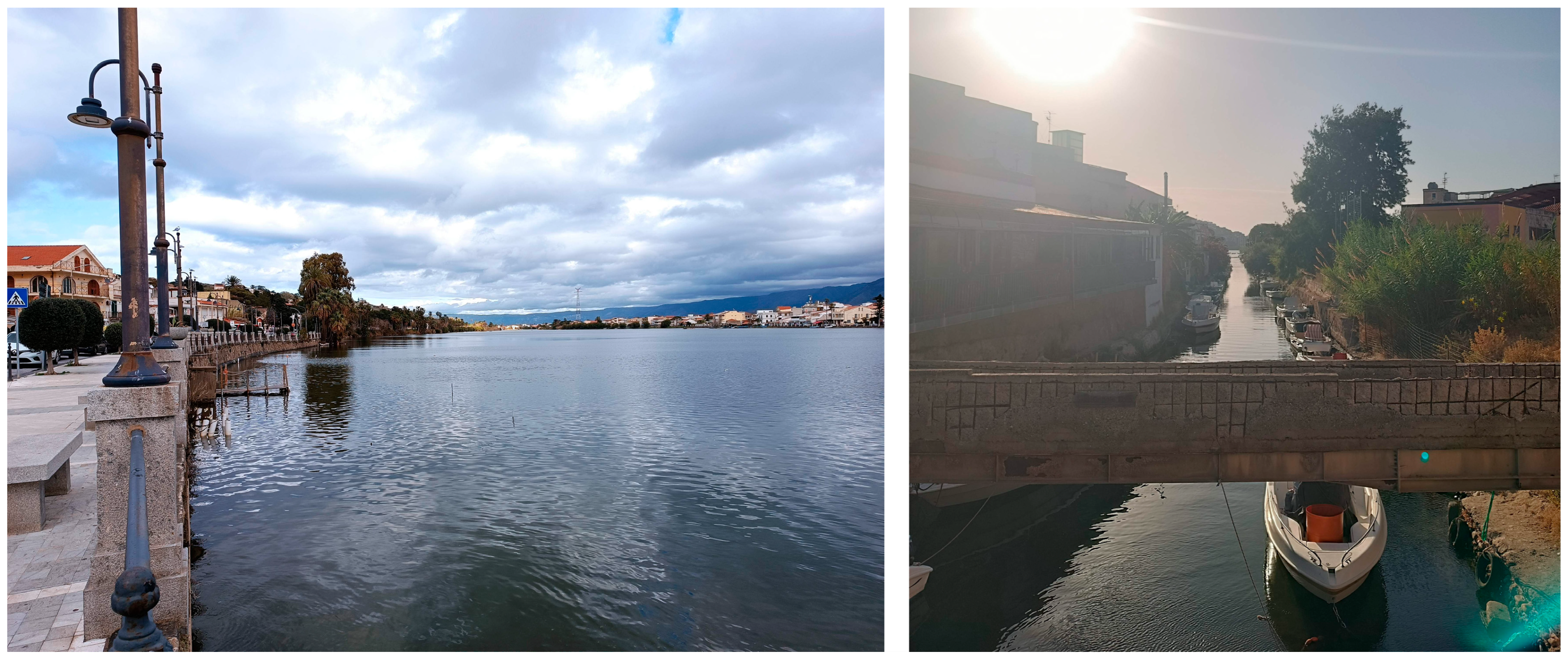
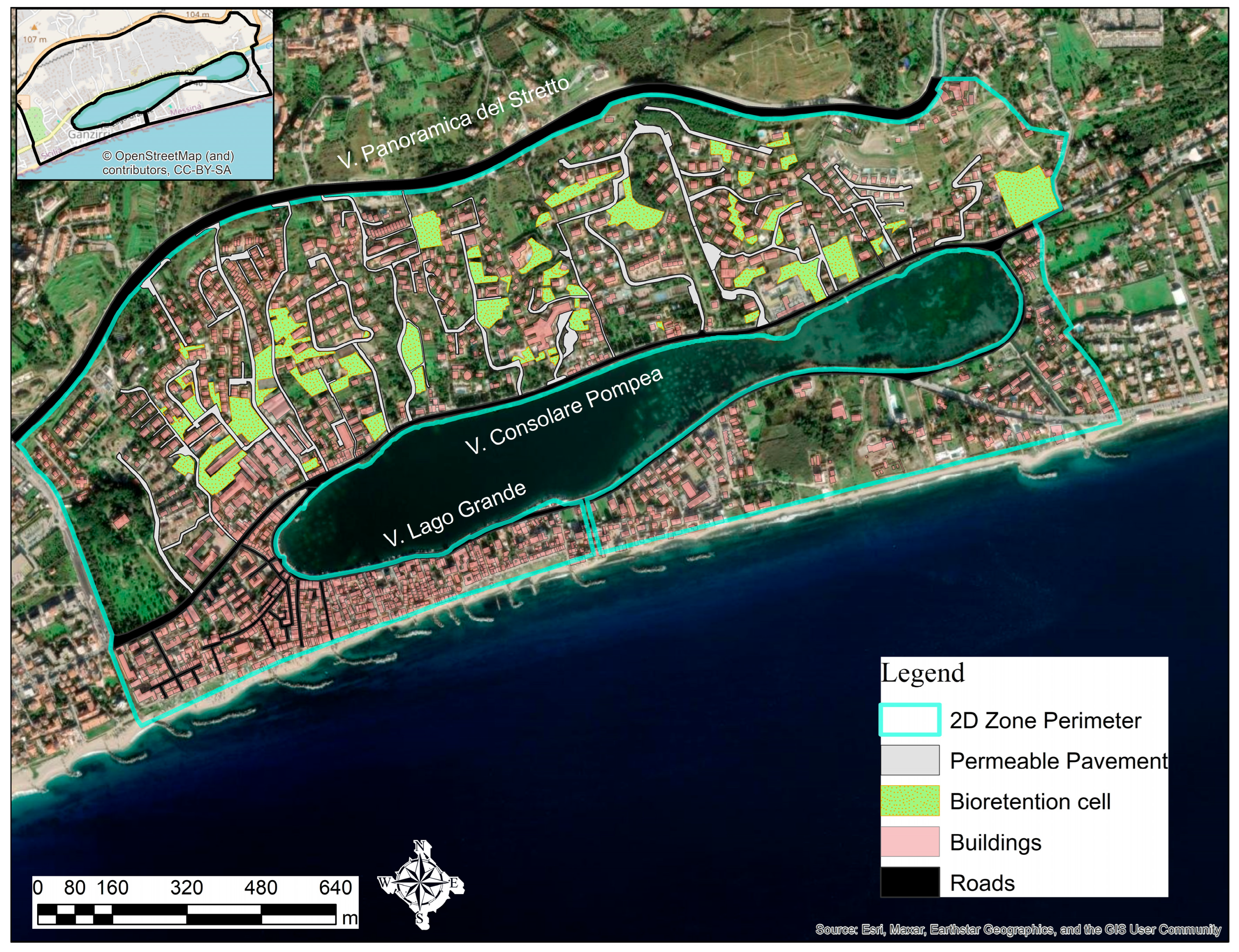
Lake Ganzirri is located on the northeastern tip of Sicily in Italy. It is a long, narrow, brackish coastal lagoon part of the Cape Peloro coastal lagoon system, which is connected to the Ionian Sea and the Lake Faro, which is also connected to the Ionian Sea and the Tyrrhenian Sea [21] (p. 8). The area surrounding the Lake of Ganzirri encompasses natural and man-made features (Figure 1 and Figure 2). There are extensive coastal lowlands and sea dunes around the lake and extensive and expanding human habitation, with Ganzirri and Torre Faro being the most relevant urban settlements. Two main roads surround the lake, Via Consolare Pompea (northern side) and Via Lago Grande (southern side).
The elevation along the roads surrounding the lake fluctuates from 0.60 to 3.50 m.a.s.l. in Via Consolare Pompea and from 0.40 to 2.40 m.a.s.l. in Via Lago Grande [22] (pp. 98–99). The area between Via Consolare Pompea and Panoramica dello Stretto has become attractive for residential complexes with small private green spaces. The study area (excluding the lake) covers 154.92 Ha and ranges from −0.25 to 190 m.a.s.l. along the coast of the Mediterranean Sea and Via Panoramica del Stretto, respectively.
There is an encasement along the perimeter of Lake Ganzirri and a wide channel that connects it with the Ionian Sea, as shown in Figure 2. A set of side drains connected to the lake discharged runoff water directly without any treatment, dismissing the need for a functional drainage network in the area. These side drains were the main way to discharge runoff from Via Consolare Pompea until October 2000, when the European Directive established a framework for community action on water policies with articles related to the prevention of the deterioration of water bodies’ quality by diffuse pollution [23]. The outlets were blocked to avoid direct discharge, leaving Via Consolare Pompea and Via Lago Grande highly susceptible to floods due to rainwater, as no formal drainage network was in place. In 2015, Lake Ganzirri became part of the “Morpho-tectonic system of Cape-Peloro-Lake Ganzirri” geosite due to its uniqueness and scientific value [21] (p. 8).
Despite Lake Ganzirri’s importance, it faces threats at different levels due to the accelerated urbanization of its surroundings, like the impermeabilization of the landscape, increasing floods due to rainwater runoff, and the risk of pollution caused by diffuse sources such as vehicular traffic. Therefore, hydrological/hydraulic models can support decision-making processes for future interventions aiming to comply with directives and mitigate future threats due to climate change.

2.2. Software and Hardware

The case study of Lake Ganzirri was modeled using HEC-RAS 6.2, InfoWorks ICM 2021.9, and EPA-SWMM 5.2. The Hydrologic Engineering Center’s River Analysis System (HEC-RAS), developed and distributed freely by the U.S. Army Corps of Engineers, was initially designed for 1D modeling but expanded its features to a 2D domain from the 5.0 version onwards [24] (p. 2). It computes the hydrological/hydraulic response of an area exposed to rainfall events without requiring the delimitation of catchments, as topographical features are included as input. A physically based approach is used to solve two-dimensional Shallow Water Equations over a mesh populated with buildings and roads’ presence, land, and soil cover data [25] (p. 186). It is commonly used for river and floodplain modeling, mainly in natural areas, and it can model hydraulic structures such as bridges, walls, culverts, etc. Version 6.5 (launched in November 2024) has added pipe network features, enabling it to simulate the interaction between a drainage network and a 2D domain. However, it presented problems recognizing a soil layer with different characteristics (buildings, roads, permeable and impermeable areas). Therefore, version 6.2 was preferred for this study because the soil layer could include various land uses.
Innovyze’s (Autodesk) InfoWorks ICM 2021.9 is a commercial software package for integrated hydrological/hydraulic modeling (1D, 2D, and 1D–2D interaction). It was designed to analyze the interaction between urban and rural environments. Therefore, it can manage complex systems with natural streams, urban drainage networks, open channels, sustainable urban drainage system (SUDS) objects, and floodplain areas. It has specific features for urban water and risk management.
The Environmental Protection Agency—Stormwater Management Model (EPA-SWMM 5.2) is an open-source software designed for single-event or long-term simulations of rainfall-runoff models and water quality, primarily for urban areas but not limited to them. It can handle drainage networks for pluvial flooding, open channels of different shapes, special elements (inlet drains, storage and treatment units, pumps, etc.), and SUDS objects. However, it does not have 2D features. The preferred version for this study was EPA-SWMM 5.2. It requires catchment delimitation and hydrological data when designing drainage systems and evaluating SUDS’ impacts on a catchment’s outflow. This is done using a lumped model approach that calculates a catchment’s outflow based on the rainfall input, hydrological features, proportion of areas used for SUDS implementation, and SUDS object parameters. A catchment’s outflow must be connected to a node and link system, representing a drainage system. The hydraulic calculations are performed through the node-link system, solving the St. Venant equations of a one-dimensional flow [26] (pp. 35–36).
InfoWorks ICM 2021.9 can import an EPA-SWMM 5.2 model via specific tools to replicate the catchment delimitation, hydrological features, and rainfall events in a model group. However, this feature was not applied in this study, as the aim was to compare the functionality of each software to represent highly urbanized areas and SUDS implementation.
Two computers were used for the present study. Table 1 summarizes their characteristics so the reader can have a reference on how commercial computers (laptop 1 = conventional laptop; laptop 2 = “gamer” laptop) perform running simulations of a highly urbanized area of approximately 100 Ha.
All three software programs are physically based on the Shallow Water Equations (SWEs), the most popular mathematical model for calculating water depth and speed at different times given a rainfall input [27] (p. 1).

2.3. Simulation Scenarios and Comparisons

Given the lack of observational data at street level of water depth during pluvial floods in the study area, a detailed 2D model was created using InfoWorks ICM 2021.9 and taken as the reality for this study. This reference model includes the limitations of no functional pluvial drainage system and blocked runoff discharge into Lake Ganzirri. It was carefully constructed using the actual geometry of buildings (no geometry simplification applied), accounting for the presence of vegetated areas, refinement of the mesh on roads, and carefully selected parameters to represent the different land uses. The InfoWorks model aimed to describe the runoff flow over various surfaces and around buildings in the real case study.
From the reference model in InfoWorks ICM 2021.9 (S0), three simulation scenarios were derived: (S1) implementation of a pluvial drainage system, (S2) a pluvial drainage system in combination with LID/SUDS elements, (S3) implementation of LID/SUDS only. Then, EPA-SWMM 5.2 and HEC-RAS 6.2 were used to construct models following a 1D or 2D approach to explore the representation of key urban features between commercial and free options of modeling software programs.
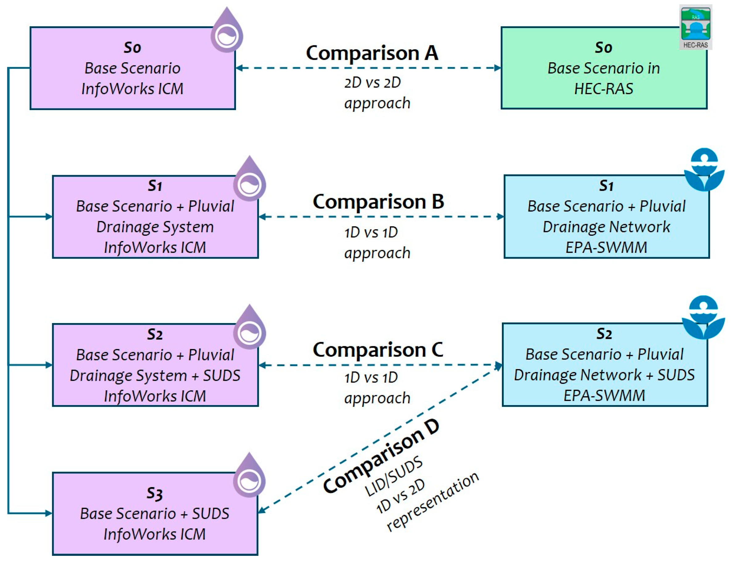
This study uses the simulation scenarios constructed in InfoWorks ICM 2021.9, HEC-RAS 6.2, and EPA-SWMM 5.2 with the following comparison schemes (Figure 3):
  • Comparison A: This scheme explored the representation of a highly urbanized settlement in a 2D fashion using as much detail as possible. InfoWorks ICM 2021.9 was used to adopt the building void method to represent buildings, and HEC-RAS 6.2 was used for the proposed method in this paper, as it is not possible to deactivate cells of the mesh in this software. The effects of the different representations of buildings are explored in this comparison scheme.
  • Comparison B: This scheme compares a simulated scenario with a proposed pluvial drainage system modeled using InfoWorks ICM 2021.9 and EPA-SWMM 5.2 with a 1D approach. This section explored the differences in using a lumped approach on both software packages. The pluvial drainage system was suggested to drain the runoff of the urbanized area between Via Consolare Pompea and Panoramica del Stretto.
  • Comparison C: We explored implementing LID/SUDS elements using incorporated tools in InfoWorks ICM 2021.9 and EPA-SWMM 5.2, which are only available using a 1D approach. A drainage system is required. Therefore, we used the same simulation scenario for comparison B, adding LID/SUDS elements.
  • Comparison D: This scheme compares LID/SUDS objects using EPA-SWMM 5.2 and InfoWorks incorporated tools, limited to a 1D approach, and a 2D representation using polygons with adapted meshing, infiltration, and roughness characteristics. This scheme will explore the representation of LID/SUDS control elements directly in the 2D domain, rather than as part of a 1D/2D coupling. The 2D representation was compared to the widely used 1D representation, and the effects on both outcomes were analyzed.

2.4. Comparison Scheme’s Methodology

Each comparison scheme was modeled using a pair of software packages using a 1D or 2D approach as described before. Comparison D is a special case, which was used to assess the differences in representation of LID/SUDS elements using a 1D and 2D approach. The results of the models were compared as detailed in Table 2.
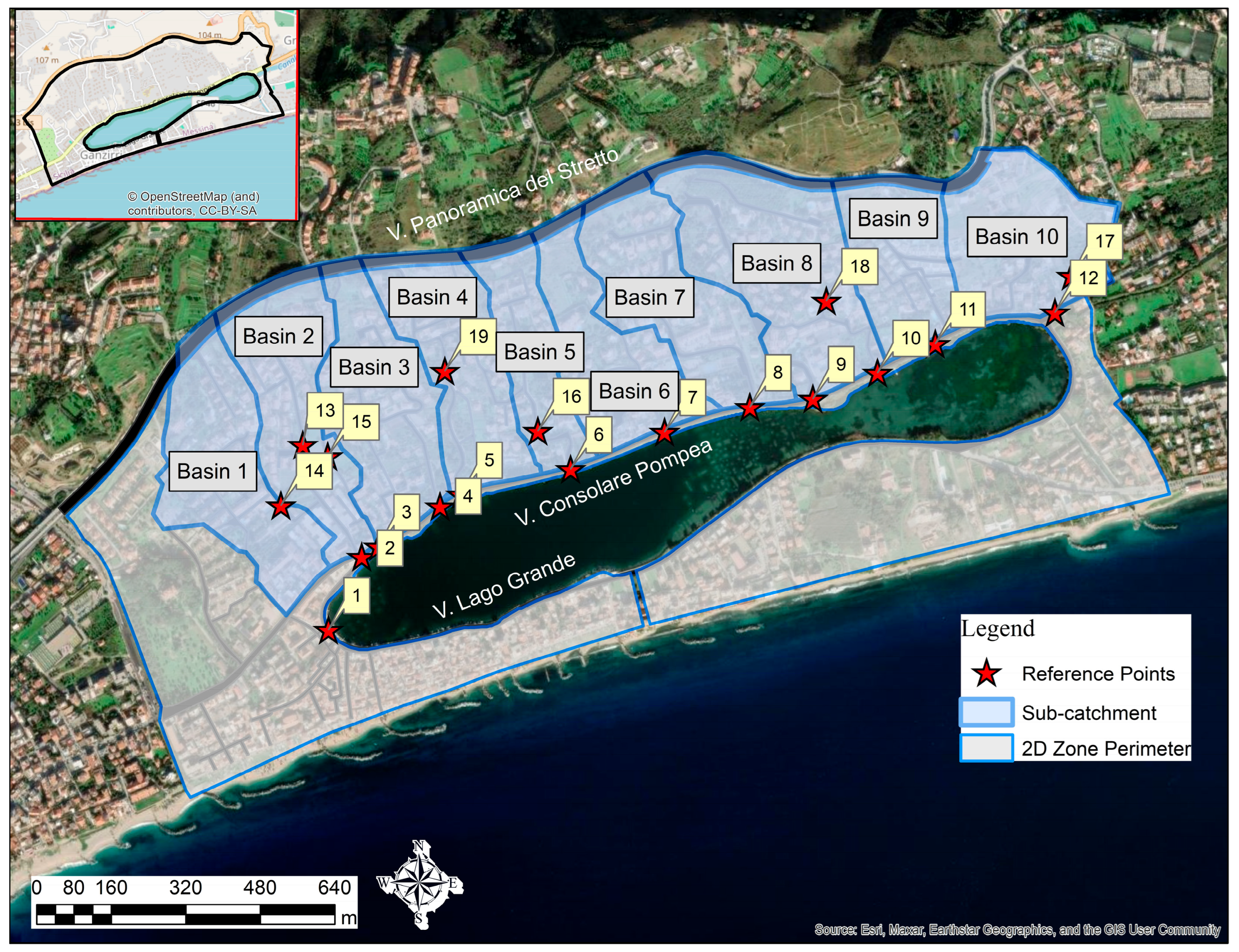
The statistics of the 2D simulation were extracted from each software. HEC-RAS 6.2 has a tool to display the statistics from the results section. On the other hand, InfoWorks ICM 2021.9 required exporting the maximum depth and speed results as rasters and applying GIS tools to calculate the statistics. A mesh element with a water depth greater than 1 cm was considered inundated for the inundated area calculation. The volume balance report is extracted from each simulation’s log results. The max depth and speed values from the reference points were extracted using InfoWorks’ result analysis tool fed by results points (2D) created with the coordinates of the reference points across the study area (Figure 4).
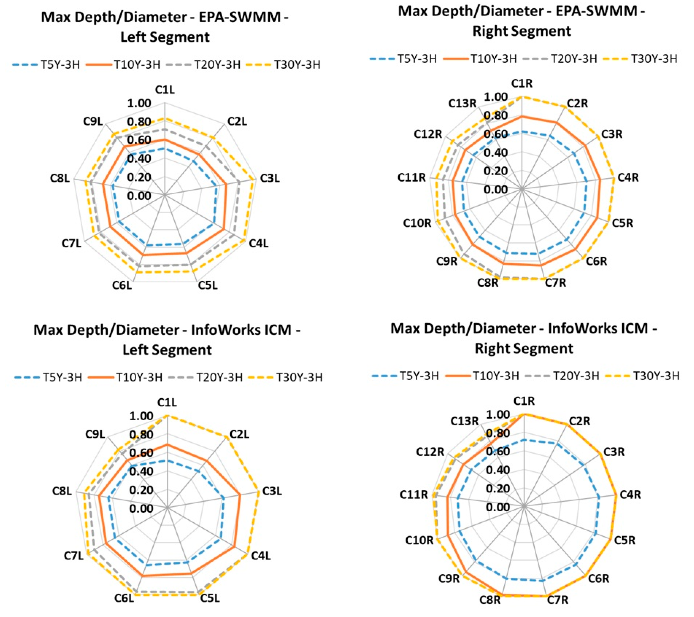
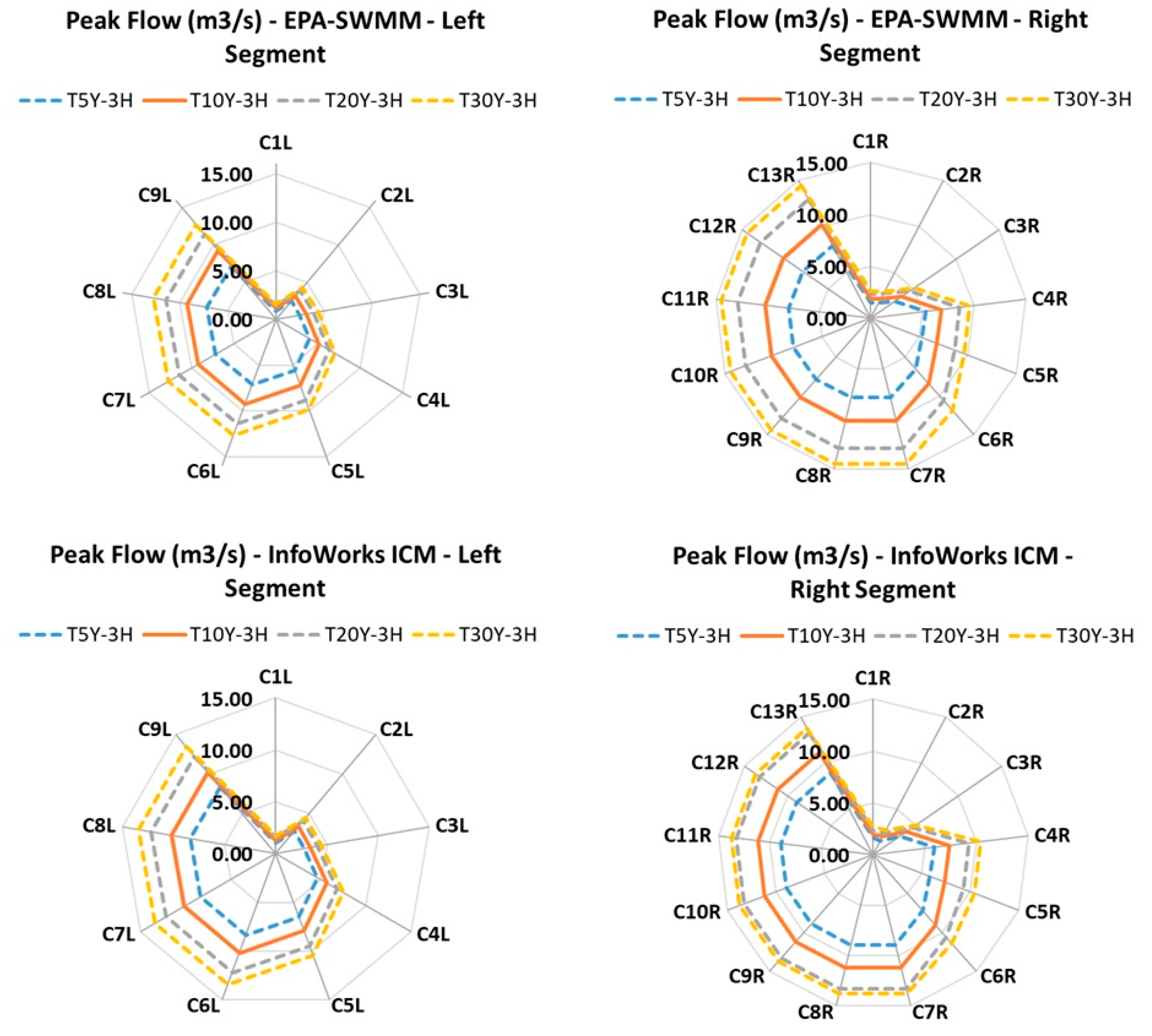
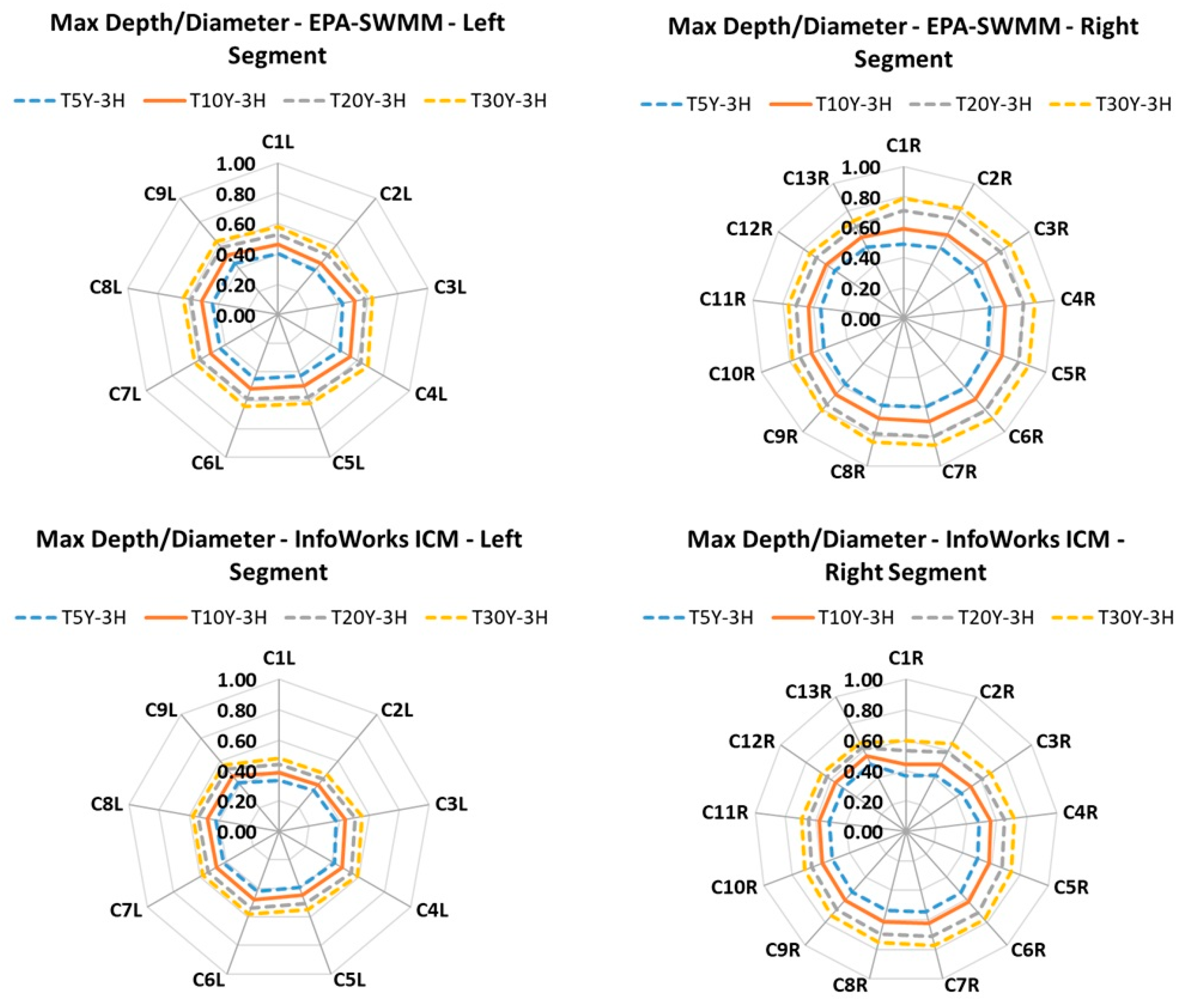
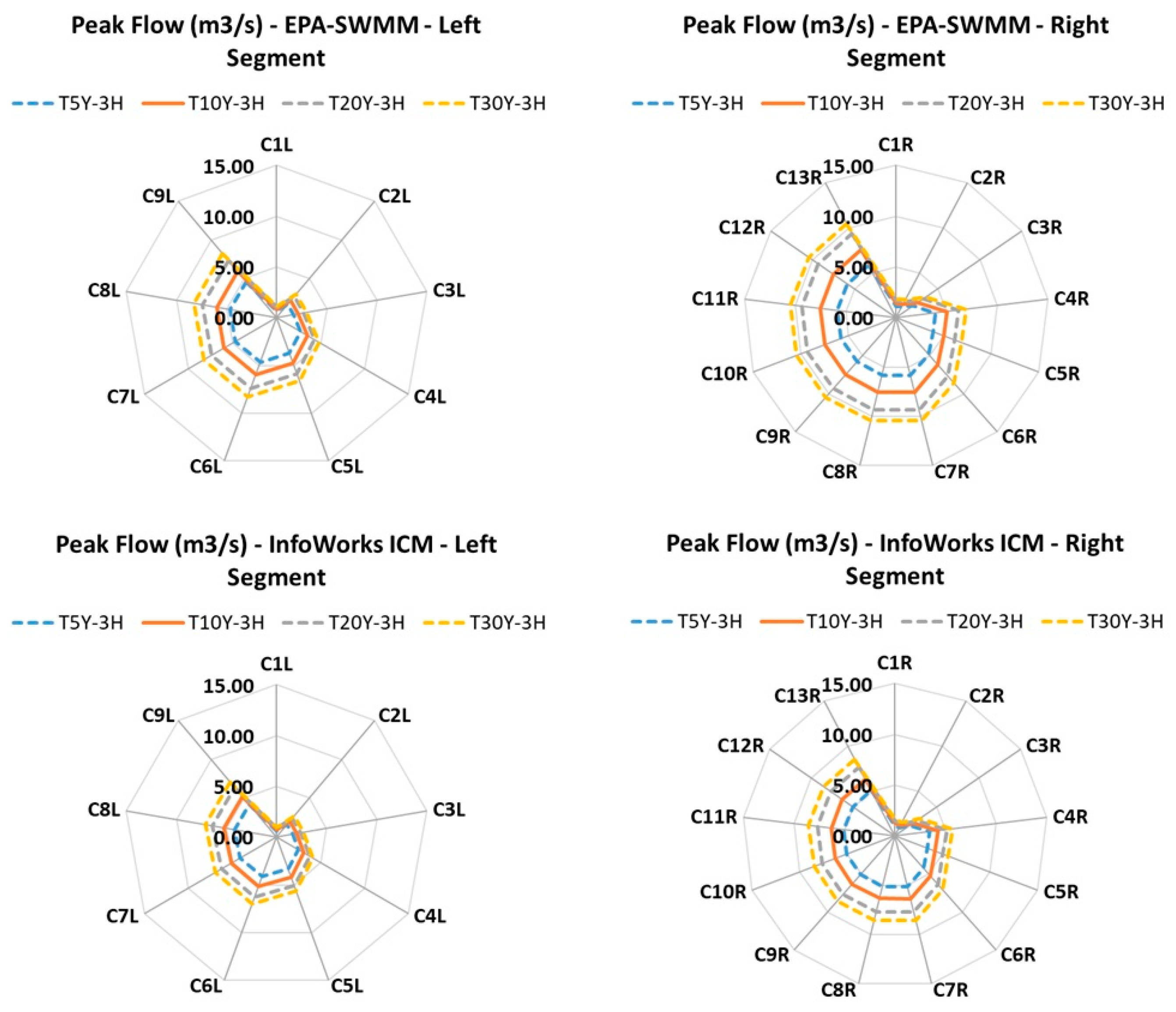
The pipe profiles’ visual comparison was done using radial graphs representing each conduit to display the values of peak flow and relative depth (max depth/diameter) at peak flow. The max depth and speed maps were compared against each other, inspecting any perceivable and significant change to the eye. The runoff quantity continuity was obtained from the status report of each EPA-SWMM 5.2 Simulation.

2.5. Rainfall Input

Most studies of floods in urban areas focus on short-duration, unimodal rain events [28] (p. 3). Generally, two- or three-parameter depth–duration–frequency (DDF) curves are estimated in hydrology studies to derive storms of fixed duration and return period for hydraulic infrastructure design and risk assessment. In urban areas, the contribution of short rainfall events is fundamental due to the fast response of the catchment.
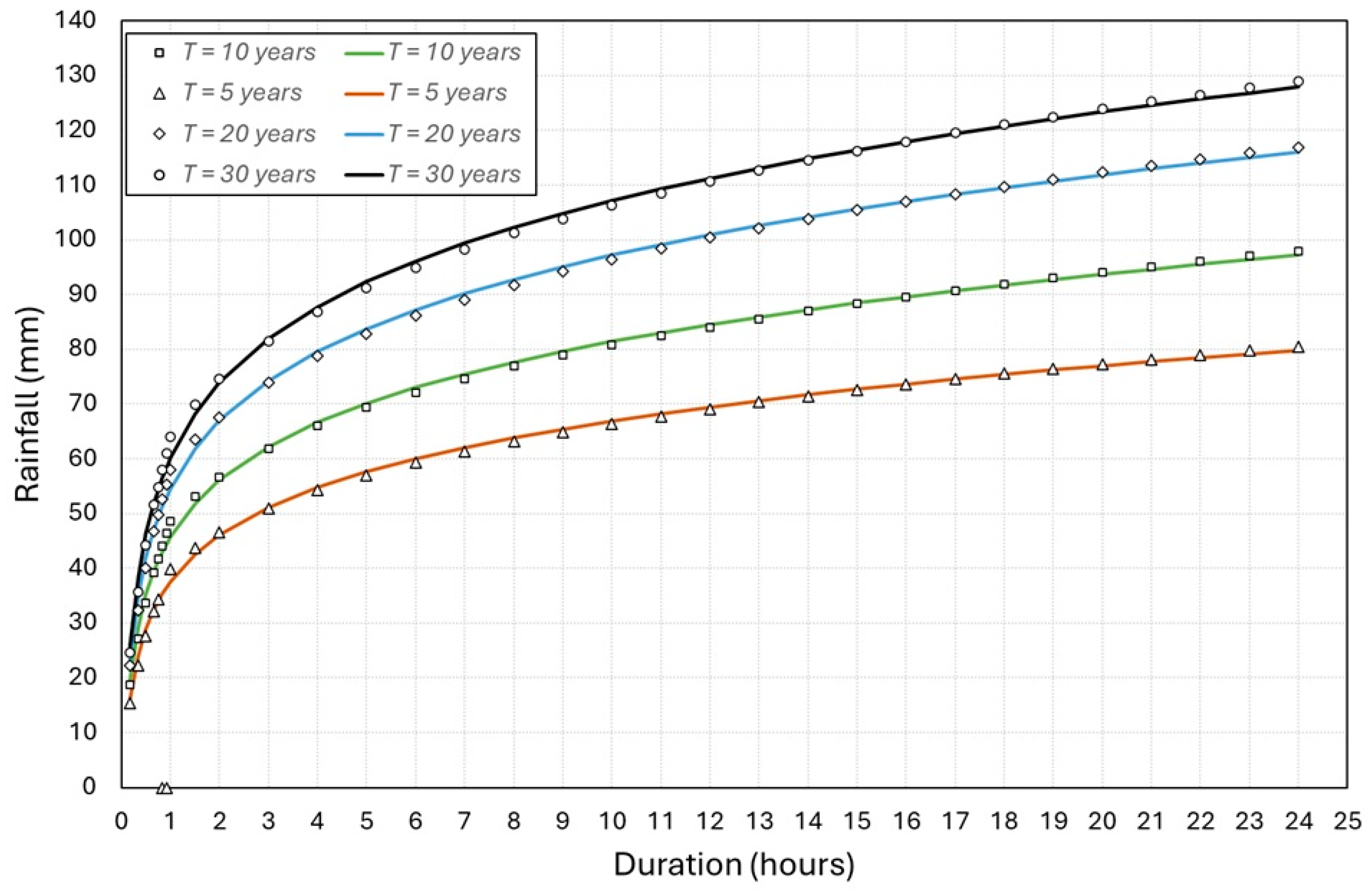
For this study, a three-parameter DDF curve was constructed. For each return time, the quantiles for different durations of rainfall have been first derived by applying the regional procedure proposed for the Sicily region, which takes advantage of sub-hourly resolution rain gauges with short functioning periods and low spatial density, and from hourly resolution rain gauges with longer data samples and high spatial density [29].
The generalized extreme value (GEV) scaling model distribution was adopted to derive the quantiles with different hourly durations. The data input for the GEV scaling model distribution consists of forty-nine years of annual maximum rainfall for fixed durations available during the period 1953–2006 from the Ganzirri rain gauge station, located within the study area and operated by the Water Observatory of Sicily Region (WOS), formerly the Sicilian Regional Hydrographic Service [30]. Sub-hourly rainfall quantiles have been derived using the regional parameters proposed in [29] for the northeast subregion.
For each selected return period, the three-parameter DDF curves have been obtained by fitting the derived quantiles with relationships expressing rainfall depth (h) as a function of duration (d) for each return period considered, as follows:
h d = a · d ( b + d ) c
In Equation (1), the parameters a, b, and c have been estimated through an optimization process based on the least squares method (refer to Appendix A.1 for the values of the parameters), resulting in the curves shown in Figure 5.
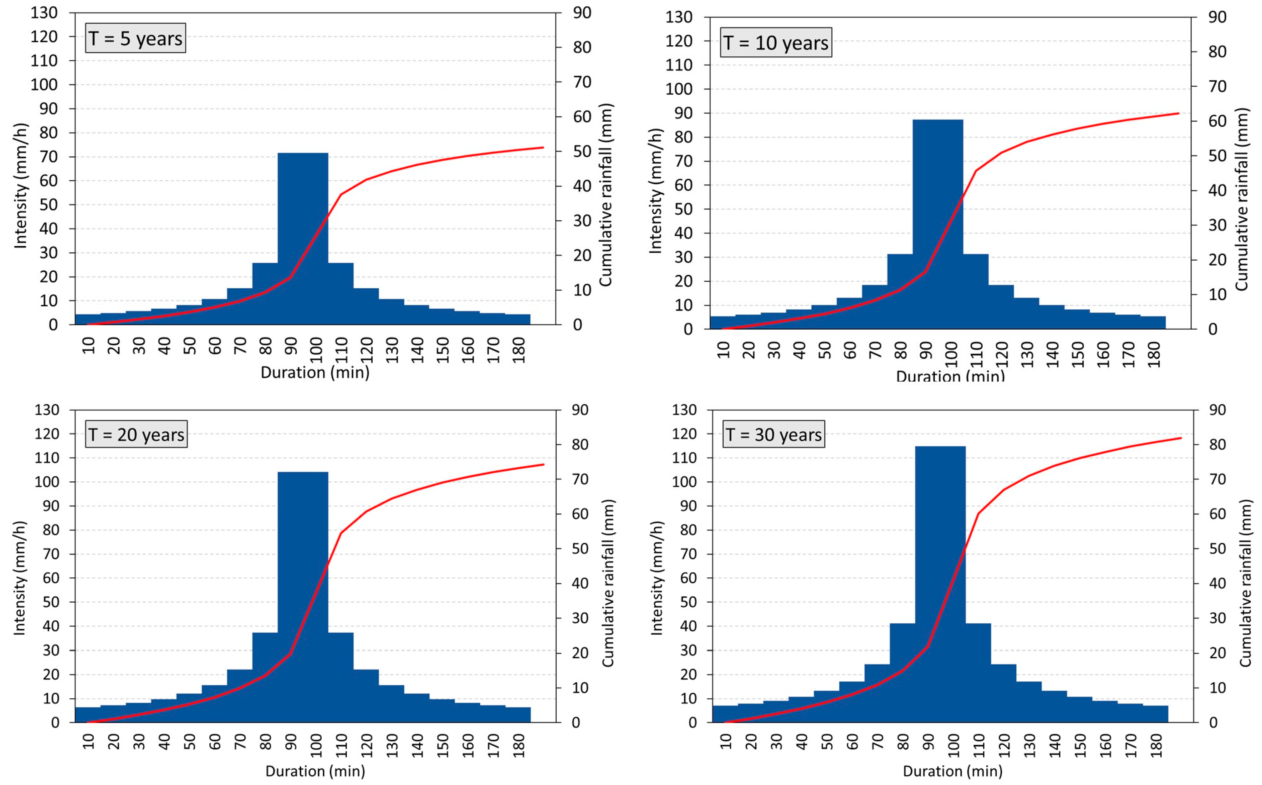
With the DDF curves, the Chicago hyetograph method was used to compute 3 h duration unimodal design rainfall for 5, 10, 20, and 30-year return periods (Figure 6). This method was employed due to its low requirements for basic data and effortless simulation of rainfall intensity [31] (p. 951).
Refer to Appendix A.2 for the rainfall intensities applied in this study.

2.6. Terrain and Land Cover Data

Generally, a hydrodynamic simulation requires basic data about the presence of roads, buildings, permeable and impermeable areas, topography, node distribution, and land and soil cover. The case study of Lake Ganzirri does not have a functional pluvial drainage system, as the runoff was free to flow toward the lake before Directive 2000/60/EC came into place. Table 3 describes the data provided for this study.
The building’s footprint data was obtained from OpenStreetMap and accessed in August 2024. The roads’ polygon shapefile was manually digitized using aerial photos.

2.7. Data Preparation

The spatial data provided for this study were organized in shapefiles, allowing easy importation as features in both HEC-RAS 6.2 and InfoWorks. Table 4 details how to manage every feature and how it was used in HEC-RAS 6.2 and InfoWorks ICM 2021.9.
The perimeter of the study area was traced as a “donut-shaped” (refer to Figure 4) to exclude the lake and reduce the number of mesh elements. This is feasible as the lake is part of a system connected to the sea, and any flow entering the lake does not significantly change the water level enough to cause overflow to populated areas.
Using the donut-shaped perimeter to delimit the 2D zone produces a small gap of 0.16 Ha on the south side of the lake, which was not covered by the mesh. However, this is a small area compared to the total perimeter area, which is 154.91 Ha, and does not significantly compromise the calculations.
The urban sub-catchments were delimited according to [22] (pp. 105–114). The sub-catchments cover the areas draining towards Via Consolare Pompea (refer to Figure 4) and were used to design the drainage system and the SUDS strategies. The hydrological features required for the EPA-SWMM 5.2 model and InfoWorks ICM 2021.9 were computed and are detailed in Appendix A.3.

2.8. Representation of Topography and 2D Domain

The raster file provided (ASC File) was clipped using the perimeter of the case study and GIS tools. Then, the clipped file was imported into HEC-RAS 6.2 and InfoWorks ICM 2021.9 to create the RAS terrain and the ground model grid, respectively. Both elements represent the topography of the study area. The rounding (precision) for the RAS terrain was set to 1/128, and the base cell size (XY) for the ground model grid was left at the minimum resolution of the ASC file raster, which is 2 m.
To define the 2D domain (meshing area). The 2D flow area (HEC-RAS 6.2) and 2D zone (InfoWorks ICM 2021.9) were defined by importing the shapefile describing the perimeter of the study area. They were given a Manning’s roughness coefficient of 0.011 (concrete coverage considered by default) with a mesh element size of 10 × 10 m for HEC-RAS 6.2 and a maximum area of 100 m2 for InfoWorks ICM 2021.9. A minimum element area of 4 m2, mesh generation by “clip meshing”, normal condition for the boundary points, the option “apply rainfall directly to mesh elements” checked, and apply rainfall outside of the sub-catchment. The latter is to avoid double-counting the rainfall when applying the lumped approach. These features will be adjusted with the presence of buildings, roads, and permeable areas, where infiltration, roughness, mesh refinement, and topography modifications were implemented to represent the urban features.

2.9. Representation of Buildings, Roads and Permeable Areas

The application of hydrological and hydraulic models in risk assessment and flood forecasting has sparked attention in recent years, as there is a need to develop more accurate representations of reality with effective simulation times for flood maps, nowcasting, and disaster risk management purposes [32] (p. 3). Moreover, the location of urban green spaces, the layout of roads, the shape of the buildings, and their spatial distribution (building density) directly influence urban flood behavior [33] (pp. 2, 8–13). Regarding the representation of buildings, the typical modeling strategies are as follows [34] (p. 3), [35] (p. 1605), [36] (p. 8):
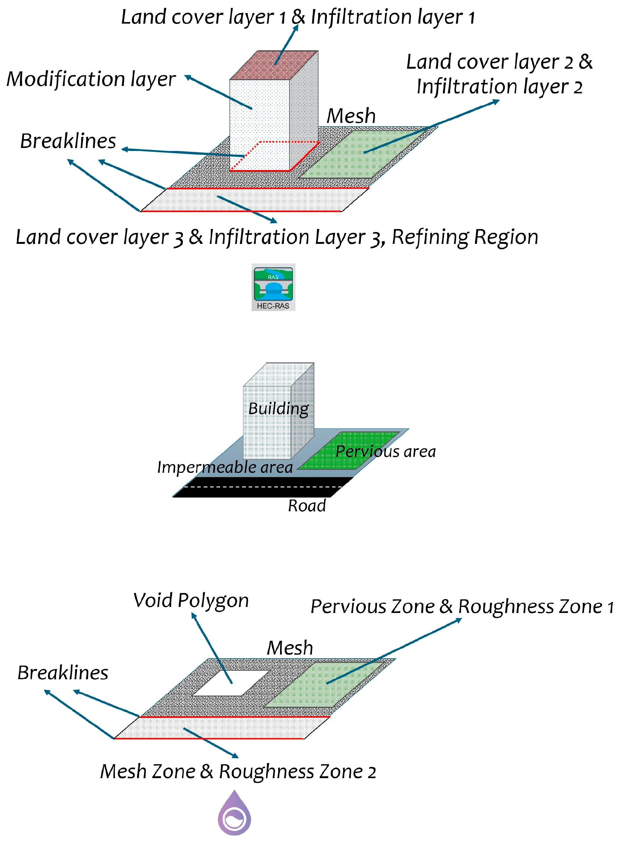
  • Building void (BV): Consider buildings as voids in the mesh. These areas are not taken into account for the analysis and computations;
  • Building with solid walls (BSW): Imposed solid wall conditions on the boundaries of each building;
  • Building resistance method (BR): A parameter is set at high values to keep the runoff flowing “through” the buildings (e.g., infiltration rate);
  • Building block method (BB): Involves adding artificial elevations to the topography of the buildings’ footprints.
InfoWorks ICM 2021.9 can apply BV directly by importing the buildings’ shape file as “Void Polygons”. These polygons are not considered for the meshing process. Therefore, InfoWorks ICM 2021.9 manages a concept named the effective area for the calculations, which is the total area of the 2D zone minus the area covered by the void polygons.
HEC-RAS 6.2 does not have a specific tool for BV. Therefore, BSW, BR, and BB were applied simultaneously (Figure 7).
BSW was applied by extracting the polygon boundaries of the buildings’ shapefile using GIS tools and importing them as break lines to keep the mesh free of cells on top of two or more land covers (Figure 7). BR was implemented by importing the buildings’ shapefile as an infiltration layer created with the deficit and constant loss method (Def-Con), which represents the soil as a single layer that gains or loses moisture depending on its characteristics. BB was applied using the modification layer tool (add modification → polygons → multipoint), setting the elevation type to “AddValue” and a four-meter fixed elevation value.
The permeable areas require roughness and infiltration features to represent their effect on the urban domain. The polygons were imported into HEC-RAS 6.2 as land cover and infiltration layers. To define the roads, roughness, smaller mesh cells, break lines, and some modifications to the RAS terrain are required. As in the permeable areas, the polygon shapefiles were imported into HEC-RAS 6.2 as land cover and infiltration layers. Details of the parameters used for constructing the HEC-RAS 6.2 and InfoWorks ICM 2021.9 2D models are detailed in Appendix C.2.

2.10. Meshing Details and Adjustments for Representing Flow Around Buildings in HEC-RAS 6.2

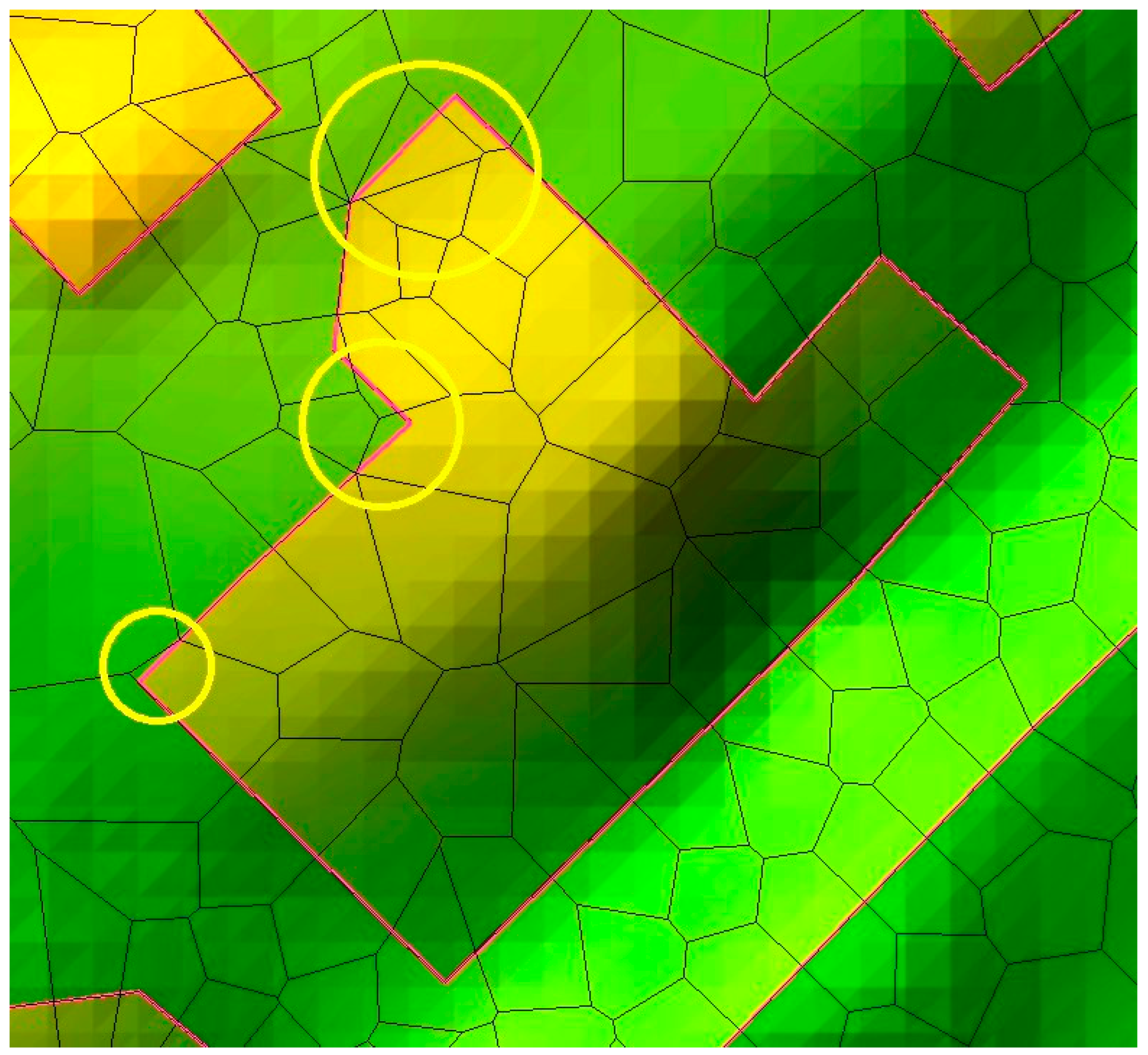
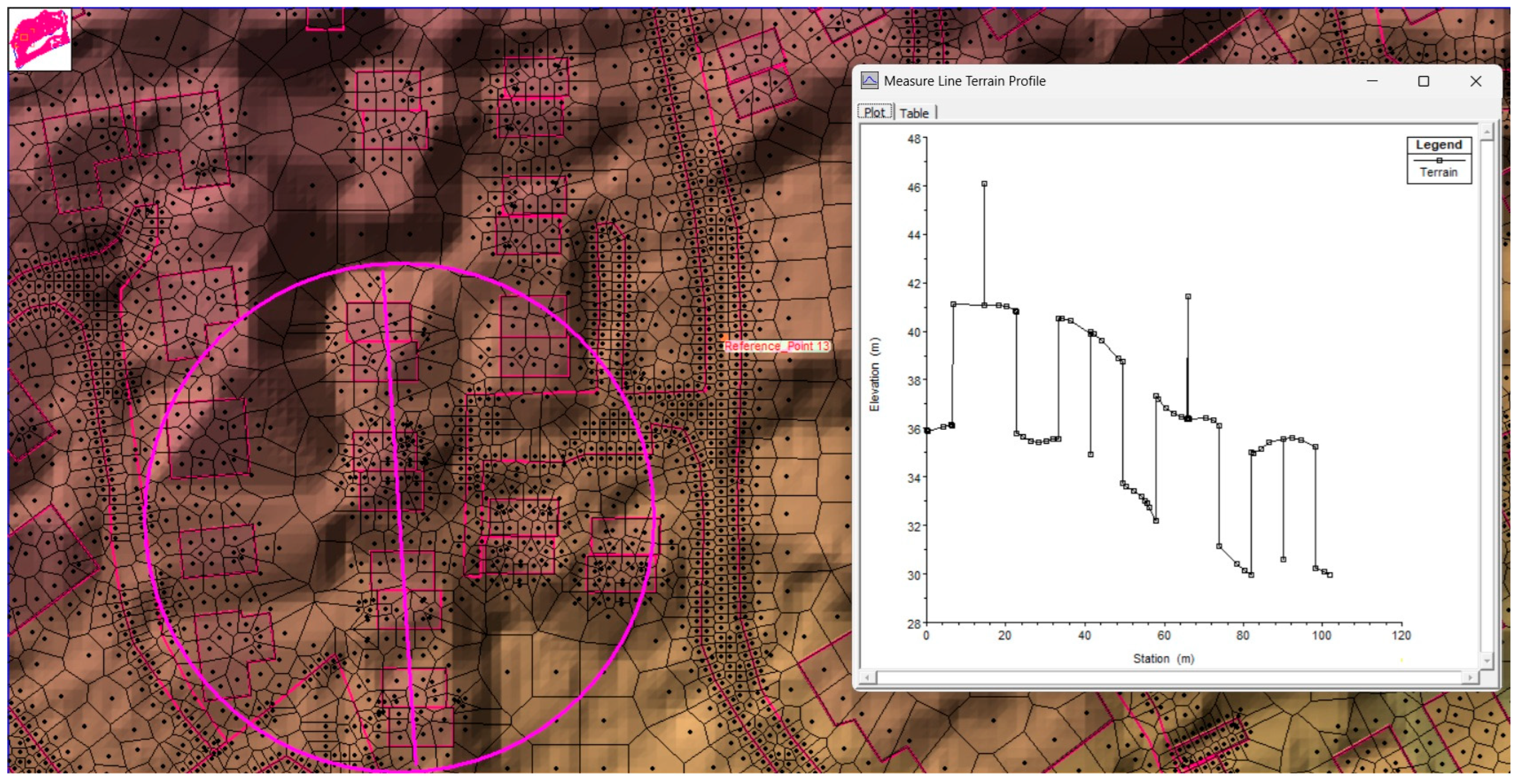
For HEC-RAS 6.2, the mesh’s grid size was 10 × 10 m (Cell Size X = Cell Size Y = 10), with local refinements from 2 m to 5 m around buildings to represent details in the topography, roads, and building presence. This was done by reinforcing each breakline around buildings after generating the mesh. Generally, the corners of buildings, especially the ones with complex shapes, resulted in cells partially covering the building’s footprint and another land cover type (Figure 8). If this were the case, the breakline cell spacing was reduced to 5 m (both minimum and maximum blank for mesh spacing) and reinforced again. The process was done until no cells partially covered a building’s footprint and another land cover, requiring reductions of cell spacing down to 2 m in some cases, and even moving some calculation points on the mesh.
Figure 8 illustrates the central issue when representing buildings using HEC-RAS 6.2. The irregular shape of some buildings and the presence of many vertices describing the sides of the polygons (e.g., a straight side of a building defined by three or more vertices) influenced the meshing process, resulting in cells covering buildings’ footprints and other land cover despite the use of break lines. This issue was generally present in sharp edges and corners, and fixing included break line reinforcing on each building perimeter and refining the break line cell spacing to fit whole grid elements inside the building’s footprint, requiring manual inspection of each building and time-consuming manual refinements. Consequently, the number of mesh elements increased from 58,422 (after the first mesh generation) to 64,787 elements after all the refinements in the buildings.
In contrast, for the meshing process in InfoWorks ICM 2021.9, the 2D zone was configured to have a maximum triangle area of 100 m2, a minimum element area of 4 m2, the mesh generation method is “clip meshing”, the boundary points were set to “normal condition”, the minimum angle of the triangles forming a mesh was set to 25 degrees, a Manning coefficient of 0.011, with the options of “apply rainfall etc directly to mesh elements” and “apply rainfall etc.” checked. Both meshing process characteristics have been used in models with similar characteristics of urbanization [19,20].

2.11. Pluvial Drainage System Design

The software EPA-SWMM 5.2 was used to design a pluvial drainage system for the 3 h duration and a 10-year return period total rainfall event (T10Y-3H; see Appendix A.1). The proposed network aims to drain the runoff that requires capture and conveyance away from Via Consolare Pompea to avoid water flowing into the lake.
All the sub-catchments were traced upon a backdrop georeferenced image. The area, width, and slope were calculated using spreadsheets and GIS Tools.
The infiltration process was modeled using the SCS curve number (CN) method, which allows for the computation of the hydrological loss due to permeable areas in a catchment. The following equations describe the method [37] (p. 82):
Q = ( P I a ) 2 P + S m a x I a
S m a x = 254 100 C N 1
Q represents the total runoff and P the total volume of rainfall (both expressed in mm) of the considered event. I a represents the initial abstraction (mm), Smax is the soil moisture storage capacity (mm), and CN is the curve number that depends on the land cover type and is tabulated. EPA-SWMM 5.2 requires some adjustments to approximate the curve number method in a catchment [37] (p. 82): setting the percentage of impervious area of the sub-catchment equal to zero, selecting the curve number, setting the pervious depression storage equal to the initial abstraction depth that one would otherwise use with the SCS method, and setting the permeable area roughness coefficient to zero. However, instead of selecting the curve number from tables, it was calculated using an indirect method based on the mean runoff coefficient ( φ ), which is based on the proportion of the catchment’s permeable and impermeable areas [38] (p. 225):
φ = φ p e r m · 1 A i m p + φ i m p · A i m p
where φ p e r m and φ i m p are exit coefficients for pervious and impervious areas, which were set to 0.3 and 0.9, respectively [39]. The parameter A i m p represents the percentage of impervious area in the catchment. The indirect method defines the initial abstraction equal to zero for urban areas ( I a = 0 ), and the mean runoff coefficient is also equal to the relationship between the total runoff and the total precipitation, resulting in:
Q = P 2 P + S m a x
φ = Q P
Combining Equations (4) and (5) and solving for Smax results in:
S m a x = P ( 1 φ ) φ
Equation (2) can be modified to express CN in terms of Smax:
C N = 25,400 254 + S m a x
Equations (4), (7), and (8) were used to calculate the curve number for each sub-catchment, and the parameter “d-store perv” was calculated as 0.2 times Smax following the manual’s recommendations. The calculated values are listed in Appendix A.4.
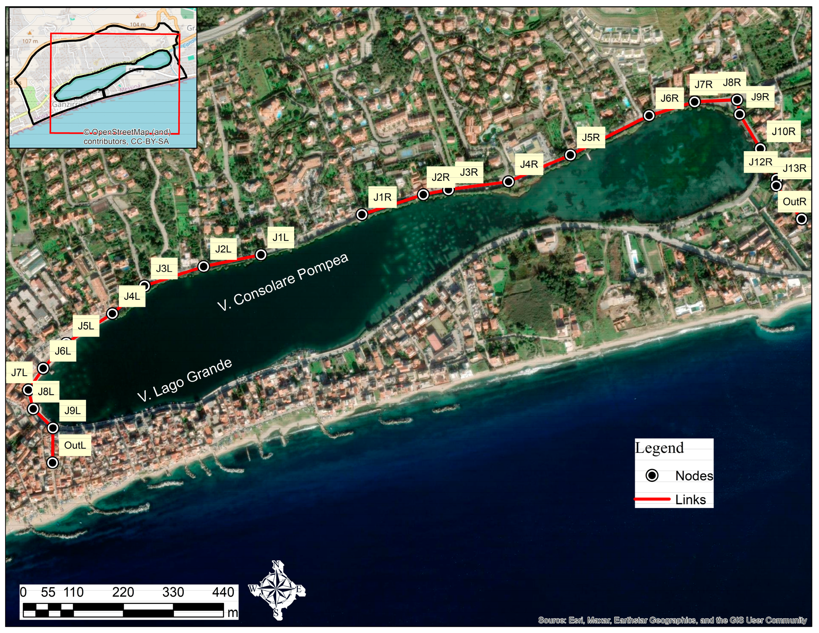
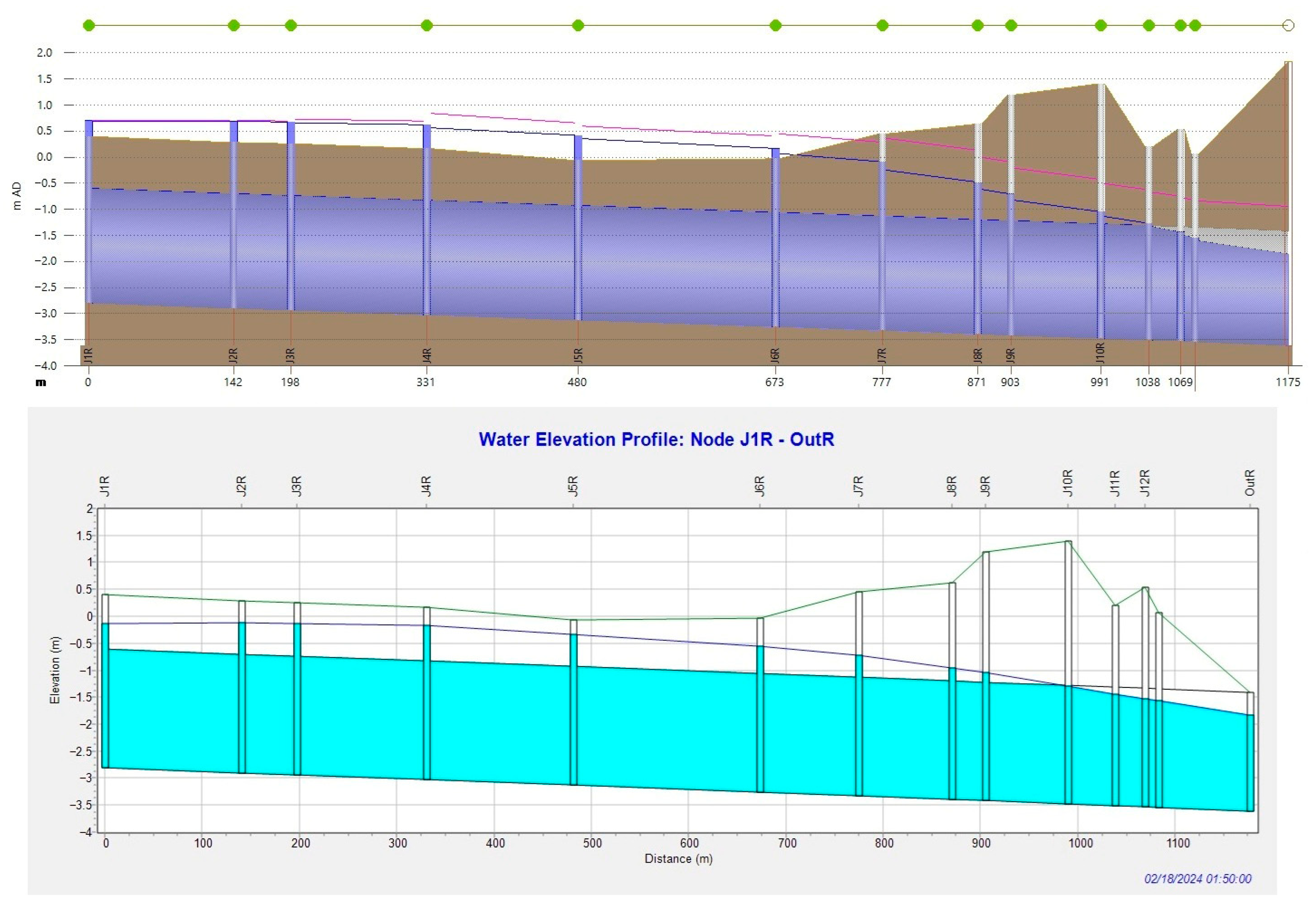
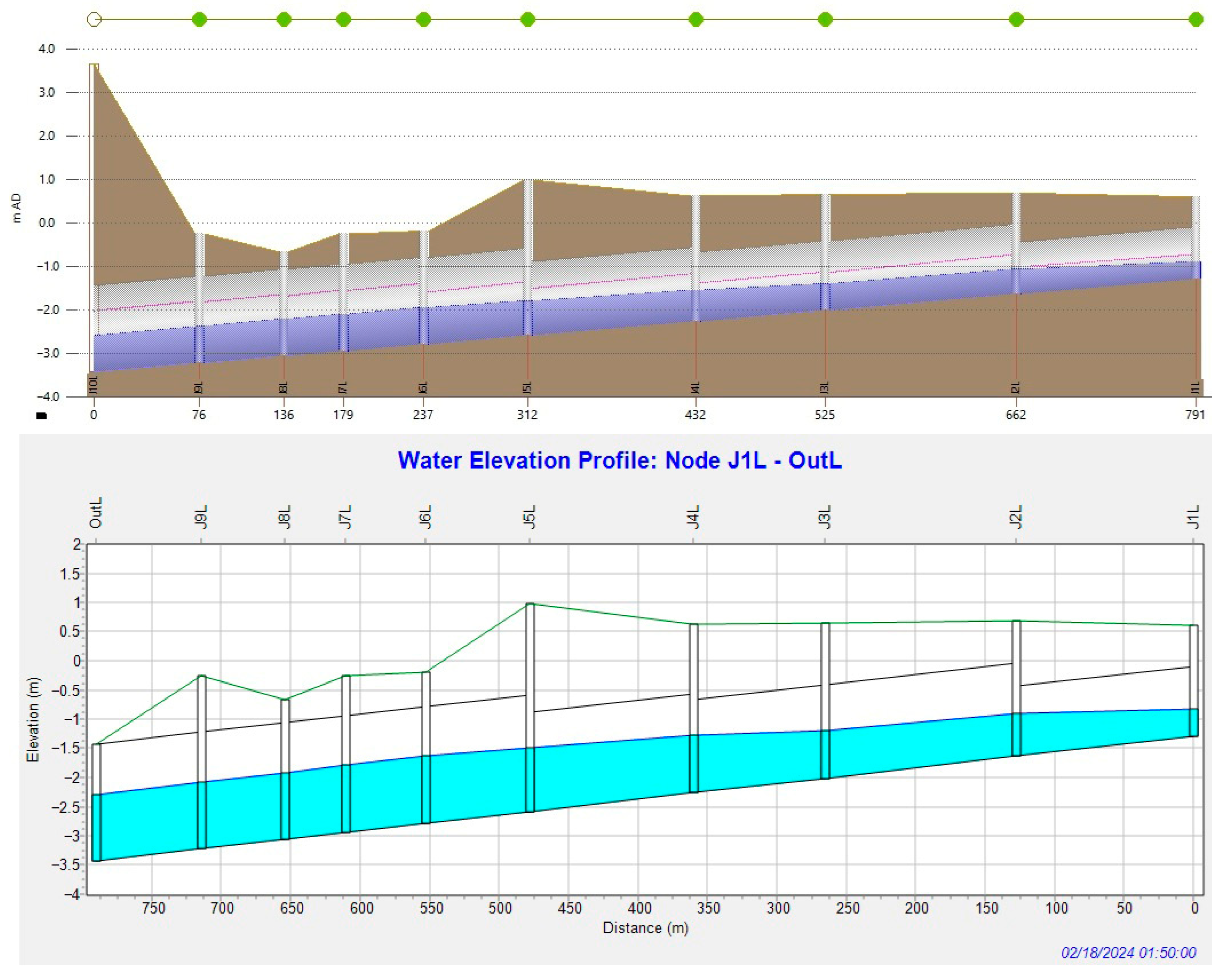
The design considered two segments (left and right) discharging into key locations to project reservoir tanks to be pumped somewhere else with nodes on Via Consolare Pompea that connect with other nodes under Via Lago Grande, Via Michelangelo Vizzini (in the left segment) and Via Canaloni connecting with small passages between houses in the area (in the right segment) (Figure 9).
The design was limited to the drainage until the outlets, which are assumed to be connected to reservoirs where water will be pumped out of the study area. Therefore, the design does not include pumping and conveying outside the study area.
The design considered circular PVC conduits (Manning N = 0.009) connecting the nodes (see Appendix B for more details). The design parameters were that all pipes should have a relative depth at peak flow (max/full depth in EPA-SWMM 5.2) less than 0.9 and speeds not exceeding 6 m/s. The diameters of the left segments range from 1.2 to 2 m, and all the pipes of the right segment have a diameter of 2.2 m. The topographic conditions of the surroundings of Lake Ganzirri are complicated, requiring extensive excavations to make room for the pipe system to comply with the design parameters. Therefore, both outlet discharges are at −3.43 and −3.61 m below sea level, with very low slopes of 0.2710% and 0.0683% for the left and right segments, respectively.

2.12. Simulation Parameters for 2D Approach and Sub-Catchment Properties for 1D Approach

For HEC-RAS 6.2, the reference simulation scenario (S0) involves an unsteady two-dimensional flow routing solved with the Shallow Water Equations–Eulerian–Langrangian method (SWE-ELM) for each rainfall event with a computation interval of 0.1 s. All computation options and tolerances were left at default values, except the advanced time step control, where the option to adjust the time step based on Courant was activated. The settings were adjusted according to Table 5. The mapping output interval, the hydrograph output interval, and the detailed output interval were set at 2 min.
For InfoWorks ICM 2021.9, the tool Scenarios was used to create the simulation scenarios described in Section 2.3. This tool can model network variations by creating an editable copy within the same model group. All simulation parameters were set to default values. A run file was created for each scenario for all rainfall events. The time step was set at 10 s, the results timestep multiplier was set to 6, and a 3 h duration simulation. The 2D parameters were set to default values, and the option to use the graphical processing unit (GPU) for 2D calculations was checked.
Comparisons B, C, and D required the consideration of a sub-catchment delimitation (Figure 4). These cases were managed using EPA-SWMM 5.2 and InfoWorks ICM 2021.9. Both software programs needed the definition of sub-catchment properties to run the models. For EPA-SWMM 5.2, all the sub-catchments were traced upon a backdrop georeferenced image. The area, width, slope, and depression stored for pervious areas were calculated using spreadsheets and GIS tools. The curve number method was set for the infiltration data, and each sub-catchment was assigned the curve number calculated as described in Section 2.11. The drying time was set to 7 days. For InfoWorks ICM 2021.9, four runoff surfaces were defined with the properties described in Appendix C.3. The runoff surfaces were associated with the default land use assigned to each sub-catchment. Each runoff surface area per sub-catchment was calculated using GIS tools and assigned in the sub-catchment properties window.

2.13. LID/SUDS Strategy

Generally, implementing LID/SUDS will alter the proportions of roof area, roads, and permeable and impermeable areas in an urban catchment to drain the runoff using infiltration, retention, and storage devices [40] (p. 1). For instance, permeable pavement will replace impermeable asphalt roads, green roofs will replace concrete or tile roofs, and bioretention systems can replace available green areas. Therefore, a quantification of roof area (buildings), roads, and permeable and impermeable (residual) areas for each sub-catchment was computed (Table 6).
The LID/SUDS Strategy explored reducing runoff volume by combining green roof coverage, permeable pavement implementation, and bio-retention cells. The strategy was represented using the LID Control option in EPA-SWMM 5.2, assigning parameters recommended in the literature [31,41,42] (refer to Appendix C.4).
The strategy explored substantial retrofits, such as combining all roof areas covered in standard green roofs, implementing a permeable area on the roads between Via Panoramica and Via Consolare Pompea, excluding these two, and turning 30% of the available permeable area of each sub-catchment into bioretention cells (Table 7). The percentage did not follow any policy or rule. It was estimated based on the spatial distribution of the available green open spaces to avoid being invasive and leave walkable green spaces for pedestrians.
The 2D representation of LID/SUDS objects was performed only on InfoWorks ICM 2021.9, which does not have specific tools for LID/SUDS objects for a 2D zone. Therefore, 2D LID/SUDS objects can be represented by adjusting the mesh and roughness zones, and infiltration surfaces (2D) and zones to replicate infiltration or retention capabilities. In this study, buildings were represented using the BV approach. Consequently, a limitation was created to represent green roofs, as the BV approach excludes the buildings’ footprint from the meshing. Therefore, the 2D adaptations in this study included only bioretention cells and permeable pavements (Table 8).

3. Results

3.1. Comparison A—Scenario S0 in InfoWorks ICM 2021.9 and HEC-RAS 6.2

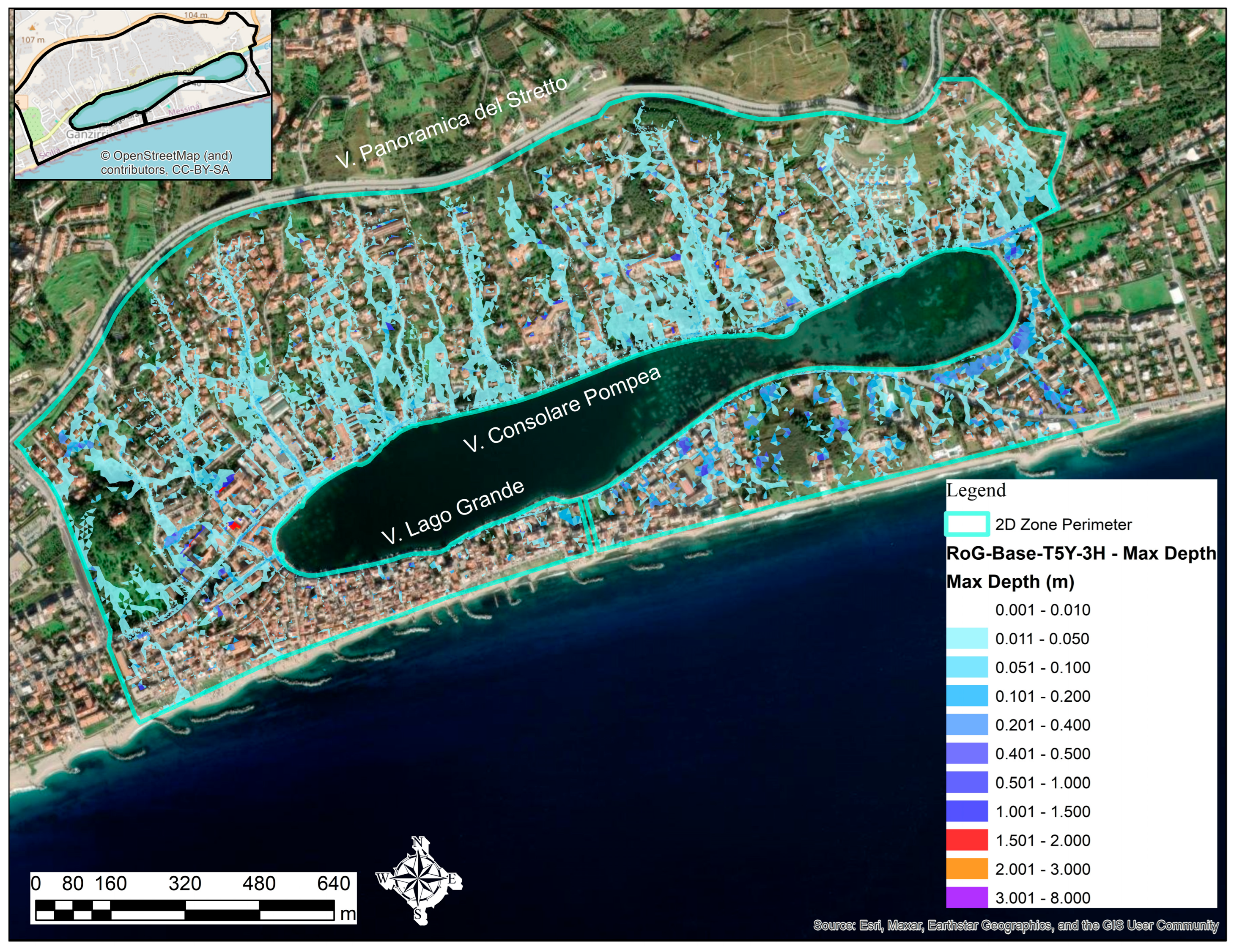
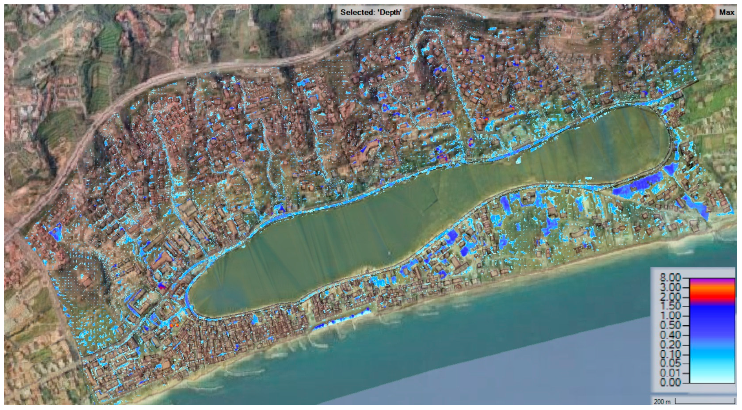
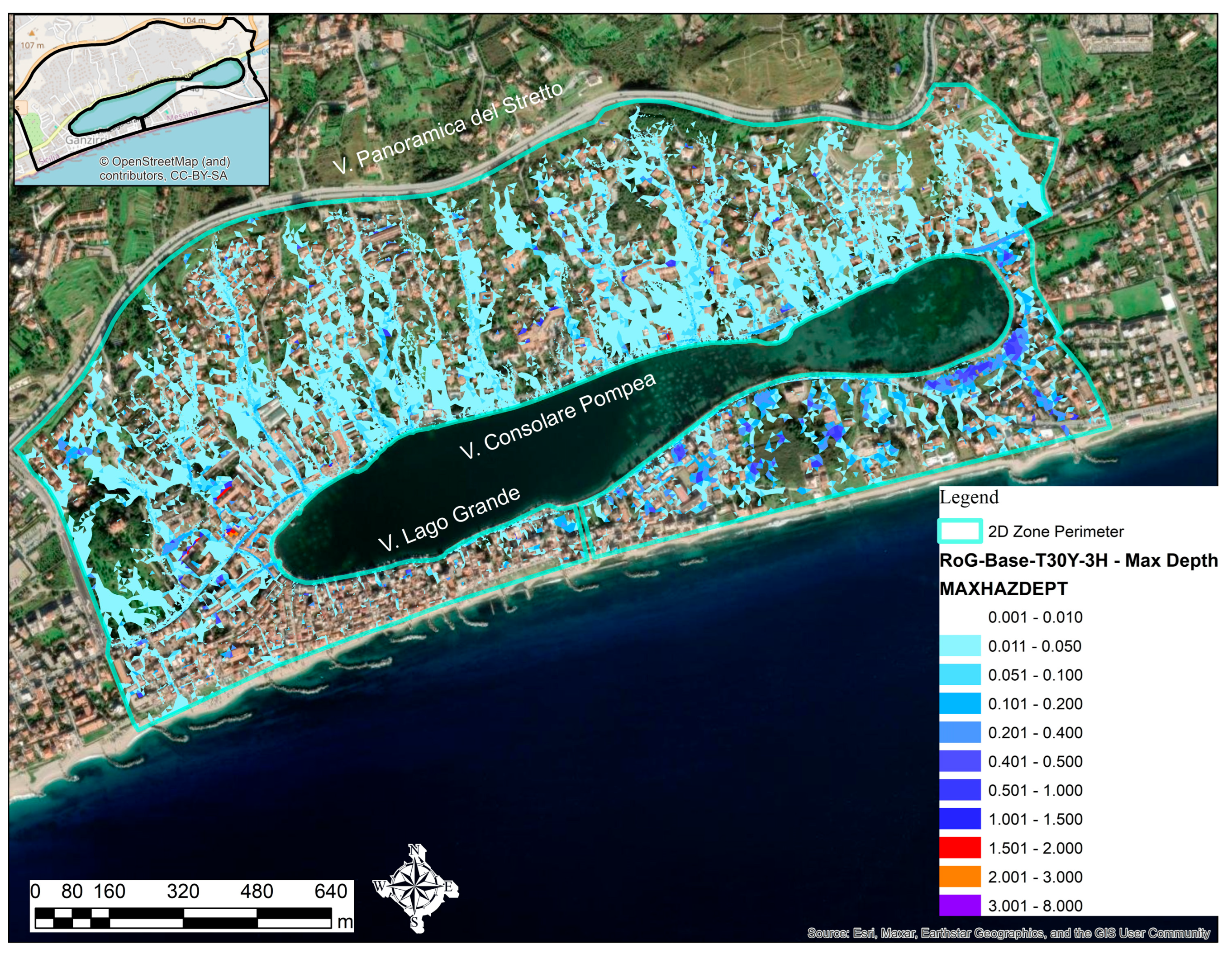
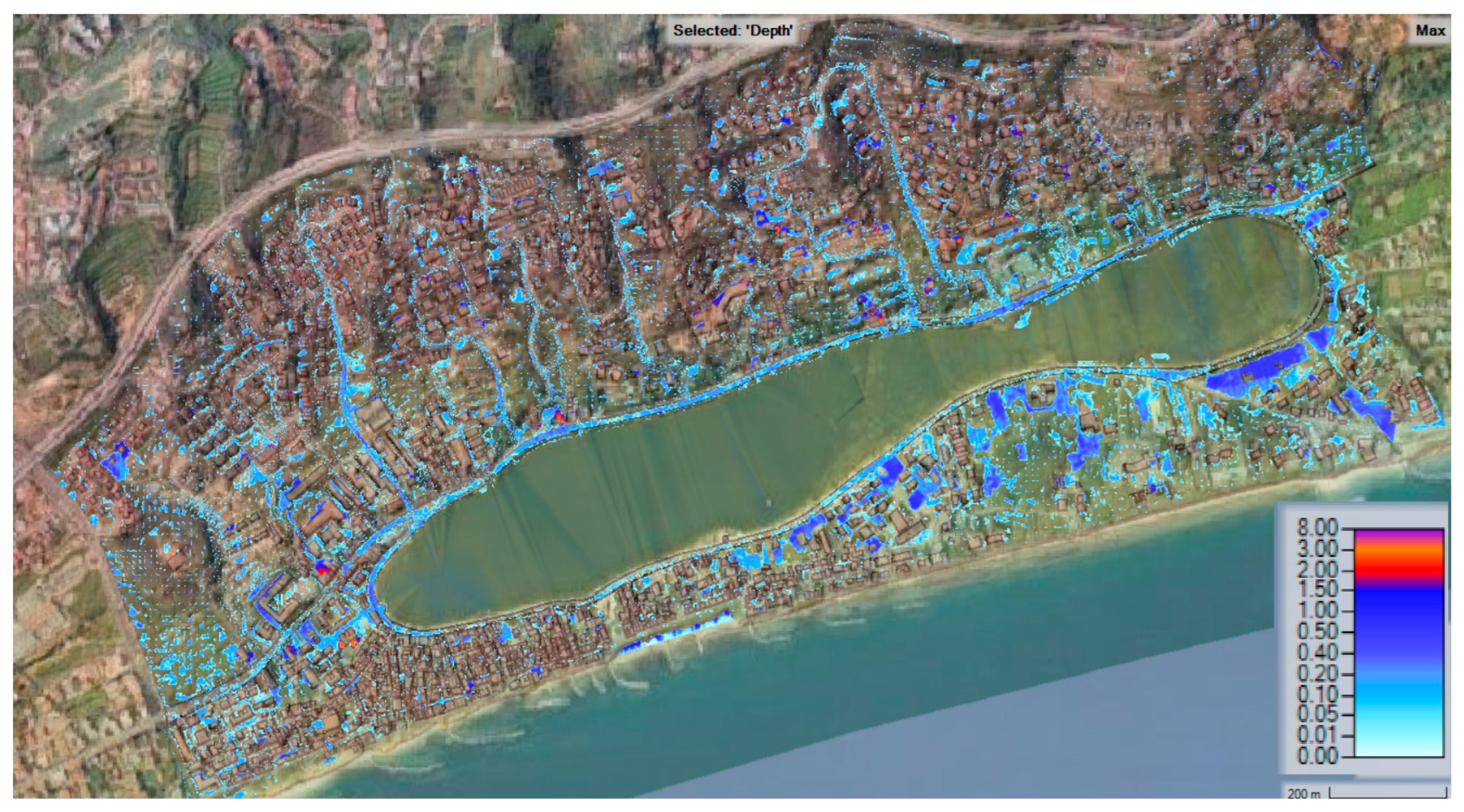
Both models could similarly represent the propagation of runoff over the 2D domain for Scenario S0. The flow propagation moves around the buildings within the 2D domain using the representation methods in the literature. When exploring the statistics of the 2D simulation in both software programs (Table 9), the maximum value of “max depth” on the mesh calculations is substantially different.
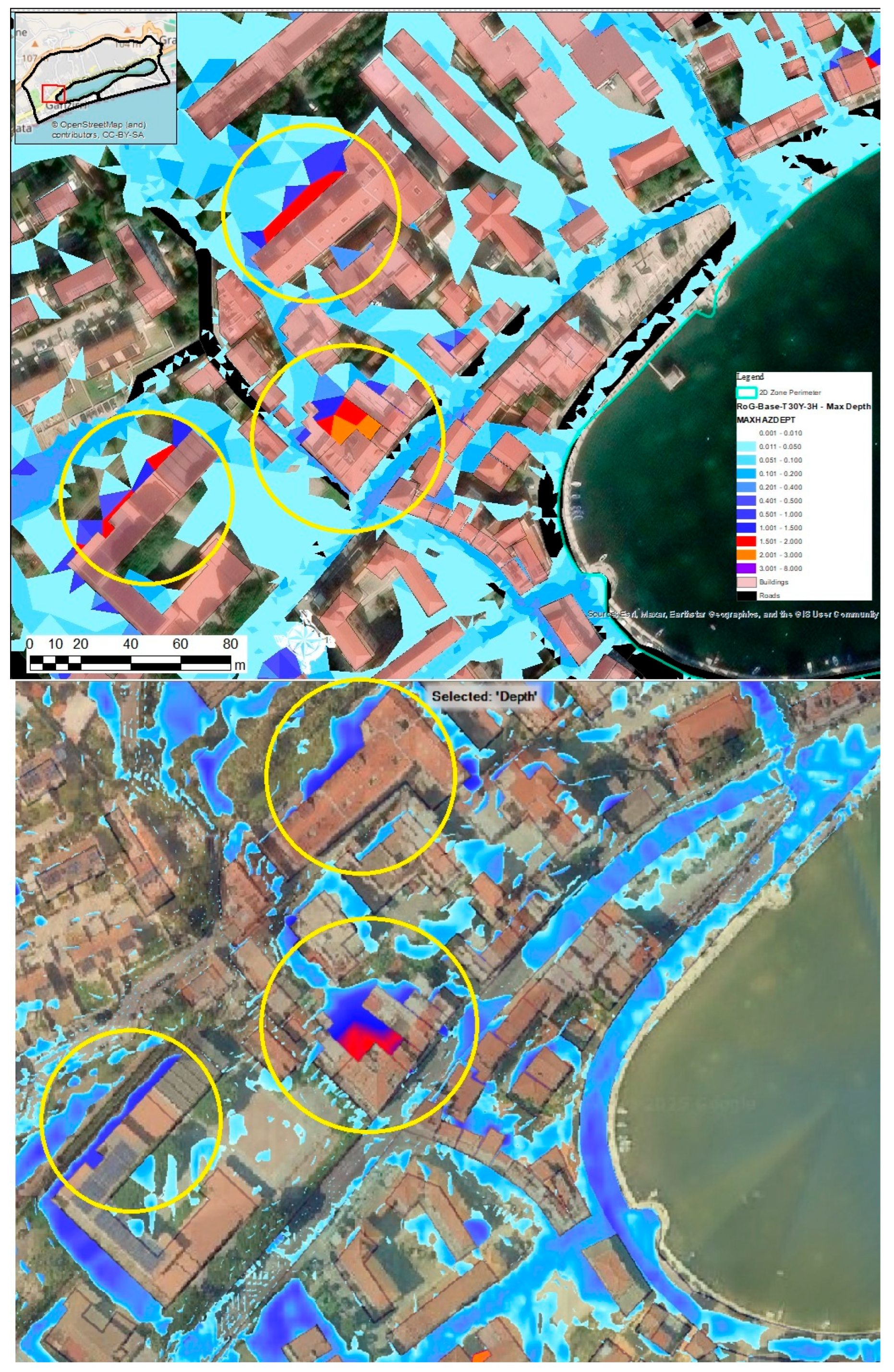
For the sake of brevity, Figure 10, Figure 11, Figure 12 and Figure 13 present only the maps for rainfall events with return periods of 5 and 30 years. Both sets display the propagation in reasonable agreement with each other in a broader sense, especially over Via Consolare Pompea. The legend marks water depths above 1.5 m on a different palette for further analysis, as they are initially considered unrealistic. These unusual water depths were present in both models.
Table 10 presents the mean absolute error (MAE) of the maximum depth and maximum speed extracted from the reference points across the 2D domain (refer to Figure 4), which increases with increasing rainfall intensity.
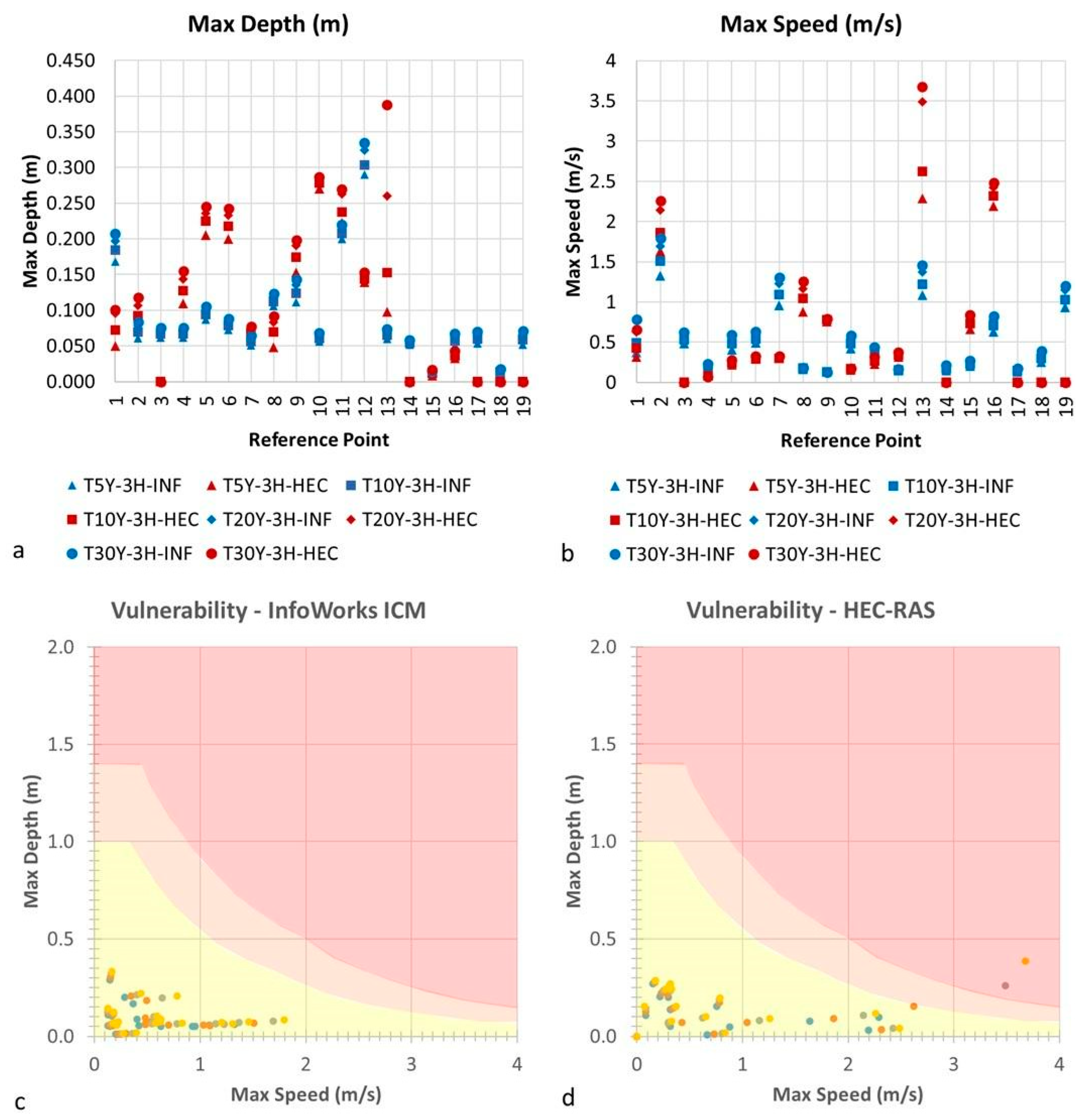
The MAE values range from 6.4 to 8.9 cm, and the max speed from 0.446 to 0.625 m/s. All reference points were set on roads to explore the models’ performance at street level, except reference point no. 17, which is directly located in a vegetated area (highly dense vegetation around a walled perimeter). The reference points with the least absolute error for depth were no. 2, 7, 8, 11, 15, 16, 18, and for maximum speed, no. 1, 2, 4, 11, 12, 14, 17 (Figure 14a,b).
To further reflect on the implications of the obtained differences, we can see the results under the scope of risk analysis as a function of hazard and vulnerability. Regarding hazard analysis, the 2D models on both software programs are enough to reproduce the extent of the pluvial flooding. However, under the frame of a vulnerability analysis, the differences displayed in Figure 14a,b can have significant effects. Figure 14c,d display the maximum depth and speed values of each reference point, for all rainfall events, forming a cloud of points plotted on people’s vulnerability to flood thresholds proposed by [43] (p. 189). In the benchmark (InfoWorks ICM 2021.9 model), all the reference points’ responses to all rainfall events fall in the low vulnerability to floods for people. In HEC-RAS 6.2, the distribution of the results also concentrates on the low vulnerability zone, but reference points 2, 13, and 16 shifted towards larger velocities. Exploring these points further, reference point 2 is located on an open and wide section of Via Consolare Pompea; therefore, HEC-RAS 6.2 produced an unconstrained Cartesian grid in this region, different from the finer unconstrained Delaunay mesh that InfoWorks ICM 2021.9 produced. Points 13 and 16 share similar characteristics with each other. Both are located on a straight section of a road with a steep vegetated area on one side and a flat surface on the other. The difference between models is the mesh type. For HEC-RAS 6.2, a constrained Cartesian grid was calculated for both points compared to the constrained Delaunay grid in InfoWorks ICM 2021.9.
This fact deserves further research, as previous studies have highlighted.
The inundated area ranges from 28% for the rainfall event T5Y-3H, 31% for T10Y-3H, 34% for T20Y-3H, and 36% for T30Y-3H.

3.2. Comparison B—Scenario S1 in InfoWorks ICM 2021.9 and EPA-SWMM 5.2

This comparison scheme focuses on the simulation scenario S1, which explores the 1D representation of urban catchments in a section of the case study area. InfoWorks ICM 2021.9 and EPA-SWMM 5.2 require a sub-catchment delimitation and a pluvial drainage network to use the 1D approach for the hydrological calculations (lumped approach). As explained in Section 2.11, EPA-SWMM 5.2 was used to design the pluvial drainage network, and the same system was replicated in InfoWorks ICM 2021.9 for comparison purposes. Therefore, in this comparison scheme, EPA-SWMM 5.2 is the benchmark.
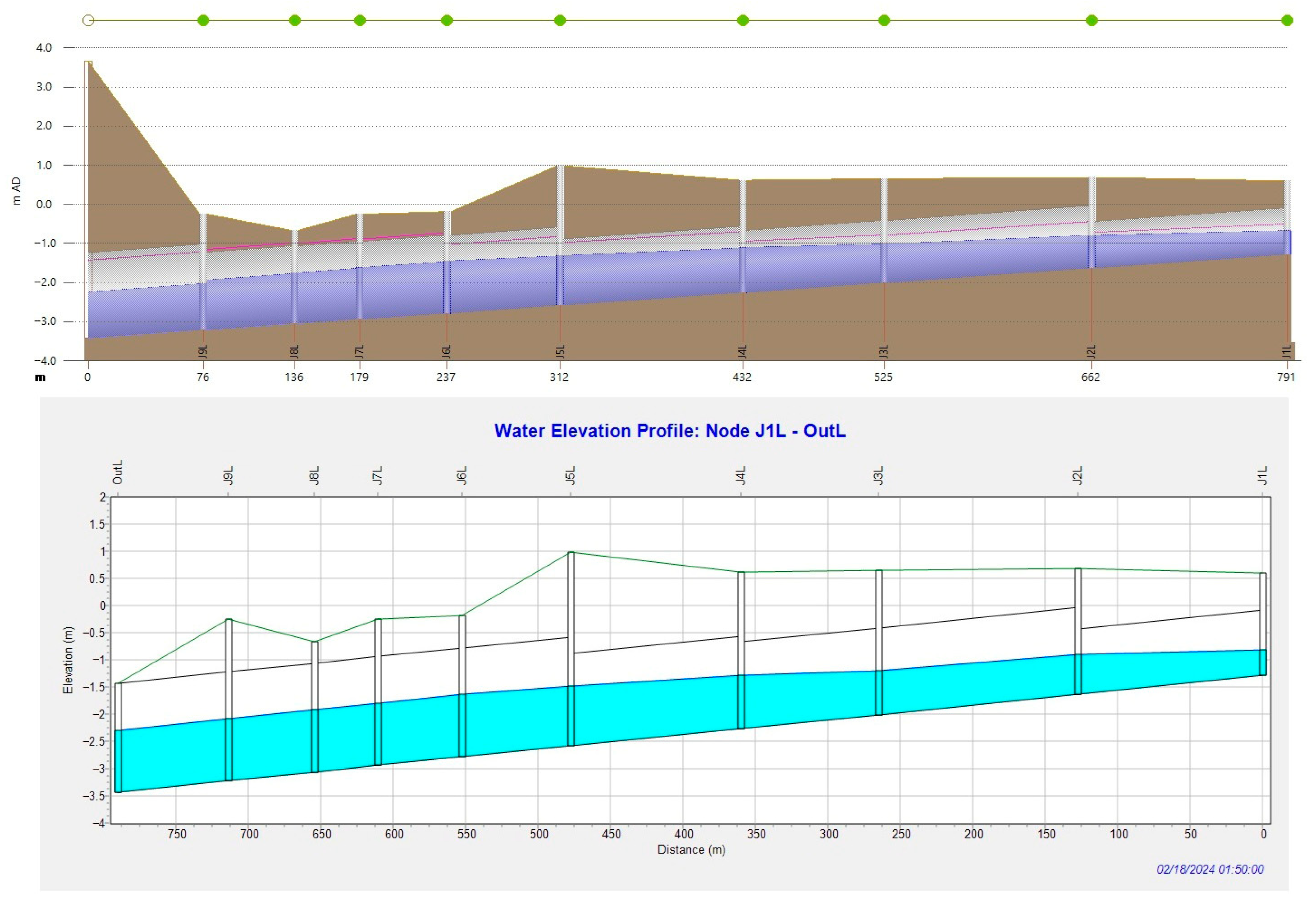
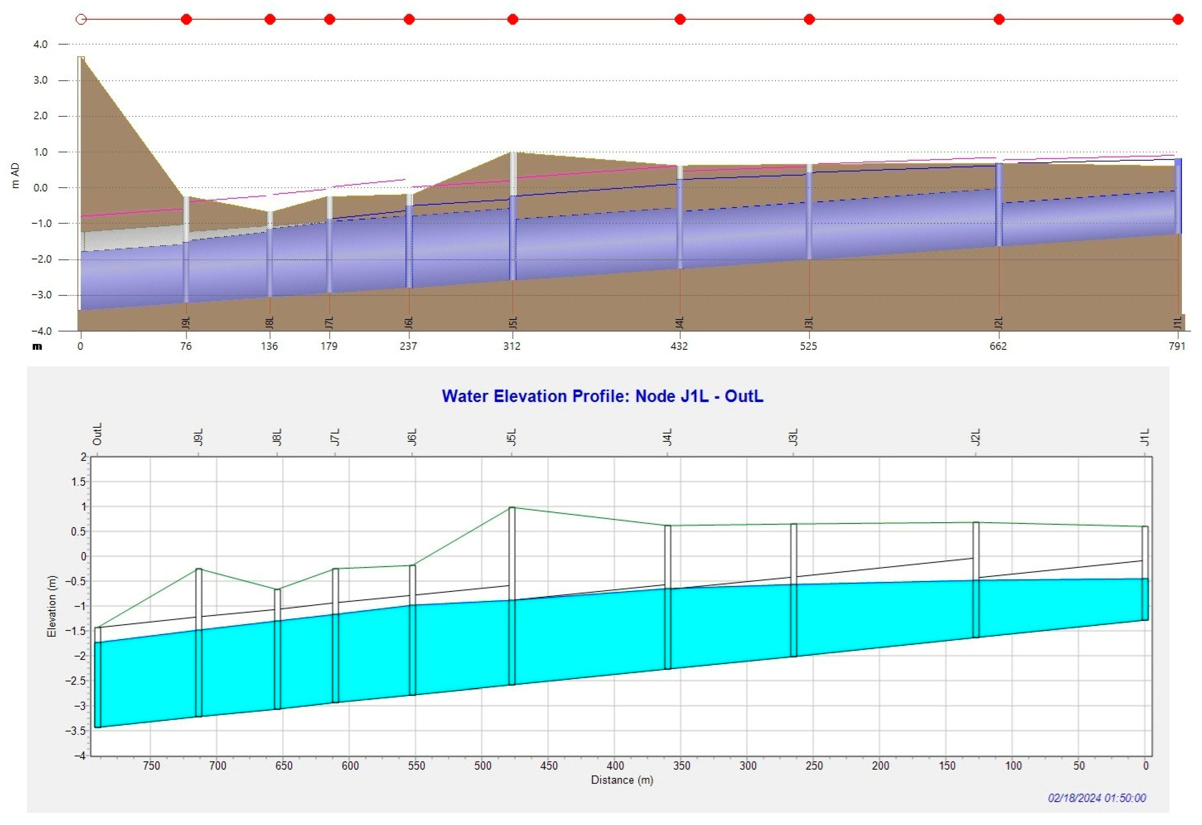
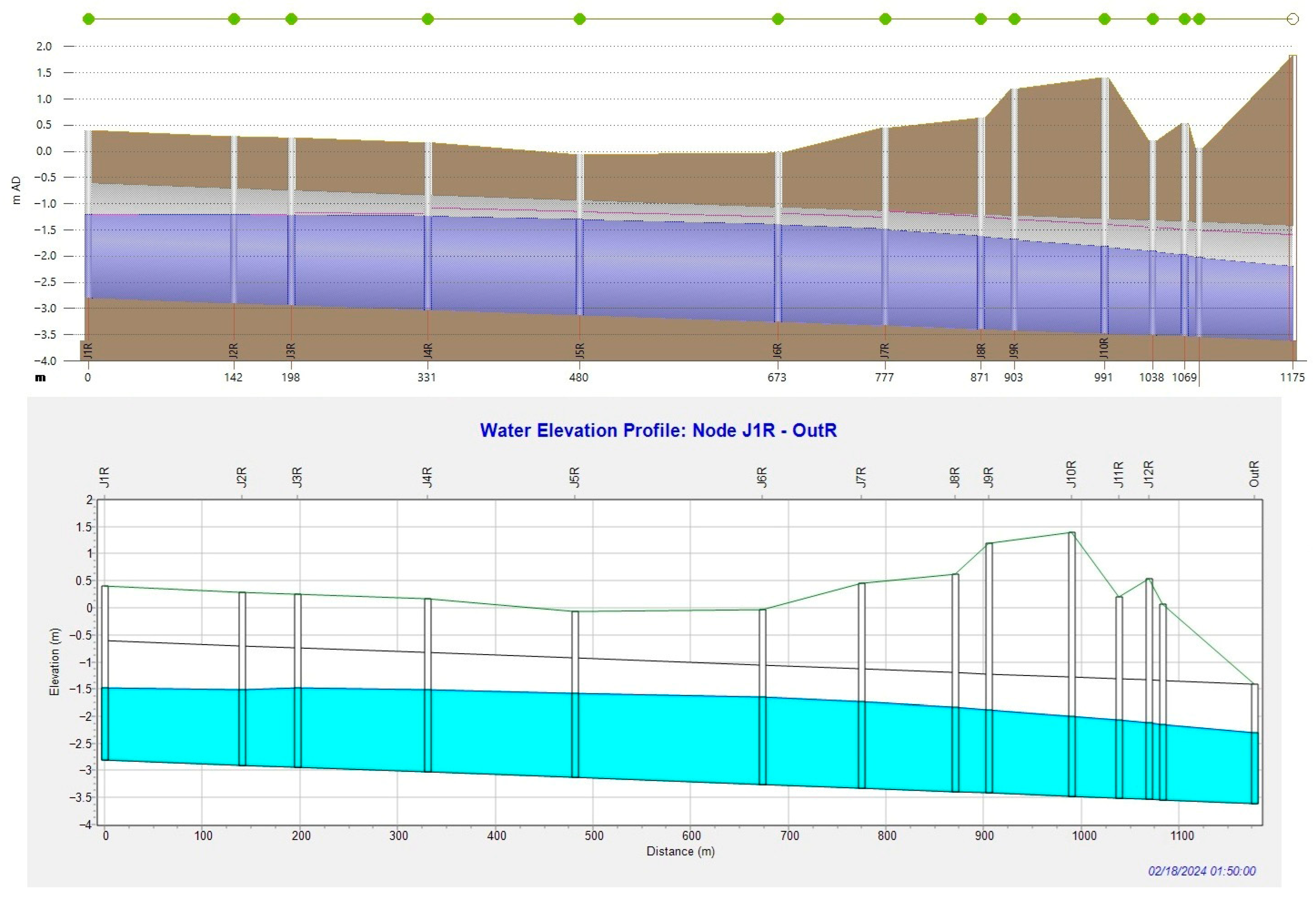
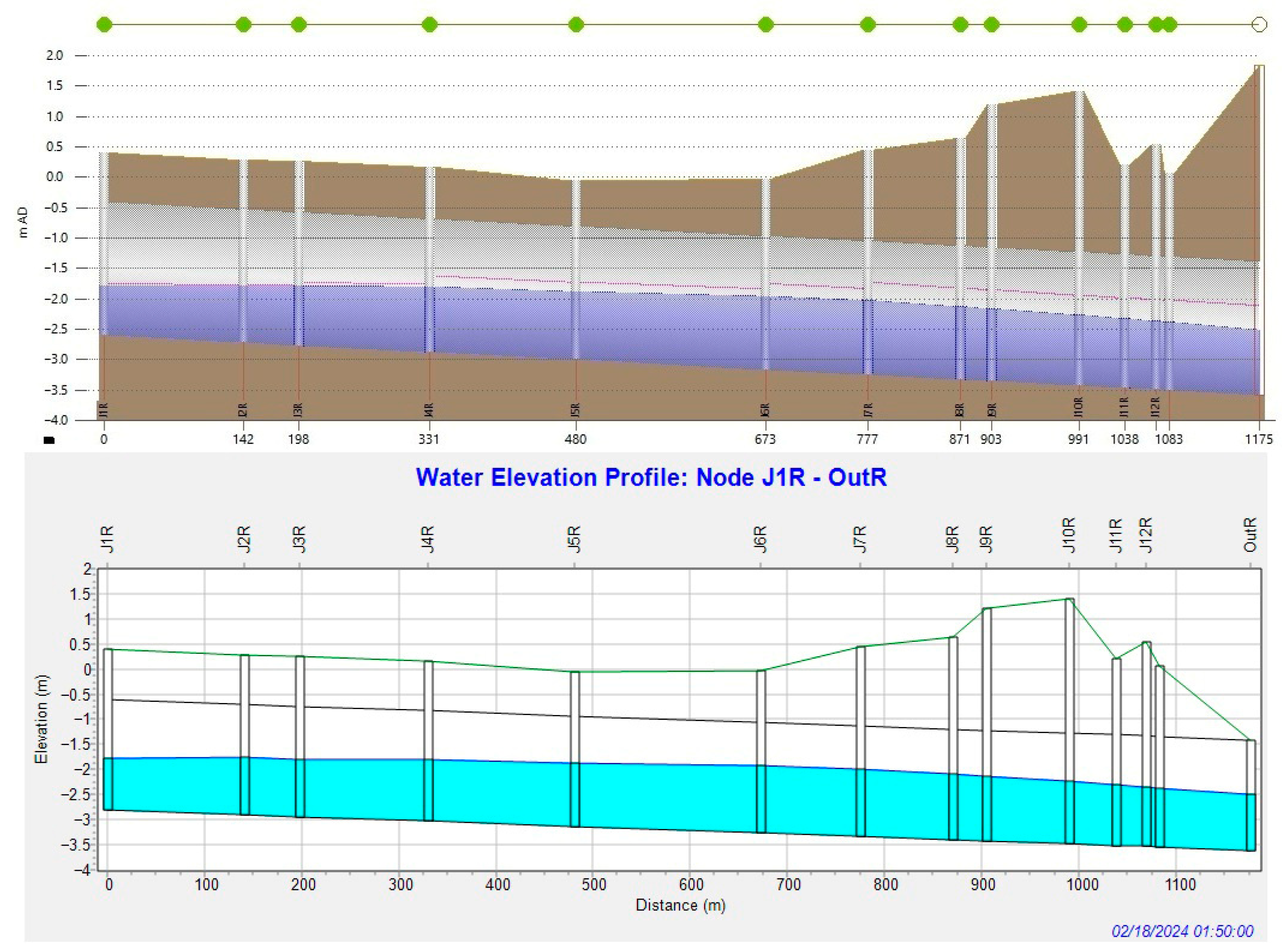
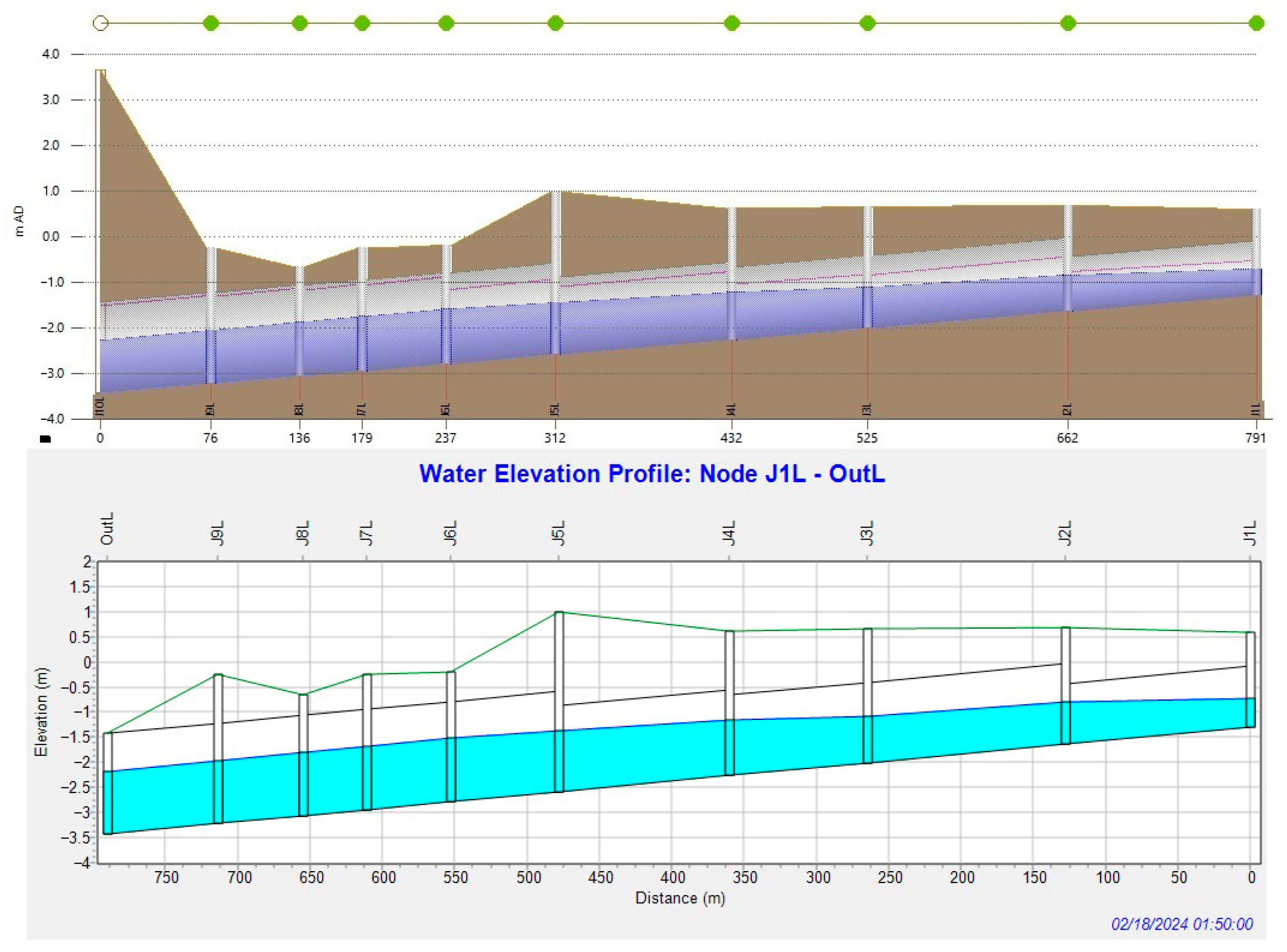
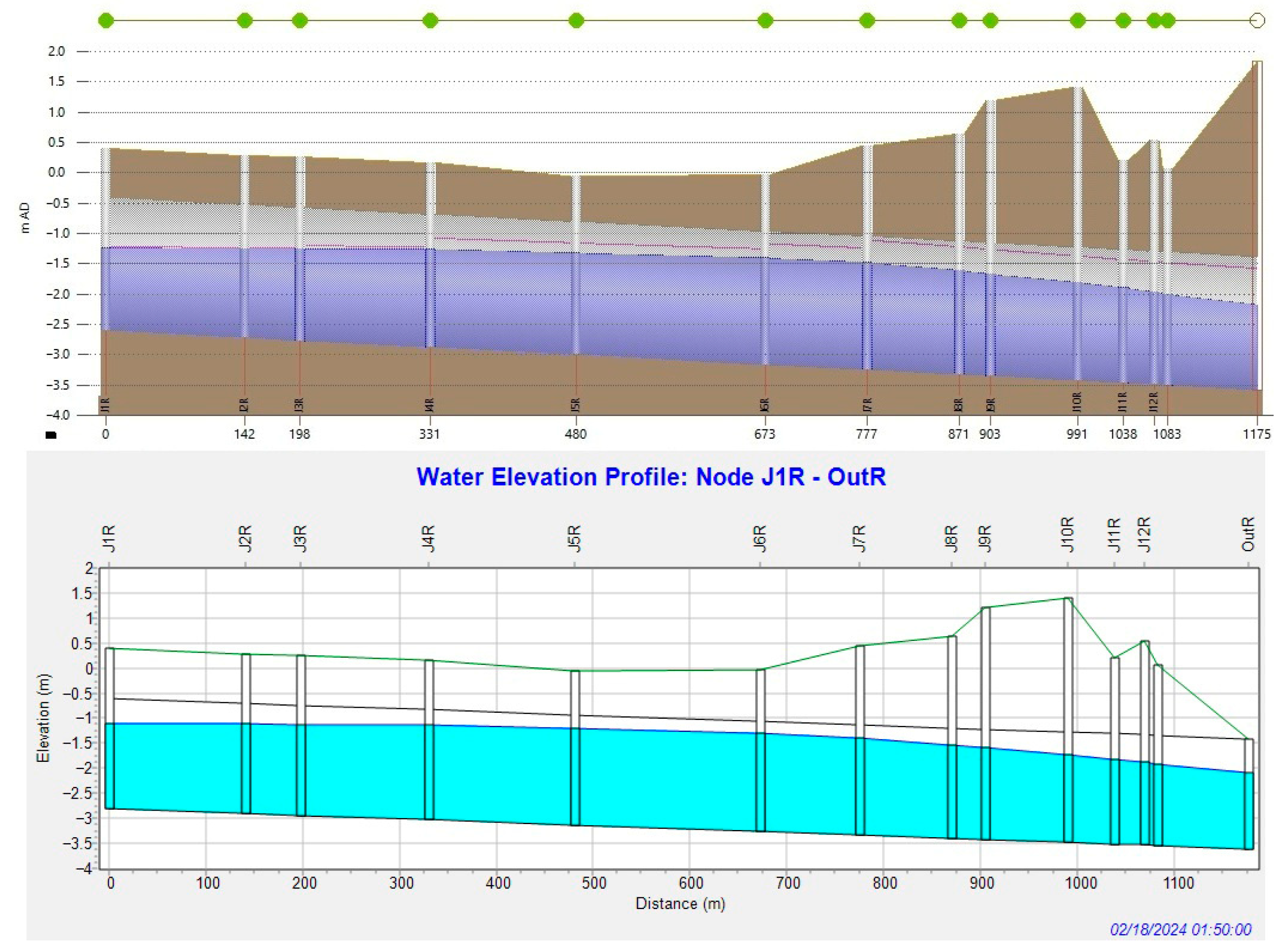
Both software programs replicated the drainage system profile closely (Figure 15, Figure 16, Figure 17 and Figure 18), showing similar values of relative depth at peak flow in the left segment of the drainage system. However, the right segment had higher values than the benchmark (EPA-SWMM 5.2 results; Figure 17 and Figure 18), especially for the rainfall events T20Y-2H and T30Y-3H.
Regarding the relative depth at peak flow (Figure 19), a greater difference lies in the design rainfall event (T10Y-3H, MAE = 0.11), getting smaller for weaker events (T5Y-3H, MAE = 0.08) and stronger events (T20Y-3H, MAE = 0.08 and T30Y-3H, MAE = 0.04). The tendency to reduce MAE values for the 20- and 30-year return period rainfall is mainly due to pressurized conduits, and the condition to set the values at 1 when the relative depth at peak flow results in values greater than one.
The peak flow in the drainage system shows smaller absolute errors on the first three conduits in the left and right sections and increases towards the end independently of the rainfall event (Figure 20). The drainage system’s response to the T20Y-3H rainfall event resulted in the smallest MAE (0.41 m3/s) compared to T5Y-3H (0.75 m3/s), T10Y-3H (0.41 m3/s), and T30Y-3H (0.52 m3/s).

3.3. Comparison C—Scenario S2 in InfoWorks ICM 2021.9 and EPA-SWMM 5.2

This comparison scheme builds on the simulation scenario S1 to explore the effect of including SUDS objects as a proportion of the areas of each sub-catchment (details in Appendix C.5). The SUDS/LID objects used are explained in Section 2.13. As in S1, the EPA-SWMM 5.2 Model was taken as the benchmark for comparison purposes. Figure 21, Figure 22, Figure 23 and Figure 24 show a reduction in the water depth in the pipes to the point that none of the rainfall events considered in this study caused pressurization of the conduits.
Consequently, the 30-year return period rainfall (T30Y-3H) presents the highest value of MAE amongst the events (MAE = 0.10) for the relative depth at peak flow. This was mainly because of the absence of pressurized conduits, which produced the least error in Comparison B due to the assignment of relative depth at peak flow values equal to 1 when pressurization occurs. The rainfall T5Y-3H showed a MAE = 0.05, T10Y-3H resulted in MAE = 0.07, and the T20Y-3H event obtained a MAE = 0.09.
The implementation of the LID/SUDS objects was represented as proportions of the area of each sub-catchment, as detailed in Appendix C.5. Both EPA-SWMM 5.2 and InfoWorks ICM 2021.9 displayed an average reduction in the relative depth at peak flow values of 21% (S.D. = 5%) and 37% (S.D. = 7.9%), respectively (Figure 25). Regarding the peak flow reduction, EPA-SWMM 5.2 shows a decrease of 30% (S.D. = 3.2%), and InfoWorks ICM 2021.9 presents a 43% (S.D. = 3.6%) reduction on average (Figure 26).
When comparing the implementation of LID/SUDS objects (Scenario S2) against the scenario without them (Scenario S1), the runoff quantity continuity obtained from the EPA-SWMM 5.2 status report (Table 11) shows a reduction in the infiltration loss for the T5Y-3H and T10Y-3H rainfall events of 7.6% and 4.3%, respectively, and an increase for T20Y-3H and T30Y-3H of 0.2% and 1.6%, respectively. The surface runoff has decreased on average by 30.3% for all rainfall events. The final storage has an average increase of 8.5 times for all rainfall events.
The infiltration loss decreases for the smallest rainfall events due to the net effect of the green roofs trapping water, bioretention cells storing water, and permeable pavement exfiltrating water. For stronger rainfall events, some LID objects experience saturation, redirecting the water to natural soils. In the case of permeable pavements, more water gets exfiltrated, resulting in more direct infiltration, which leads to more infiltration loss.

3.4. Comparison D—Scenario S3 in InfoWorks ICM 2021.9 vs. Scenario S3 in EPA-SWMM 5.2, a Comparison Between Approaches

Modeling LID/SUDS objects in EPA-SWMM 5.2 requires a pluvial drainage system, whether existing or hypothetical. In the case of Ganzirri Lake, there is no functional pluvial drainage system in Via Consolare Pompea, the road that receives the runoff from an extensive residential area, causing it to flood with relatively weak rainfall events. Comparison D explores modeling a highly urbanized settlement, considering LID/SUDS Objects with a 2D approach as an alternative to model urbanized settlements without a drainage system.
The specific issue of stagnation points is not addressed by the 2D LID/SUDS adaptations. The latter makes sense as stagnation points result from impermeable land covers surrounded by impermeable walls, which are unaffected by the 2D adaptations for LID/SUDS directly.
Additionally, the 2D LID/SUDS adaptations did not significantly reduce the statistics of the 2D simulation of the base scenario (S0) (Table 12). Consequently, the changes in the maximum water depth and speed maps were imperceptible to the eye. Therefore, no maps are shown in this section. Nevertheless, the highlighted values to explore are in the volume balance report (Table 13) when applying 2D LID/SUDS adaptations on the real case (S0) in the intervention area. The effects of the LID/SUDS objects are explained clearly in terms of the proportion of inflow that has turned into infiltrated volume by the different adaptations and have been modeled in the intervention area, which is the residential zone between Via Consolare Pompea and Panoramica del Stretto.
In this case, the 2D simulations increased the average infiltration volume among all rainfall events by 62%, mainly due to bioretention cells, which were distributed in 30% of the available vegetated area (Figure 27) within the limits of the urban sub-catchments (intervention zone; Figure 4). The decrease in the infiltration volume by semipermeable areas from scenarios S0 and S3 is due to the applied LID/SUDS Strategy, which turns 30% of available green open spaces of each sub-catchment into bioretention cells.
When comparing the maximum depth and speed values extracted from the reference points on the grid, scenario S0 (no SUDS) and S3 (with SUDS) show minimal changes (Table 14).
Implementing 2D LID/SUDS adaptations resulted in slight changes in the inundated area compared to the case study’s present state (Table 15). From a total of 154.91 Ha of the 2D domain, the reduction of inundated area between the present state and a LID/SUDS implemented state is 1.69 Ha on average amongst all rainfall events.

4. Discussion

This work aims to build on the existing knowledge on representing urban features in a highly urbanized settlement, such as Ganzirri Lake and its surroundings. The use of different software packages has provided insight into the advantages and limitations for future users in a complex area. The models and comparison also explored using LID/SUDS objects when implemented as 1D and 2D objects.
The lack of a pluvial drainage system and the presence of a protected water body, such as Ganzirri Lake, resulted in a case study with external limitations to be considered when applying modeling techniques. In addition, the models constructed in EPA-SWMM 5.2, HEC-RAS 6.2, and InfoWorks ICM 2021.9 delivered an opportunity to explore the functionality and performance of LID/SUDS objects to reduce the impacts of pluvial flooding.

4.1. InfoWorks ICM 2021.9 vs. HEC-RAS 6.2

This comparison highlights the effect of the representation of buildings in each software and its impact on the simulation and results. As explained in Section 2.9, four methods are cited in the bibliography to represent buildings: voids in the mesh (BV), solid wall conditions on the boundaries (BSW), the building resistance method (BR), and the building block method (BB). In the HEC-RAS 6.2 model, BSW, BR, and BB were employed altogether. In the InfoWorks ICM 2021.9 model, the buildings were represented using the BV approach.
When comparing the statistics of the 2D simulation with HEC-RAS 6.2 and InfoWorks ICM 2021.9, there is a significant difference between the maximum water depth value calculated with both programs on the 2D domain (Table 8). The standard deviation of water depth values shows a high dispersion due to a small section with a considerable water depth. Both models were constructed with the same shapes as data input. The main difference in their implementation was the representation of buildings. Therefore, in HEC-RAS 6.2, the high density of buildings that do not follow a structured distribution pattern (aligned or staggered), the implementation of the BB approach to represent buildings, and very narrow spaces between them result in small grid elements surrounded by impermeable objects, allowing unrealistic water heights.
Additionally, the shape of buildings downloaded from OpenStreetMap presented overlapping polygons on their perimeter, and when the BB method was applied, HEC-RAS 6.2 raised these sections twice (Figure 28).
The water depth maps (refer to Figure 10, Figure 11, Figure 12 and Figure 13) presented particular areas with values above 1.5 m, which were labeled as unusual (hence the different palette of colors). Exploring in further detail, these unusual depths were mainly a result of the approach used to represent buildings, which produced the same effect despite being different between the software used.
In InfoWorks ICM 2021.9, the BV approach creates “voids” in the mesh on the building’s footprint, and the perimeter of each void is considered a wall of infinite height. Therefore, cells are “trapped” between infinite-height walls on impermeable soil, causing water to stagnate and reach these unrealistic heights. On the other hand, HEC-RAS 6.2 employs a combination of the BSW, BR, and BB representation methods. The stagnation occurs due to the BB strategy lifting the topography to create the block, and the runoff gets stagnated between blocks and impermeable surfaces (see Figure 29).
When exploring the max depth and speed values extracted from the reference points (refer to Figure 14a,b), no common characteristics between the reference points (or surroundings) with the least absolute error values could explain the proximity of HEC-RAS 6.2 results to the benchmark. Since the roads and permeable and impermeable areas were represented in similar fashions in both programs, the MAE values differ from each software’s meshing methodology.
InfoWorks ICM 2021.9’s mesh (70,892 cells) is finer than the HEC-RAS 6.2 grid (64,787 cells). The computation cells of each program are configured using different methodologies. HEC-RAS 6.2 uses the Delaunay triangulation as a first step and then constructs Voronoi diagrams from the triangles, creating the cells [44]. According to InfoWorks ICM 2021.9 Help Documentation, the 2D mesh generation uses the Shewchuk triangle method [45], an algorithm to generate a refined 2D mesh based on Delaunay triangulation [46]. Therefore, there will be a difference with respect to the benchmark. This corresponds to similar results in [9] (p. 21).
Depending on the model’s purpose, the differences in maximum depth calculated in HEC-RAS 6.2 compared to InfoWorks ICM 2021.9 can be important or not. Suppose the model’s primary objective is to estimate the extent of pluvial flooding and identify problematic streets or regions. In that case, HEC-RAS 6.2 can be used with the representation adjustments explained in Section 2.9. Nevertheless, suppose a stricter estimation of maximum depths and speeds is required. In that case, the mesh in HEC-RAS 6.2 must be refined even further in areas with roads and permeable surfaces, resulting in slower simulation times.

4.2. EPA-SWMM 5.2 vs. InfoWorks ICM 2021.9

This comparison focuses on the differences between the two programs when used to represent a highly urbanized area using a 1D approach. The differences found in the pluvial drainage network profile of the left and right segments lie in the infiltration methods used for each software. As detailed in Section 2.11, the EPA-SWMM 5.2 model was configured with the curve number method. On the other hand, InfoWorks ICM 2021.9 requires a definition of runoff surfaces within a land use ID for each sub-catchment. Therefore, we used the fixed coefficient method for the runoff surfaces for buildings and roads, and the deficit and constant loss model for permeable areas (refer to Appendix C.3).
The configuration of a land use distribution as absolute areas of each runoff surface for each sub-catchment in InfoWorks ICM 2021.9 is reflected in the differences in the pluvial network profiles of the two programs, especially in the right segment. The left segment of the drainage system is fed by the sub-catchments Bacino 1 to 5, and the right segment by Bacino 6 to 10. The right segment is fed by Bacino 8, which is the largest (16.14 Ha) and one of the most impermeable (72.63% of impermeable area), and by Bacino 9, which is the most impermeable (76.93% of impermeable area). Hence, rapid runoff towards the right segment results in higher relative depth at peak flow values.

4.3. LID/SUDS Modeling in 1D

EPA-SWMM 5.2 has LID control tools, which represent the objects (green roofs, bioretention cells, permeable pavement, and others) as a proportion of the sub-catchment area. InfoWorks ICM 2021.9 has incorporated a SWMM runoff block for InfoWorks networks, allowing it to use LID/SUDS objects characteristics following the same logic as SWMM. Nevertheless, the analysis will be performed using a 1D approach, despite having a 2D network setup. The differences between using EPA-SWMM 5.2 and InfoWorks ICM 2021.9 to model LID/SUDS objects as a proportion of a sub-catchment area are given due to the requirement of InfoWorks ICM 2021.9 to define, at least, three runoff surfaces with the following characteristics: impervious with depression storage, impervious without depression storage, and pervious with depression storage with infiltration characteristics. A definition of surface runoff is not required in EPA-SWMM 5.2.
According to this study’s results, InfoWorks ICM 2021.9 model displayed a greater reduction in the average values of the pluvial drainage network’s peak flow (43% vs. EPA-SWMM 5.2’s 30%) and relative depth at peak flow (37% vs. EPA-SWMM 5.2’s 21%) despite using the same parameters for green roofs, permeable pavements, and bio-retention cells. Under this note, we cannot argue that one program displayed “better” results than the other, as this study’s scope does not include validation with observation data. However, it is crucial to consider each program’s different functionality, primarily referring to the SWMM runoff block in InfoWorks ICM 2021.9, which allows importing an INP file (input file of an EPA-SWMM 5.2 project) directly into a model group in InfoWorks ICM 2021.9. This would not mean that an imported EPA-SWMM 5.2 model in InfoWorks will perform the same as in EPA-SWMM 5.2. As we show in this study, adjustments in the surface runoff characteristics must be considered to refine an imported EPA-SWMM 5.2 model into InfoWorks ICM 2021.9.

4.4. LID/SUDS Modeling in 2D

Recent studies regarding flood risk assessments have gained popularity in urban settlements. These models quantify an urban object’s hazard, exposure, and vulnerability; generally, using hydrodynamic models to estimate exposure and vulnerability as a function of the hazard over a 2D domain [47] (p. 5). Given the usefulness of 2D models in such an important context as flood risk assessments, scenario S3 was thought to address highly urbanized scenarios that include LID/SUDS strategies over a 2D domain and explore their functionality.
The case study of Lake Ganzirri does not have a drainage system. In a 1D domain, this was addressed by designing a hypothetical drainage system. Nevertheless, we wanted to explore the effect of LID/SUDS objects on the propagation of the runoff over a 2D domain. Therefore, a hypothetical drainage system is not helpful in this context.
Using the 2D LID/SUDS adaptations described in this study resulted in minimal reductions in the maximum depth (average of 1.5 mm) and speed maps (average of 0.0125 m/s) on all rainfall events, unperceivable in the maps. The slight differences do not indicate poor efficiency of the LID/SUDS implementation. For scenario S3, the residential area between via Consolare Pompea and Panoramica del Stretto (98.93 Ha) was subject to the implementation of 2D LID/SUDS adjustments on 17.8% of its area, including permeable roads (7.97 Ha) and bio-retention cells (9.8 Ha) coverage. This implementation increased the infiltration volume in the 2D domain by 62% on average for all rainfall events, a decrease of 9.1% of the water flowing outside the boundaries of the 2D zone (normal boundaries). However, the net inflow volume shows a reduction of 1.7% on average for T5Y-3H and T10Y-3H, and an increase of 2.3% on average for T20Y-3H and T30Y-3H. The latter corresponds to the results obtained for Scenario S2, despite being modeled using a 1D approach (5.9% decrease and 0.9% increase on average for the same rainfall events).
The latter can be counterintuitive. However, the consistency of the trends in both software packages with different approaches confirms the behavior of the LID/SUDS Objects. This reflects the efficiency of LID/SUDS for small storms (T5Y-3H and T10Y-3H). The LID/SUDS objects reach their capacity for large storms and start overflowing. This overflow is redirected towards permeable areas or adjacent soils, increasing infiltration.
This study reveals a limitation regarding a 2D green roof adaptation in InfoWorks ICM 2021.9 when using a BV approach to represent buildings as suggested in [34] and used in [48]. To include them, the BV approach could not be used; only the BSW, BR, and BB could be used together, ensuring no single mesh element covers a building footprint and another surface type in the same way as was done in HEC-RAS 6.2. InfoWorks ICM 2021.9 can define the perimeter of a building’s footprint as a breakline, leaving room to explore an adaptation for green roofs further without using the BV approach.

4.5. Inclusion of a Protected Water Body in a Highly Urbanized Area Model

The case study of Lake Ganzirri includes two particular limitations adding up to the complexity of highly urbanized settlements: a protected water body that was used to discharge the runoff with rustic grey infrastructure (gutters and outlets into the lake) that became blocked after being declared a protected body, and a lack of a pluvial drainage system, hence the flood problem on Via Consolare Pompea.
A protected water body in a case study must be considered in the model construction, mainly by preventing runoff from flowing into it. This study considered this in the hypothetical pluvial drainage system design, given that a pipe network is required to construct an EPA-SWMM 5.2 model. The design considered the limitation of not allowing relative depths at peak flow greater than 0.9 for the T10Y-3H rainfall event, so the residential area between Via Consolare Pompea and Panoramica del Stretto will be drained entirely.
Had Lake Ganzirri not been a protected water body, the model could include some outflow into the lake.

4.6. Limitation of Observed Data on the Case Study Area

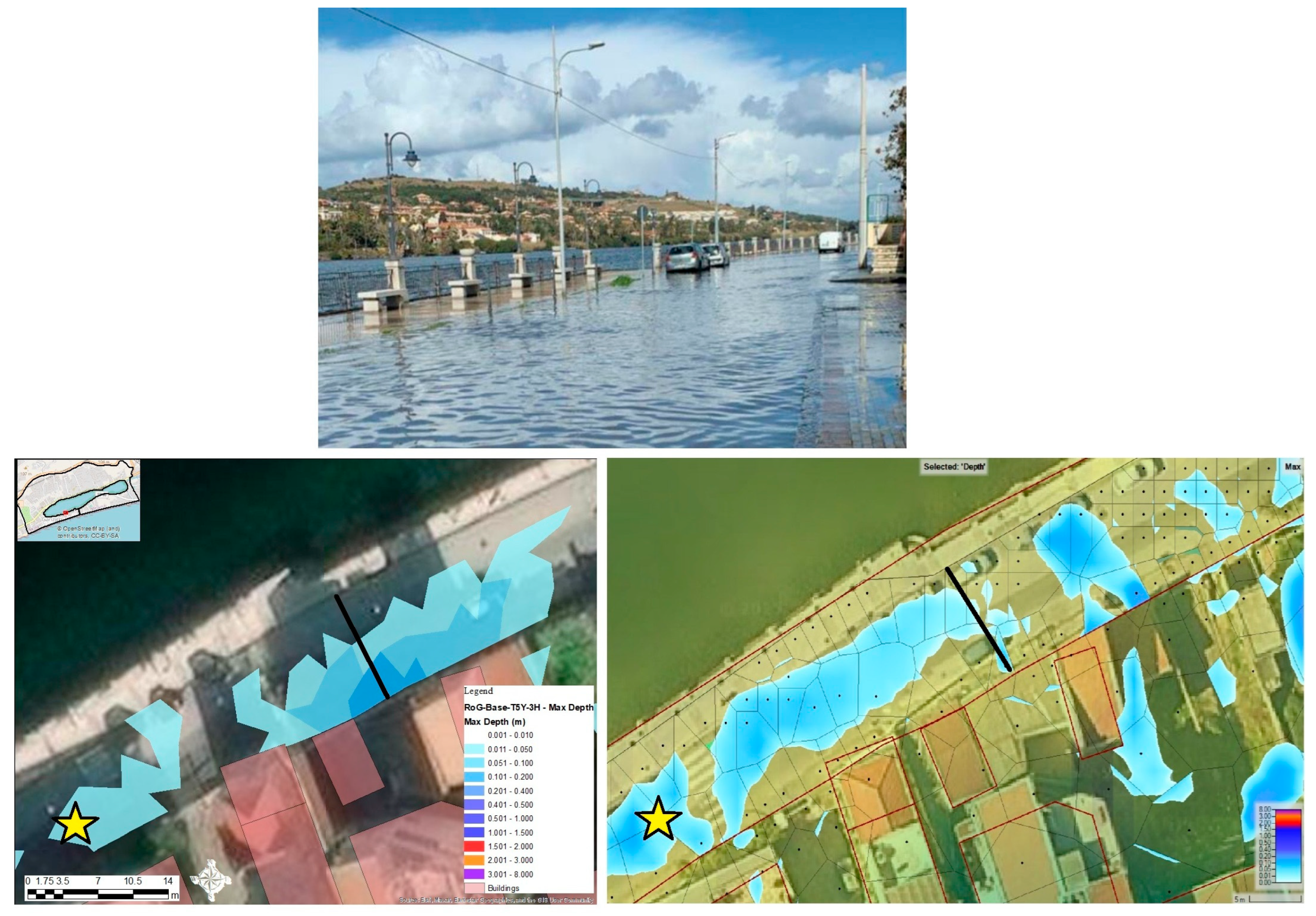
Given the small scale of the Lake Ganzirri case study (100 Ha) there is no observations, records or digital material that could be used to validate the models, except for a 2019 photo extracted from [22] of a section in Via Lago Grande (the southern side of the lake) flooded by a layer of water after a rainfall event (Figure 30).
The reference photo was tracked down (Google Maps coordinates: 38.25813, 15.61260) and was visually compared to the water depth outcomes of scenario S0 in InfoWorks ICM 2021.9 and HEC-RAS 6.2 for the weakest rainfall event. As shown in Figure 30, both models present runoff accumulation. Therefore, the other rainfall events will also cause runoff propagation in the area. On-site measurements were taken on the sidewalk colinear to the lake (0.20 m) and crossing the road (0.08 m). In the same section, the water depth maps of all the rainfall events range from 0.11 to 0.12 m in InfoWorks ICM 2021.9 and from 0.08 to 0.10 m in HEC-RAS 6.2, heights enough to form a layer of water in the location of the reference photo. Nevertheless, the only record of the date of the reference photo is the year 2019, and there is no indication of the intensity of the rainfall event that resulted in the water depth displayed in it. This single record is not solid enough for calibration purposes, but it shows that the models calculated a layer of water in the considered location.

5. Conclusions

The case of Lake Ganzirri presented an interesting case study limited to having a pluvial drainage system where LID/SUDS control elements could be the only solution to mitigate pluvial floods in the area. It included limitations that can be present in other highly urbanized areas, such as unfitting topography to install a pluvial drainage system, highly dense building areas with narrow streets and halls, extended impermeable areas, and protected water bodies restricted from being used as outflows.
The proposed method in this study used a combination of the BSW, BR, and BB referenced methods to represent buildings in HEC-RAS 6.2 that successfully replicated the flow around the buildings, comparable with InfoWorks ICM 2021.9 results. However, the complexity lay in refining the mesh to avoid having cells covering a building’s footprint and other land cover. Fixing the cells represented a time-consuming task requiring manual inspection of each building, and an increase in mesh elements from 58,422 (after the first mesh generation) to 64,787 elements.
We can conclude that the proposed method can represent buildings in HEC-RAS 6.2 without considering them as voids in the mesh in a realistic manner, addressing the limitation of representing green roofs on a 2D domain, since there are no empty meshes in a building’s footprint.
Depending on the purpose of the InfoWorks ICM 2021.9 model, the BV approach is valid if the interest alone is the runoff flow over the surface. It is important to note that InfoWorks ICM 2021.9 calculates an effective area during a simulation run, representing the mesh area considered for the calculations (without mesh elements on the building’s footprint). However, in highly urbanized areas, the large number of buildings in a dense configuration represents an important limitation in studies regarding the water balance of the 2D domain, as the area receiving rainfall in the RoG model can be significantly reduced.
OpenStreetMap information on the presence of roads is presented as lines at the center of the road. However, in RoG modeling, the roads require a finer detail on the mesh to adequately capture the flow at street level. HEC-RAS 6.2 and InfoWorks require polygons to define areas where the mesh needs to be refined, not lines. This represents a significant limitation as the best fit method to create polygons to represent roads is manually digitizing them, which, depending on the size of the case study, can be very time-consuming. Image classification methods are less time-consuming but require high-resolution aerial photos for an adequate classification (i.e., between roads and buildings), often unavailable. Edge detection and segmentation methods also require high-resolution aerial images and clear boundaries. The latter can be a challenge, as in highly urbanized areas, the edges of the roads can be populated with parked cars, trees, and bikeways, making the boundaries difficult to establish. Deep learning approaches can be an alternative, but require significant computational resources and well-labeled training data.
EPA-SWMM 5.2 and InfoWorks ICM 2021.9 have similar tools to include LID/SUDS control objects in a sub-catchment, representing them as a proportion of the area with parameters to control the retention, infiltration, and accumulation features depending on the object (i.e., green roofs, permeable pavement, bioretention cells, etc). When LID/SUDS control objects are assigned as part of the area of a catchment, a lumped approach (1D) is used to compute the rainfall-runoff dynamics. However, in urbanized areas, the runoff flow over a 2D domain can be very different between relatively close locations, as it is highly dependent on the spatial distribution of buildings, roads, permeable and impermeable areas, and existing grey infrastructure in general. Depending on the objective of the assessment of the effectiveness of the implementation of LID/SUDS on an urban hydrological model, a 1D (lumped model) or a 2D approach (rain-on-grid) can be used, considering the following:
-
Efficiency of LID/SUDS control objects on the outflow of the catchment: a 1D approach with surface, pavement, soil, storage, and drainage mat features accordingly is enough using the EPA-SWMM 5.2 and InfoWorks ICM 2021.9 specific tools (LID/SUDS Control Objects).
-
Efficiency of LID/SUDS control objects on the propagation of the runoff: A 2D approach (rain-on-grid) is required to define the urban features using a combination of InfoWorks ICM 2021.9 void polygons, mesh zones, roughness zones, infiltration zones (2D), and general lines (as break lines).
-
There are no LID/SUDS control tools for 2D analysis. Therefore, LID/SUDS Objects must be spatially represented with polygons with 2D adaptations in roughness and infiltration features to replicate their functionality accordingly.
Additionally, maximum depth and speed values are crucial for flood forecasting, nowcasting, and flood risk assessment. Therefore, the mesh should be very detailed in roads (less than 2 × 2 m resolution grid elements). If HEC-RAS 6.2 is considered for predictive modeling on a 2D domain, external assistance to run the model is crucial, as the high level of detail will cause slower simulations.
Lastly, it is important to stress that more validation datasets are necessary for accurate calculations of depths and speeds at localized urban settlements.

Author Contributions

Conceptualization, J.J.S.C. and G.T.A.; Data curation, J.J.S.C.; Formal analysis, J.J.S.C.; Funding acquisition, G.B. and G.T.A.; Investigation, J.J.S.C. and G.B.; Methodology, J.J.S.C.; Project administration, G.B. and G.T.A.; Resources, G.T.A.; Supervision, G.T.A.; Validation, G.B. and G.T.A.; Visualization, J.J.S.C.; Writing—original draft, J.J.S.C. and G.B.; Writing—review and editing, J.J.S.C., G.B. and G.T.A. All authors have read and agreed to the published version of the manuscript.

Funding

The authors declare that this study received funding from the Italian Ministry for Universities and Research (MUIR). This work was developed under the PRIN 2020 (Research Projects of National Interest) project titled “Floods in cities: new INSights for integrating Pluvial floodIng into flood Risk maNaGement plans (INSPRING)”. Grant Number: 2020NTSFXF.

Data Availability Statement

The original contributions presented in this study are included in the article. Further inquiries can be directed to the corresponding authors.

Acknowledgments

This article was produced while attending the PhD programme in PhD in Sustainable Development And Climate Change at the University School for Advanced Studies IUSS Pavia, Cycle XXXIX, with the support of a scholarship co-financed by the Ministerial Decree no. 352 of 9th April 2022, based on the NRRP—funded by the European Union—NextGenerationEU—Mission 4 “Education and research”, Component 2 “From Research to Business”, Investment 3.3, and by the company GetOpen Srl. This work used data from a Scientific Collaboration Agreement between the Department of Urban Planning of the Municipality of Messina and the University of Messina.

Conflicts of Interest

The authors declare that this study received funding from the Italian Ministry for Universities and Research (MUIR). The article was produced while attending the Ph.D. programme in Ph.D. in Sustainable Development And Climate Change at the University School for Advanced Studies IUSS Pavia, Cycle XXXIX, with the support of a scholarship co-financed by the Ministerial Decree no. 352 of 9 April 2022, based on the NRRP—funded by the European Union—NextGenerationEU—Mission 4 “Education and research”, Component 2 “From Research to Business”, Investment 3.3, and by the company GetOpen Srl. The funders had no role in the design of the study; in the collection, analysis, or interpretation of data; in the writing of the manuscript; or in the decision to publish the results.

Appendix A

Appendix A.1. Parameters a, b, and c for DDF Curves

Table A1. Parameters a, b, and c for the DDF curves per return period.
Parameter5-Year10-Year20-Year30-Year
A43.8277253.3339963.6532270.19031
B0.211050.210950.210830.21083
C0.808970.809000.808960.80896

Appendix A.2. Rainfall Intensity

Table A2. Rainfall intensity (mm/h) for different return periods.
t (Min)T5Y-3H
5 Years
T10Y-3H
10 Years
T20Y-3H
20 Years
T30Y-3H
30 Years
00000
104.35.36.36.9
204.95.97.17.8
305.66.88.29
406.68.19.610.6
508.19.911.813
6010.512.815.316.8
7014.918.221.723.9
8025.330.736.640.4
9069.884.9101.3111.7
10069.884.9101.3111.7
11025.330.736.640.4
12014.918.221.723.9
13010.512.815.316.8
1408.19.911.813
1506.68.19.610.6
1605.66.88.29
1704.95.97.17.8
1804.35.36.36.9
Total * (mm)50.060.972.680.0
Note: * Cumulative precipitation for the duration of the rainfall event.

Appendix A.3. Hydrological Features

Table A3. Hydrological features for each sub-catchment.
FeatureBacino 1Bacino 2Bacino 3Bacino 4Bacino 5Bacino 6Bacino 7Bacino 8Bacino 9Bacino 10
Total area (ha) *10.4310.3310.379.715.929.019.1016.147.8410.08
Max elevation (m.a.s.l.)7073.2788280.28179.876.568.571
Min elevation3.52.41.31.21.1110.60.60.9
Longest flow path (m)682.77634.02799.51587.25552.36559.24812.38921.61428.11467.05
Width (m) *152.79162.92129.75165.28107.19161.15112.08175.12183.22215.73
Slope (%) *9.74%11.17%9.59%13.76%14.32%14.31%9.70%8.24%15.86%15.01%
% Imperv62.94%69.40%61.44%72.35%63.18%70.41%64.21%72.63%76.93%54.39%
N-Imperv *0.0110.0110.0110.0110.0110.0110.0110.0110.0110.011
N-Perv *0000000000
Dstore-Imperv (mm) *2.52.52.52.52.52.52.52.52.52.5
Dstore-Perv (mm) *5555555555
%Zero-Imperv *0000000000
Note: * Required in EPA-SWMM 5.2.

Appendix A.4. Infiltration Features

Table A4. Infiltration features for each sub-catchment.
FeatureBacino 1Bacino 2Bacino 3Bacino 4Bacino 5Bacino 6Bacino 7Bacino 8Bacino 9Bacino 10
P (mm)60.960.960.960.960.960.960.960.960.960.9
φ permeable0.30.30.30.30.30.30.30.30.30.3
φ impermeable0.90.90.90.90.90.90.90.90.90.9
φ0.6780.7160.6690.7340.6790.7220.6850.7360.7620.626
Smax (mm)28.95724.09530.16422.04728.76523.38227.95921.85719.05636.309
CN90918992909290929387
d-store perv (mm)5.7914.8196.0334.4095.7534.6765.5924.3713.8117.262

Appendix B

Hypothetical Pluvial Drainage System

Table A5. Junction invert levels.
Upstream (US) NodeDownstream (DS) NodeUS Invert LevelDS Invert Level
J1LJ2L−1.29−1.63
J2LJ3L−1.63−2.01
J3LJ4L−2.01−2.26
J4LJ5L−2.26−2.58
J5LJ6L−2.58−2.79
J6LJ7L−2.79−2.94
J7LJ8L−2.94−3.06
J8LJ9L−3.06−3.22
J9LOutL−3.22−3.43
J1RJ2R−2.80−2.90
J2RJ3R−2.90−2.94
J3RJ4R−2.94−3.03
J4RJ5R−3.03−3.13
J5RJ6R−3.13−3.26
J6RJ7R−3.26−3.33
J7RJ8R−3.33−3.40
J8RJ9R−3.40−3.42
J9RJ10R−3.42−3.48
J10RJ11R−3.48−3.51
J11RJ12R−3.51−3.53
J12RJ13R−3.53−3.54
J13ROutR−3.54−3.61
Table A6. Diameters of the left segment.
LinkDiameter (m)Horizontal Length (m)
C1L1.2127.4908
C2L1.6137.6964
C3L1.695.0382
C4L1.7117.5015
C5L275.0377
C6L257.9111
C7L243.9226
C8L259.4167
C9L276.1756
Table A7. Diameters of the right segment.
LinkDiameter (m)Horizontal Length (m)
C1R2.2140.5288
C2R2.256.772
C3R2.2133.0136
C4R2.2150.7039
C5R2.2192.0743
C6R2.2102.0446
C7R2.295.8336
C8R2.234.5288
C9R2.284.6353
C10R2.248.5773
C11R2.230.6906
C12R2.213.4154
C13R2.294.279

Appendix C

Appendix C.1. Attributes of Spatial Data

The polygon shapefiles representing buildings, roads, and permeable areas must have attributes describing the urban features they represent in HEC-RAS 6.2 and InfoWorks ICM 2021.9. For example, the permeable areas shape file’s table of attributes must have a column “Type” and all the polygons should be classified as “Permeable”. This will make it easier to describe features in HEC-RAS 6.2 when configuring land cover and infiltration layers, as attributes can be assigned by type.
For InfoWorks ICM 2021.9, each polygon representing permeable areas needs an attribute column to assign an identification when used as an “Infiltration surface (2D)” and another identification when used as “Roughness zones”. To ease the model construction process, organizing the shapefiles with extra columns of attributes is suggested before importing them into each software. Table 5 describes a detailed list of suggested attributes and names.
Table A8. Suggested attributes (and names) for shapefiles to ease the import process.
Urban FeatureAttributes for HEC-RAS 6.2Attributes for InfoWorks ICM 2021.9
BuildingsType: Building (all polygons)Category: Void (all polygons) 1.
Void_Id: Void1, Void2,… 2.
Permeable areasType: Permeable (all polygons)Infil_Id: Infil1, Infil2,… 2.
Rough_Id: Rough1, Rough2,… 2.
RoadsType: Roads (all polygons)Mesh_Id: Mesh1, Mesh2,… 2.
Roads perimeterN/ACategory: Break line (all lines) 3.
Notes: 1 Optional. It can be used when importing building polygons to assign them the “Void” category. Alternatively, the category can be assigned directly in InfoWorks via the Open Data Import Center (ODIC). 2 Each polygon has its own identification. 3 Optional. It can be used when importing general lines to assign them the “Break line” category. Alternatively, the category can be assigned directly in InfoWorks via the ODIC. N/A = Not applicable.
The identification helps resolve any warnings that occur during the network validation in InfoWorks ICM 2021.9, especially for potential gaps and overlaps, as the warnings specify which polygons overlap.

Appendix C.2. Parameters for HEC-RAS 6.2 and InfoWorks ICM 2021.9 2D Models

Table A9 details the features of the land, infiltration, and modification layers used in this study for the HEC-RAS 6.2 model.
Table A9. Land cover, infiltration, and modification layers’ parameters for HEC-RAS 6.2.
ParameterValue
CELL SIZE (m)
Land Cover Layer0.1
Infiltration Layer0.1
LAND COVER LAYER
Buildings
ManningsN0.016
Percent Impervious (%) 10
Permeable
ManningsN0.06
Percent Impervious (%)0
Roads
ManningsN0.016
Percent Impervious (%)100
INFILTRATION LAYER
Buildings 2
Initial deficit (mm) 500
Maximum deficit (mm)500
Potential Percolation Rate (mm/hr)1.25
Permeable
Initial deficit (mm) 15
Maximum deficit (mm)60
Potential Percolation Rate (mm/hr)3
Roads
Initial deficit (mm) 0
Maximum deficit (mm)0
Potential Percolation Rate (mm/hr)0
MODIFICATION LAYER
Buildings 3
Elevation Value5
Elevation TypeAddValue
Roads 4
Elevation Value−0.2
Elevation TypeAddValue
Notes: 1 This is set to zero to allow the runoff to infiltrate within the building’s footprint (BR Strategy). 2 High infiltration capacity allows the runoff to infiltrate within the building’s footprint (BB Strategy). 3 BB Strategy. 4 Only on Via Consolare Pompea and Via Lago Grande to add detail to main roads.
In addition, refinement regions and break lines were added to the 2D flow area’s geometry by importing the roads’ polygons and perimeters shapefiles, respectively. The refinement regions’ cell sizes X and Y were set to 2 m and the option “enforce 1 cell protection radius” was checked.
The polygons representing the roads surrounding Lake Ganzirri (Via Consolare Pompea and Via Lago Grande) were imported as a modification layer in the terrain file (add modification → polygons → multipoint). They were selected mainly because they are the most affected by floods. Therefore, to refine their representation, a 0.2 m elevation reduction was applied to the RAS Terrain on these polygons to represent the presence of the sidewalks.
For InfoWorks ICM 2021.9, the buildings were represented as “void polygons”. The roads require finer mesh elements as they act as an open channel and require different roughness features. Therefore, the road shapefile was imported as a mesh zone (maximum triangle area = 7 m2, minimum element area = 2 m2) and roughness zone (Manning’s N = 0.016 for asphalt). The permeable area considers open green areas with grass, trimmed bushes, and trees. It does not consider artificial grass or parking areas of dwellings with plant pots. This land cover requires roughness characteristics and infiltration features. Therefore, the shapefile for permeable areas was imported as a roughness zone (Manning’s N = 0.06 for light brushes and trees) and an infiltration zone 2D.
The 2D infiltration zone requires the configuration of a 2D infiltration surface to assign infiltration features related to the preferred method. For this study, the selected infiltration type was “fixed” with a runoff coefficient of 0.3 [31]. The rainfall percentage in the 2D infiltration zone was set to 100%. This represents that permeable areas are open without any coverage. Appendix C presents suggested attributes of the spatial data to ease the configuration of land and infiltration layers in HEC-RAS 6.2, and infiltration surfaces (2D) and roughness zones in InfoWorks ICM 2021.9.

Appendix C.3. Runoff Surface Properties for Sub-Catchment Assignment in InfoWorks ICM 2021.9

Table A10 details the runoff surface properties to assign to every sub-catchment in the InfoWorks model.
Table A10. Runoff surface properties for sub-catchment assignment (InfoWorks ICM 2021.9).
Runoff Surface ID1234
DescriptionBuildingsRoadsPermeableResidual Area
Surface TypeImperviousImperviousPerviousUnknown
Routing ModelRAFTSRAFTSRAFTSRAFTS
Runoff routing TypeRELRELRELREL
Runoff routing value0.0110.0160.70.011
Runoff volume typeFixedFixedDefConLossFixed
Fixed runoff coefficient0.90.9n/a0.9
Maximum deficit (mm)n/an/a5n/a
Infiltration loss coefficientn/an/a2.5n/a
Initial loss porosity1 (default)1 (default)1 (default)1 (default)
Initial loss typeAbsAbsAbsAbs
Initial loss value (m)0 (default)0 (default)0 (default)0 (default)

Appendix C.4. Runoff Surface Properties for Sub-Catchment Assignment in InfoWorks ICM 2021.9

Table A11, Table A12 and Table A13 detail the parameters to represent SUDS/LID elements.
Table A11. Parameters for green roofs [33].
ParameterValue
SURFACE
Berm height (mm)500
Vegetation Volume Fraction0.1
Surface Roughness (Manning’s n)0.05
Surface Slope (%)2
SOIL
Thickness (mm)30
Porosity (volume fraction)0.5
Field Capacity (volume fraction)0.3
Wilting point (volume fraction)0.05
Conductivity (mm/hr)25
Conductivity Slope15
Suction Head (mm)110
DRAINAGE MAT
Thickness (mm)10
Void Fraction0.5
Roughness (Mannings n)0.1
Table A12. Parameters for permeable pavements [23].
ParameterValue
SURFACE
Berm height (mm)2
Vegetation Volume Fraction0.0
Surface Roughness (Mannings n)0.1
Surface Slope (%)1.5
PAVEMENT
Thickness (mm)120
Void Ratio (Voids/Solids)0.275
Impervious Surface Fraction0
Permeability (mm/hr)3736
Clogging Factor0
Regeneration Interval (days)0
Regeneration Fraction0
STORAGE
Thickness (mm)340
Void Ratio (Voids/Solids)0.305
Seepage Rate (mm/hr)100
Clogging Factor0
Table A13. Parameters for bio-retention cells [34].
ParameterValue
SURFACE
Berm height (mm)350
Vegetation Volume Fraction0.2
Surface Roughness (Mannings n)0.13
Surface Slope (%)0.1
SOIL
Thickness (mm)740
Porosity (volume fraction)0.46
Field Capacity (volume fraction)0.4
Wilting point (volume fraction)0.33
Conductivity (mm/hr)230
Conductivity Slope10
Suction Head (mm)17
STORAGE
Thickness (mm)10
Void Ratio (Voids/Solids)0.75
Seepage Rate (mm/hr)0
Clogging Factor0

Appendix C.5. Distribution of Areas per Sub-Catchment for Comparison Scheme C

Table A14. Distribution of areas per sub-catchment for Comparison C.
Sub-CatchmentTotal Area (ha)Buildings (Roof Area) (ha)Green Roofs (ha)Roads (ha)Permeable Pavement (ha)Pervious Area (ha)Bio-retention Cell (ha)Residual Areas (ha)
Basin 110.43-2.070.300.922.711.163.28
Basin 210.33-1.780.641.222.210.953.53
Basin 310.37-1.580.220.792.801.203.78
Basin 49.71-1.250.460.931.880.814.38
Basin 55.92-0.710.390.441.530.652.20
Basin 69.01-1.050.280.511.870.804.52
Basin 79.10-0.780.450.922.280.983.69
Basin 816.14-1.450.821.413.091.338.04
Basin 97.84-0.710.450.521.270.544.36
Basin 1010.08-0.930.410.313.221.383.82

References

  1. Gu, D.; Andreev, K.; Dupre, M.E. Major Trends in Population Growth Around the World. China CDC Wkly. 2021, 3, 604–613. [Google Scholar] [CrossRef]
  2. Jha, A.K.; Bloch, R.; Lamond, J. Cities and Flooding: A Guide to Integrated Urban Flood Risk Management for the 21st Century; The World Bank: Washington, DC, USA, 2012. [Google Scholar] [CrossRef]
  3. Associated Programme on Flood Management. Urban Flood Risk Management—A Tool for Integrated Flood Management; WMO: Geneva, Switzerland, 2008. [Google Scholar]
  4. Azadgar, A.; Gańcza, A.; Asl, S.R.; Salata, S.; Nyka, L. Optimizing Nature-Based Solutions for Urban Flood Risk Mitigation: A Multi-Objective Genetic Algorithm Approach in Gdańsk, Poland. Sci. Total Environ. 2025, 963, 178303. [Google Scholar] [CrossRef] [PubMed]
  5. Berghauser Pont, M.; Haupt, P.; Berg, P.; Alstäde, V.; Heyman, A. Systematic Review and Comparison of Densification Effects and Planning Motivations. Build. Cities 2021, 2, 378. [Google Scholar] [CrossRef]
  6. Kim, H.W.; Mingh-Han, L.; Jun-Hyun, K.; Fouad, J. Examining the Impact of Suburbanization on Surface Runoff Using the SWAT. Int. J. Environ. Res. 2016, 10, 379–390. [Google Scholar]
  7. Salvadore, E.; Bronders, J.; Batelaan, O. Hydrological Modelling of Urbanized Catchments: A Review and Future Directions. J. Hydrol. 2015, 529, 62–81. [Google Scholar] [CrossRef]
  8. Bagheri, A.; Liu, G.-J. Climate Change and Urban Flooding: Assessing Remote Sensing Data and Flood Modeling Techniques: A Comprehensive Review. Environ. Rev. 2025, 33, 1–14. [Google Scholar] [CrossRef]
  9. Amrei, D.; Britta, S. A Systematic Analysis of the Interaction between Rain-on-Grid-Simulations and Spatial Resolution in 2D Hydrodynamic Modeling. Water 2021, 13, 2346. [Google Scholar] [CrossRef]
  10. Hall, J. Direct Rainfall Flood Modelling: The Good, the Bad and the Ugly. AJWR 2015, 19, 74–85. [Google Scholar] [CrossRef]
  11. David, A.; Schmalz, B. Flood Hazard Analysis in Small Catchments: Comparison of Hydrological and Hydrodynamic Approaches by the Use of Direct Rainfall. J. Flood Risk Manag. 2020, 13, e12639. [Google Scholar] [CrossRef]
  12. Pati, A.; Sahoo, B.; Kale, R.V. A Coupled Modeling Approach for Urban Flood Inundation Mapping under Data-Limited Conditions. J. Hydrol. 2025, 661, 133573. [Google Scholar] [CrossRef]
  13. Da Silva Diniz, G.J.; Scudelari, A.C.; De Medeiros, J.D.F. Performance of Low Impact Development Techniques in Flood Hazard Mitigation in a Closed Urbanised Catchment for Extreme Precipitation Events. Urban Water J. 2024, 21, 987–1002. [Google Scholar] [CrossRef]
  14. Ni, T.; Zhang, X.; Leng, P.; Pelling, M.; Xu, J. Comprehensive Benefits Evaluation of Low Impact Development Using Scenario Analysis and Fuzzy Decision Approach. Sci. Rep. 2025, 15, 2227. [Google Scholar] [CrossRef]
  15. Martínez, C.; Vojinovic, Z.; Sanchez, A. Multi-Objective Model-Based Assessment of Green-Grey Infrastructures for Urban Flood Mitigation. Hydrology 2021, 8, 110. [Google Scholar] [CrossRef]
  16. Ortega Sandoval, A.D.; Sörensen, J.; Rodríguez, J.P.; Bharati, L. Hydrologic–Hydraulic Assessment of SUDS Control Capacity Using Different Modeling Approaches: A Case Study in Bogotá, Colombia. Water Sci. Technol. 2023, 87, 3124–3145. [Google Scholar] [CrossRef]
  17. Neumann, J.; Scheid, C.; Dittmer, U. Potential of Decentral Nature-Based Solutions for Mitigation of Pluvial Floods in Urban Areas—A Simulation Study Based on 1D/2D Coupled Modeling. Water 2024, 16, 811. [Google Scholar] [CrossRef]
  18. Kant, C.; Meena, R.S.; Singh, S.K. A Critical Appraisal on Various Hydrological and Hydrodynamic Models. Water Conserv. Sci. Eng. 2025, 10, 24. [Google Scholar] [CrossRef]
  19. Krvavica, N.; Rubinić, J. Evaluation of Design Storms and Critical Rainfall Durations for Flood Prediction in Partially Urbanized Catchments. Water 2020, 12, 2044. [Google Scholar] [CrossRef]
  20. Rangari, V.A.; Umamahesh, N.V.; Bhatt, C.M. Assessment of Inundation Risk in Urban Floods Using HEC RAS 2D. Model. Earth Syst. Environ. 2019, 5, 1839–1851. [Google Scholar] [CrossRef]
  21. Somma, R.; Spoto, S.E.; Giacobbe, S. Geological and Structural Framework, Inventory, and Quantitative Assessment of Geodiversity: The Case Study of the Lake Faro and Lake Ganzirri Global Geosites (Italy). Geosciences 2024, 14, 236. [Google Scholar] [CrossRef]
  22. Chiofalo, N. Efficacia di Interventi di Drenaggio Urbano Sostenibile Nella Mitigaziones del Rischio di Allagamenti Urbani: Il caso del Lago di Ganzirri. Master’s Thesis, Università degli studi di Messina, Messina, Italy, 2019. [Google Scholar]
  23. European Environmental Agency. Directive 2000/60/EC of the European Parliament and of the Council of 23 October 2000 Establishing a Framework for Community Action in the Field of Water Policy. Off. J. Eur. Communities 2000, 1–73. Available online: https://eur-lex.europa.eu/eli/dir/2000/60/oj/eng (accessed on 5 June 2024).
  24. Costabile, P.; Costanzo, C.; Ferraro, D.; Macchione, F.; Petaccia, G. Performances of the New HEC-RAS Version 5 for 2-D Hydrodynamic-Based Rainfall-Runoff Simulations at Basin Scale: Comparison with a State-of-the Art Model. Water 2020, 12, 2326. [Google Scholar] [CrossRef]
  25. Brunner, G. HEC-RAS 2D User’s Manual. 2024. Available online: https://www.hec.usace.army.mil/software/hec-ras/documentation/HEC-RAS_2D_Users_Manual_v6.5.pdf (accessed on 5 June 2024).
  26. Rossman, L.A. Storm Water Management Model Reference Manual Volume II–Hydraulics; National Risk Management Laboratory: Cincinnati, OH, USA, 2017; Volume II. [Google Scholar]
  27. Cozzolino, L.; Varra, G.; Cimorelli, L.; Pianese, D.; Della Morte, R. Friction Decoupling and Loss of Rotational Invariance in 2D Flooding Models. Adv. Water Resour. 2021, 152, 103919. [Google Scholar] [CrossRef]
  28. Yang, J.; Xiang, Y.; Xu, X.; Sun, J. Design Hyetograph for Short-Duration Rainstorm in Jiangsu. Atmosphere 2022, 13, 899. [Google Scholar] [CrossRef]
  29. Bonaccorso, B.; Brigandì, G.; Aronica, G.T. Regional Sub-Hourly Extreme Rainfall Estimates in Sicily Under a Scale Invariance Framework. Water Resour. Manag. 2020, 34, 4363–4380. [Google Scholar] [CrossRef]
  30. Regione Siciliana. Annali Idrologici. Available online: https://www.regione.sicilia.it/istituzioni/regione/strutture-regionali/presidenza-regione/autorita-bacino-distretto-idrografico-sicilia/annali-idrologici (accessed on 30 July 2025).
  31. Chen, W.; Zheng, M.; Gao, Q.; Deng, C.; Ma, Y.; Ji, G. Simulation of Surface Runoff Control Effect by Permeable Pavement. Water Sci. Technol. 2021, 83, 948–960. [Google Scholar] [CrossRef]
  32. Ming, X.; Liang, Q.; Xia, X.; Li, D.; Fowler, H.J. Real-Time Flood Forecasting Based on a High-Performance 2-D Hydrodynamic Model and Numerical Weather Predictions. Water Resour. Res. 2020, 56, e2019WR025583. [Google Scholar] [CrossRef]
  33. Zhu, Y.; Burlando, P.; Tan, P.Y.; Blagojevic, J.; Fatichi, S. Investigating the Influence of Urban Morphology on Pluvial Flooding: Insights from Urban Catchments in England (UK). Sci. Total Environ. 2024, 953, 176139. [Google Scholar] [CrossRef] [PubMed]
  34. Costabile, P.; Costanzo, C.; Ferraro, D.; Barca, P. Is HEC-RAS 2D Accurate Enough for Storm-Event Hazard Assessment? Lessons Learnt from a Benchmarking Study Based on Rain-on-Grid Modelling. J. Hydrol. 2021, 603, 126962. [Google Scholar] [CrossRef]
  35. Schubert, J.E.; Sanders, B.F.; Smith, M.J.; Wright, N.G. Unstructured Mesh Generation and Landcover-Based Resistance for Hydrodynamic Modeling of Urban Flooding. Adv. Water Resour. 2008, 31, 1603–1621. [Google Scholar] [CrossRef]
  36. Mustafa, A.; Szydłowski, M. Application of Different Building Representation Techniques in HEC-RAS 2-D for Urban Flood Modeling Using the Toce River Experimental Case. PeerJ 2021, 9, e11667. [Google Scholar] [CrossRef]
  37. Rossman, L.A.; Huber, W.C. Storm Water Management Model Reference Manual Volume I–Hydrology (Revised); National Risk Management Laboratory: Cincinnati, OH, USA, 2016; Volume I. [Google Scholar]
  38. Paoletti, A. Sistemi di Fognatura e di Drenaggio Urbano: Fondamenti e Nuove Tendenze, 2nd ed.; CUSL: Milano, Italy, 2002. [Google Scholar]
  39. Artina, S. (Ed.) Sistemi di Fognatura: Manuale di Progettazione; Centro Studi Deflussi Urbani: Milano, Italy, 1997. [Google Scholar]
  40. Hellmers, S.; Manojlović, N.; Palmaricciotti, G.; Kurzbach, S.; Fröhle, P. Multiple Linked Sustainable Drainage Systems in Hydrological Modelling for Urban Drainage and Flood Risk Management. J. Flood Risk Manag. 2018, 11, S5–S16. [Google Scholar] [CrossRef]
  41. Hamouz, V.; Muthanna, T.M. Hydrological Modelling of Green and Grey Roofs in Cold Climate with the SWMM Model. J. Environ. Manag. 2019, 249, 109350. [Google Scholar] [CrossRef] [PubMed]
  42. Gülbaz, S.; Kazezyılmaz-Alhan, C.M. An Evaluation of Hydrologic Modeling Performance of EPA SWMM for Bioretention. Water Sci. Technol. 2017, 76, 3035–3043. [Google Scholar] [CrossRef]
  43. Milanesi, L.; Pilotti, M.; Ranzi, R. A Conceptual Model of People’s Vulnerability to Floods. Water Resour. Res. 2015, 51, 182–197. [Google Scholar] [CrossRef]
  44. Development of the 2D Computational Mesh. Available online: https://www.hec.usace.army.mil/confluence/rasdocs/r2dum/6.2/development-of-a-2d-or-combined-1d-2d-model/development-of-the-2d-computational-mesh (accessed on 26 June 2025).
  45. Help|Two Dimensional Flood Routing Basics|Autodesk. Available online: https://help.autodesk.com/view/IWICMS/2025/ENU/?guid=GUID-F4490F8E-108D-4C14-B31A-D01C793668E1 (accessed on 26 June 2025).
  46. Shewchuk, J.R. Triangle: Engineering a 2D Quality Mesh Generator and Delaunay Triangulator. In Applied Computational Geometry Towards Geometric Engineering; Lin, M.C., Manocha, D., Eds.; Lecture Notes in Computer Science; Springer: Berlin/Heidelberg, Germany, 1996; Volume 1148, pp. 203–222. [Google Scholar] [CrossRef]
  47. Ye, C.; Xu, Z.; Lei, X.; Liao, W.; Ding, X.; Liang, Y. Assessment of Urban Flood Risk Based on Data-Driven Models: A Case Study in Fuzhou City, China. Int. J. Disaster Risk Reduct. 2022, 82, 103318. [Google Scholar] [CrossRef]
  48. Costabile, P.; Costanzo, C.; Kalogiros, J.; Bellos, V. Toward Street-Level Nowcasting of Flash Floods Impacts Based on HPC Hydrodynamic Modeling at the Watershed Scale and High-Resolution Weather Radar Data. Water Resour. Res. 2023, 59, e2023WR034599. [Google Scholar] [CrossRef]
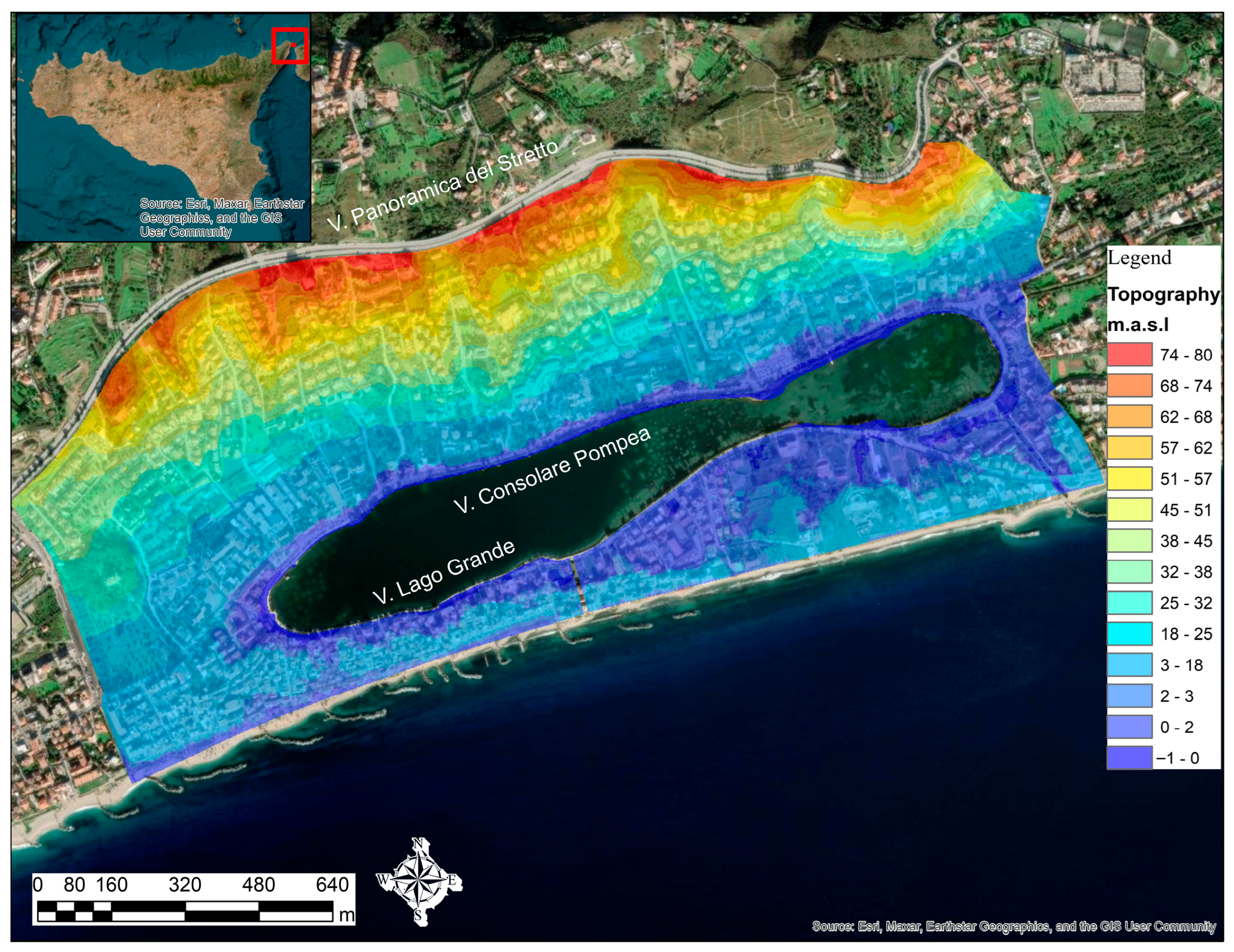
Figure 1. Lake Ganzirri and surrounding topography, Messina, Sicily, Italy (the red square on the upper-left map indicates the location of the study area in Sicily).
Water 17 02978 g001
Figure 2. Lake encasement (left) and channel to the Ionian Sea (right).
Water 17 02978 g002
Figure 3. Simulation scenarios and comparisons.
Water 17 02978 g003
Figure 4. Reference points, sub-catchment delimitation, and 2D zone perimeter.
Water 17 02978 g004
Figure 5. Three-parameter DDF curves for the selected return periods.
Water 17 02978 g005
Figure 6. Designed Chicago hyetographs used for the simulations. Blue = rainfall intensity (mm/h). Red Line = cumulative rainfall (mm).
Water 17 02978 g006
Figure 7. Building representation (top: in HEC-RAS 6.2; middle: real case; bottom: in InfoWorks ICM 2021.9).
Water 17 02978 g007
Figure 8. Illustration of mesh elements covering a building’s footprint and another land cover (circled in yellow).
Water 17 02978 g008
Figure 9. Proposed pluvial drainage system.
Water 17 02978 g009
Figure 10. InfoWorks ICM 2021.9 Maximum Depth Map—T5Y-3H Rainfall Event.
Water 17 02978 g010
Figure 11. HEC-RAS 6.2 Maximum Depth Map—T5Y-3H Rainfall Event.
Water 17 02978 g011
Figure 12. InfoWorks Maximum Depth Map—T30Y-3H Rainfall Event.
Water 17 02978 g012
Figure 13. HEC-RAS 6.2 Maximum Depth Map—T30Y-3H Rainfall Event.
Water 17 02978 g013
Figure 14. Maximum depth (a) and speed (b) on each reference point of the reference simulation scenario (S0) (HEC = HEC-RAS 6.2, INF = InfoWorks ICM 2021.9). (c,d) display paired values of max speed and depth for each reference point and rainfall event on top of zones of people’s vulnerability to floods, indicating high (red), medium (orange), and low (yellow) vulnerability areas as proposed in [43] (p. 189).
Water 17 02978 g014
Figure 15. Pipe profile left segment for the rainfall event T5Y-3H—comparison B.
Water 17 02978 g015
Figure 16. Pipe profile left segment for the rainfall event T30Y-3H—comparison B.
Water 17 02978 g016
Figure 17. Pipe profile right segment for the rainfall event T5Y-3H—comparison B.
Water 17 02978 g017
Figure 18. Pipe profile right segment for the rainfall event T30Y-3H—comparison B.
Water 17 02978 g018
Figure 19. Relative depth at peak flow of each conduit of the drainage system (full line indicates the rainfall event used for the design process of the drainage system)—comparison B. Any value equal to or greater than one is depicted as 1, as it indicates pressurization of the conduit.
Water 17 02978 g019
Figure 20. Peak flow of each conduit of the drainage system (full line indicates the rainfall event used for the design process of the drainage system)—comparison B. Any value equal to or greater than one is depicted as 1, as it indicates pressurization of the conduit.
Water 17 02978 g020
Figure 21. Pipe profile left segment for the rainfall event T5Y-3H—comparison C.
Water 17 02978 g021
Figure 22. Pipe profile right segment for the rainfall event T5Y-3H—comparison C.
Water 17 02978 g022
Figure 23. Pipe profile left segment for the rainfall event T30Y-3H—comparison C.
Water 17 02978 g023
Figure 24. Pipe profile right segment for the rainfall event T30Y-3H—comparison C.
Water 17 02978 g024
Figure 25. Relative depth at peak flow of each conduit of the drainage system (full line indicates the rainfall event used for the design process)—comparison C. Any value equal to or greater than one is depicted as 1, as it indicates pressurization of the conduit.
Water 17 02978 g025
Figure 26. Peak flow of each conduit of the drainage system (full line indicates the rainfall event used for the design process)—comparison C. Any value equal to or greater than one is depicted as 1, as it indicates pressurization of the conduit.
Water 17 02978 g026
Figure 27. Bioretention cells and permeable pavement distribution.
Water 17 02978 g027
Figure 28. Cross-section of a block of buildings showing the double rise on the topography caused by applying the BB method on overlapping polygons representing buildings.
Water 17 02978 g028
Figure 29. Examples of stagnation points (up = InfoWorks ICM 2021.9, bottom = HEC-RAS 6.2, rainfall = T30Y-3H).
Water 17 02978 g029
Figure 30. Reference photo in Vila Lago Grande (top) and the water depth map in InfoWorks ICM 2021.9 (left bottom) and HEC-RAS 6.2 (right bottom) for the T5Y-3H rainfall event and Scenario S0. The star signals the place where the photo was taken. The black lines indicate where on-site measurements of the sidewalk height were taken.
Water 17 02978 g030
Table 1. Hardware details used in the study.
CharacteristicsLaptop 1Laptop 2
BrandASUSLenovo
GPUIntel®CoreTM i7Intel®CoreTM i7
Processor2.40 GHz2.59 GHz
RAM8 GB16 GB
Used forHEC-RAS 6.2 ModelInfoWorks ICM 2021.9 Model and EPA-SWMM 5.2 Simulations
Table 2. Model comparison methodology.
Comparison SchemeSoftware UsedResults—Comparison Methodology
AInfoWorks ICM 2021.9 and HEC-RAS 6.2Statistics of the 2D Simulation—Numeric Comparison
Max Depth and Speed Maps—Visual Comparison
Max Depth and Speed from Reference Points—Mean Absolute Error
Inundated Area—Numeric Comparison
Volume Balance Report—Numerical comparison
BInfoWorks ICM 2021.9 and EPA-SWMM 5.2 Pipe Profile—Visual Comparison
Peak Flow and Relative Height at Peak Flow—Graphical Comparison
Runoff Quantity Continuity—Numeric Comparison
CInfoWorks ICM 2021.9 and EPA-SWMM 5.2Pipe Profile—Visual Comparison
LID/SUDS Objects Proportion or area per sub-catchment
Peak Flow and Relative Height at Peak Flow—Graphical Comparison
Runoff Quantity Continuity—Numeric Comparison
DInfoWorks ICM 2021.9 and EPA-SWMM 5.2Statistics of the 2D Simulation—Numeric Comparison
Max Depth and Speed Maps—Visual Comparison
Volume Balance Report—Numerical comparison
Max Depth and Speed Statistics from Reference Points—Numerical Comparison
Inundated Area—Numeric Comparison.
Table 3. Data provided for this study.
DataFormatDescription
TopographyTIF Files
ASC File
One TIF file with RGB information of 0.0167 × 0.0167 m resolution of the road surrounding the Lake Ganzirri (Via Consolare Pompea and Via Lago Grande) with a 100 m-wide band of the surroundings. This information was extracted from a DTM (Digital Terrain Model).
One TIF file with elevation information of 0.0167 × 0.0167 m resolution of the road surrounding Lake Ganzirri (Via Consolare Pompea and Via Lago Grande) with a 100 m-wide band of the surroundings. This information was extracted from a DSM (Digital Surface Model).
One ASC file of 2 × 2 m resolution of Lake Ganzirri and its surroundings, including the following regions: Casa Bianca, Rione Casalotto, Faro Superiore, Campo Inglese, Contrada Principe, Sant’Agata, Ganzirri, Mortelle, and Torre Faro.
Land/Soil CoverCAD FileCAD file detailing dwellings and buildings, parks, roads, and rustic drainage infrastructure of the case study area.
Table 4. Data preparation.
FeatureType of GIS FeaturesDescriptionUse in HEC-RAS 6.2Use in InfoWorks ICM 2021.9
Topography.Raster (ASC File).2 × 2 m resolution DEM.RAS Terrain.Ground Model Grid.
Perimeter of the study area (excluding the lake).PolygonThe perimeter of the case study area is “donut-shaped” to exclude the lake.2D Flow Area.2D Zone.
Lake Ganzirri Inner Perimeter, East side of the lake, and Coastline 1PolylinesThe perimeter of Lake Ganzirri and the lines where the runoff is expected to flow out of the 2D zone, according to the topography.Boundary condition.N/A
Buildings’ footprint (real geometry) 2PolygonReal geometry of the buildings.Infiltration Layer and Modification Layer in RAS Terrain.Void Polygons
Buildings perimeterPolylinesDelimitation of each representation of the buildings in the study area.Breaklines around each building representation.N/A
RoadsPolygonsRepresentation of the area covered by roads.Refining regions with a cell size of 2 × 2 m.Mesh Zones.
Roughness Zones.
Roads’ perimeterPolylinesDelimitation of each road polygon.Breaklines to limit each road.General line—Category: Break line.
Permeable areasPolygonRepresentation of the area covered by permeable green areas and open spaces with grass and bushes.Land Cover Layer, Infiltration Layer.Roughness Zone.
Infiltration Zone (2D) linked with an Infiltration Surface (2D).
Sub-catchmentsPolygonUrban sub-catchmentsN/ARequired for the 1D–2D interaction model.
Notes: 1 Boundary conditions for HEC-RAS 6.2, defined using the topography to determine the water flowing out of the 2D flow area. 2 Used to calculate the proportion of impermeable area for the sub-catchment’s hydrological features. N/A = Not applicable.
Table 5. HEC-RAS 6.2 advanced time step control settings.
ParameterValue
Adjust Time Step Based on CourantChecked
Maximum Courant2
Minimum Courant0.95
Number of steps below minimum before doubling4
Maximum number of doubling base time steps4
Maximum number of halving base time steps4
Table 6. Distribution of areas per sub-catchment for the reference scenario.
Sub-CatchmentTotal Area (ha)Buildings (Roof Area) (ha)Green Roofs (ha)Roads (ha)Permeable Pavement (ha)Pervious Area (ha)Bio-Retention Cell (ha)Residual Areas (ha)
Basin 110.432.07-1.22-3.87-3.28
Basin 210.331.78-1.87-3.16-3.53
Basin 310.371.58-1.02-4.00-3.78
Basin 49.711.25-1.39-2.68-4.38
Basin 55.920.71-0.83-2.18-2.20
Basin 69.011.05-0.78-2.67-4.52
Basin 79.100.78-1.37-3.26-3.69
Basin 816.141.45-2.23-4.42-8.04
Basin 97.840.71-0.97-1.81-4.36
Basin 1010.080.93-0.73-4.60-3.82
Table 7. LID/SUDS strategy.
LID/SUDS ObjectDescription
Green RoofsAll houses implement green roofs in 100% of their roof area.
Permeable PavementsOn all roads between Via Panoramica and Via Consolare Pompea (excluding these two).
Bioretention cellsOn 30% of the available permeable areas of each sub-catchment between Via Panoramica and Via Consolare Pompea.
Table 8. 2D LID/SUDS Adaptations for Bioretention Cells and Permeable Pavements.
ParameterValue
BIORETENTION CELL
Infiltration Surface (2D)
Infiltration TypeFixed
Fixed Runoff Coefficient0.07
Roughness definition
IDMedium to dense bushes
Number of depth bands1
Roughness 1 (Manning’s n)0.1
PERMEABLE PAVEMENT
Infiltration Surface (2D)
Infiltration TypeFixed
Fixed Runoff Coefficient0.7
Roughness definition
IDAsphalt
Number of depth bands1
Roughness 1 (Manning’s n)0.016
Table 9. Statistics of the 2D simulation—Comparison A (In parentheses, there are the values obtained when exporting HEC-RAS 6.2 results as a raster and processing them using GIS Tools).
InfoWorks ICM 2021.9HEC-RAS 6.2InfoWorks ICM 2021.9HEC-RAS 6.2
Computation Points70,89264,78770,89264,787
Average Simulation time01h37m04h02m01h37m04h02m
Max Depth (m)Max Depth (m)Max Speed (m/s)Max Speed (m/s)
T5Y-3H
Mean0.0210.926 (0.116)0.1840.108
Std. Dev.0.0581.259 (0.190)0.2620.163
Min0.0010.001 (0.001)00
Max2.0837.337 (3.541)2.4842.73
T10Y-3H
Mean0.0230.921 (0.116)0.2090.117
Std. Dev.0.0621.252 (0.190)0.2920.176
Min0.0010.001 (0.001)00
Max2.287.337 (3.541)2.6952.946
T20Y-3H
Mean0.0250.915 (0.116)0.2340.126
Std. Dev.0.0651.249 (0.190)0.3220.189
Min0.0010.001 (0.001)00
Max2.3217.337 (3.541)2.93.147
T30Y-3H
Mean0.0270.912 (0.116)0.2490.131
Std. Dev.0.0671.247 (0.190)0.3390.196
Min0.0010.001 (0.001)00
Max2.3947.337 (3.541)3.1273.263
Table 10. Mean Absolute Error (MAE) between InfoWorks ICM 2021.9 (the benchmark) and HEC-RAS 6.2.
Rainfall EventMAE Depth (m)MAE Speed (m/s)
T5Y-3H0.0640.446
T10Y-3H0.0710.506
T20Y-3H0.0800.589
T30Y-3H0.0890.625
Table 11. Runoff quantity continuity from EPA-SWMM 5.2 status report—scenario S2 (scenario S1 in parentheses, - represents no value).
T5Y-3HT10Y-3HT20Y-3HT30Y-3H
Initial LID Storage (mm)24.357 (-)24.357 (-)24.357 (-)24.357 (-)
Total Precipitation (mm)50.0 (50.0)60.9 (60.9)72.6 (72.6)80.0 (80.0)
Evaporation Loss (mm)0.0 (0.0)0.0 (0.0)0.0 (0.0)0.0 (0.0)
Infiltration Loss (mm)16.187 (17.519)17.848 (18.649)19.406 (19.358)20.331 (20.012)
Surface Runoff (mm)19.973 (28.641)26.826 (38.477)34.111 (48.941)38.981 (55.928)
LID Drainage (mm)- (-)0.477 (-)1.635 (-)2.367 (-)
Final Storage (mm)38.859 (4.801)40.821 (4.805)42.315 (4.861)43.248 (4.877)
Table 12. Statistics of the 2D simulation in InfoWorks ICM 2021.9—scenario S3 (in parentheses, values from S0).
Max Depth (m)Max Speed (m/s)
Computation Points70,89270,892
Average Simulation time01h37m01h37m
T5Y-3H
Mean0.019 (0.021)0.173 (0.184)
Std. Dev.0.056 (0.058)0.250 (0.262)
Min0.001 (0.001)0 (0)
Max2.077 (2.083)2.390 (2.484)
T10Y-3H
Mean0.022 (0.023)0.197 (0.209)
Std. Dev.0.061 (0.062)0.279 (0.292)
Min0.001 (0.001)0 (0)
Max2.170 (2.280)2.593 (2.695)
T20Y-3H
Mean0.024 (0.025)0.221 (0.234)
Std. Dev.0.064 (0.065)0.307 (0.322)
Min0.001 (0.001)0 (0)
Max2.315 (2.321)2.791 (2.900)
T30Y-3H
Mean0.026 (0.027)0.235 (0.249)
Std. Dev.0.066 (0.067)0.324 (0.339)
Min0.001 (0.001)0 (0)
Max2.392 (2.394)2.979 (3.127)
Table 13. Scenario S3 volume balance report (m3) comparison with scenario S0 (in parentheses).
T5Y-3HT10Y-3HT20Y-3HT30Y-3H
Rainfall Inflow (m3)62,759 (62,759)80,609 (80,609)85,070 (85,070)98,339 (98,339)
Infiltration (m3)10,782 (6572)13,050 (7858)15,416 (9679)16,622 (10,504)
By Permeable Pavement1191 (0)1424 (0)1755 (0)1904 (0)
By Semipermeable Areas5187 (6572)6202 (7858)7639 (9679)8291 (10,504)
Within intervention area3162378146575054
Outside intervention area2025242129823237
By Bioretention Cells4404 (0)5424 (0)6022 (0)6427 (0)
Normal boundaries (m3)38,389 (42,315)48,372 (53,295)59,444 (65,370)66,463 (72,985)
Infiltration Within Intervention Area (m3)875810,62912,43413,386
Table 14. Scenario S3 reference points statistics comparison with scenario S0 (in parentheses).
InfoWorks ICM 2021.9InfoWorks ICM 2021.9
Reference Points1919
Max Depth (m)Max Speed (m/s)
T5Y-3H
Min0.009 (0.011)0.072 (0.129)
Mean0.081 (0.085)0.419 (0.458)
Max0.285 (0.290)1.202 (1.327)
T10Y-3H
Min0.009 (0.012)0.082 (0.127)
Mean0.087 (0.092)0.479 (0.523)
Max0.292 (0.304)1.385 (1.510)
T20Y-3H
Min0.011 (0.013)0.093 (0.128)
Mean0.094 (0.099)0.541 (0.590)
Max0.311 (0.324)1.554 (1.689)
T30Y-3H
Min0.011 (0.014)0.099 (0.129)
Mean0.098 (0.103)0.579 (0.631)
Max0.320 (0.334)1.651 (1.796)
Table 15. Inundated areas (Ha).
Rainfall EventScenario S0 (No LID/SUDS)Scenario S3 (with LID/SUDS)
T5Y-3H43.5141.87
T10Y-3H48.2246.68
T20Y-3H52.7150.97
T30Y-3H55.3253.48
Disclaimer/Publisher’s Note: The statements, opinions and data contained in all publications are solely those of the individual author(s) and contributor(s) and not of MDPI and/or the editor(s). MDPI and/or the editor(s) disclaim responsibility for any injury to people or property resulting from any ideas, methods, instructions or products referred to in the content.