

A Review of Water Quality Forecasting Models for Freshwater Lentic Ecosystems

 ,
,  ,
,  , and
, and 
Abstract
1. Introduction
- Beginning of the 20th century: the water supply was increased. Many storage dams, irrigation districts, aqueducts, and water supply systems were constructed.
- From 1980 to 1990: CONAGUA (Comisión Nacional del Agua, translated from Spanish) was established as an institution responsible for managing national waters.
- Dawn of the 21st century: The principal emphasis was focused on water sustainability, wastewater treatment, water reuse, and the management of the water of the nation.
- At what time of day should the variable value be measured?
- How often should monitoring be performed?
- What amount of data is required to train the forecasting model?
- The model/method used to create the prediction model;
- The configuration of the model parameters;
- The number of auxiliary variables for predicting the variable of interest;
- The characteristics of the database used;
- The amount of data (used to train and validate the model).
- The surface area;
- The depth (average, maximum, Secchi);
- The amount of incoming and outgoing water;
- The stratification;
- Others.
- Input (predictors) and output (forecasted variables) for each model;
- Model results for no reported multiple forecast horizons or many horizons;
- Comparison or combining with other models, methods, or techniques;
- The monitoring conditions used;
- Which models gave information to replicate their models (including the availability of their datasets).
2. Theoretical Background
2.1. Artificial Intelligence
- Artificial Intelligence (AI): Ability to perform tasks that require human intelligence, like visual or voice recognition, NLP (Natural Language Processing), etc.
- Machine learning (ML): AI that can learn from experience without human intervention. ML is divided into supervised learning, unsupervised learning, and reinforcement learning
- Deep Learning (DL): AI using algorithms inspired by the human brain (neuronal networks)
2.1.1. Machine Learning
- Supervised learning: In this classification, a human provides labeled data to the algorithm, which learns to predict the output from a given input.
- Unsupervised learning: With this method, the algorithm does not require labeled data and tries to search for patterns.
- Reinforcement learning: The methods in this classification use rewards when the algorithm gives the correct output given a specific input, but if it fails, the algorithm receives penalties. These self-training methods repeat this process many times to achieve the desired performance.
2.1.2. Deep Learning
- Feed-forward neural networks: In these ANNs, the data move from the input layer, through the hidden layers, towards the output layer.
- Recurrent Neural Networks (RNN): RNNs are ANNs in which the data from the output layer flows to the input layer.
- Convolutional Neural Networks (CNN): These ANNs have convolutional and pooling layers, which help in feature extraction and pattern recognition. CNNs are specialized in images.
2.2. ARMA Models
- AR: These models just incorporate an autoregressive part and are represented as , where d is an integer and represents the order of the model.
- MA: These models have only the moving average part and are represented as , where q is an integer and represents the order of the model.
- ARMA: These models result from combining AR and MA models. It is represented as .
- ARIMA (Autoregressive Integrated Moving Average): These models integrate the “I” (Integrated) part and are represented as , where d is an integer and represents the order of the integrated part.
- SARIMA (Seasonal Autoregressive Integrated Moving Average): It adds an “S” (seasonal) part and is represented as , where P, D, and Q are integers that represent the order of the seasonal part and S is an integer that represents the seasonal period.
- SARIMAX (Seasonal Autoregressive Integrated Moving Average with Exogenous Regressors): It is a SARIMA model with exogenous regressors, which includes external variables that might influence the time series.
2.3. Water Quality (WQ)
- Physical parameters: turbidity, TDSs (total dissolved solids), etc.
- Chemical parameters: pH, DO (dissolved oxygen), Salinity, Heavy Metals, etc.
- Microbiologic parameters: E. coli, natural parasites, pathogenic bacteria, etc.
3. Materials and Methods
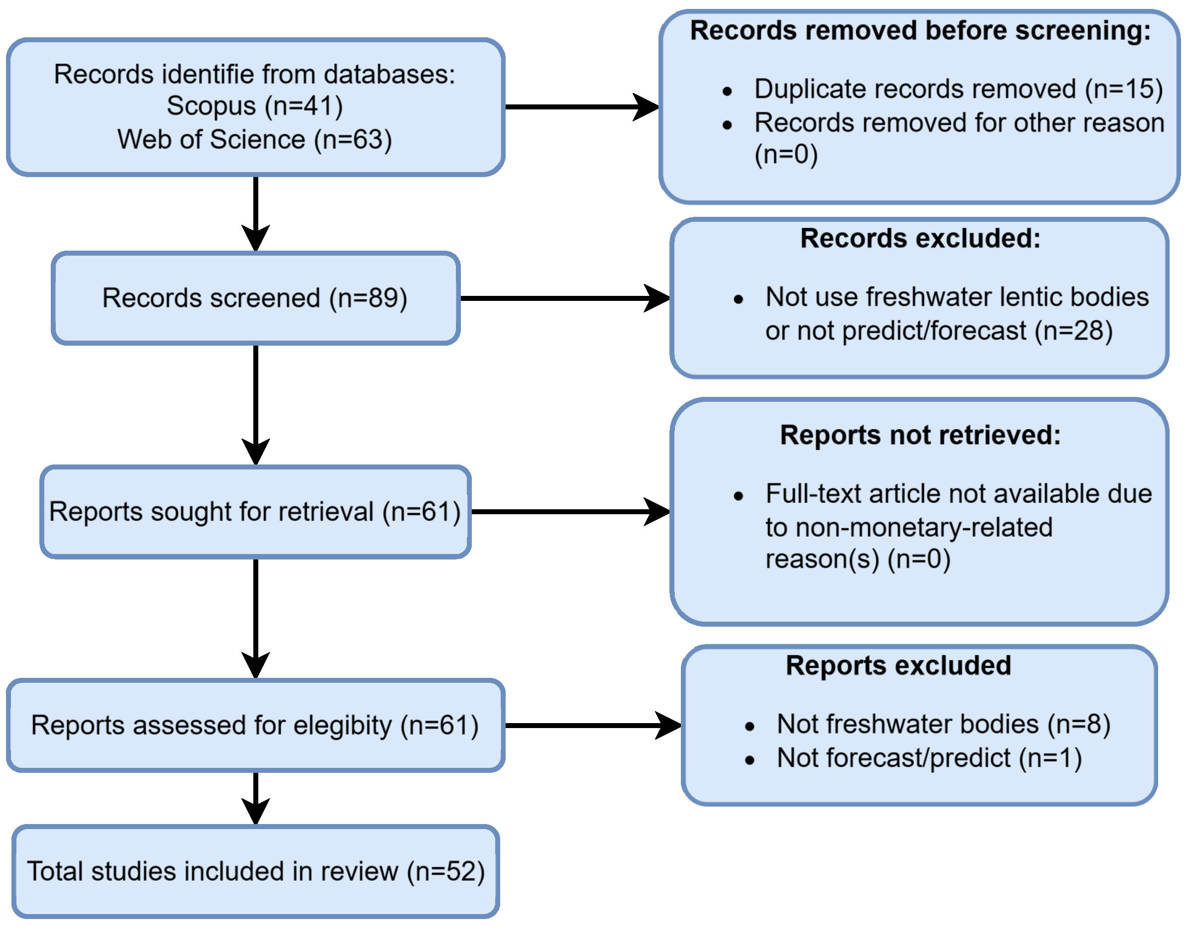
- It has some of the following keywords: freshwater, forecasting or prediction, and water quality.
- The title is related to the “Forecasting or Prediction” of any WQ variable.
- The description mentions developing a forecasting model for any WQ variable of interest.
Research Queries
- TITLE-ABS-KEY (water AND quality AND forecasting AND freshwater) AND (LIMIT-TO (EXACTKEYWORD, “water quality”) OR LIMIT-TO (EXACTKEYWORD, “forecasting”)).
- TITLE-ABS-KEY (water AND quality AND prediction AND freshwater) AND (LIMIT-TO (EXACTKEYWORD, “water quality”) OR LIMIT-TO (EXACTKEYWORD, “prediction”) ).
- water quality forecasting (All Fields) and freshwater (All Fields).
- water quality prediction (All Fields) and freshwater (All Fields).
- The freshwater body of the study was not lentic (i.e., lakes, ponds, dams, reservoirs, etc.).
4. Results
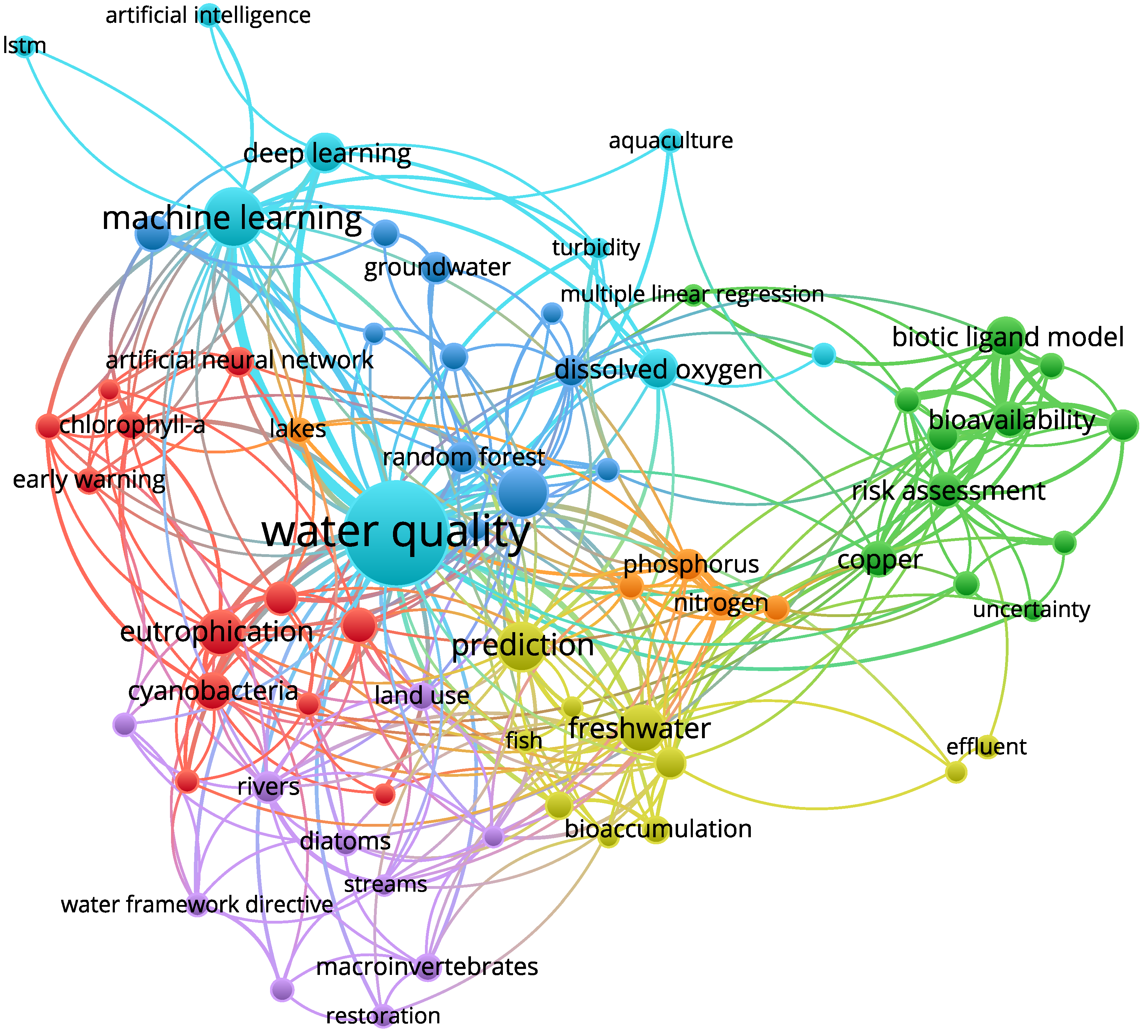
- The co-occurrence of author keywords.
- A full counting method.
- Six as the minimum number of occurrences.
- The research query used was TITLE-ABS-KEY (water AND quality AND prediction AND freshwater) AND (LIMIT-TO (EXACTKEYWORD, “Water Quality”) OR LIMIT-TO (EXACTKEYWORD, “Forecasting”) OR LIMIT-TO (EXACTKEYWORD, “Prediction”) ).
- “Lake” was removed, and “Lakes” was kept.
- “Water Quality Prediction” was removed, and “Prediction” was kept.
- “Modelling” was removed, and “Modeling” was kept.
- The principal types of models are machine learning, deep learning, and Artificial Intelligence.
- The most used models are LSTM, Artificial Neural Network, multiple linear regression, and biotic ligand model.
- Most related variables are dissolved oxygen, chlorophyll alpha (Chl-α), phosphorus, nitrogen, cyanobacteria, and turbidity.
- The types of water analyzed are freshwater and groundwater.
- The principal types of water bodies are lakes, streams, and rivers.
4.1. Which Water Bodies and Variables Are Used in WQ Forecasting?
- In 34 articles, just one freshwater body was used to obtain the data. A few other articles utilized large datasets with data from numerous water bodies: three with more than 100 water bodies, three with more than 1000 water bodies, and two with more than 10,000 water bodies.
- There is a wide period from which datasets were obtained:
- -
- Months: Generally, to obtain data for a specific year period.
- -
- Seasons: Usually to obtain the data characteristics in each season or to avoid some seasons (like winter, when some freshwater bodies freeze).
- -
- A complete year: Habitually to consider a complete cycle.
- -
- More than one year: Usually, articles with datasets with more than one year of data are because the dataset was obtained from a specific organization.
- The principal countries from which WQ variables are forecast are the USA and China, with 12 articles each.
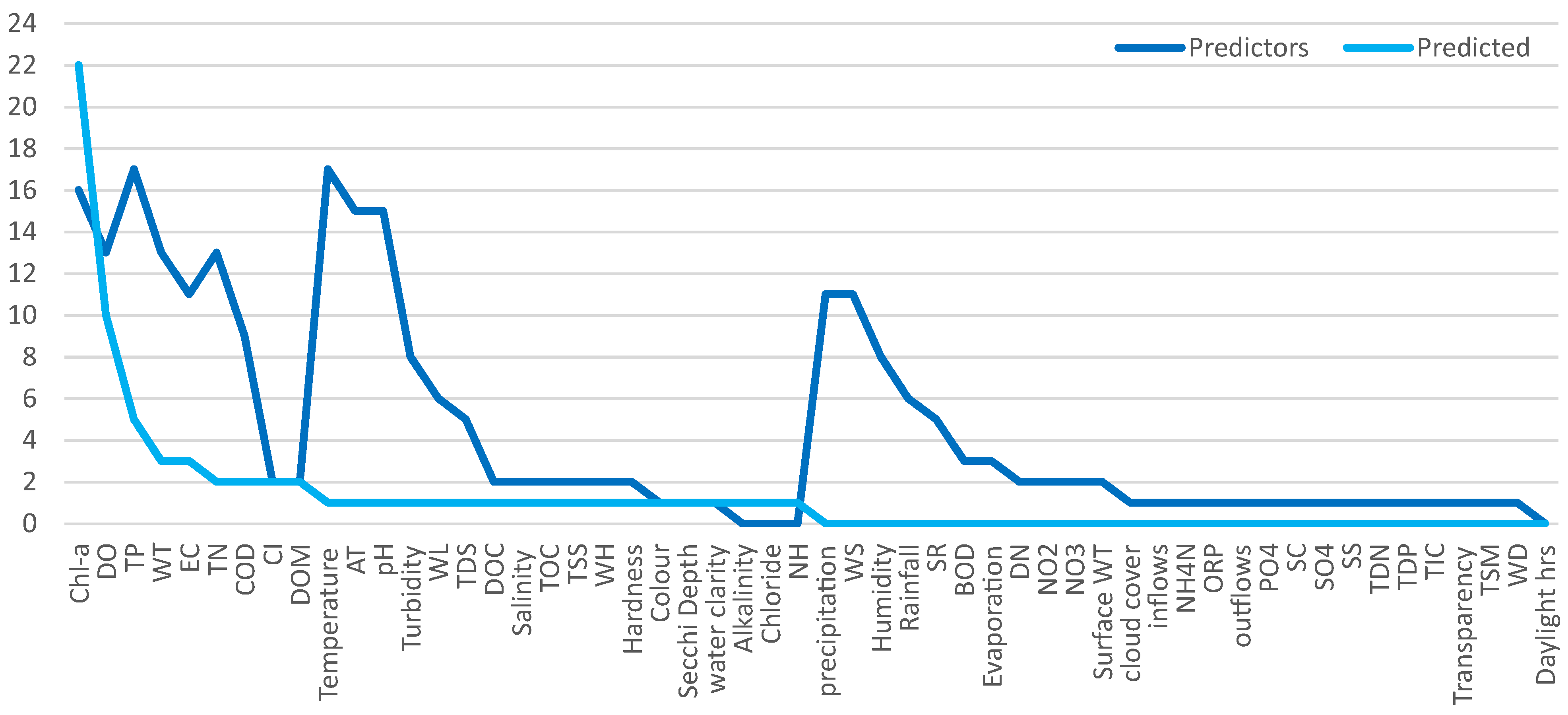
- The water quality variables of greatest interest to forecast are Chl-α (21), DO (8), and TP (5).
- The predictor variables most used are TP and temperature (17 each), Chl-α (16), AT and pH (15), WT and TN (13), and EC and precipitation (11).
4.2. Which Forecasting Methods and Evaluation Metrics Are Used?
- The variables of interest;
- The models implemented;
- The evaluation metrics used.
- The forecasting model presented is the model with the best evaluation metrics, according to the authors of each article.
- Each variable of interest is introduced with its respective evaluation.
- Table 3 only considers the nearest and furthest forecast horizon evaluated (with the evaluation metrics for each horizon).
- With only one forecasted variable: variable of interest—forecasting model—evaluation metrics.
- With two or more forecasted variables: forecasting model—variable of interest (evaluation metrics).
- Forty articles did not evaluate their models with multiple forecast horizons. It does not allow for comparing each performance with models that implement numerous forecast horizons.
- With only one forecasted variable: variable of interest—(evaluation metrics)—forecasting model—nearest forecast horizon: (values for each evaluation metric); farthest forecast horizon: evaluation.
- With two or more forecasted variables: forecasting model—(evaluation metrics)—nearest forecast horizon: variable of interest (values for each evaluation metric); farthest forecast horizon: variable of interest (values for each evaluation metric).
4.3. Which Models or Methods Are Usually Compared or Combined?
4.4. Which Monitoring Conditions Are Usually Implemented?
- No article mentions all three aspects considered.
- Exactly 25 articles mention the monitoring frequency for all or some of the variables used.
- Only three articles indicate the moment when variables are obtained.
- Just seven articles detail the frequency of their models for forecasting.
4.5. How Much Data Is Required to Train, Test, or Validate Forecasting Models?
- 75% (training) and 25% (testing/validation): [27].
- 75% (training), 10% (validation), and 15% (evaluation): [68].
- 60% (training), 20% (validation), and 20% (testing): [51].
- No percentage data: [19] 2/3 (training) and 1/3 (testing); [52] 1000-day data (training), 700-day data (validation); [54] data from 2017 to 2021 (training), data from 2022 (testing); [39] 27-month data (training), 3-month data (validation), and 3-month data (testing); [45] 57 sampling points (training) and 21 sampling points (validation); [46] 107 samples (training) and 70 samples (testing).
4.6. Which Articles Have Made Their Dataset Available?
- The water body of interest is not the same (it is in a different place, has other meteorological conditions, does not have the same physics characteristics, etc.).
- The characteristics of each dataset are different (have different monitoring frequencies, do not monitor the same variables, do not have the same quantity of data, etc.).
- The link to the repository or web page is down;
- A user and password must be accessed (just one case);
- The data will only be available on request;
- Governments and private institutions granted the data.
4.7. Which Articles Give Information About the Configuration Used in Their Forecasting Models?
5. Discussion
5.1. About Water Quality Variables
- The water quality variables of greatest interest to forecast are Chl-α (21), DO (8), and TP (5).
- The predictor variables most used are: TP and temperature (17 each), Chl-α (16), AT and pH (15), WT and TN (13), EC and precipitation (11).
- Just 24 articles used the forecasted variable (at least one) as a predictor variable.
- Only three articles used one variable as a predictor and as a forecasted variable.
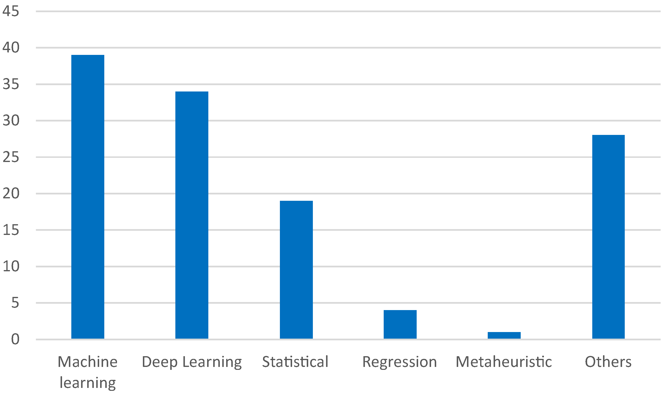
5.2. About the Forecasting Models
- Machine learning (39), including RF (15), SVR (4), GBM (3), XGBoost (3), etc.
- Deep learning (34), including LSTM-based models (10), other NN-based models (10), RNN (3), GTU (3), etc. LSTM and GTU are RNNs, and RNN is a type of NN, respectively. RNN has a total of 16 models, and NN has a total of 26 models.
- Statistical (19): MLR (4), SARIMAX (2), ARIMA, SARIMA, etc.
- Regression models (4): SELM, PLS, SPLS, ELM.
- Metaheuristic (1): WOA.
- Others (28): These includes various models, methods, frameworks, and more.
5.3. About Common Problems
- Of all 52 articles, just 10 articles have made their datasets available.
- Only one article did not introduce the variables to be predicted and/or the auxiliary variables to predict the variable of interest.
- Forty-two articles did not show the configuration of the prediction model.
- Just three articles detailed the exact monitoring conditions. The monitoring moment is usually missing.
- Forty-six articles did not present the monitoring and forecast frequency.
- Only 15 articles gave the percentage or equivalent of data used for training, testing, or evaluating their models.
5.4. How Should the Forecasting Models Be Shared?
- Variables: As seen in previous sections, some information about predictor or forecasted variables are missing, which prevents obtaining data with similar characteristics. To avoid this situation, each variable needs to present the following information:
- -
- The monitoring moment;
- -
- The monitoring frequency;
- -
- The frequency for inputs of the model;
- -
- The output frequency for forecasted variables.
- Dataset: In a similar case, some key information about the dataset used is missing, and the dataset may not be available for downloading. To prevent this situation, a resume is required to give the following details:
- -
- The total data quantity;
- -
- The quantity of missing and replaced data;
- -
- The percentage (or exact quantity of data) used for each train, test, or validation dataset.
- -
- Summary statistics (mean, maximum, minimum values, std, etc.).
- Model: In most cases, key features are missing when searching for information related to the forecasting models, causing a bad or impossible comparison between the models. To avoid this case, the following considerations are required for each forecasting model:
- -
- The exact equations and coefficients obtained (in the corresponding cases),
- -
- The input and output variables;
- -
- The configuration parameters (like hyperparameters for ANNs).
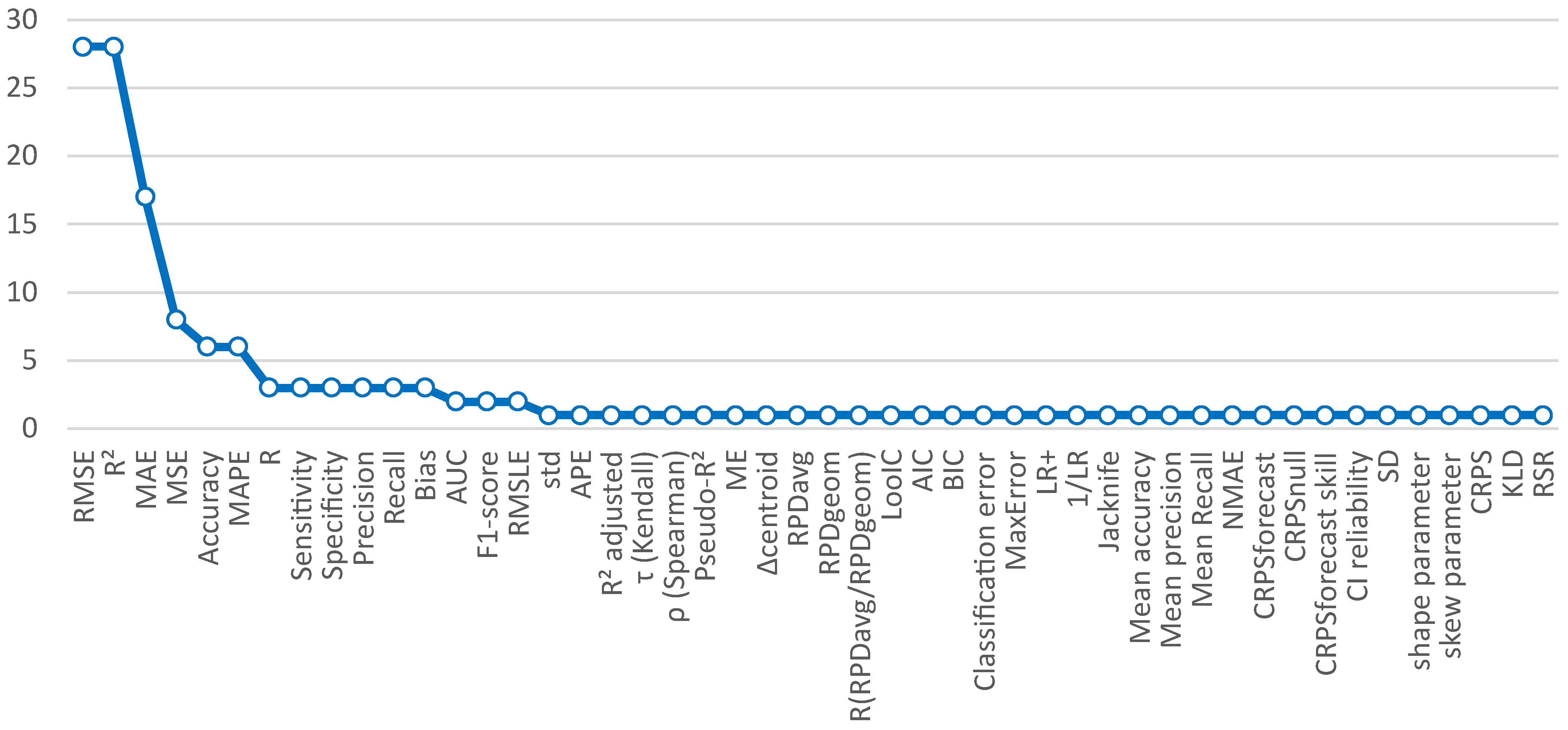
- Evaluation: As seen in Table 2 and Table 3, evaluation metrics have many options. Some metrics are used to obtain specific information. The next evaluation metrics are proposed to ensure a good comparison between different models:
- -
- Error metrics (MAE, MSE, RMSE),
- -
- Correlation coefficient (r),
- -
- Determination coefficient ().
Also, the next evaluation metrics are recommended for classification models:- -
- Precision,
- -
- Accuracy.
5.5. Future Work
- Variation of the dataset size to train: These experiments should answer the question “How many days, months, or years of data is required to have better predictions?” Only [67] cibdycted analyses by varying the size of datasets to train the forecasting models developed.
- Analysing the impact of data frequency: These experiments should answer the question “Which data frequency is required to have a good precision?” It is different to have a dataset with 1000 data points obtained every 12 h (500 continuous days of data) compared to having a dataset with 1000 data points obtained every 7 days (approximately 19 years of data). Additionally, in the specific case of ANN, the input data can be arrays. How much data is required for input arrays to improve WQ forecasting? An array with 10 data points from a database, with a monitoring frequency of 12 h, represents 5 days of data. This case means that data from the previous 5 days supports each data forecast. Increasing or decreasing the data frequency should have an impact on the forecasting values.
6. Conclusions
Author Contributions
Funding
Data Availability Statement
Conflicts of Interest
Abbreviations
| Models | |
| AC-BiLSTM | Attention Convolutional BiLSTM |
| AM | Attention Mechanism |
| BiLSTM | Bidirectional LSTM |
| BMA | Bayesian Model Averaging |
| BN | Bayesian Network |
| BPNN | Backpropagation Neuronal Network |
| CART | Classification and Regression Trees |
| CBiLSTM | CNN-BiLSTM |
| CBiLSTM-AT | CNN-BiLSTM with AM |
| CBOPMM | Cyanobacteria Bloom Occurence Probability Prediction Model |
| CEEMDAN | Complete Ensemble Empirical Mode Decomposition With Adaptive Noise |
| CNN | Convolutional Neuronal Network |
| CT | Classification Tree |
| CVMD | CEEMDAN-VMD |
| DGLM | Dynamic Generalized Linear Model |
| DNN | Deep Neuronal Network |
| FLARE | Forecasting Lake And Reservoir Ecosystems |
| GA | Genetic Algorithm |
| GAM | Generalized Additive Model |
| GANBM | Generalized Additive Negative Binomial Model |
| GAPM | Generalized Additive Poisson Model |
| Gaussian BM | Gaussian Bayesian Network |
| GBM | Gradient Boosting Machine |
| GBR | Gradient Boost Regressor |
| GNN | Graph Neural Networks |
| GNU | Gneural Network |
| GPR | Gaussian Process Regression |
| INLA | Integrated Nested Laplace Approximation |
| IVB | Improved Complete Ensemble Empirical Mode Decomposition With Adaptive Noise-Variational Mode Decomposition-Bidirectional Long Short-term Memory |
| KNN | K-Nearest Neighbors |
| LASSO | Least Absolute Shrinkage and Selection Operator |
| MBPNN | Multilayer Backpropagation Neuronal Network |
| MLP | Multilayer Perceptron |
| MLR | Multiple Linear Regression |
| NBRM | Negative Binomial Regression Model Neuronal Network Bidirectional Long Short-Term Memory |
| NLR | Non Linear Regression |
| NM | Naïve Method |
| PLS | Partial Least Square |
| PLSR | Partial Least Square Regression |
| PRM | Poisson Regression Model |
| PSO | Particle Swarm Optimization |
| QRF | Quantile Regression Forest |
| RF | Random Forest |
| RFR | Random Forest Regressor |
| SELM | Spatial Error Linear Model |
| SPLS | Sparse PLS |
| SVC | Support Vector Classifier |
| SVM | Support Vector Machine |
| SVR | Support Vector Regressor |
| TPS | Two-Phase System |
| VMD | Variation mode decomposition |
| WA | Weighted Average |
| WOA | Whale Optimization Algorithm |
| XGB | Extreme Gradient Boosting |
| XGBRF | Extreme Gradient Boosting with Random Forest |
| ZINBM | Zero-Inflated Negative Binomial Model |
| ZIPM | Zero-Inflated Poisson Model |
| Water Quality Variables | |
| AN | Ammoniacal Nitrogen (mg/L) |
| BOD | Biological Oxygen Demand (mg/L) |
| Chlorophyll alpha | Chl-α (mg/L) |
| CA | Carbon Acumulation |
| COD | Chemical Oxygen Demand (mg/L) |
| CI | Cyanobacterial Index |
| DO | Dissolved Oxygen (mg/L) |
| DOC | Dissolved Organic Carbon (mg/L) |
| DOY | Day of Year |
| EC | Electrical Conductivity (μS/cm) |
| HABs | Harmaful Algal Blooms (ug/L) |
| LAI | Leaf Area Index |
| ORP | Oxidative Reductive Potential (mV) |
| SC | Specific Conductance (μS/cm) |
| SRP | Soluble Reactive Phosphate (mg/L) |
| TOC | Total Organic Carbon (mg/L) |
| TSS | Total Suspended Solids (mg/L) |
| Turbidity | Turbidity (NTU) |
| WH | Wave Height (m) |
| WL | Water Levels (m) |
| Evaluation Metrics | |
| AIC | Aikake Information Criteria |
| BIC | Bayesian Information Criteria |
| DBSCAN | Density-Based Spatial with Clustering of Applications Noise |
| LOF | Local Outliner Factor |
| MAE | Mean Absolute Error |
| MAPE | Mean Absolute Percentage Error |
| MHOE | Mean Higher Order Error |
| MSRE | Mean Squared Relative Error |
| OOB | Out-Of-Bag |
| RMSLE | Root-Mean-Square Log Error |
| RSD | Relative Standard Deviation |
| RSR | Root Mean Squared Error to Standard Deviation |
References
- Krenkel, P.A.; Novotny, V. Water Quality Management; Academic Press Inc.: New York, NY, USA, 1980. [Google Scholar]
- CONAGUA. Estadísticas del Agua en México 2023, March 2024. Available online: https://agua.org.mx/biblioteca/estadisticas-del-agua-en-mexico-2023-conagua/ (accessed on 9 November 2024).
- Brockwell., P.J.; Davis, R.A. Introduction to Time Series and Forecasting; Springer: Cham, Switzerland, 2016. [Google Scholar]
- Odry, A.; Kecskes, I.; Pesti, R.; Csik, D.; Stefanoni, M.; Sarosi, J.; Sarcevic, P. NN-augmented EKF for Robust Orientation Estimation Based on MARG Sensors. Int. J. Control. Autom. Syst. 2025, 23, 920–934. [Google Scholar] [CrossRef]
- Vanegas-Ayala, S.-C.; Barón-Velandia, J.; Romero-Riaño, E. Systematic Review of Forecasting Models Using Evolving Fuzzy Systems. Computation 2024, 12, 159. [Google Scholar] [CrossRef]
- Fatima, S.S.W.; Rahimi, A.A. Review of Time-Series Forecasting Algorithms for Industrial Manufacturing Systems. Machines 2024, 12, 380. [Google Scholar] [CrossRef]
- Tsai, W.-C.; Tu, C.-S.; Hong, C.-M.; Lin, W.-M. A Review of State-of-the-Art and Short-Term Forecasting Models for Solar PV Power Generation. Energies 2023, 16, 5436. [Google Scholar] [CrossRef]
- Mystakidis, A.; Koukaras, P.; Tsalikidis, N.; Ioannidis, D.; Tjortjis, C. Energy Forecasting: A Comprehensive Review of Techniques and Technologies. Energies 2024, 17, 1662. [Google Scholar] [CrossRef]
- Sina, L.B.; Secco, C.A.; Blazevic, M.; Nazemi, K. Hybrid Forecasting Methods—A Systematic Review. Electronics 2023, 12, 2019. [Google Scholar] [CrossRef]
- Akhtar, S.; Shahzad, S.; Zaheer, A.; Ullah, H.S.; Kilic, H.; Gono, R.; Jasiński, M.; Leonowicz, Z. Short-Term Load Forecasting Models: A Review of Challenges, Progress, and the Road Ahead. Energies 2023, 16, 4060. [Google Scholar] [CrossRef]
- Shaheed, H.; Zawawi, M.H.; Hayder, G. The Development of a River Quality Prediction Model That Is Based on the Water Quality Index via Machine Learning: A Review. Processes 2025, 13, 810. [Google Scholar] [CrossRef]
- Yan, X.; Zhang, T.; Du, W.; Meng, Q.; Xu, X.; Zhao, X. A Comprehensive Review of Machine Learning for Water Quality Prediction over the Past Five Years. J. Mar. Sci. Eng. 2024, 12, 159. [Google Scholar] [CrossRef]
- Willard, J.D.; Varadharajan, C.; Jia, X.; Kumar, V. Time series predictions in unmonitored sites: A survey of machine learning techniques in water resources. Environ. Data Sci. 2025, 4, e7. [Google Scholar] [CrossRef]
- Chen, Y.; Song, L.; Liu, Y.; Yang, L.; Li, D. A Review of the Artificial Neural Network Models for Water Quality Prediction. Appl. Sci. 2020, 10, 5776. [Google Scholar] [CrossRef]
- Pan, D.; Deng, Y.; Yang, S.X.; Gharabaghi, B. Recent Advances in Remote Sensing and Artificial Intelligence for River Water Quality Forecasting: A Review. Environments 2025, 12, 158. [Google Scholar] [CrossRef]
- Pan, D.; Zhang, Y.; Deng, Y.; Thé, J.V.G.; Yang, S.X.; Gharabaghi, B. Dissolved Oxygen Forecasting for Lake Erie’s Central Basin Using Hybrid Long Short-Term Memory and Gated Recurrent Unit Networks. Water 2024, 16, 707. [Google Scholar] [CrossRef]
- Ghosh, M.; Thirugnanam, A. Introduction to Artificial Intelligence. In Artificial Intelligence for Information Management: A Healthcare Perspective; Springer: Singapore, 2021; pp. 23–44. [Google Scholar] [CrossRef]
- Page, M.J.; McKenzie, J.E.; Bossuyt, P.M.; Boutron, I.; Hoffmann, T.C.; Mulrow, C.D.; Shamseer, L.; Tetzlaff, J.M.; Akl, E.A.; Brennan, S.E.; et al. The PRISMA 2020 statement: An updated guideline for reporting systematic reviews. Int. J. Surg. 2021, 88, 105906. [Google Scholar] [CrossRef]
- Collins, S.M.; Yuan, S.; Tan, P.N.; Oliver, S.K.; Lapierre, J.F.; Cheruvelil, K.S.; Fergus, C.E.; Skaff, N.K.; Stachelek, J.; Wagner, T.; et al. Winter Precipitation and Summer Temperature Predict Lake Water Quality at Macroscales. Water Resour. Res. 2019, 55, 2708–2721. [Google Scholar] [CrossRef]
- Gao, G.; Xiao, K.; Chen, M. An intelligent IoT-based control and traceability system to forecast and maintain water quality in freshwater fish farms. Comput. Electron. Agric. 2019, 166, 105013. [Google Scholar] [CrossRef]
- Zhao, C.S.; Shao, N.F.; Yang, S.T.; Ren, H.; Ge, Y.R.; Feng, P.; Dong, B.E.; Zhao, Y. Predicting cyanobacteria bloom occurrence in lakes and reservoirs before blooms occur. Sci. Total Environ. 2019, 670, 837–848. [Google Scholar] [CrossRef] [PubMed]
- Peng, Z.; Hu, W.; Liu, G.; Zhang, H.; Gao, R.; Wei, W. Development and evaluation of a real-time forecasting framework for daily water quality forecasts for Lake Chaohu to Lead time of six days. Sci. Total Environ. 2019, 687, 218–231. [Google Scholar] [CrossRef]
- Liu, X.; Feng, J.; Wang, Y. Chlorophyll a predictability and relative importance of factors governing lake phytoplankton at different timescales. Sci. Total Environ. 2019, 648, 472–480. [Google Scholar] [CrossRef]
- Li, Y.; Khan, M.Y.A.; Jiang, Y.; Tian, F.; Liao, W.; Fu, S.; He, C. CART and PSO plus KNN algorithms to estimate the impact of water level change on water quality in Poyang Lake, China. Arab. J. Geosci. 2019, 12, 287. [Google Scholar] [CrossRef]
- Yan, J.; Xu, Z.; Yu, Y.; Xu, H.; Gao, K. Application of a Hybrid Optimized BP Network Model to Estimate Water Quality Parameters of Beihai Lake in Beijing. Appl. Sci. 2019, 9, 1863. [Google Scholar] [CrossRef]
- Derot, J.; Yajima, H.; Jacquet, S. Advances in forecasting harmful algal blooms using machine learning models: A case study with Planktothrix rubescens in Lake Geneva. Harmful Algae 2020, 99, 101906. [Google Scholar] [CrossRef] [PubMed]
- Banerjee, A.; Chakrabarty, M.; Bandyopadhyay, G.; Roy, P.K.; Ray, S. Forecasting environmental factors and zooplankton of Bakreswar reservoir in India using time series model. Ecol. Informatics 2020, 60, 101157. [Google Scholar] [CrossRef]
- Myer, M.H.; Urquhart, E.; Schaeffer, B.A.; Johnston, J.M. Spatio-Temporal Modeling for Forecasting High-Risk Freshwater Cyanobacterial Harmful Algal Blooms in Florida. Front. Environ. Sci. 2020, 8, 581091. [Google Scholar] [CrossRef]
- Zhang, X.; Li, B.; Deng, J.; Qin, B.; Wells, M.; Tefsen, B. Advances in freshwater risk assessment: Improved accuracy of dissolved organic matter-metal speciation prediction and rapid biological validation. Ecotoxicol. Environ. Saf. 2020, 202, 110848. [Google Scholar] [CrossRef]
- Madani, M.; Seth, R. Evaluating multiple predictive models for beach management at a freshwater beach in the Great Lakes region. J. Environ. Qual. 2020, 49, 896–908. [Google Scholar] [CrossRef]
- Thomas, R.Q.; Figueiredo, R.J.; Daneshmand, V.; Bookout, B.J.; Puckett, L.K.; Carey, C.C. A Near-Term Iterative Forecasting System Successfully Predicts Reservoir Hydrodynamics and Partitions Uncertainty in Real Time. Water Resour. Res. 2020, 56, e2019WR026138. [Google Scholar] [CrossRef]
- Dugan, H.A.; Skaff, N.K.; Doubek, J.P.; Bartlett, S.L.; Burke, S.M.; Krivak-Tetley, F.E.; Summers, J.C.; Hanson, P.C.; Weathers, K.C. Lakes at Risk of Chloride Contamination. Environ. Sci. Technol. 2020, 54, 6639–6650. [Google Scholar] [CrossRef]
- Francy, D.S.; Brady, A.M.G.; Stelzer, E.A.; Cicale, J.R.; Hackney, C.; Dalby, H.D.; Struffolino, P.; Dwyer, D.F. Predicting microcystin concentration action-level exceedances resulting from cyanobacterial blooms in selected lake sites in Ohio. Environ. Monit. Assess. 2020, 192, 513. [Google Scholar] [CrossRef]
- Liu, K.; Kong, L.; Wang, J.; Cui, H.; Fu, H.; Qu, X. Two-Phase System Model to Assess Hydrophobic Organic Compound Sorption to Dissolved Organic Matter. Environ. Sci. Technol. 2020, 54, 12173–12180. [Google Scholar] [CrossRef]
- Li, L.; Qiao, J.; Yu, G.; Wang, L.; Li, H.Y.; Liao, C.; Zhu, Z. Interpretable tree-based ensemble model for predicting beach water quality. Water Res. 2022, 211. [Google Scholar] [CrossRef]
- Navarro, M.B.; Schenone, L.; Martyniuk, N.; Vega, E.; Modenutti, B.; Balseiro, E. Predicting Dissolved Organic Matter Lability and Carbon Accumulation in Temperate Freshwater Ecosystems. Ecosystems 2022, 25, 795–811. [Google Scholar] [CrossRef]
- Hadid, N.B.; Goyet, C.; Maiz, N.B.; Shili, A. Long-term forecasting in a coastal ecosystem: Case study of a Southern restored Mediterranean lagoon: The North Lagoon of Tunis. J. Coast. Conserv. 2022, 26, 10. [Google Scholar] [CrossRef]
- Jackson-Blake, L.A.; Clayer, F.; Haande, S.; Sample, J.E.; Moe, S.J. Seasonal forecasting of lake water quality and algal bloom risk using a continuous Gaussian Bayesian network. Hydrol. Earth Syst. Sci. 2022, 26, 3103–3124. [Google Scholar] [CrossRef]
- Chen, W.; Kim, J.; Yu, J.; Wang, X.; Peng, S.; Zhu, Z.; Wei, Y. COD forecasting of Poyang lake using a novel hybrid model based on two-layer data decomposition. Nongye Gongcheng Xuebao/Trans. Chin. Soc. Agric. Eng. 2022, 38, 296–302. [Google Scholar] [CrossRef]
- Carey, C.C.; Woelmer, W.M.; Lofton, M.E.; Figueiredo, R.J.; Bookout, B.J.; Corrigan, R.S.; Daneshm, V.; Hounshell, A.G.; Howard, D.W.; Lewis, A.S.; et al. Advancing lake and reservoir water quality management with near-term, iterative ecological forecasting. Inland Waters 2022, 12, 107–120. [Google Scholar] [CrossRef]
- You, L.; Tong, X.; Te, S.H.; Tran, N.H.; Sukarji, N.H.B.; He, Y.; Gin, K.Y.H. Multi-class secondary metabolites in cyanobacterial blooms from a tropical water body: Distribution patterns and real-time prediction. Water Res. 2022, 212, 118129. [Google Scholar] [CrossRef]
- Martinsen, K.T.; Sand-Jensen, K. Predicting water quality from geospatial lake, catchment, and buffer zone characteristics in temperate lowland lakes. Sci. Total Environ. 2022, 851, 158090. [Google Scholar] [CrossRef]
- Qian, Z.; Cao, Y.; Wang, L.; Wang, Q. Developing cyanobacterial bloom predictive models using influential factor discrimination approach for eutrophic shallow lakes. Ecol. Indic. 2022, 144, 109458. [Google Scholar] [CrossRef]
- Crapart, C.; Finstad, A.G.; Hessen, D.O.; Vogt, R.D.; Andersen, T. Spatial predictors and temporal forecast of total organic carbon levels in boreal lakes. Sci. Total Environ. 2023, 870, 161676. [Google Scholar] [CrossRef]
- Ding, L.; Qi, C.; Li, G.; Zhang, W. TP Concentration Inversion and Pollution Sources in Nanyi Lake Based on Landsat 8 Data and InVEST Model. Sustainability 2023, 15, 9678. [Google Scholar] [CrossRef]
- Gupta, A.; Hantush, M.M.; Govindaraju, R.S. Sub-monthly time scale forecasting of harmful algal blooms intensity in Lake Erie using remote sensing and machine learning. Sci. Total Environ. 2023, 900, 165781. [Google Scholar] [CrossRef] [PubMed]
- Torres-Vera, M.A. Mapping of total suspended solids using Landsat imagery and machine learning. Int. J. Environ. Sci. Technol. 2023, 20, 11877–11890. [Google Scholar] [CrossRef]
- Amieva, J.F.; Oxoli, D.; Brovelli, M.A. Machine and Deep Learning Regression of Chlorophyll-a Concentrations in Lakes Using PRISMA Satellite Hyperspectral Imagery. Remote Sens. 2023, 15, 5385. [Google Scholar] [CrossRef]
- Rodríguez-López, L.; Usta, D.B.; Duran-Llacer, I.; Alvarez, L.B.; Yépez, S.; Bourrel, L.; Frappart, F.; Urrutia, R. Estimation of Water Quality Parameters through a Combination of Deep Learning and Remote Sensing Techniques in a Lake in Southern Chile. Remote Sens. 2023, 15, 4157. [Google Scholar] [CrossRef]
- Harkort, L.; Duan, Z. Estimation of dissolved organic carbon from inland waters at a large scale using satellite data and machine learning methods. Water Res. 2023, 229, 119478. [Google Scholar] [CrossRef]
- Ozdemir, S.; Yildirim, S.O. Prediction of Water Level in Lakes by RNN-Based Deep Learning Algorithms to Preserve Sustainability in Changing Climate and Relationship to Microcystin. Sustainability 2023, 15, 16008. [Google Scholar] [CrossRef]
- Barbosa, C.C.; do Carmo Calijuri, M.; da Silva Anjinho, P.; dos Santos, A.C.A. An integrated modeling approach to predict trophic state changes in a large Brazilian reservoir. Ecol. Model. 2023, 476, 110227. [Google Scholar] [CrossRef]
- Tan, R.; Wang, Z.; Wu, T.; Wu, J. A data-driven model for water quality prediction in Tai Lake, China, using secondary modal decomposition with multidimensional external features. J. Hydrol.-Reg. Stud. 2023, 47, 101435. [Google Scholar] [CrossRef]
- Hwang, S.Y.; Choi, B.W.; Park, J.H.; Shin, D.S.; Lee, W.S.; Chung, H.S.; Son, M.S.; Ha, D.W.; Lee, K.L.; Jung, K.Y. Evaluation of algal species distributions and prediction of cyanophyte cell counts using statistical techniques. Environ. Sci. Pollut. Res. 2023, 30, 117143–117164. [Google Scholar] [CrossRef]
- Villanueva, P.; Yang, J.; Radmer, L.; Liang, X.; Leung, T.; Ikuma, K.; Swanner, E.D.; Howe, A.; Lee, J. One-Week-Ahead Prediction of Cyanobacterial Harmful Algal Blooms in Iowa Lakes. Environ. Sci. Technol. 2023, 57, 20636–20646. [Google Scholar] [CrossRef]
- Nkwalale, L.; Schwefel, R.; Yaghouti, M.; Rinke, K. A simple model for predicting oxygen depletion in lakes under climate change. Inland Waters 2023, 13, 576–595. [Google Scholar] [CrossRef]
- Rirongarti, R.; Sylvestre, F.; Chalie, F.; Pailles, C.; Mazur, J.C.; Nour, A.M.; Barthelemy, W.; Mariot, H.; der Meeren, T.; Poulin, C.; et al. A diatom-based predictive model for inferring past conductivity in Chadian Sahara lakes. J. Paleolimnol. 2023, 69, 231–248. [Google Scholar] [CrossRef]
- Miura, Y.; Imamoto, H.; Asada, Y.; Sagehashi, M.; Akiba, M.; Nishimura, O.; Sano, D. Prediction of algal bloom using a combination of sparse modeling and a machine learning algorithm: Automatic relevance determination and support vector machine. Ecol. Informatics 2023, 78, 102337. [Google Scholar] [CrossRef]
- Talukdar, S.; Shahfahad; Bera, S.; Naikoo, M.W.; Ramana, G.V.; Mallik, S.; Kumar, P.A.; Rahman, A. Optimisation and interpretation of machine and deep learning models for improved water quality management in Lake Loktak. J. Environ. Manag. 2024, 351, 119866. [Google Scholar] [CrossRef] [PubMed]
- Schaeffer, B.A.; Reynolds, N.; Ferriby, H.; Salls, W.; Smith, D.; Johnston, J.M.; Myer, M. Forecasting freshwater cyanobacterial harmful algal blooms for Sentinel-3 satellite resolved U.S. lakes and reservoirs. J. Environ. Manag. 2024, 349, 119518. [Google Scholar] [CrossRef]
- Rodríguez-López, L.; Alvarez, D.; Usta, D.B.; Duran-Llacer, I.; Alvarez, L.B.; Fagel, N.; Bourrel, L.; Frappart, F.; Urrutia, R. Chlorophyll-a Detection Algorithms at Different Depths Using In Situ, Meteorological, and Remote Sensing Data in a Chilean Lake. Remote Sens. 2024, 16, 647. [Google Scholar] [CrossRef]
- Woelmer, W.M.; Thomas, R.Q.; Olsson, F.; Steele, B.G.; Weathers, K.C.; Carey, C.C. Process-based forecasts of lake water temperature and dissolved oxygen outperform null models, with variability over time and depth. Ecol. Inform. 2024, 83, 102825. [Google Scholar] [CrossRef]
- Nanjappachetty, A.; Sundar, S.; Vankadari, N.; Bapu, T.B.B.R.; Shanmugam, P. An efficient water quality index forecasting and categorization using optimized Deep Capsule Crystal Edge Graph neural network. Water Environ. Res. 2024, 96, e11138. [Google Scholar] [CrossRef]
- Chen, C.; Chen, Q.; Yao, S.; He, M.; Zhang, J.; Li, G.; Lin, Y. Combining physical-based model and machine learning to forecast chlorophyll-a concentration in freshwater lakes. Sci. Total Environ. 2024, 907, 168097. [Google Scholar] [CrossRef]
- Wang, X.; Tang, X.; Zhu, M.; Liu, Z.; Wang, G. Predicting abrupt depletion of dissolved oxygen in Chaohu lake using CNN-BiLSTM with improved attention mechanism. Water Res. 2024, 261, 122027. [Google Scholar] [CrossRef]
- Lin, S.; Pierson, D.C.; Ladwig, R.; Kraemer, B.M.; Hu, F.R.S. Multi-Model Machine Learning Approach Accurately Predicts Lake Dissolved Oxygen With Multiple Environmental Inputs. Earth Space Sci. 2024, 11, e2023EA003473. [Google Scholar] [CrossRef]
- Beckmann, D.A.; Werther, M.; Mackay, E.B.; Spyrakos, E.; Hunter, P.; Jones, I.D. Are more data always better?—Machine learning forecasting of algae based on long-term observations. J. Environ. Manag. 2025, 373, 123478. [Google Scholar] [CrossRef]
- Sušanj Čule, I.; Ožanić, N.; Volf, G.; Karleuša, B. Artificial Neural Network (ANN) Water-Level Prediction Model as a Tool for the Sustainable Management of the Vrana Lake (Croatia) Water Supply System. Sustainability 2025, 17, 722. [Google Scholar] [CrossRef]
- Liu, Y.; Yang, B.; Xie, K.; Sun, J.; Zhu, S. Dongting Lake algal bloom forecasting: Robustness and accuracy analysis of deep learning models. J. Hazard. Mater. 2025, 485, 136804. [Google Scholar] [CrossRef]

| Ref. | Monitoring Water Bodies | Input and Output Variables |
|---|---|---|
| [19] | 11,882 lakes (from LAGOS database, 2015) | 48 climate metrics, Chl-α, water clarity, TP, TN →lake nutrients, Chl-α, water clarity |
| [20] | Asian carp and rainbow trout fish farm in the city of Baoding (China), 4 Monitoring Points (MP), from 09/06/2018 to 10/15/2018 | pH, temperature, EC, turbidity, and DO |
| [21] | 13 reservoirs and two lakes in Jinan (China), from spring, summer, and autumn of 2014 and 2015 | WT, pH, TP, NH4N, COD, DO → cyanobacteria bloom |
| [22] | Chaohu Lake (China), 12 MP, 2016 to 2017 | Nutrient concentrations from lake and rivers, WL, rainfall, AT, wind field, SR, inflows, outflows, cloud cover → DO, NH, TN, TP |
| [23] | Yuqiao Reservoir (China) | TP, TN, NH4, WS, WT → Chl-α (as a proxy of phytoplankton) |
| [24] | Poyang Lake (China), 5 MP, from 2002 to 2008 for training data, 2009 for verifying data, and 2010 to 2012 for WQ evaluation | COD, DO, NH4-N, TP, WL, lake area, and lake volume → COD, DO, NH4-N, TP |
| [25] | Beihai Lake (Beijing, China), 120 h of data from August 2013 | pH, Chl-α, NH4H, BOD, and EC → DO |
| [26] | Geneva Lake (France and Switzerland), 1 MP, from 1984 to 2018 | Planktothrix rubescens (Chl-α), sum of cyanobacteria taxa → Planktothrix rubescens (Chl-α) |
| [27] | Bakreswar reservoir (India), 3 MP, from March 2012 to February 2014 | AT, WT, humidity, EC, Salinity, hardness, TDS, and Zooplankton |
| [28] | 103 lakes in Florida (USA), from May 2016 to June 2019 | Cyanobacteria abundance, WT, ambient temperature, precipitation, and lake geomorphology → Cyanobacteria abundance |
| [29] | Lake Taihu (China), 32 MP, August 2017 | Metal-DOM, Pb-DOM → Pb-DOM |
| [30] | Lake St. Clair (Canada), 5 MP, summer months from 2014 to 2018 | WT, AT, daily rainfall, WS, WD, WH, turbidity, NBirds, DOY, → E. coli concentration |
| [31] | Falling Creek Reservoir (Virginia, USA), from 07/11/2018 to 08/27/2018 | Meteorological data on downwelling shortwave radiation, downwelling longwave radiation, AT, WS, relative humidity, precipitation, water inflow and outflow, inflow temperature → WT |
| [32] | 49,432 lakes from USA | Month, the lake area, watershed area, land use, ice and snow, open development, low development, medium development, high development, barren island, deciduous forest, evergreen forest, mixed forest, shrub, grassland, pasture/day, crops, woody wetlands, emergent wetlands, road density in the watershed, index of winter severity, distance to the nearest interstate, distance to the nearest road → Chloride Contamination |
| [33] | Western Lake Erie Basin (8 MP) and inland lakes in Northeast of Ohio (2 MP) (USA), twice a month to twice a week from May to November, in 2016 to 2017 | Phycocyanin, Chl-α, pH, SC, WT, WH (ft), temperature, turbidity, ORP, DO, SR, Dew Point, Gage Height (f), Streamflow (cfs), rainfall (inches), Lake Level change (ft), WS (mph), Nutrients, Algal Pigment Fluorescence → Microcystin concentration action-level exceedances |
| [34] | Taihu Lake and Xuanwi Lake (China), March 2019 (Taihu Lake) and July 2020 (Xuanwu Lake) | Temperature, EC, pH, DOC, DOM → KOC |
| [35] | 3 Beaches from Lake Eris (USA) | Lake-related, weather-related, stream-related, and others → E. coli concentrations |
| [36] | 59 lentic ecosystems in NorthAndean Patagonian glacial lake district, from 2016 to 2017 | TDN, TDP, Cprot → DOM |
| [37] | North Lagoon of Tunis (Southern Mediterranean Sea to the east of the city of Tunis), monthly from 01/1989 to 04/2018 | Chl-α |
| [38] | Vansjo Lake (Norway), from 1992 to 2012 | TP → TP; Chl-α, TP, WS → Chl-α; Chl-α, Colour → Cyanobacteria; Colour, Rain sum → Colour; |
| [39] | Poyang Lake (China), from August 1st 2017 to April 30 2020 | COD |
| [40] | Falling Creek Reservoir (Virginia, USA) | AT, wind speed, relative humidity, shortwave and longwave radiation, precipitation, inflow discharge, and WT → DO |
| [41] | Freshwater lake in Singapore, 4 MP, 07/2019 to 11/2019 | Chl-α, TC, rainfall, NH4, light, TN, DN, DO, TOC, TP, Turb., TIC, NO2, NO3, SO4, CI, PO4, pH, Temp, EC, TDS, salinity → Cyanobacterial MCs and Cyn Chl-α, TC, rainfall, NH4 → MCs; CI, TC, rainfall, NH4 → CYN; |
| [42] | 924 to 1054 lakes from Denmark, from 2000 to 2019 | 50 predictor variables → Alkalinity, pH, TP, TN, Chl-α, Secchi depth, color, and pCO2 |
| [43] | Dianshan Lake, 12 MP, from December 2012 to December 2019, and August and September 2021 | AT, DO, TDS, EC, COD, pH, TP, TN, and N:P → Cyanobacterial Bloom |
| [44] | 4735 boreal lakes in 1995 and 1001 boreal lakes in 2019 (Finland, Sweden, and Norway) | NDVI, log R unoff, Bog, Arable, TNdep → TOC |
| [45] | Nanyi Lake (Southern Anhui), from 01/2015 to 12/2021 | TP, CODMn, NH3-N, DO → TP |
| [46] | Lake Erie (USA), monthly | CI, WS, AT, TP, TKN, NO2 + NO3, SRP, TSS, Avg. Streamflow, Ration of TKN to TP, Ration of TKN to (NO2 + NO3), Avg. SR, Avg. WL, Secchi depth, Observation time step of the year → CI |
| [47] | Chapala Lake (Mexico), from May 2005 to November 2016 | TSS concentration |
| [48] | Como Lake, Maggiore Lake and Lugano Lake (between Italy and Switzerland), from 01/15/2019 to 11/05/2022 | Water Surface temperature, TSM, Chl-α → Chl-α |
| [49] | Llanquihue Lake (Chile) | Secchi Disk Depth, Chl-α, temperature, TN, TP → Chl-α |
| [50] | USA Lakes in AquaSat database and ERA5-Land, from 1984 to 2019 and since 1981 to 2019 respectively | Average monthly AT, WS, LAI, average LAI, evaporation over inland waters, surface net SR, monthly precipitation → DOC |
| [51] | Lake Sapanca (Turkey), daily from 10/11/2012 to 08/04/2023 | Maximum temperature, Minimum temperature, Average temperature, precipitation, Withdrawal → WL |
| [52] | Itupararanga Lake (Brazil), from 07/2011 to 04/2012 and from 12/2013 to 12/2017 | AT, reservoir inflow, WT → WT |
| [53] | Tai Lake (China), 6 MP, every 4 h from 11/01/2020 to 02/28/2023 | WT, Sea Level Pressure, Ground Pressure, AT, Surface temperature, Dew Point temperature, DO content of the adjacent station → DO |
| [54] | Juam Lake and Tamkin Lake (South Corea), 4 MP, from 01/2017 to 12/2022 | BOD, COD, TN, TP, TOC, SS, EC, pH, DO, temperature, turbidity, Transparency, Chl-α, Low Water Level, Inflow, Discharge, Reservoir → Cyanophites Cells Counts |
| [55] | 38 Lowa Lakes, 38 MP, from 2018 to 2021 | mcyAM, TKN, % hay/pasture, pH, mcyAM: 16S, % developed, DOC, dewpoint temperature, and ortho-P → Cyanobacterial Harmful Algal Blooms |
| [56] | 13 lakes from Germany (two experiments) | Trophic state, stratification duration, and hypolimnion temperature → DO depletion |
| [57] | Ounianga Kebir and Ounianga Serir (groups of lakes in Sahara), from 2015 to 2016 | Water temperature, pH, and EC → EC |
| [58] | Hitokura, Terauchi, Murou, and Agigawa dam reservoirs (Japan), from 2001 to 2017 | Algae (Mycrosystis and Dolichospermum), TN, TP, Inflow, Discharge, AT, Daylight Hours, Wind Strength, Amount of Rain → Algal Bloom (Mycrosystis and Dolichospermum) |
| [59] | Loktak Lake (India), 60 MP | EC, pH, turbidity, temperature, TDS, BOD, COD, DO, Nitrate → WQI |
| [60] | 2192 lakes in the USA, from 2017 to 2021 | Surface WT, precipitation, lake surface area, depth mean → Cyanobacteria index |
| [16] | Eries Lake (USA), 21 MP, from 06/19/2020 to 10/11/2020 and from 06/19/2021 to 10/11/2021 | Date-time stamps, temperature, DO → DO |
| [61] | Maihue Lake (Chile), summer and spring from 2001 to 2020 | Chl-α, Secchi Disk, temperature, TN, TP, turbidity, precipitation, AT, Relative humidity, WS, spectral bands, vegetation spectral indices → Chl-α |
| [62] | Sunapee Lake (New Hampshire, USA), from 2021 to 2022 | AT, shortwave and longwave radiation, windspeed, relative humidity, precipitation, and Hypsography → WT and DO |
| [63] | 3276 water bodies from India, from 2003 to 2014 | hardness, pH, Potability, turbidity, TDS, Chloramines, Sulfate, EC, Organic Carbon, Trihalomethanes → WQI |
| [64] | Taihu Lake (China), 14 MP in rivers and 8 MP in sub lakes, daily from 2014 to 2016 (for meteorological data) and once a month from 2014 to 2016 (for hydrological data) | Precipitation, AT, atmospheric pressure, SR, humidity, evaporation, cloud coverage coefficient, maximum WS, average WS, daily discharge data of 8 inflow rivers and daily level of water data of 6 outflow rivers, maximum wind direction, WT, DO, nitrates, nitrites, ammonium nitrogen, TN, TP, phosphate, diatom biomass, green algae biomass, cyanobacteria biomass, and Chl-α → Chl-α |
| [65] | Chaohu Lake (China), 3 MP, from 12/17/2020 to 03/31/2023 | WT, pH, EC, NTU, COD, NH3, TP, TN, precipitation, WL → DO |
| [66] | Erken Lake (Sweden), Müggelse Lake (Germany) Furesø Lake (Denmark), Mendota Lake (USA) and Ekoln Lake (Sweden), from 2004 to 2020 (Erken Lake and Müggelse Lake), 1990 to 2017 (Furesø Lake), 1999 to 2015 (Mendota Lake), and 1987 to 2019 (Ekoln Lake) | River discharge (Metrics), AT, Air Pressure, precipitation, WS, humidity, Shortwave radiation, Cloud Cover, delT, Accumulated bottom water temperature over 10 days, Ice duration, Days from ice-off date, MLD, Wn, thermD, Water treatment, Invasive species (Binary), Daphnia, Accumulated phosphate from river loading, Dissolved organic nutrients from river loading, Inflow temperature → DO |
| [67] | Blelham Tarn Lake (English Lake District, UK), from 1987 to 2017 (except 2001) | Ammonium, nitrate, surface oxygen saturation, SRP, dissolved reactive silica, surface WT, phytoplankton Chl-α, TP, mean daily WS (Knots), relative humidity, cloud amount (Oktas), AT, and rainfall → Chl-α |
| [68] | Vrana Lake (Cres Island, Croatia), from 1954 to 2022 | Tainfall, water supply pumping, WL, evaporation, losses → WL |
| [69] | Dongting Lake (China), from May 2020 to October 2023 | Temperature, pH, DO, permanganate index (CODMn), AN, TP, TN, EC, turbidity, Chl-α, Cyanobacterial cell density → HABs |
| Ref. | Forecasting to the Nearest Forecast Horizon | Ref. | Forecasting to the Nearest Forecast Horizon |
|---|---|---|---|
| [19] | Multi-task learning approach model—(RMSE, std)—TP (0.766, 0.021), Chl-α (0.819, 0.014), TN (0.567, 0.032), Secchi depth (0.559, 0.002) | [20] | M5 model tree—(R, MAE)—DO (, 1.376), pH (, ), EC (, ), Turbidity (, ) |
| [21] | Cyanobacteria Bloom—CBOPMM— = 0.9237 | [24] | PSO+KNN—Accuracy (%)—COD (100), DO (95.2), NH3-N (93.63), TP (92.06); |
| [25] | DO—PSO-GA-BPNN—, APE (%) = 16.2661, MAPE (%) = 6.7219, RMSE = 0.3596 | [26] | Plankthothrix rubescens (Chl-α)—RF—, , τ (Kendall) = 0.87, ρ (Spearman) = 0.97, Pseudo-= 0.93 |
| [27] | ARIMA-ANN—(ME, RMSE, MAE, MAPE)—AT (−0.003, 1.509, 1.17, 4.657), WT (−0.0001, 0.911, 0.724, 2.886), Humidity (0.008, 6.021, 4.612, 6.739), EC (0.002, 8.141, 6.094, 3.293), Salinity (−0.008, 4.54, 3.238, 3.341), Hardness (−0.001, 4.369, 3.189, 5.395), TDS (−0.008, 8.107, 6.083, 4.539), Zooplankton (−0.012, 7.006, 5.421, 15.421) | [28] | Cyanobacterial Harmful Algal Blooms—Hierarchical Bayesian spatiotemporal modeling approach—AUC = 0.89, Sensitivity = 0.82, Specificity = 0.82, Accuracy = 0.82 |
| [29] | Pb-DOM—Chemical Speciation Model—Δcentroid (%) = −4, RPDavg (%) = 5.5, RPDgeom (%) = 2.8, , SSR = 1.4 × 10⁻¹⁴ | [30] | E. coli—MLR—RMSE (from 0.29 to 0.44) |
| [32] | Chloride concentration—QRF—, RMSLE = 0.41 | [33] | Microcystin concentration action-level exceedances—MLR— = 0.88 |
| [34] | KOC—TPS—RMSE = 0.19 | [35] | E. coli concentration—Ligh GBM—Precision = 0.89, Recall = 0.66, Accuracy = 0.88, F1-score = 0.76 |
| [36] | DOC—First-order exponential decay based on the classical multi-G model—LooIC = 3.57 | [37] | Chl-α—SARIMA—, AIC = 628.91, BIC = 666.78 |
| [38] | Gaussian BN—(, RMSE, Classification error (%))—TP (, 3.98, 33), Chl-α (, 4.76, 34), Colour (, 8.75, 23), Cyano (, 1.92, 31) | [40] | FLARE framework—DO (16-day horizon)—No evaluation metrics are used |
| [41] | RF—(, RMSE)—MCs (0.83, 0.68), CYN (0.89, 0.45) | [42] | RF—(, RMSE, MAE)—(0.6, 0.142, 0.104), Chl-α (0.28, 0.396, 0.319), Color (0.55, 0.285, 0.204), pCO2 (0.36, 0.288, 0.209), pH (0.5, 0.024, 0.036), Secchi Depth (0.38, 0.227, 0.167), TN (0.33, 0.207, 0.16), TP (0.38, 0.431, 0.329) |
| [43] | Cyanobacterial blooms—Multivariate Logistic Regression— = 0.911 | [44] | TOC—SELM— 0.84 |
| [45] | TP—XGBoost— = 0.82, RMSE = 0.0072, Bias (from 0.00021 to 0.82) | [47] | TSS—MRL— = 0.96, RMSE = 3.01 |
| [48] | Chl-α—RF—MAE = 0.986, RMSE = 1.181 | [49] | Chl-α—LSTM— = 0.936, MAE = 0.247, MSE = 0.098, RMSE = 0.314, MaxError = 0.552 |
| [50] | DOC—GPR—RMSE = , MAE = 1.90, Bias = −0.69, | [52] | WT—Air2stream—, MAE = −0.039, RMSE = 1.11) |
| [54] | cyanophyte cell counts—XGBRF—RMSE = 82.2896, RMSLE = 1.6291, MSE = 6771.578, MAE = 33.6925 | [55] | Cyanobacterial Harmful Algal Blooms—NN—AUC = 0.940, accuracy = 0.861, sensitivity = 0.857, specificity = 0.857, LR+ = 5.993, and 1/LR– = 5.993 |
| [56] | O2—Model of Hypolimneti O2 depletion—, RMSE = 4.50 | [57] | EC—WA method—, Jacknife = 0.78 |
| [58] | Algal Microcystis and Dolichospermum—SVM—Mean Accuracy (%) = 83.3, Mean Precision (%) = 82.6, Mean Recall (%) = 58.9 | [59] | WQI—RF— = 0.97, RMSE = 3.4, MAE = 1.8 |
| [60] | Chl-α—INLA—Accuracy = 0.90, Sensitivity = 0.92, Specificity = 0.90, Precision = 0.43 | [61] | Chl-α—DGLM— = 0.98, MAE = 0.13, Max Error = 0.43, RMSE = 0.16, MSE = 0.03 |
| [63] | WQI—Cutting-edge optimization techniques with DCGNNs—RMSE = 2.3, MAE = 1, MSE = 6.7, , Acuracy = 99%, Precision = 98%, Recall = 97%, F1-Score = 94% | [65] | DO- AC-BiLSTM—, MSE = 0.191, MAE = 0.315, RMSE = 0.476 |
| [66] | 2-step mixed ML model workflow (GBR with LSTM)—(, NMAE)—Surface DO (, NMAE<0.1), Bottom DO (, NMAE < %) | [69] | CyanoHAB blooms—iTransformer model—MSE = 0.139, MAE = 0.238 |
| Ref. | Forecasting to the Nearest and Farthest Forecast Horizon |
|---|---|
| [22] | DO, NH, TP, TN— 3D hydrodynamic EcoLake Model—1 to 6 days: for all four parameters, the RMSE range is from 0.06 to 1.28, and the MAE range is from 0.04 to 0.98 |
| [23] | Chl-α—- GAM—1 month: (≈82); 3 months: 75; 1 days: 80, 60 days: ≈60 |
| [31] | WT—(RMSE, CRPSforecast, CRPSnull, CRPSforecast skill, RMSE, CI reliability)—FLARE—1 day: (0.52, , , , 0.07, 90); 16 days: (1.62, , , , −0.03, 90) |
| [39] | COD (RMSE, MAE, MAPE (%))—IVB—1 day: (0.07, 0.05, 2.21); 7 day: (0.3, 0.19, 8.18) |
| [46] | CyanoHAB—(, SD, shape parameter, skew parameter)—RF—10 days: (0.62, 0.40, 0.19, 1.03); 30 days: (0.57, 0.45, 0.25, 1.03) |
| [51] | LWL—(RMSE, MAPE (%))—ANN—1 day: (0.0131, 0.09); 120 days: (0.481, 2.19) |
| [53] | DO—(, RMSE, MAPE, MAE)—CBiLSTM-AT—1/6 day: (, 0.2219, 0.0201, 0.1543); 28 days: DO (0.6901, 1.3972, 0.1404, 1.1471) |
| [16] | DO—(, MSE, MAE)—ConvLSTM—1 h: (0.9762, 0.2119, 0.3634); 12 h: (0.9685, 0.2771, 0.3837) |
| [62] | DO and Temperature—(CRPS)—FLARE—1 day: OD (<0.6) and T (<0.27); 35 days: OD (<0.67) and T (1.08) |
| [64] | Chl-α—(, RMSE, KLD)—LSTM—1 day: (≈0.95, 1, ≈0.005); 7 days: (, , ) |
| [67] | Chl-α—(RMSE, MAPE (%))—RF—14 days (with 5 years data): (8.5, ≈<44); 28 days (with 5 years data): (11, 59) |
| [68] | Chl-α—(MSE, RMSE, MSRE, Bias (%), RSR, )—MLP—1 month: (0.021, 0.145, 0.021, −0.245, 0.187, ); 6 months: (0.793, 0.890, 0.753, 0.152, 1.164, ) |
| Ref. | Main/Best Model | Type | Additional Models |
|---|---|---|---|
| [20] | M5 model tree algorithm | Comparing | Cubist, RF, and GBM algorithm |
| [23] | GAM | Comparing | RF |
| [24] | PSO+KNN | Comparing | CART |
| [25] | BP NN | Combining | GA, PSO |
| [27] | ARIMA | Combining | ANN |
| [29] | Chemical Speciation Model | Comparing with own and others models | Own models: Six approaches to model Pb-DOM binding (SHM, Lit K-f, Exp K-f, Lit K-f, Exp K-f, K-CADOC); Other models: NICA-Donnan and WinHumicV |
| [35] | Light GBN | Comparing | XGBoost, CatBoost, RF, CT, MLR, PLS, SPLS, BN, ensemble stacking model |
| [36] | First-order exponential decay based on the classical multi-G model | Comparing | same model but with different predictor variable units. |
| [38] | GBN | Comparing | BN, seasonal Naïve forecast |
| [39] | BLSTM | Comparing and combining | Combining: CEEMDAN, VMD, Improved CEEMDAN; Comparing: SVR, ELM, LSTM |
| [44] | SELM | Comparing | MLR |
| [45] | XGBoost | Comparing | SVR, BP, RF and Empirical Method |
| [46] | RF | Comparing | EA, LASSO, ANN |
| [48] | RFR | Comparing | SVR, LSTM, GRU |
| [49] | LSTM | Comparing | SARIMAX, RNN |
| [50] | GPR | Comparing | SVR, RFR, MBPNN |
| [51] | ANN | Comparing | RNN (LSTM, GRU, Bidirectional LSTM, Stacked LSTM) |
| [53] | CBiLSTM-AT | Comparing and Combining | Comparing: BP, LSTM, BiLSTM, BiLSTM-AT; Combining: VMD, F, CVMD, WOA |
| [54] | XGBRF | Comparing | PRM, NBRM, ZIPM, ZINBM, GAPM, GANBM |
| [55] | NN | Comparing | XGBoost, Logistic Regression |
| [59] | RF | Comparing | DNN, GBM |
| [60] | INLA | Comparing | SVC, RF, DNN, LSMT, RNN, GNU |
| [16] | LSTM | Comparing and Combining | Combining: CNN; Comparing: ConvLSTM, CNN-GRU |
| [61] | DGLM | Comparing | LSTM, SARIMAX |
| [63] | DCGNN | Comparing | Linear Regression, MLP regressor, SVM, RF |
| [64] | BMA | Comparing | LSTM, RF, SVM |
| [65] | BiLSTM | Adding | CNN, AM |
| [66] | LSTM | Combining and Comparing | GBR |
| [67] | RF | Comparing | SVM, MLP, GRU, Ridge Regression |
| Ref. | Monitoring Frequency | Monitoring Moment | Forecasting Frequency |
|---|---|---|---|
| [19] | Annually (6 parameters), Seasonly (3 parameters), and monthly (2 parameters) | - | - |
| [20] | Daily | 6:00, 9:00, 16:00 and 22:00 | - |
| [22] | Hourly (meteorological and hydrological data), Monthly (before 2016 and after November 2017 for WQ parameters), once a week (from April to November for WQ parameters) | - | - |
| [23] | Monthly (2003 to 2017), 4 h (2017) | - | - |
| [26] | Bi-monthly, except for winter period (monthly) | - | - |
| [27] | Fortnightly | - | - |
| [28] | Weekly | 15:20–16:00 | - |
| [30] | Hourly (for weather data), once a week, and five days per week | - | - |
| [31] | Hourly, daily (for meteorological data at 00:00 hours) | - | daily step |
| [33] | Twice a month to twice a week (May to November 2016 and 2017), more frequent during July to September | - | - |
| [36] | Once in summer (January or February 2016–2017), every 6 h (for DO just for two days), every 2–4 days (for DOC just for 18 days) | - | - |
| [37] | Monthly | - | - |
| [38] | 5 to 10 times per year (until 2004) and increasing to around 25 (until 2013 for TP, Chl-α, and color), Hourly (just for Hobøl River discharge), 6 to 8 times a year (for Cyanobacterial before 2004), weekly (for other variables between 2005 and 2014), fortnightly (thereafter) | - | - |
| [41] | Weekly or Bi-weekly | - | - |
| [43] | Monthly | - | - |
| [46] | - | - | 10 days |
| [51] | Daily | - | - |
| [53] | 4 h | - | - |
| [54] | 7 days | - | - |
| [58] | Once a month (for TN and TP), once an hour (for inflow and discharge of water), every 10 min (meteorological data) | - | - |
| [60] | Daily (AT), Weekly (WT from surface, precipitation, snow/ice mask shapefiles) | - | Weekly |
| [64] | Daily and Monthly (for WQ data) | - | 4 h |
| [65] | 4 h and hourly (just for precipitation, WL, and flow velocity data) | - | - |
| [66] | hourly (for surface DO) and daily (for the other parameters) | - | 7 days |
| [67] | Daily (for meteorological data) | - | Fortnightly |
| [68] | Monthly | - | Monthly (1, 2, 4, and 6 months) |
| [69] | 4 h | 08:00 | - |
| Ref. | Observations |
|---|---|
| [25] | Details the BPNN structure (input, hidden, and output layer), the maximum number of iterations, the threshold error precision, and the learning rate. The PSO and GA algorithms detail the population size, the number of generations, and the learning factors. |
| [27] | Shows the configuration () for each ARIMA model and (input–hidden–output) for each ANN. |
| [35] | Presents all the hyperparameters tuned for each forecasting model. |
| [43] | Gives the equations for the predictive model of cyanobacteria cells and each environmental factor. |
| [48] | Provides the settings (with numerical values in the cases that correspond) for each forecasting model. |
| [50] | Shares all the hyperparameters tuned for each forecasting model. |
| [51] | Introduces the optimized hyperparameter values (neuron number, epoch, batch size, number of layers, and prediction period) for the ANN and the four RNNs implemented. |
| [55] | Shows the tuned parameters for each final model are also provided by the authors, but the authors also introduce the final hyperparameters for each model. |
| [65] | Presents the model parameters. |
| [67] | Gives the values for each hyperparameter obtained for each of the five forecasting models. |
Disclaimer/Publisher’s Note: The statements, opinions and data contained in all publications are solely those of the individual author(s) and contributor(s) and not of MDPI and/or the editor(s). MDPI and/or the editor(s) disclaim responsibility for any injury to people or property resulting from any ideas, methods, instructions or products referred to in the content. |
© 2025 by the authors. Licensee MDPI, Basel, Switzerland. This article is an open access article distributed under the terms and conditions of the Creative Commons Attribution (CC BY) license (https://creativecommons.org/licenses/by/4.0/).
Share and Cite
García-Guerrero, J.C.; Álvarez-Alvarado, J.M.; Carrillo-Serrano, R.V.; Palos-Barba, V.; Rodríguez-Reséndiz, J. A Review of Water Quality Forecasting Models for Freshwater Lentic Ecosystems. Water 2025, 17, 2312. https://doi.org/10.3390/w17152312
García-Guerrero JC, Álvarez-Alvarado JM, Carrillo-Serrano RV, Palos-Barba V, Rodríguez-Reséndiz J. A Review of Water Quality Forecasting Models for Freshwater Lentic Ecosystems. Water. 2025; 17(15):2312. https://doi.org/10.3390/w17152312
Chicago/Turabian StyleGarcía-Guerrero, Jovheiry Christopher, José M. Álvarez-Alvarado, Roberto Valentín Carrillo-Serrano, Viviana Palos-Barba, and Juvenal Rodríguez-Reséndiz. 2025. "A Review of Water Quality Forecasting Models for Freshwater Lentic Ecosystems" Water 17, no. 15: 2312. https://doi.org/10.3390/w17152312
APA StyleGarcía-Guerrero, J. C., Álvarez-Alvarado, J. M., Carrillo-Serrano, R. V., Palos-Barba, V., & Rodríguez-Reséndiz, J. (2025). A Review of Water Quality Forecasting Models for Freshwater Lentic Ecosystems. Water, 17(15), 2312. https://doi.org/10.3390/w17152312