Modeling and Load Capacity Analysis of Helical Anchors for Dam Foundation Reinforcement Against Water Disasters

Abstract

Hydraulic actions may compromise dam foundation stability. Helical anchors have been used in dam foundation reinforcement projects because of the advantages of large uplift and compression bearing capacity, fast installation, and convenient recovery. However, the research on the anchor plate, which plays a key role in the bearing performance of helical anchors, is insufficient at present. Based on the finite element model of helical anchor, this study reveals the failure mode and influencing factors of the anchor plate and establishes the theoretical model of deformation calculation. The results showed that the helical anchor plate had obvious bending deformation when the dam foundation reinforced with a helical anchor reached large deformation. The helical anchor plate can be simplified to a flat circular disk. The stress distribution of the closed flat disk and the open flat disk was consistent with that of the helical disk. The maximum deformation of the closed flat disk was slightly smaller than that of the helical disk (less than 6%), and the deformation of the open flat disk was consistent with that of the helical disk. The results fill the blank of the design basis of helical anchor plate and provide a reference basis for the engineering design.

1. Introduction

Under the long-term hydro-environmental actions, the dam foundation may experience problems such as uplift pressure accumulation, soil softening and bearing capacity degradation [1]. These problems subsequently affect the stability of the dam foundation. Helical anchors are mainly used to resist the tensile forces caused by the uplift and overturning moments of various structures during dam foundation reinforcement [2], because the anchor effect of the helical anchor reinforcing the dam foundation provides high pullout resistance. It provides effective technical support for the prevention of dam slope engineering disasters. Compared with ordinary piles, the embedded helix design of helical piles can provide greater long-term bearing capacity [3,4]. Helical piles have the advantages of rapid installation and convenient recycling (significantly reducing costs and environmental impact) without spoil, vibration and noise [5]. In addition, helical piles exhibit good flexural capacity [6,7] and seismic performance [8]. They can be installed at any angle in sites with limited channels, can be loaded immediately after installation, and can be compatible with small devices. An important advantage of a helical anchor is that it can be easily removed and installed [6,9].

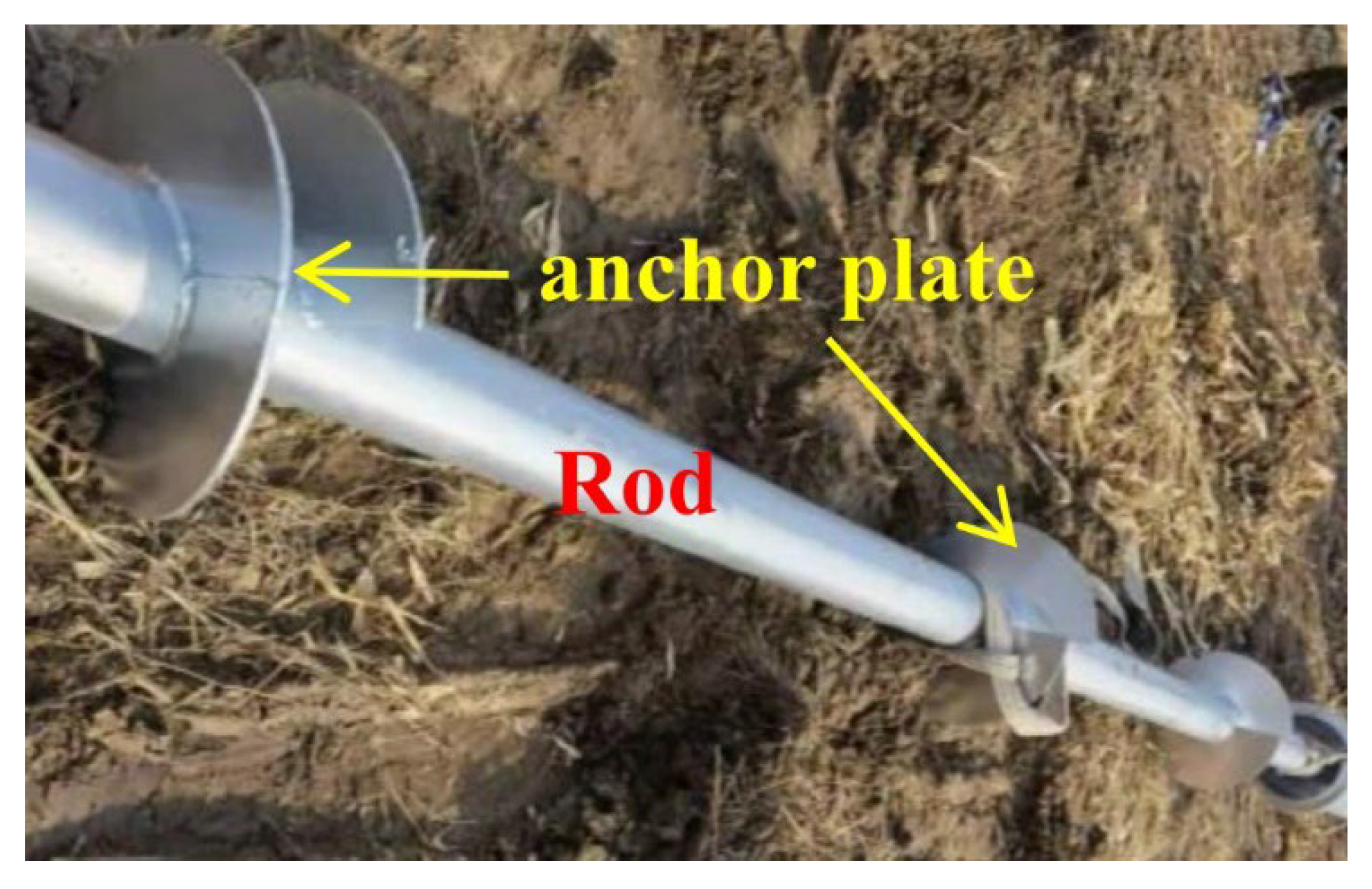
As shown in Figure 1, during helical anchor reinforcement of dam foundations, multiple anchor plates are welded onto anchor rods. These anchor plates collectively bear the uplift and downward pressure loads acting on the top of the anchor rod. The diameter of conventional helical anchor rods usually ranges from 73 mm to 965 mm, and the diameter of the anchor plates ranges from 152 mm to 1219 mm [10]. However, larger helical anchors are widely used in Japan (e.g., TSUBASA, NS-ECO, steel helical piles, and SRP) and the diameters of these anchor rods can reach 100 mm to 1600 mm [11]. The uplift bearing capacity of traditional helical anchors in dense sand soil is about 600 kN [12]. For the case of the large helical anchors used in Japan, with anchor rod diameters ranging from 800 mm to 1200 mm, the bearing capacity can reach up to 40,000 kN [13].

It is noteworthy that this helical anchor technology, with its significant engineering advantages, is not a recent innovation. The historical application of helical anchor can be traced back to 1833, when they were first used as a lighthouse foundation for tidal inland bays in Britain. Although helical anchor technology has a long history, its excellent engineering characteristics show significant application potential in modern civil engineering. In recent years, some exploratory applications of helical anchor technology have been carried out in China’s infrastructure projects.

Since 2000, helical anchor technology has been applied to the foundation engineering of transmission towers in China, and some small helical anchors have been applied in the field of coal roadway support. For example, from 2002 to 2005, the State Grid Liaoning Electric Power Co., Ltd. (Shenyang, China) applied helical anchor foundation in several projects, including the 66 kV Xinshi Line, 220 kV Dianshu Line, 220 kV Beitai 2# Line, 220 kV Taixin Line, and 220 kV Qingshu Line. In 2017, the Zibo Qilin Electric Power Design Institute Co., Ltd. (Zibo, China) adopted a helical anchor foundation for the three-base double-circuit tangent tower in the power supply project of the Jiqing High-Speed Railway Zhutai Traction Substation. In 2019, Henan Electric Power Survey & Design Institute (Zhengzhou, China) used helical group anchors in the 500 kV outgoing project of the Henan Zhumadian 1000 kV Ultra High Voltage Substation [14,15].

However, it is important to note that there is still a lack of understanding of this kind of helical piles. The existing design methods for predicting pullout resistance were not accurate, and torque evaluation models were not generally effective, because they depended on soil characteristics (which can change during the installation process) and the geometric properties of the piles, as mentioned by Merifield [16]. Further research and refinement of design methods are needed to improve the accuracy and reliability of predicting the pullout resistance of helical anchor. Huang et al. [17] explored the stress mechanism of helical anchors in the gravel soil of the Qinghai–Tibet Plateau and expanded the application range of the helical anchor foundation. With the release of specific design specifications, such as the code for the design of helical anchor foundations of overhead transmission lines (Q/GDW 10584-2022) [18] and the code for the design of foundations of overhead transmission lines (DL/T 5219-2023) [19], a theoretical basis was provided for the refined design of helical anchor foundations. In the specifications, the design formulas for the uplift and compression bearing capacity of helical anchors and the strength of anchor rods and welding seams are given in detail, but the design of the anchor plates of helical anchors is not explained. Nevertheless, the anchor plate is the key component of the helical anchor, providing the uplift and compression bearing capacity, and the failure of the anchor plate directly affects the reliability of the helical anchor.

In in situ tests, it is difficult to measure the internal forces and deformations of the anchor rod and helical plate in helical anchor foundations under uplift loading, and it is also hard to quantify the contribution of the side friction resistance provided by the surrounding soil on the uplift capacity. To investigate the mechanical behavior of helical anchor foundations and the deformation characteristics of surrounding soil, this study performs numerical analysis of the helical plate based on the results of the previous helical anchor test. The failure modes and influencing factors of helical plate are investigated, and a theoretical model of internal force and deformation calculation is established by analyzing the failure patterns of the helical plate. This model overcomes the limitation of the missing design basis in existing codes, thus providing references for the engineering design of helical anchors.

2. Analysis of Mechanical Performance of Helical Anchor Plates

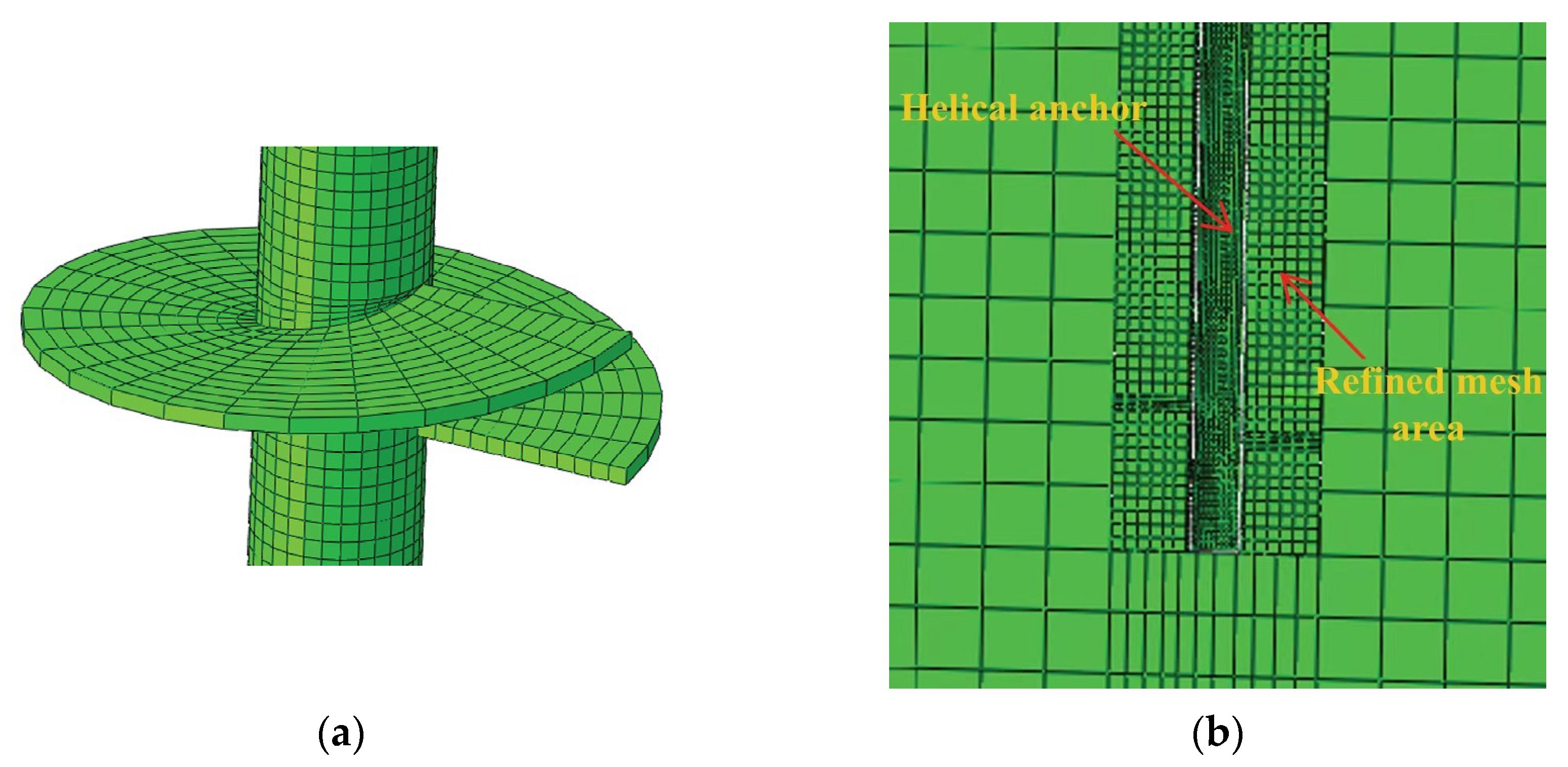
Based on the results of the previous helical anchor test, the soil quality of the test site was relatively uniform, and the soil was mainly silty clay, which was plastic to hard plastic and had medium compressibility. The numerical model of the helical anchor was established using ABAQUS R2018x finite element software, and the soil adopted a linear elastic combined Mohr–Coulomb elastoplastic model. The detailed parameters are given elsewhere [14,15]. The constitutive relation of the helical anchor’s steel material adopted an ideal elastoplastic model, and the yield strength was 345 MPa. As shown in Figure 2, when meshing the connection area between the helical plate and anchor rod, the anchor rod wall must first be sectioned along helical paths. The mesh size of the soil within one helix diameter around the helical anchor is consistent with the mesh size of the anchor rod.

In order to minimize the influence of the boundary constraints of the numerical model on the computational results, a cylindrical soil model with a diameter of 10 times the diameter of the helical anchor plate was built, and the height of cylinder was 2 times that of the embedded depth of the helical anchor. Three constraints of U_x, U_y, and U_z were applied on the bottom of the soil model, and two constraints of U_x and U_y were applied on the side of the soil model. The surface-to-surface contact condition was established between the helical anchor and the soil and the friction coefficient was 0.14. To minimize boundary effects on calculation results, the soil model boundaries maintain a clear distance of at least 10 times the helix diameter from the nearest helical plate edge. The thickness of the soil model is set to twice the embedded depth of the helical anchor.

To accurately simulate the stress distribution of the helical anchor in soil, an initial analysis of the geostress balance of the numerical model was conducted by importing initial stresses, considering the significant vertical compression deformation caused by gravity. However, the relative slip of the interface between soil and anchor rod was large, which may lead to difficulties in calculation convergence during the analysis. Therefore, it is recommended that the contact surface should not be activated in the calculation of geostress balance to obtain the initial geostress field quickly and accurately. After the first analysis, the contact surface was activated, and then one or two further analyses of geostress balance were performed. It should be noted that the numerical model was based on the final installed state of the helical anchor and cannot replicate the compression exerted by the anchor rod on the surrounding soil during the installation. Consequently, the friction between the anchor rod and the surrounding soil may be negligible, with a significant impact on the analytical results for the helical anchor rod. To address this limitation, it is necessary to account for the squeezing effect on the surrounding soil in the process of the helical anchor drilling into the soil. After the completion of the geostress balance analysis, the contact surface between the helical anchor and the soil was activated. Due to the absence of initial compressive stress between the soil and anchor rod, the side friction resistance was not obvious in the analytical process. In order to realistically simulate the mechanical behavior of helical anchor foundations in soil, through the analysis of interference between the helical anchor and the soil contact surface, the squeezing effect of the anchor rod on the soil was realized, and the radius of the anchor rod was taken as the interference fit. Subsequently, the obtained soil stress data were reintroduced incorporated into the numerical model to realize the self-balance of the soil and the extrusion of the soil by the helical anchor rod. On this basis, a further force analysis of the helical anchor was carried out.

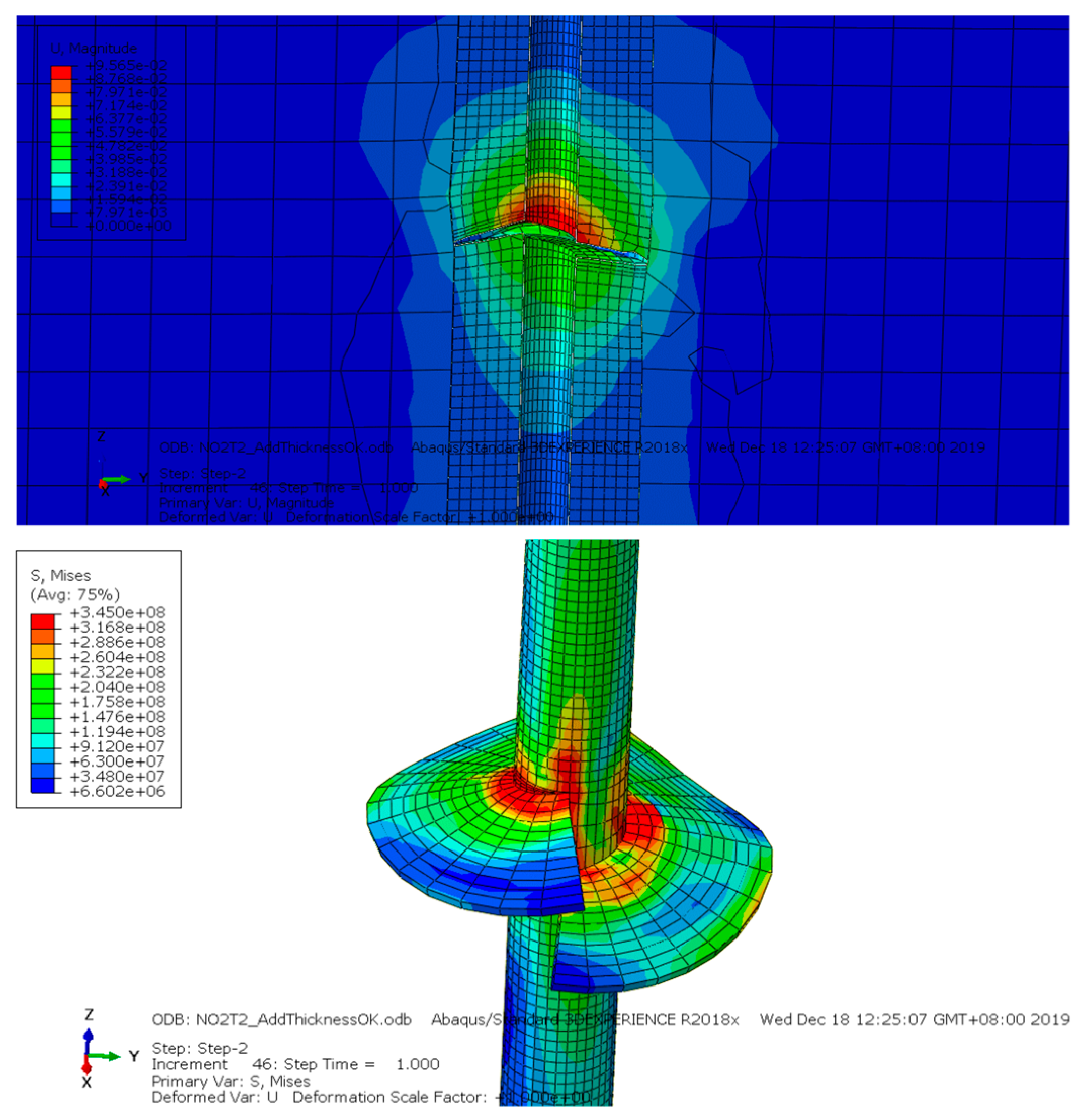
The load-displacement curve obtained via the basic numerical analysis of the helical anchor was compared with the test results, and the accuracy of the finite element model was verified. Under the action of uplift and compression load, the deformation reached 100 mm; the deformation modes of the soil and anchor plate are shown in Figure 3 and Figure 4. Notably, these figures indicate that the helical anchor plate bent obviously.

With the increase in the diameter of the helical anchor plate, the bending phenomenon of the anchor plate becomes more obvious. Additionally, the helical anchor pitch is a primary factor affecting the shape of the anchor plate. According to the requirements of the specification, the helical anchor pitch should be within the range of 1/6 to 1/3 of the diameter of the anchor plate, and the helical pitch coefficient (K_j), which is defined as the ratio of the helix diameter (D) to the axial pitch distance (p), ranges from 3 to 6. In this study, the finite element parameter analysis of the anchor plate under different helical pitches and loads is shown in Figure 5 and Figure 6.

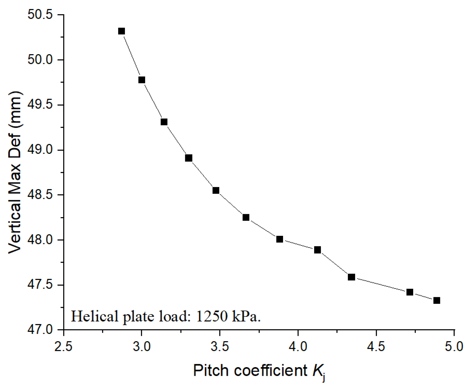
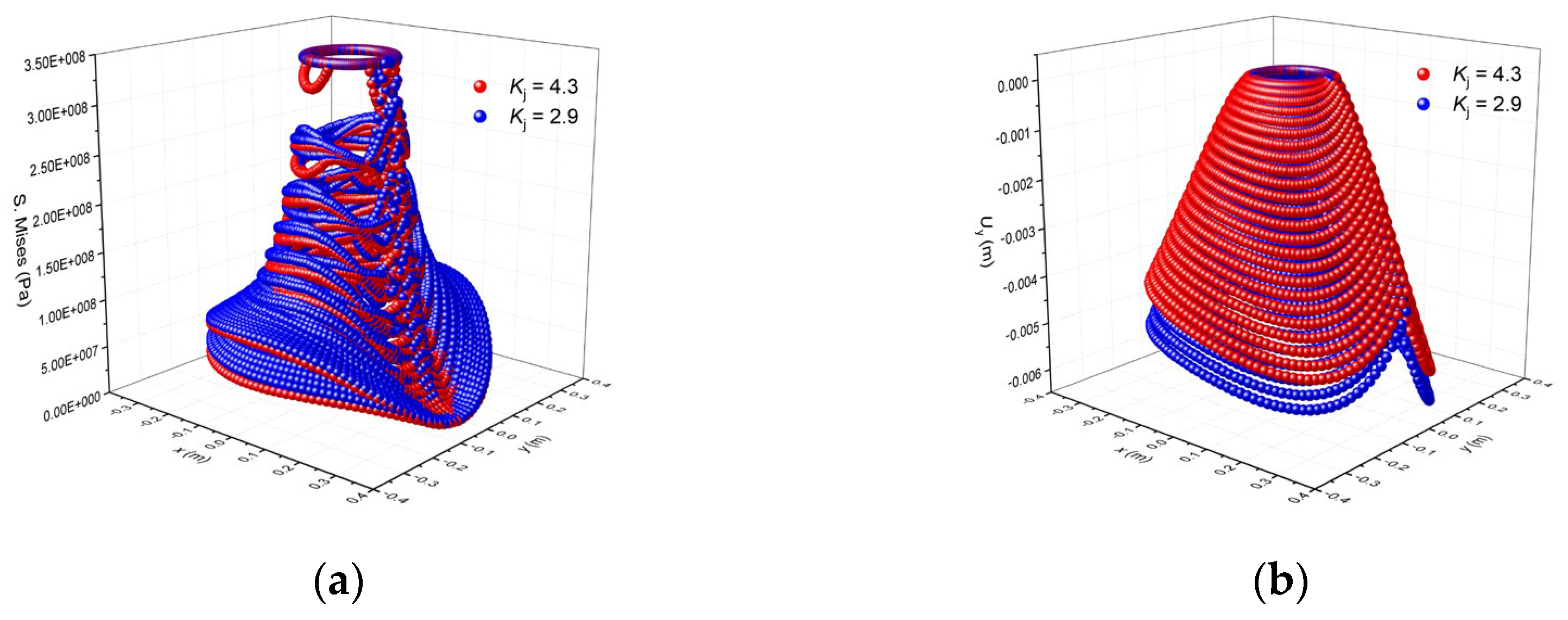
Under the condition of working load, a localized plastic region began to appear at the connection between the anchor plate and the anchor rod. With the increase in the helical pitch coefficient, the axial pitch distance decreased gradually, and the maximum vertical deformation of the anchor plate showed a decreasing trend initially, followed by an increasing trend, but the overall change was not significant.

Under the condition of ultimate load, a large plastic region appeared in the anchor plate. With the increase in the helical pitch coefficient, the maximum vertical deformation of the anchor plate decreased gradually with the decrease in the helical pitch. However, the amplitude of this decrease was approximately 6%.

As shown in Figure 7, the stress and deformation of anchor plates with different helical pitches under working load were compared. When the pitch coefficient was 2.9 and 4.3, the stress and deformation characteristics of the two anchor plates were similar. Thus, the helical pitch had little effect on the load distribution of the anchor plate.

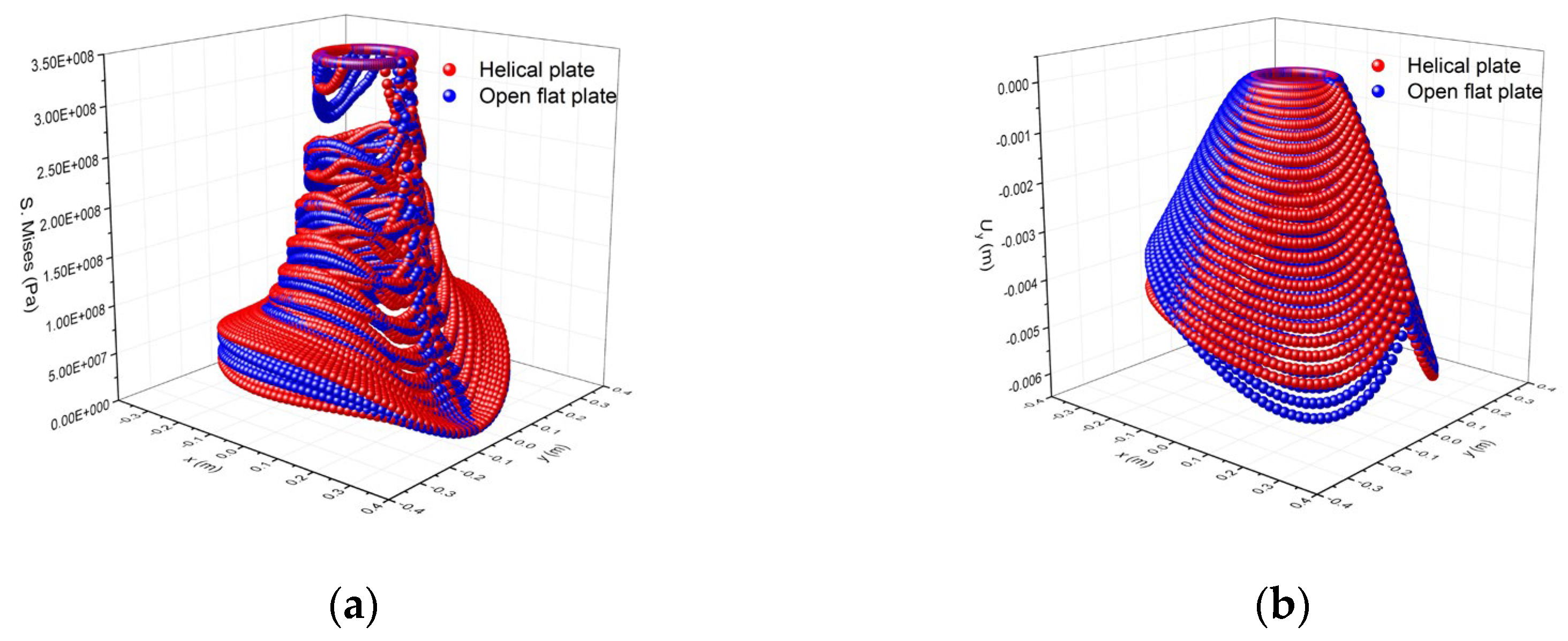
Considering that the helical pitch had little impact on the mechanical properties of the anchor plate, the helical anchor plate can be simplified to a flat circular disk, as shown in Figure 8. According to the degree of simplification, the flat circular disk can be further divided into two types: a closed circular disk and an open circular disk. Of these two types, the deformation of the open circular disk was closer to that of the helical disk.

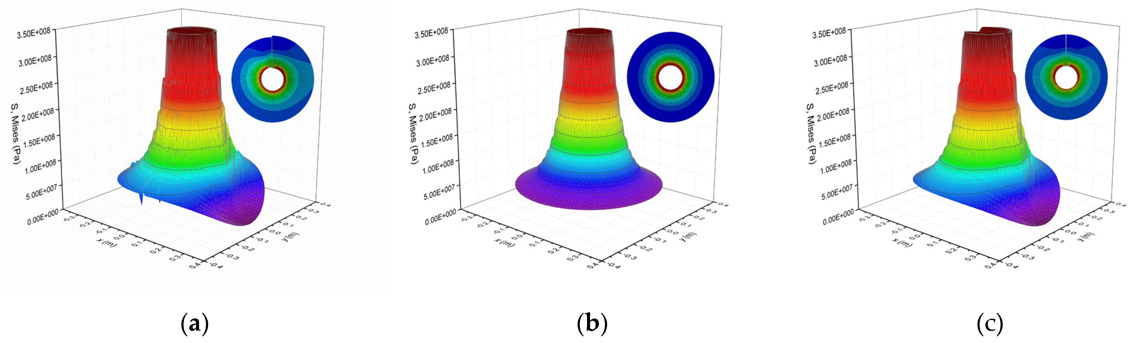
As shown in Figure 9, the stress distributions of the three kinds of plates under working loads were compared. All three kinds of plates reached the yield strength at the connection with the anchor rod (red in the diagram), and the stress decreased gradually with the increase in the distance from the anchor rod. At the disconnection site of the helical disk and the open circular disk, the stress reached 0.

3. Calculation Model

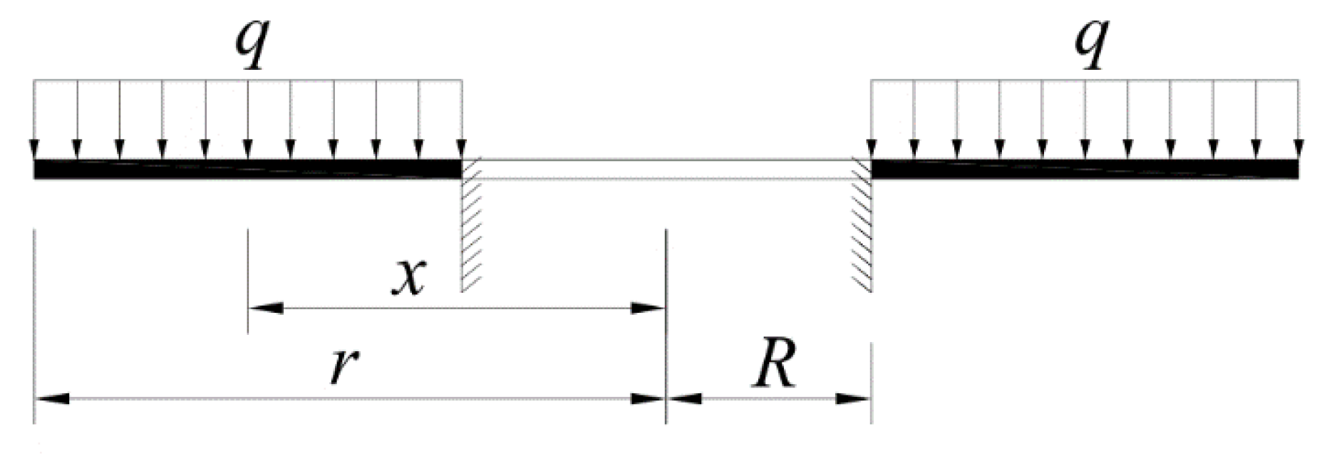
3.1. Cantilever Open Ring Disk Model

The cantilever open circular disk was composed of two concentric circles with $r=a$ and $r=b$ and two radii forming a central angle of ${\theta }_0$, as shown in Figure 10 [20]. $r=a$ was the fixed edge, and the other three sides were free edges. The load on the circular disk surface was loaded by $q$, and the concentrated force $P_1$ was acted on at $r=b$, $\theta ={\theta }_{\mathrm{l}}$ ($0<{\theta }_{\mathrm{l}}<{\theta }_0$).

According to the thin plate theory, the basic differential equations of the polar coordinate form for the small deflection problem of a flat plate are as follows:

$${\nabla }^2{\nabla }^2\omega ={\displaystyle \frac{q}{D}}$$

(1)

where ${\nabla }^2={\displaystyle \frac{{\partial }^2}{\partial r^2}}+{\displaystyle \frac{1}{r}}{\displaystyle \frac{\partial }{\partial r}}+{\displaystyle \frac{1}{r^2}}{\displaystyle \frac{{\partial }^2}{\partial {\theta }^2}}$.

According to the force of the anchor plate, the boundary conditions of the calculation model are as follows:

• $r=a$, $\omega =0$, ${\displaystyle \frac{\partial \omega }{\partial r}}=0$;
• $r=b$, $M_r=0$, $V_r=P_1\delta (\theta -{\theta }_1)$;
• $\mathsf{\theta }=0$, $M_{\theta }=0$, $V_{\theta }=0$;
• $\mathsf{\theta }={\theta }_0$, $M_{\theta }=0$, $V_{\theta }=0$;
• $r=b$, $\theta =0$, $R=0$;
• $r=b$, $\theta ={\theta }_0$, $R=0$.

In the equations above, $\omega$ is deflection, $M_r$ and $M_{\theta }$ are bending moment, $M_{r\theta }$ and $M_{\theta r}$ are torque, $Q_r$ and $Q_{\theta }$ are transverse shear, $V_r$ and $V_{\theta }$ are Kirchhoff’s generalized shear force, $R$ is corner reaction force, $v$ is Poisson’s ratio, and $D$ is bending stiffness.

Then, the deflection $\omega$ is decomposed. The assumption is:

$$\omega ={\omega }_H+{\omega }_P$$

(2)

where ${\omega }_H$ is the homogeneous solution of (1), and ${\omega }_P$ is an arbitrary particular solution.

The particular solution ${\omega }_P$ can be obtained according to the in-plane load, for the uniformly distributed load $q=q_0$:

$${\omega }_P={\displaystyle \frac{q_0{r}^4}{64D}}$$

(3)

Substitute (2) into (1):

$${\nabla }^2{\nabla }^2{\omega }_H=0$$

(4)

In order to obtain the general expression of ${\omega }_H$, a function $M(r,\theta )$ is introduced here:

$$M={\displaystyle \frac{M_r+M_{\theta }}{1+v}}=-D{\nabla }^2{\omega }_H$$

(5)

Substitute (5) into (4):

$${\nabla }^{2}M=0$$

(6)

In the following, the general expression of deflection $\omega$ is derived in two steps using curvilinear coordinate transformation.

3.1.1. The General Expression for the Function M

Let $r={\mathrm{e}}^t$ and substitute it into (6):

$${\mathrm{e}}^{-2t}\left({\displaystyle \frac{{\partial }^{2}M}{\partial t^2}}+{\displaystyle \frac{{\partial }^{2}M}{\partial {\theta }^2}}\right)=0$$

(7)

Therefore:

$${\displaystyle \frac{{\partial }^{2}M}{\partial t^2}}+{\displaystyle \frac{{\partial }^{2}M}{\partial {\theta }^2}}=0$$

(8)

The form of the solution is:

$$M=\sum _{m=1}^{\mathrm{\infty }}{T}_m\left(t\right)sin{\lambda }_m\mathsf{\theta }+\sum _{n=1}^{\mathrm{\infty }}{\theta }_n\left(\theta \right)sin{\lambda }_n\left(\mathrm{t}-lna\right)$$

(9)

where ${\lambda }_m={\displaystyle \frac{m\pi }{{\theta }_0}}$ and ${\lambda }_n={\displaystyle \frac{n\pi }{ln\frac{b}{a}}}$.

From (8), it can be deduced that:

$$T_m\left(t\right)=A_m^{\prime }{\mathrm{e}}^{\lambda mt}+B_m^{\prime }{\mathrm{e}}^{-\lambda mt}$$

(10)

$${\theta }_n\left(\theta \right)=A_n^{\prime }ch{\lambda }_n\theta +B_n^{\prime }sh{\lambda }_n\theta$$

(11)

where $A_m^{\prime }$, $B_m^{\prime }$, $A_n^{\prime }$ and $B_n^{\prime }$ are constants of integration.

3.1.2. Derive the General Solution of ${\omega }_H$

The general solution for $M$ has already been obtained above. Now, based on $M$, the general solution for ${\omega }_H$ is obtained. Based on (5):

$${\displaystyle \frac{{\partial }^2{\omega }_H}{\partial r^2}}+{\displaystyle \frac{1}{r}}{\displaystyle \frac{\partial {\omega }_H}{\partial r}}+{\displaystyle \frac{1}{r^2}}{\displaystyle \frac{{\partial }^2{\omega }_H}{\partial {\theta }^2}}=-{\displaystyle \frac{M}{D}}$$

(12)

Let $r={\mathrm{e}}^t$. Thus, (12) can be transformed into:

$${\displaystyle \frac{{\partial }^2\omega }{\partial t^2}}+{\displaystyle \frac{{\partial }^2\omega }{\partial {\theta }^2}}=-{\displaystyle \frac{1}{D}}\left\{\begin{array}{c}{\displaystyle \sum _{m=1}^{\mathrm{\infty }}}\left. [A_m^{\prime }{\mathrm{e}}^{{(\lambda }_m+2)t}+B_m^{\prime }{\mathrm{e}}^{\left(2-{\lambda }_m\right)t}\right]sin{\lambda }_m\theta +\\ {\displaystyle \sum _{n=1}^{\mathrm{\infty }}}(A_m^{\prime }ch{\lambda }_n\theta +B_n^{\prime }sh{\lambda }_n\theta )e^{2t}sin{\lambda }_n(t-lna)\end{array}\right\}$$

(13)

Solving (13) yields:

$$\begin{array}{cc}\hfill {\omega }_H& =K_1{e}^{t}cos\theta +K_2{e}^{t}sin\theta +{\displaystyle \sum _{m=1}^{\mathrm{\infty }}}[A_m{\mathrm{e}}^{{(\lambda }_m+2)t}+B_m{\mathrm{e}}^{\left(2-{\lambda }_m\right)t}+C_{m}ch{\lambda }_m\left(t-lna\right)\hfill \\ & +{\mathrm{D}}_{m}sin{\lambda }_m(t-lna)]sin{\lambda }_m\theta +{\displaystyle \sum _{n=1}^{\mathrm{\infty }}}\left\{\right(A_{n}ch{\lambda }_n\theta +B_{n}sh{\lambda }_n\theta ){\mathrm{e}}^{2t}[\mathrm{s}in{\lambda }_n(\mathrm{t}-lna)\hfill \\ & -{\lambda }_{n}cos{\lambda }_n\left(t-lna\right)]+({\mathrm{C}}_{n}ch{\lambda }_n\theta +{\mathrm{D}}_{n}sh{\lambda }_n\theta \left)sin{\lambda }_n\right(t-lna\left)\right\}\hfill \end{array}$$

(14)

where $A_m$, $B_m$, $C_m$, $D_m$, $A_n$, $B_n$, $C_n$, $D_n$, $K_1$ and $K_2$ are undetermined constants.

In (14), it needs to be specifically explained that the terms $e^{t}cos\theta$ and $e^{t}sin\theta$ correspond to the terms associated with rigid body rotation. The respective internal force components $M_r$, $M_{\theta }$, $M_{r\theta }$, $Q_r$ and $Q_{\theta }$ corresponding to these terms are all equal to 0.

Thus, the general expression for the deflection $\omega$ is obtained. Since $\omega$ is expressed in terms of the new coordinates $t$ and $\theta$, the boundary conditions should also be expressed using $t$ and $\theta$, which are:

• $t=lna$, $\omega =0$;
• $t=lna$, ${\displaystyle \frac{\partial \omega }{\partial t}}=0$;
• $t=lnb$, ${\displaystyle \frac{{\partial }^2\omega }{\partial t^2}}-\left(1-v\right){\displaystyle \frac{\partial \omega }{\partial t}}+v{\displaystyle \frac{{\partial }^2\omega }{\partial {\theta }^2}}=0$;
• $t=lnb$, ${\displaystyle \frac{{\partial }^3\omega }{\partial t^8}}+\left(2-v\right){\displaystyle \frac{{\partial }^3\omega }{\partial t\partial {\theta }^2}}-2{\displaystyle \frac{{\partial }^2\omega }{\partial t^2}}-\left(3-v\right){\displaystyle \frac{{\partial }^2\omega }{\partial {\theta }^2}}=-{\displaystyle \frac{2p_1{b}^2}{D{\theta }_0}}\sum _{m=1}^{\mathrm{\infty }}sin{\lambda }_m{\theta }_{1}sin{\lambda }_m\theta$;
• $\theta =0$, $v{\displaystyle \frac{{\partial }^2\omega }{\partial t^2}}+\left(1-v\right){\displaystyle \frac{\partial \omega }{\partial t}}+{\displaystyle \frac{{\partial }^2\omega }{\partial {\theta }^2}}=0$;
• $\theta ={\theta }_0$, $v{\displaystyle \frac{{\partial }^2\omega }{\partial t^2}}+\left(1-v\right){\displaystyle \frac{\partial \omega }{\partial t}}+{\displaystyle \frac{{\partial }^2\omega }{\partial {\theta }^2}}=0$;
• $\theta =0$, ${\displaystyle \frac{{\partial }^3\omega }{\partial {\theta }^3}}+\left(2-v\right){\displaystyle \frac{{\partial }^3\omega }{\partial t^2\partial \theta }}-3\left(1-v\right){\displaystyle \frac{{\partial }^2\omega }{\partial t\partial \theta }}+2\left(1-v\right){\displaystyle \frac{\partial \omega }{\partial \theta }}=0$;
• $\theta ={\theta }_0$, ${\displaystyle \frac{{\partial }^3\omega }{\partial {\theta }^3}}+\left(2-v\right){\displaystyle \frac{{\partial }^3\omega }{\partial t^2\partial \theta }}-3\left(1-v\right){\displaystyle \frac{{\partial }^2\omega }{\partial t\partial \theta }}+2\left(1-v\right){\displaystyle \frac{\partial \omega }{\partial \theta }}=0$;
• $t=lnb$, $\theta =0{\displaystyle \frac{{\partial }^2\omega }{\partial t\partial \theta }}-{\displaystyle \frac{\partial \omega }{\partial \theta }}=0$
• $t=lnb$, $\theta ={\theta }_0{\displaystyle \frac{{\partial }^2\omega }{\partial t\partial \theta }}-{\displaystyle \frac{\partial \omega }{\partial \theta }}=$0.

By combining the aforementioned 10 sets of infinite equations, the undetermined constants $A_m$, $B_m$, $C_m$, $D_m$, $A_n$, $B_n$, $C_n$, $D_n$, $K_1$ and $K_2$ can be determined.

3.2. Cantilever Closed Ring Disk Model

The calculation model of the cantilever closed ring disk is shown in Figure 11. The corresponding deformation and internal force calculation formulas can be obtained from the Static Calculation Handbook for Practical Structure [21].

$$\begin{array}{cc}\hfill f& ={\displaystyle \frac{q{R}^4}{64D}}\left\{-1\right.+2 [1-2{\beta }^2-{\displaystyle \frac{\left(1-v\right){\beta }^2+(1+v)(1+4{\beta }^{2}ln\beta )}{1-v+\left(1+v\right){\beta }^2}}\left.{\beta }^2\right]\left(1-{\rho }^2\right)\hfill \\ & +{\rho }^4-4{\displaystyle \frac{\left(1-v\right){\beta }^2+(1+v)(1+4{\beta }^{2}ln\beta )}{1-v+\left(1+v\right){\beta }^2}}{\beta }^{2}ln\rho -8{\beta }^2{\rho }^2\left.ln\rho \right\}\hfill \end{array}$$

(15)

$$\begin{array}{cc}\hfill M_r& ={\displaystyle \frac{q{R}^2}{16}}\left\{4{\beta }^2\right.+\left(1+v\right) [1-{\displaystyle \frac{\left(1-v\right){\beta }^2+(1+v)(1+4{\beta }^{2}ln\beta )}{1-v+\left(1+v\right){\beta }^2}}\left.{\beta }^2\right]-\left(3+v\right){\rho }^2\hfill \\ & -{\displaystyle \frac{1-v}{{\rho }^2}}\cdot {\displaystyle \frac{\left(1-v\right){\beta }^2+(1+v)(1+4{\beta }^{2}ln\beta )}{1-v+\left(1+v\right){\beta }^2}}{\beta }^2+4(1+v){\beta }^2\left.ln\rho \right\}\hfill \end{array}$$

(16)

$$\begin{array}{cc}\hfill M_t& ={\displaystyle \frac{q{R}^2}{16}}\left\{4v{\beta }^2\right.+\left(1+v\right) [1-{\displaystyle \frac{\left(1-v\right){\beta }^2+(1+v)(1+4{\beta }^{2}ln\beta )}{1-v+\left(1+v\right){\beta }^2}}\left.{\beta }^2\right]-\left(1+3v\right){\rho }^2\hfill \\ & +{\displaystyle \frac{1-v}{{\rho }^2}}\cdot {\displaystyle \frac{\left(1-v\right){\beta }^2+(1+v)(1+4{\beta }^{2}ln\beta )}{1-v+\left(1+v\right){\beta }^2}}{\beta }^2+4(1+v){\beta }^2\left.ln\rho \right\}\hfill \end{array}$$

(17)

$$V_r=-{\displaystyle \frac{qR}{2}}(\rho -{\displaystyle \frac{{\beta }^2}{\rho }})$$

(18)

In (15) to (18), $q$ is the axisymmetric ring’s uniformly distributed load, $M_r$ is the radial bending moment, $M_t$ is the tangential bending moment, $V_r$ is the shear force, $f$ is the deflection, $D={\displaystyle \frac{E{t}^3}{12(1-v^2)}}$ is the stiffness of the plate, $E$ is the elastic modulus, $v$ is the Poisson’s ratio, $\rho ={\displaystyle \frac{x}{R}}$ and $\beta ={\displaystyle \frac{r}{R}}$. The bending moment causes compression on the upper part of the plate and tension on the lower part, with positive values. The downward deflection is considered positive. The shear force is positive when it acts counterclockwise with respect to the normal of the cross-section.

3.3. Determination of the Calculation Method

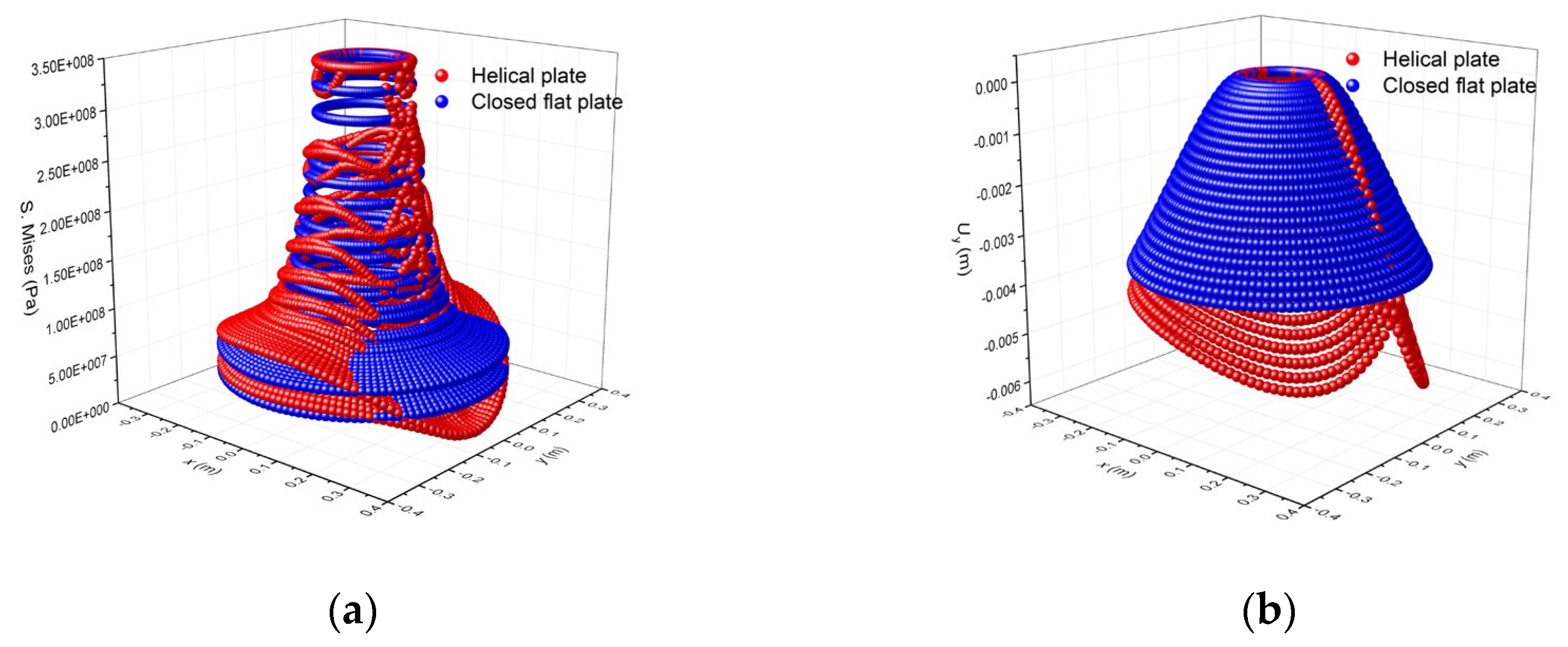
A comparison of the above theoretical calculation results and the numerical analysis of the helical disk is shown in Figure 12 and Figure 13. The stress distribution of the closed flat disk (Figure 12) and the open flat disk (Figure 13) demonstrates significant consistency with that of the whole helical disk, particularly at the connection between the disk and the anchor rod, exhibiting an ideal match. Comparatively, the maximum deformation of the closed flat disk is slight smaller than that of the helical disk, and the difference is not more than 3 mm. Conversely, the deformation of the open flat disk closely approximates that of the helical disk.

Consequently, both the theoretical calculation models and the numerical analysis models provide accurate predictions for the internal force and deformations of the helical disk under surface loading. However, the formula related to the closed circular disk provides a simpler and more convenient method for practical design purposes.

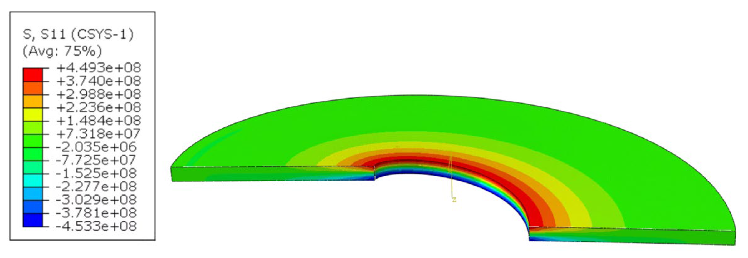
3.3.1. Comparison of Results for a Closed Flat Disk

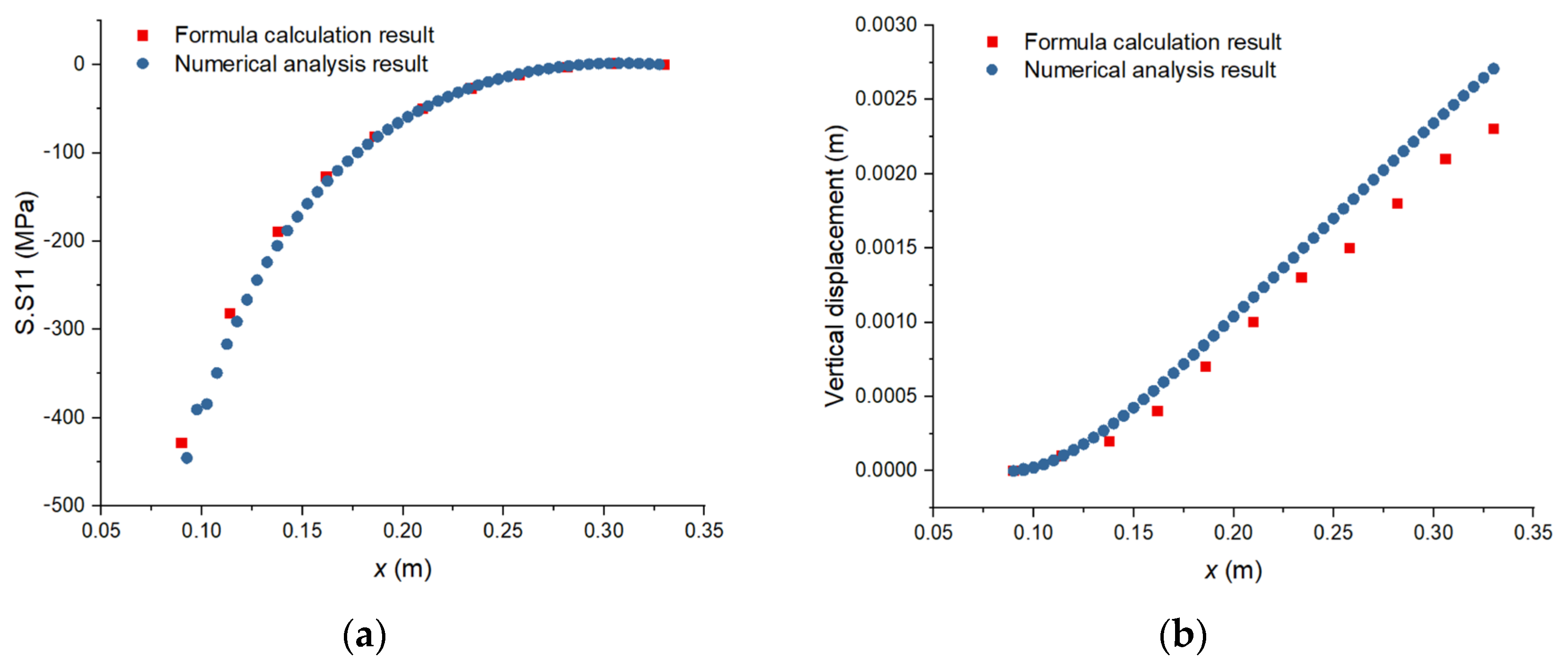
To verify the accuracy of the theoretical formula, the numerical analysis models used in the following analysis do not account for steel yielding. By comparing the formula calculation results of the closed flat disk with the numerical analysis results of the helical disk, the connection between the circular disk and the anchor rod is treated as an unfolded rectangular beam.

Utilizing (16), the bending moment can be determined; subsequently, the maximum stress and corresponding deformation of the circular disk under surface loading can be calculated. These results are then compared with the results of the numerical analysis, as shown in Figure 14.

As shown in Figure 15, the theoretical calculated stresses and displacements are completely consistent with the numerical analysis results, which verifies the accuracy of the theoretical formula and the rationality of unfolding the junction of the anchor plate and the anchor rod into a rectangular beam.

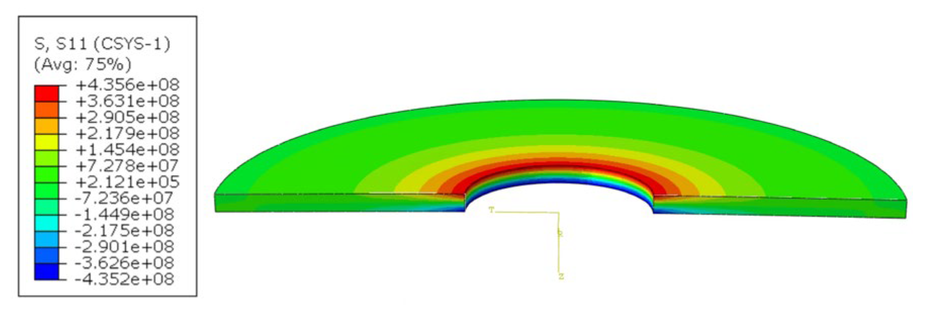
3.3.2. Comparison of a Closed Flat Disk with a Helical Disk

In contrast to the symmetrical stress distribution observed in a closed flat disk, the stress distribution in a helical disk under the surface loading exhibits asymmetry. In order to conduct a comparative analysis, a cross-section situated 90 degrees away from the opening of the helical anchor plate (the stress distribution tends to be uniform) was selected as the focal point of investigation. Figure 16 displays the stress distribution contour plot of the selected section.

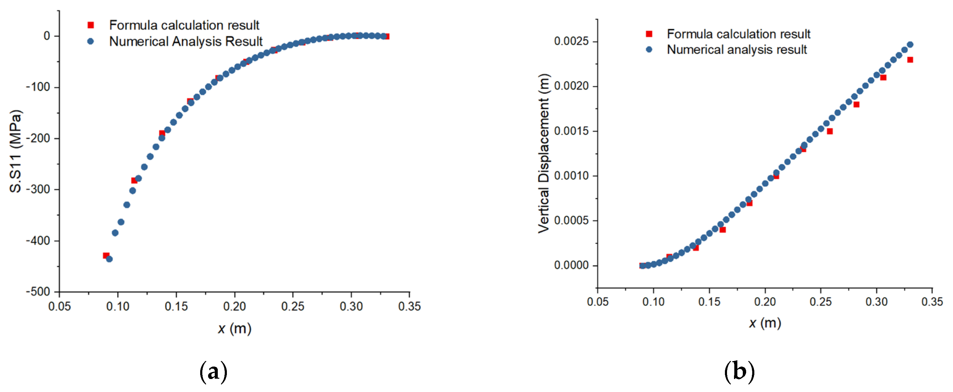
The outcomes derived from the formula for a closed flat disk are compared with the numerical analysis results for the helical disk, as shown in Figure 17. The stress values calculated using the theoretical formula are in good agreement with the numerical analysis results. However, the deformation calculated by the formula is marginally smaller than that obtained from the numerical analysis.

The formulas used for calculating the internal force and deformation of the closed flat disk can effectively predict the bearing performance of the spiral plate. Furthermore, under working load conditions, the deformation of the anchor plate is relatively small, typically entering the plastic zone only in the area with higher stress, specifically at the top and bottom of the connection with the anchor rod.

Therefore, when using the above method to design the helical anchor plate, it is advisable to consider allowing for the partial plastic development of the anchor plate. Based on the calculation files of the Belo Monte Ultra-High Voltage Transmission Project in Brazil, it is suggested that the plastic development coefficient ranges from 1.2 to 1.5.

Combined with the above contents and calculation formulas, the corresponding calculation code of helical anchor plate (in MATLAB 2018 version) is provided in Appendix A for reference.

4. Conclusions

In this study, based on the in situ test results of a helical anchor used for dam foundation reinforcement, the numerical analysis of the anchor plate is carried out, and the failure mode of the anchor plate is revealed. A prediction-based theoretical model, which can evaluate the bearing capacity and deformation of the anchor plate, is established. The following key conclusions are drawn:

(1)

Under the action of uplift and compression load, when the dam foundation reinforced with a helical anchor reaches a large deformation, the anchor plate may bend obviously.

(2)

The influence of the pitch on the mechanical performance of the anchor plate is not obvious, and the helical anchor plate can be simplified into a flat circular disk. It is worth nothing that the deformation of the open circular disk is similar to that of the helical disk. Additionally, at the disconnection site of the helical disk and the open circular disk, the stress is 0.

(3)

The stress distribution of the closed flat disk and the open flat disk is in good agreement with that of the whole helical disk, particularly at the connection between the disk and the anchor rod. The maximum deformation of the closed flat disk is slightly smaller than that of the helical disk (about 6%). The deformation of the open flat disk is in good agreement with that of the helical disk. Both the theoretical calculation model and the numerical analysis model provide accurate predictions for the internal force and deformation of the helical disk under surface loading. However, the formula related to the closed flat disk provides a simpler and more convenient method for practical design and application. Notably, the deformation of the anchor plate is relatively small under working loads. When large loads lead to significant deformation, a modification is carried out in combination with plastic development.