Study on the Distribution Characteristics of Thermal Melt Geological Hazards in Qinghai Based on Remote Sensing Interpretation Method

Abstract

In recent years, large-scale linear infrastructure developments have been developed across hundreds of kilometers of permafrost regions on the Qinghai–Tibet Plateau. The implementation of major engineering projects, including the Qinghai–Tibet Highway, oil pipelines, communication cables, and the Qinghai–Tibet Railway, has spurred intensified research into permafrost dynamics. Climate warming has accelerated permafrost degradation, leading to a range of geological hazards, most notably widespread thermokarst landslides. This study investigates the spatiotemporal distribution patterns and influencing factors of thermokarst landslides in Qinghai Province through an integrated approach combining field surveys, remote sensing interpretation, and statistical analysis. The study utilized multi-source datasets, including Landsat-8 imagery, Google Earth, GF-1, and ZY-3 satellite data, supplemented by meteorological records and geospatial information. The remote sensing interpretation identified 1208 cryogenic hazards in Qinghai’s permafrost regions, comprising 273 coarse-grained soil landslides, 346 fine-grained soil landslides, 146 thermokarst slope failures, 440 gelifluction flows, and 3 frost mounds. Spatial analysis revealed clusters of hazards in Zhiduo, Qilian, and Qumalai counties, with the Yangtze River Basin and Qilian Mountains showing the highest hazard density. Most hazards occur in seasonally frozen ground areas (3500–3900 m and 4300–4900 m elevation ranges), predominantly on north and northwest-facing slopes with gradients of 10–20°. Notably, hazard frequency decreases with increasing permafrost stability. These findings provide critical insights for the sustainable development of cold-region infrastructure, environmental protection, and hazard mitigation strategies in alpine engineering projects.

1. Introduction

Permafrost, a critical component of the cryosphere, refers to lithospheric materials (rocks and soils) containing ice that persist at or below 0 °C for extended periods. Depending on the duration of the frozen state, it is classified into three categories: (1) short-term frozen ground (hours to two weeks), (2) seasonally frozen ground (half-month to <1 year, undergoing annual freeze–thaw cycles), and (3) permafrost (≥2 years to millennia) [1,2,3]. Permafrost covers approximately 24% of the Earth’s terrestrial surface, primarily distributed in Northern Hemisphere high-latitude zones (covering > 50% of Russia and Canada, 85% of Alaska) and mid-latitude alpine regions (22% of China’s territory), along with Antarctic peripheries [4]. As the world’s third-largest permafrost repository, China contains approximately 2.15 million km² of permafrost (≈10% global share, 22.4% national land area), predominantly distributed across the Qinghai–Tibet Plateau, Greater and Lesser Khingan Mountains, Altai–Tianshan ranges, Qilian Mountains, and Bayan Har Mountains [2]. Notably, China’s mountain permafrost accounts for >60% of global alpine permafrost and 92% of national permafrost coverage [5]. The Qinghai–Tibet Plateau (28–37° N, 75–103° E), with an average elevation exceeding 4000 m (central plateau > 4500 m), represents the largest mid-latitude permafrost zone globally. Its distinctive cryospheric regime—sustained by mean annual temperatures of −7.0 °C to −3.0 °C and extreme altitude—preserves the world’s most extensive high-elevation permafrost [6]. In contrast to its high-latitude counterparts, this plateau permafrost exhibits unique thermal characteristics: higher baseline temperatures (−1.5 °C to −3.5 °C), thinner active layers (1–4 m), and pronounced spatial heterogeneity in ground thermal regimes.

The intensification of global warming coupled with socioeconomic development has driven increased anthropogenic engineering interventions across permafrost regions, triggering widespread thermokarst landslides. In China, these thermokarst landslides have been systematically documented on the Qinghai–Tibet Plateau [7,8,9], Tianshan Mountains [10], Qilian Mountains [11], and Greater/Lesser Khingan Mountains [12]. Comparable phenomena are observed globally in ice-rich permafrost zones: Arctic Canada [13,14], Alaska [15,16], and Siberian Russia [17]. As one of the most visible manifestations of permafrost degradation, thermokarst landslides, through thermal erosion processes, have profound environmental and infrastructural consequences. Their cascading effects—including terrain destabilization, carbon release, and infrastructure damage—have elevated this phenomenon to a critical research frontier in permafrost science.

The extensive deployment of linear infrastructure projects (e.g., Qinghai–Tibet Highway, oil pipelines, fiber-optic networks, Qinghai–Tibet Railway) across hundreds of kilometers of permafrost regions on the Qinghai–Tibet Plateau has led to substantial advancements in permafrost research. While borehole drilling and ground temperature monitoring remain the most direct methods for confirming permafrost presence, their implementation faces substantial challenges in extreme high-altitude environments. Remote sensing has become a key tool for mapping permafrost distribution, classifying types, delineating boundaries, and estimating thickness. Technological advancements—including reduced costs of high-resolution imagery (<1 m/pixel), enhanced temporal coverage of moderate-resolution datasets (e.g., Landsat time series), and improved image processing algorithms—have revolutionized thermokarst monitoring. Modern techniques now allow for detailed analysis of coastal morphology changes, thawing peatland subsidence ranging from 2 to 8 cm per year, and retrogressive thaw slumps (RTS) through integrated approaches combining multi-spectral analysis and digital elevation modeling [18,19,20]. Cutting-edge technologies such as SAR and airborne LiDAR offer unparalleled potential demonstrating exceptional capabilities in permafrost studies, particularly for detecting centimeter-scale surface deformations (InSAR precision: ±3 mm) and 3D terrain reconstruction (LiDAR vertical accuracy: <15 cm). However, the prohibitive costs of airborne LiDAR (>USD 500/km²) currently limit its application to localized corridor surveys or critical engineering sections [21,22]. Comparatively, high-resolution optical imagery (WorldView-3: 0.31 m) coupled with historical aerial photographs provides a cost-effective solution (≈1/10 LiDAR costs) for large-area thermokarst mapping, achieving classification accuracies exceeding 85% in plateau environments, as validated by previous benchmark studies in plateau environments. Hyperspectral and LiDAR can significantly enhance recognition from the following dimensions: (1) Hyperspectral (400–2500 nm, >200 band) can capture the subtle spectral absorption characteristics of mineral weathering, water content, and vegetation stress on the surface of frost mounds (such as the ‘red edge’ displacement of moss at 680–720 nm). Using spectral angle matching (SAM) or a deep learning spatial–spectral fusion network, the classification accuracy is improved from 72% of sub-meter images to >90%. (2) The lidar provides a point cloud with a vertical accuracy of <0.1 m, and the micro-terrain uplift of more than 0.2 m is directly extracted by the difference between the digital terrain model (DTM) and the digital surface model (DSM). At the same time, the intensity information can distinguish the difference between moss–bare soil coverage, and realize the centimeter-level mapping of the three-dimensional morphology and distribution of frost mounds; here, the missed detection rate is reduced to <5%.

Numerous studies have examined the characteristics and evolution of thermokarst lakes through remote sensing techniques. Jones et al. [23] utilized 1950/51 black-and-white aerial photographs, 1978 color infrared photographs, and 2006–2007 IKONOS satellite imagery to quantitatively analyze thermokarst lake changes on the northern Seward Peninsula, Alaska, revealing a paradoxical trend: an increased lake count alongside a reduction in total surface area. Carroll et al. [24] employed moderate-resolution MODIS data to report a substantial net loss of over 6700 km² in lake coverage in Canadian Arctic lake coverage between 2000 and 2009. Luo et al. [25] explored the temporal evolution of thermokarst lakes in the Beiluhe Basin using 1969 aerial photographs and 2003/2010 SPOT-5 satellite imagery, demonstrating significant increases in both lake quantity and areal extent. Research into RTS has largely focused on headwall retreat and morphological changes, integrating remote sensing and field surveys. Lantuit and Pollard [26] analyzed RTS in Yukon, Canada, using orthorectified aerial photos (1952/1970) and 2000 IKONOS images, identifying 125% and 160% increases in RTS count and total area from 1952 to 2000, with accelerated activation rates during 1970–2000. Balser et al. [27] mapped 79 RTS features near Feniak Lake, Alaska, through 2006 photogrammetry and field investigations, and highlighted their preferential formation along lake shores and riverbanks. Muste et al. [28] are conducting mapping and monitoring of thermokarst lakes in permafrost regions in the circum-Arctic and sub-Arctic permafrost regions. Lindgren et al. [29] utilized Landsat Multispectral Scanner System images from the 1970s (1972, 1974, and 1975) and Operational Land Imager images from the 2010s (2013, 2014, and 2015) to assess broad-scale distribution and changes of lakes larger than 1 ha across the four permafrost zones (continuous, discontinuous, sporadic, and isolated extent) in western Alaska. Yu et al. [30] built the first 10 m resolution Thermokarst lakes and ponds (TLP) dataset for the Lena Basin in the 2020 thawing season by utilizing 4902 Sentinel-2 images. A robust mapping workflow was developed and implemented in the Google Earth Engine (GEE) platform. The accuracy assessment demonstrates satisfactory accuracy (93.63%), and our results exhibit better consistency with real TLPs than global water body products. Shen et al. [31] proposes a method for capturing inter-annual changes of thermokarst lakes based on the “thaw–freeze” transition points and time-series SAR imagery. This method identifies the “thaw–freeze” transition points for thermokarst lakes across the entire Qinghai–Tibet Plateau, ensuring that each lake is in a similar thermal state, and proposes an improved U-net-based extraction algorithm for thermokarst lakes.

Remote sensing techniques have been extensively employed in international studies of RTS, enabling detailed time-series analysis of surface deformation. However, their application remains limited in China’s mountainous regions owing to their limited spatial extent, irregular morphologies, and discontinuous distribution of RTS. Domestic research predominantly emphasizes field investigations and laboratory simulations, with a stronger emphasis on mechanistic investigations into RTS initiation and slope instability processes over quantitative change detection. Although headwall retreat constitutes a critical component of RTS evolution, a holistic assessment requires consideration of lateral expansion dynamics and volumetric changes. Quantitative evaluation of these multidimensional dynamics is essential for evaluating environmental impacts, including estimations of soil erosion rates and assessments of carbon fluxes.

To effectively investigate the long-term dynamics of RTS, the use of high-resolution remote sensing data across multiple timeframes is essential. With the advancement of remote sensing technology, high-resolution imagery captures not only the spectral properties of surface features but also their structural composition, geometric forms, and textural attributes, thus offering enriched datasets that enable novel approaches for RTS identification and extraction. Based on this, to investigate the development process of RTS in Qinghai, this study employs historical aerial photographs and high-resolution satellite imagery as data sources. Employing object-oriented image analysis techniques, this study develops a rapid method for extracting RTS-related information. Through extracting RTS information, we analyze their spatiotemporal evolution patterns to reveal their spatial distribution characteristics, evolutionary mechanisms, and driving factors.

2. Engineering Background

Qinghai Province lies in the northern sector of the Qinghai–Tibet Plateau, an area collectively known as the ‘Roof of the World’ together with Tibet, and maintains an average elevation above 3000 m. As shown in the digital elevation model (DEM) topographic map of Qinghai Province (Figure 1), the region predominantly features elevations ranging from 4000 to 5000 m, as illustrated by the DEM topographic map. The highest point is Bukadaban Peak (6860 m), the main summit of the Kunlun Mountains along the western Qinghai–Xinjiang border, while the lowest elevation (1650 m) occurs in the Huangshui Valley at the Qinghai–Gansu boundary, creating a dramatic elevation range of approximately 5200 m. The province’s terrain exhibits pronounced topographic variation, descending progressively from west to east, with northern and southern highlands flanking a lower central basin.

Qinghai Province encompasses rich ecosystems and varied natural landscapes, with elevation gradually declining from the southwest to the northeast. The territory is traversed by multiple mountain ranges exceeding 1000 km in length from north to south, including the Qilian Mountains, Altun Mountains, Kunlun Mountains, Bayan Har Mountains, Anyemaqen Mountains, and Tanggula Mountains. Most summits rising above 5000 m remain perpetually snow-capped, boasting widespread glacial coverage. Between these mountain ranges lie plateaus, basins, and valleys.

The western mountains exhibit extreme ruggedness, gradually sloping eastward, primarily arranged in east–west and north–south orientations that form Qinghai’s topographic framework. The province’s terrain is categorized into three distinct regions, including the Qilian Mountain Region, located in the northeastern part of the province, bordering the Hexi Corridor to the north and east, and adjacent to the Qaidam Basin to the south. This area consists of a series of northwest–southeast trending fold–fault block mountains and valleys. Extending approximately 1200 km east–west and 250–400 km north–south, it covers 110,000 km², with its western and northern edges extending into Gansu Province. Average elevations exceed 4000 m, featuring prominent vertical landscape differentiation and well-developed trellis drainage patterns. A considerable number of peaks exceeding 5000 m are concentrated in the western section. Peaks and valleys above 4500 m maintain perennial snow and glaciers, with modern glaciers extensively developed. Six valleys (e.g., Heihe River Valley) run north–south, each 20–30 km wide. With the exception of the southern desert and Gobi zones, most slopes below 4200 m support lush pastureland, constituting vital natural grazing areas. The eastern section has fewer parallel ridges, lower elevations (~4000 m), with glaciers only on the Lenglong Range. Valleys (e.g., the Qinghai Lake Basin, Gonghe Basin, Xining Basin, Datong River Valley, Huangshui Valley, and Yellow River Valley) average 2500 m in elevation. Surrounding mountains (~4000 m) mostly sustain pasture except for permanently snow-capped peaks, while shaded slopes provide premium grazing land. These valleys host expansive fluvial terraces, characterized by warm and humid climates, and nutrient-rich soils that supported early agricultural development.

3. Remote Sensing Survey and Interpretation Workflow for Thermokarst Hazards in Qinghai

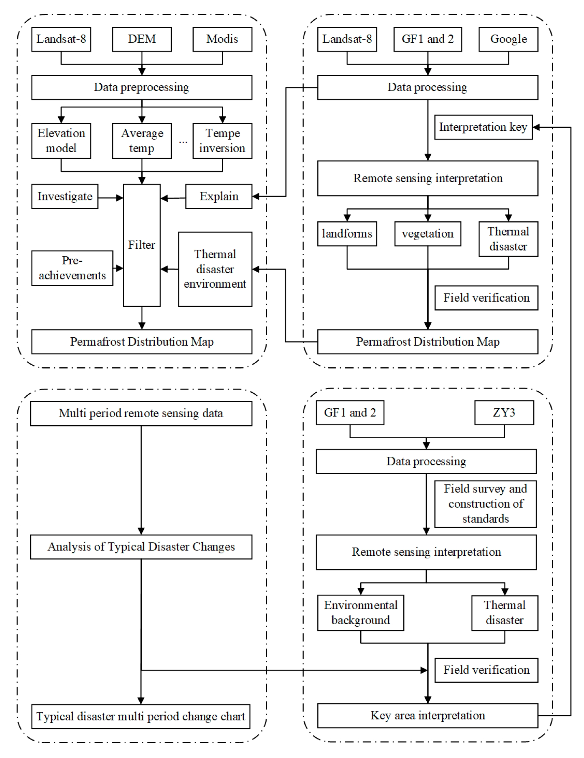
The remote sensing interpretation work commenced in June 2019 and was completed in November 2021. The methodological framework comprised the following stages: First, comprehensive collection and analysis of previous research findings were conducted. Baseline image data for the study area were acquired thereafter. Second, the integration of geospatial science (GS) and geographic information systems (GIS) technologies took place; the methodology combined remote sensing data with multi-source datasets, automated computer-based information extraction with interactive interpretation involving human expertise and digital tools, and indoor comprehensive analysis with field investigations. These tasks were executed using software platforms such as ENVI (Version 5.6), ERDAS (Version 9.2), MAPGIS (Version 6.7), and ARCGIS (Version 10.2); remote sensing interpretation and related information extraction/analysis tasks were completed. Third, a dual approach combining key investigation areas with general survey zones was adopted. Multi-temporal satellite imagery of critical hazard sites was collected to observe temporal changes in major thermokarst hazards and analyze their evolutionary trends. Finally, a comprehensive analysis of thermokarst hazards in the study area was conducted based on the above findings. The remote sensing workflow is illustrated in Figure 2.

Meanwhile, the image pre-processing technology adopted in this paper mainly includes radiation correction, geometric correction, and data pre-processing and optimization. Among them, radiation correction is the process of eliminating the radiation interference of non-target ground objects and restoring the real radiation characteristics of ground objects. The core is to solve the problem of ‘radiation distortion’ (such as sensor error, atmospheric interference, terrain shadow, etc.). It mainly includes the following: (1) sensor correction, that is, to eliminate the response deviation of the sensor itself, and to ensure the accuracy of the radiation value through laboratory calibration parameters or on-orbit calibration data correction; (2) atmospheric correction, that is, to eliminate the influence of atmospheric scattering and absorption on radiative transfer; and (3) terrain correction, which eliminates the radiation difference caused by terrain undulation.

Geometric correction is the process of eliminating the geometric deformation of the image and making the image coordinates consistent with the real geographical coordinates. The process mainly includes the following: (1) coarse correction, that is, preliminary geometric correction based on sensor parameters and earth model, which is suitable for low-precision demand scenarios; (2) precise correction, that is, high-precision correction achieved through ground control points and geometric transformation models. Data pre-processing and optimization mainly include the following: (1) image denoising, that is, eliminating sensor noise or environmental interference; (2) image registration, that is, multi-source/multi-temporal image alignment through feature point matching or ground control point (GCP) to achieve spatial consistency; (3) data fusion, which integrates the advantages of different resolution/type data; (4) format conversion and standardization, that is, the original data is converted into a common format and the coordinate system is unified; and (5) bad point repair, that is, repair of the sensor bad points or stripe noise, and the filling of the missing values by interpolation.

The image post-processing techniques adopted in this paper mainly include image classification and information extraction, feature extraction and enhancement, and change detection. Among them, image classification and information extraction is the core technology of remote sensing application, which divides image pixels into different feature categories (such as vegetation, buildings, and water bodies) by algorithm. Feature extraction and enhancement is to extract physical features (such as edges, textures, and shapes) from images for target recognition or classification optimization, including spectral features, texture features, shape features, and edge and contour extraction. Change detection is to analyze the changes of ground objects in remote sensing images at different time phases (such as urban expansion or deforestation), and the core is to quantify ‘differences’.

3.1. Remote Sensing Data Collection

To meet precision requirements, Landsat-8 data with a spatial resolution of 15 m were collected for both summer and winter seasons to ensure full coverage of the study area. High-resolution GF-2 imagery (0.8 m) was used as the primary source for key locations. In areas affected by excessive cloud or snow cover that inhibited GF-2 acquisition, supplemental data from GF-1 or ZY-3 sensors (2 m resolution) were employed.

3.1.1. Landsat-8 Summer Data Collection for Qinghai Province

A total of 46 Landsat-8 scenes covering Qinghai Province were acquired. To minimize interference from cloud cover, scenes captured between July and September during the years 2015 to 2017 were selected, each exhibiting minimal cloud contamination, with an average cloud coverage of just 3.18% (see

Table 1. Landsat-8 summer data inventory for Qinghai Province.

Scene Number	Time Phase	Cloud Coverage (%)	Scene Number	Time Phase	Cloud Coverage (%)
131/35	2016.7.31	1.92	135/38	2016.7.27	5.49
131/36	2016.7.15	0.01	136/33	2017.7.5	2.87
131/37	2016.7.15	0.01	136/34	2016.7.2	0.94
132/34	2016.7.22	7.73	136/35	2015.8.1	0.98
132/35	2017.8.10	3.82	136/36	2016.8.19	4.92
132/36	2017.9.11	0	136/37	2016.8.19	5.29
132/37	2017.9.11	0.13	137/33	2016.7.25	7.89
133/33	2017.7.29	0.08	137/34	2016.7.25	3.42
133/34	2016.7.29	0.1	137/35	2016.7.25	6.21
133/35	2016.7.29	0.46	137/36	2016.7.25	2.5
133/36	2016.7.29	2.16	137/37	2016.8.10	6.02
133/37	2016.7.29	8.3	138/33	2016.8.1	0.89
134/33	2016.7.4	2.8	138/34	2017.7.3	1.12
134/34	2016.7.4	3.3	138/35	2016.8.1	1.72
134/35	2016.7.20	7.21	138/36	2017.7.19	4.83
134/36	2017.8.8	1.06	138/37	2015.7.30	9.36
134/37	2016.8.21	1.73	139/33	2016.8.8	2.66
134/38	2016.8.21	5.16	139/34	2016.8.8	3.74
135/33	2017.8.15	2.81	139/35	2016.9.9	1.96
135/34	2017.8.15	2.44	139/36	2017.8.11	1.51
135/35	2016.7.27	4.47	139/37	2016.9.9	0.67
135/36	2016.7.27	6.23	140/33	2017.9.19	2.21
135/37	2016.7.27	3.17	140/35	2017.8.2	0.16

).

3.1.2. Landsat-8 Winter Data Collection for Qinghai Province

A total of 46 Landsat-8 winter scenes were acquired across Qinghai Province. To reduce interference from cloud and shadow effects, 46 scenes from December 2016 to February 2018 were selected as winter imagery sources, each exhibiting minimal atmospheric distortion (

Table 2. Landsat-8 winter data inventory for Qinghai Province.

Scene Number	Time Phase	Cloud Coverage (%)	Scene Number	Time Phase	Cloud Coverage (%)
131/35	2018.1.10	3.35	135/38	2018.1.22	0.89
131/36	2018.1.10	3.16	136/33	2018.1.13	3.9
131/37	2018.1.10	4.22	136/34	2018.1.13	5.14
132/34	2018.1.1	2.51	136/35	2018.1.13	3.09
132/35	2018.1.1	2.33	136/36	2018.1.29	3.54
132/36	2017.1.1	3.54	136/37	2018.1.29	2.14
132/37	2017.1.17	0.52	137/33	2018.1.4	7.24
133/33	2017.1.5	1.4	137/34	2018.1.4	4.13
133/34	2017.1.5	2.17	137/35	2018.1.4	4.37
133/35	2016.12.20	1.18	137/36	2018.1.4	7.09
133/36	2018.1.24	1.2	137/37	2018.1.20	0.32
133/37	2018.1.24	1.59	138/33	2018.1.11	4.86
134/33	2018.1.31	2.16	138/34	2018.1.11	6.52
134/34	2018.2.27	3.14	138/35	2018.1.11	1.32
134/35	2017.12.14	4.74	138/36	2018.1.11	0.61
134/36	2016.12.11	4.75	138/37	2018.1.11	0.57
134/37	2018.1.15	1.38	139/33	2017.12.1	1.32
134/38	2018.1.15	0.92	139/34	2017.12.1	1.1
135/33	2018.1.22	2.96	139/35	2017.12.17	0.9
135/34	2018.1.22	1.78	139/36	2017.2.16	3.49
135/35	2018.1.22	4.13	139/37	2017.2.16	2.39
135/36	2018.1.22	0.75	140/33	2017.12.8	2.01
135/37	2018.1.22	0.61	140/35	2017.12.8	0.8

).

A total of 46 Landsat-8 scenes captured during winter months were acquired across Qinghai Province. To reduce interference from cloud and shadow effects, scenes collected between December 2016 and February 2018 were selected, each exhibiting low atmospheric obstruction with an average cloud coverage of just 2.71% (see Table 2).

3.2. Remote Sensing Data Processing and Image Map Production

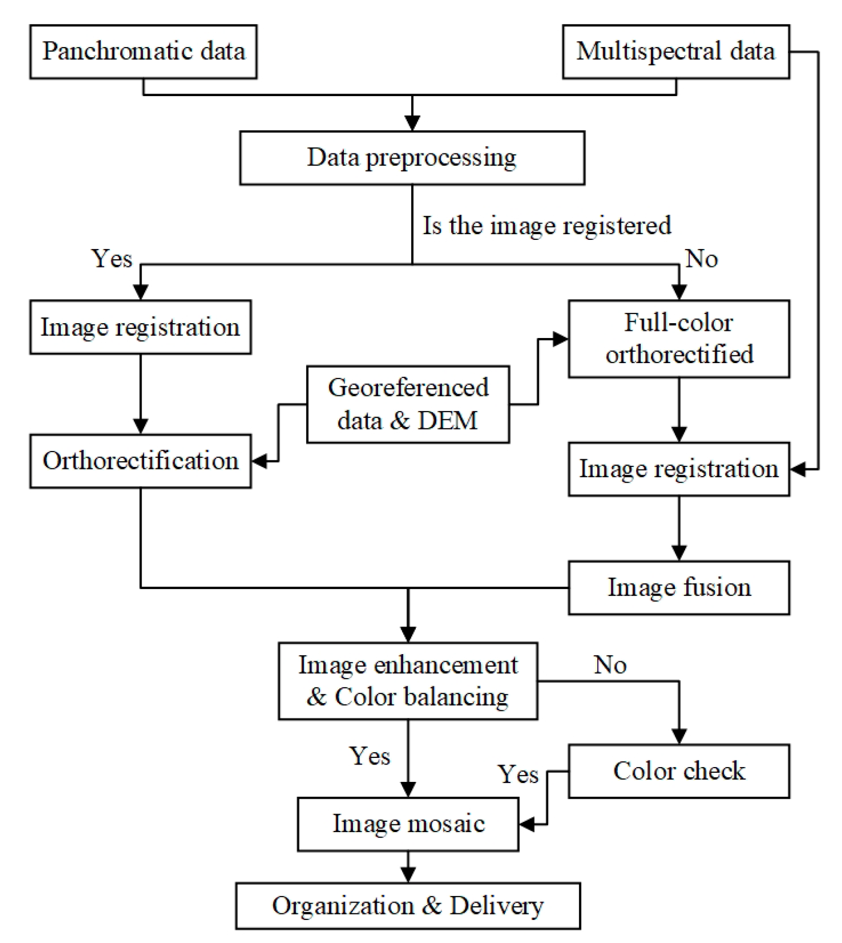
The raw remote sensing data underwent pre-processing steps including orthorectification, image registration, image fusion, enhancement, and mosaicking, resulting in base maps suitable for human–computer interactive interpretation (see Figure 3). Orthorectification: conducted using the “RPC + DEM + GCP” method in ERDAS IMAGINE 9.2 software to improve final geolocation accuracy. RPC: rational polynomial coefficients (rational function model). DEM: high-precision digital elevation model generated from IRS-P5. GCP: ground control points derived from recent topographic maps.

The orthorectification process in ERDAS IMAGINE is primarily based on transforming a central projection image into an orthographic projection through digital correction techniques. This procedure is designed to eliminate geometric distortions resulting from terrain variations, sensor misalignments, and other external influences, thereby ensuring that the corrected image adheres to orthographic projection standards.

The underlying principle involves subdividing the image into small segments and applying mathematical models to resolve the projection relationships. Using imaging parameters, ground control points (GCPs), and DEM, the system calculates corrections via conformal equations or other geometric transformation methods. These corrections are then applied to reconstruct a geometrically accurate, terrain-adjusted image.

The formula typically used for ERDAS ortho-correction is as follows:

(1)

Geometric correction formula: in geometric correction, the transformation relationship between image coordinates and map coordinates can be expressed as a polynomial:

$$x=f_x(u,v)={\displaystyle \sum _{i=0}^n}{\displaystyle \sum _{j=0}^{n-i}}{a}_{ij}{u}^i{v}^j$$

(1)

$$y=f_y(u,v)={\displaystyle \sum _{i=0}^n}{\displaystyle \sum _{j=0}^{n-i}}{b}_{ij}{u}^i{v}^j$$

(2)

where x and y are map coordinates, u and v are image coordinates, and a_ij and b_ij are coefficients.

(2)

Root Mean Square Error (RMSe) formula: used to evaluate the accuracy of the calibration

$$RMSe=\sqrt{{(x_r-x_i)}^2+{(y_r-y_i)}^2}$$

(3)

where x_i and y_i are the coordinates of the input image and x_r and y_r are the coordinates of the reference image. In practice, ERDAS provides a variety of tools and modules to support ortho-correction.

The image fusion process involves several key stages: pre-fusion image processing, selection of optimal fusion algorithms, implementation, and post-fusion quality verification. Pre-fusion procedures enhance local grayscale contrast to accentuate texture details and boost texture energy, while minimizing noise through targeted refinements. Color enhancement plays a critical role during this phase, adjusting brightness, hue, and saturation to improve color differentiation among terrain features. Common fusion methods include the following: IHS transformation; principal component transformation; weighted multiplication; ratio transformation; wavelet transformation; high-pass filtering; Brovey transform; Gram–Schmidt spectral sharpening; and PANSHARP fusion combining RGB and IHS transformations.

Fusion method selection is adapted to varying weather conditions. Post-fusion images often require tonal correction due to challenges such as low brightness, limited dynamic range, and insufficient color richness. Enhancement techniques applied at this stage include linear and non-linear stretching, brightness–contrast adjustment, color balancing, and modification of hue–saturation–lightness parameters.

Mosaicking begins with individual datasets undergoing tonal adjustment to ensure internal consistency within each scene or strip. Overlapping regions between scenes are then used to guide global tonal harmonization through joint adjustment strategies. When automatic approaches—such as histogram equalization or matching—fail due to temporal inconsistencies, manual color correction is performed using Photoshop software.

Ensuring data accuracy throughout the monitoring process is essential to maintaining the reliability of analytical outcomes. However, due to technical limitations and algorithmic design constraints, monitoring equipment may introduce truncation errors, which compromise data precision. These errors typically originate from three primary sources: numerical accuracy limitations, errors in the data format conversion process, and quantization errors. For this reason, the impact of truncation error on the decoding results is minimized by choosing four methods: appropriate resolution, multi-temporal data comparison, image pre-processing, and multi-source data fusion in this paper. The list of symbols of some formulas are shown in

Table 3. List of symbols.

Nomenclature
Etruncation	truncation error
Econversion	conversion error
Equantization	quantization error
f	floating-point number
|f|	the rounded portion of the floating-point number
a	acquired data
c	system accuracy
Q	quantization step size

.

The truncation error expression is given below,

$$E_{truncation}=a-round(a/c)\times c$$

(4)

where E_truncation is the truncation error, a is the acquired data, and c is the system accuracy.

Data format conversion error usually occurs in the process of converting floating point numbers to integers; the fractional part is discarded, thus affecting the integrity of the data. The theoretical formula is expressed as follows:

$$E_{conversion}=f-\left|f\right|$$

(5)

where E_conversion is the conversion error, f is a floating-point number, and |f| is the rounded portion of the floating-point number.

Quantization error, on the other hand, occurs during the digitization of analog signals, where larger quantization steps may result in the loss of certain details of the signal, affecting the fineness of the data with the following equation:

$$E_{quantization}=a-round(a/Q)\times Q$$

(6)

where E_quantization is the quantization error and Q is the quantization step size.

4. Remote Sensing Survey and Analysis of Thermokarst Hazards in Qinghai

4.1. Remote Sensing Image Characteristics of Thermokarst Hazards

The analysis of topographic and geomorphic characteristics in remote sensing imagery is essential for elucidating their role in the various stages of landslide evolution. Additionally, the characterization of surface deformation plays a pivotal role in understanding the dynamic processes of landslide development.

Specifically, the visual content of elevation-based images—where color gradation corresponds to elevation values—changes markedly before and after deformation events. These changes are primarily reflected in the variation of pixel grayscale values at identical spatial locations, indicating surface displacement or structural alteration. The process of comparative analysis is as follows:

(1)

Match the two images with accurate guaranteed spatial alignment in order to facilitate the comparison of pixel points at the same location.

(2)

Calculate the difference in gray value of each pixel point at each corresponding location with the following formula:

$$\Delta L\left(P\right)=|L{T}_2\left(P\right)-L{T}_1\left(P\right)|$$

(7)

where LT₁(P) and LT₂(P) are distributed as the gray value at the pixel point P at the moment of T₁ and T₂; ∆L(P) is the difference of the gray value at the pixel point.

Thermokarst hazards exhibit distinct features in remote sensing imagery, with their intrinsic physical characteristics strongly reflected in visual data. Through systematic interpretation, this study identified a range of permafrost-related hazard types, including the following: retrogressive thaw slumps (including fine-grained soil slumps, coarse-grained soil slumps, and thaw-induced landslides), gelifluction flows (comprising flow tongues, alluvial fans, terraces, and fish-scale turf patterns), bedrock landslides, debris flows, and frost mounds. Identification relies on analyzing geometric, spectral, and textural attributes (shape, size, tone, texture, roughness, and contrast) displayed on high-resolution imagery.

RTS—also referred to as headward thaw flow landslides—develop when subsurface ice becomes exposed due to natural or anthropogenic disturbances. During thaw seasons, the melting of ground ice leads to the collapse of overlying active layers. The displaced material, typically in a viscous-plastic state, creeps downslope, temporarily covering exposed ice while progressively revealing new ice surfaces. This process propagates upslope, from the toe toward the crest. Based on field observations, RTS are classified into the following three types. Fine-grained soil slumps: these occur on gentle slopes with slow movement rates and limited displacement and are characterized by finer soil textures. Coarse-grained soil slumps: composed of frost-weathered coarse debris, developing under similar slope conditions as fine-grained types. Thaw-induced landslides: these are found on steeper slopes, exhibiting sudden failures with longer runout distances. Remote sensing identification markers reflect RTS morphological signatures through the following: geometric features—slope deformation patterns; spectral responses—tone anomalies between slumped and intact areas; and ecological disruptions—vegetation loss and drainage alterations.

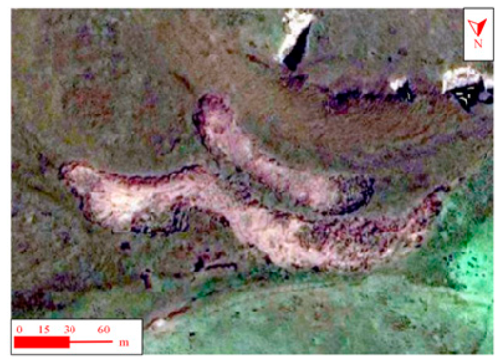
4.1.1. Tone Signatures

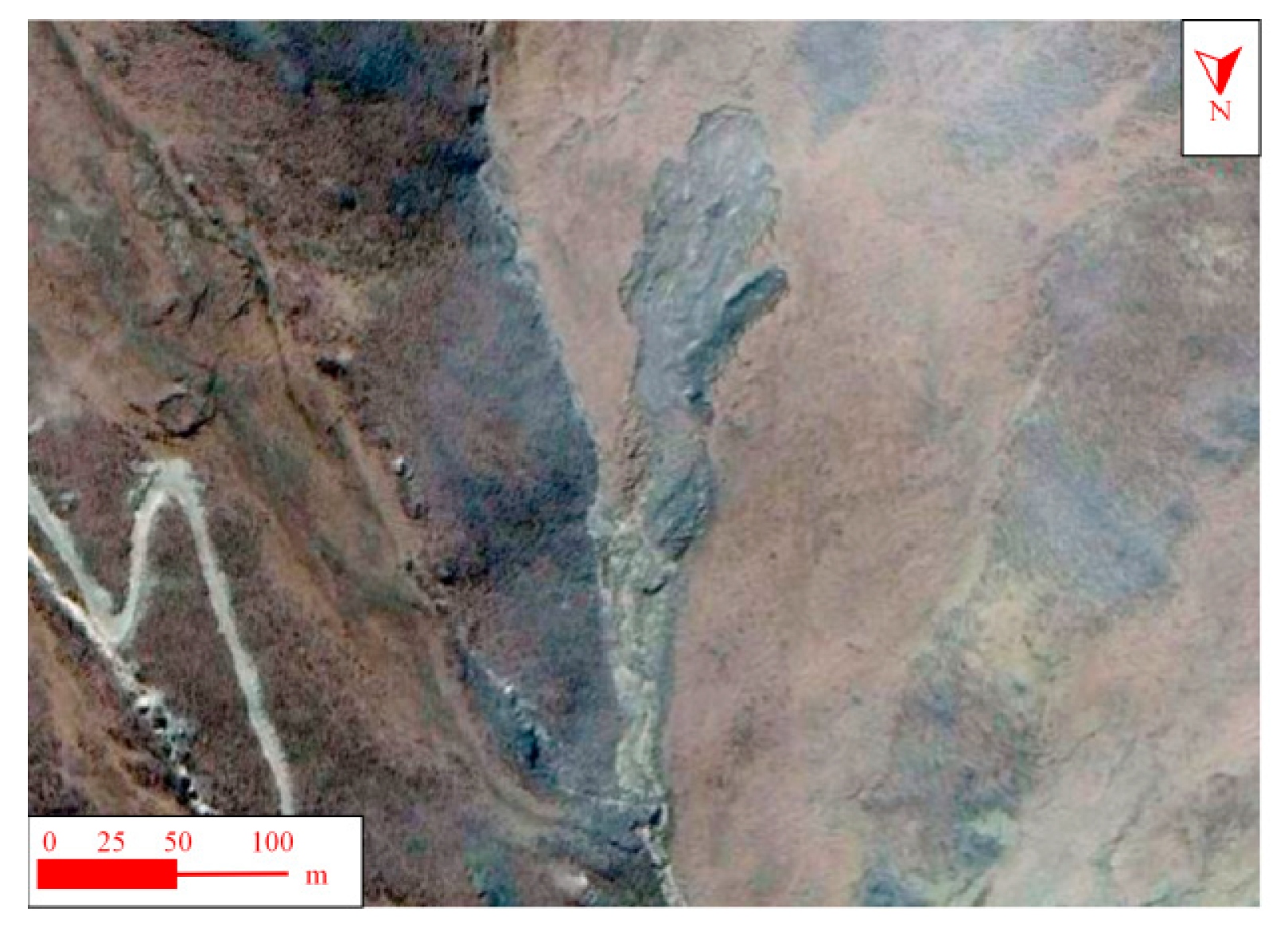
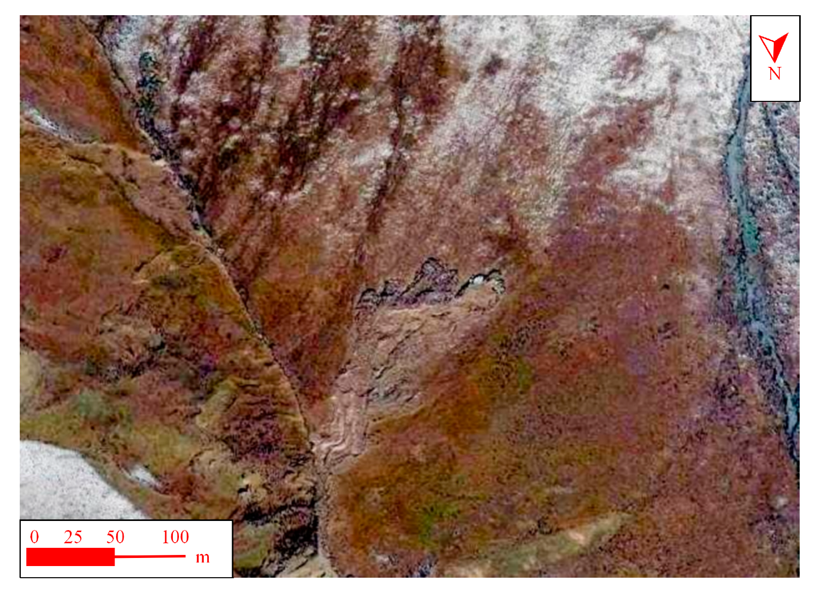
Tonal variation serves as a key diagnostic feature in remote sensing-based identification of thermokarst-related slump activity. Slump movements produce distinct tonal contrasts relative to surrounding terrain, aiding in both classification and temporal staging. Exposed soils typically display dark gray (fine-grained slumps, Figure 4), or gray-white, or reddish-brown hues (coarse-grained slumps/landslides, Figure 5). Incipient slumps exhibit crescent-shaped tonal anomalies at headwalls/toes with vegetated midslopes. Active slumps show full-length exposure with pronounced tonal deviations.

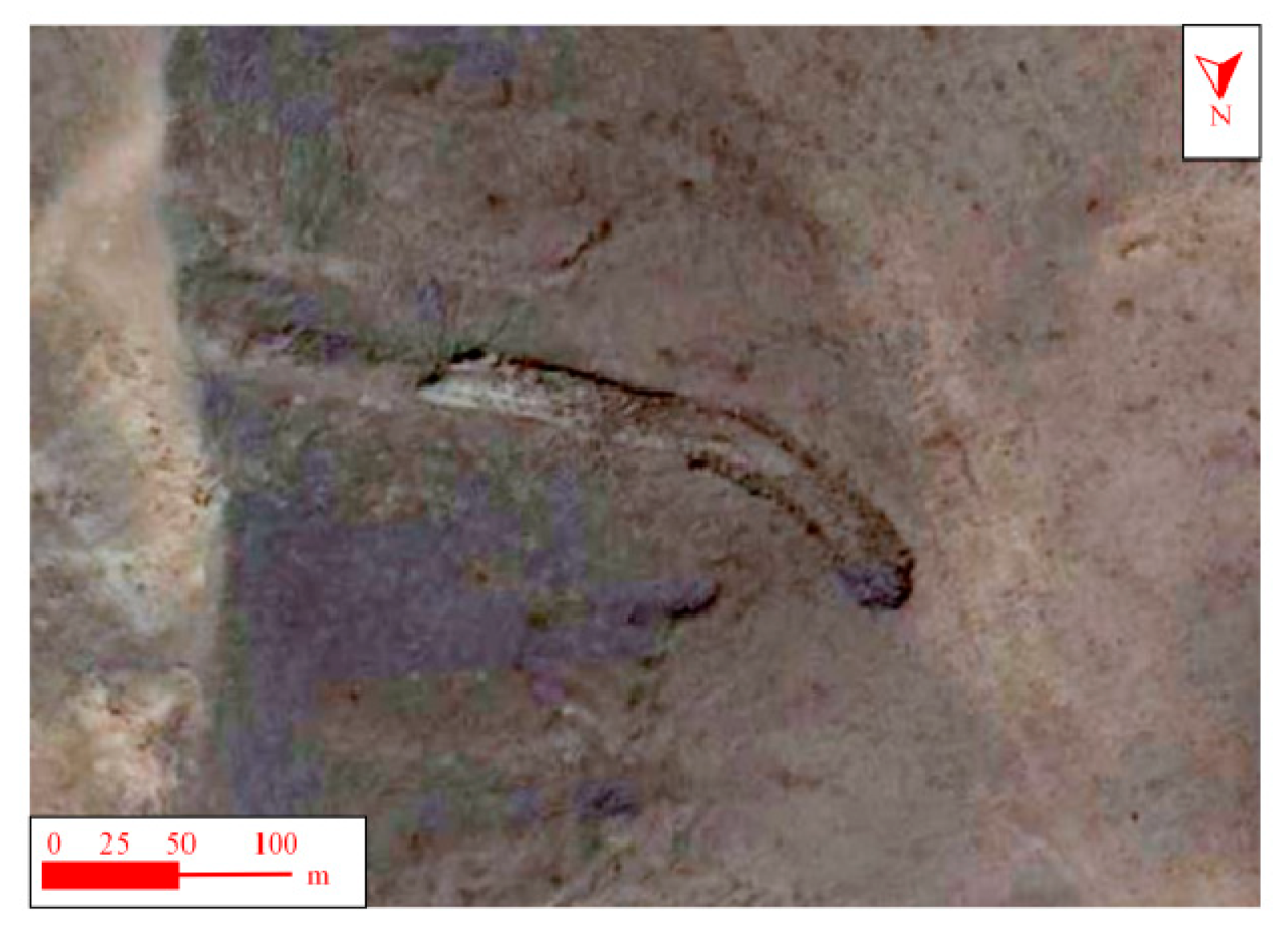
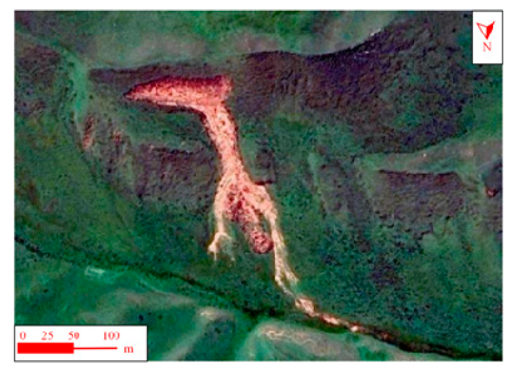
4.1.2. Morphological Signatures

Slump masses commonly exhibit a variety of planar configurations, including linear, elliptical, inverted pear-shaped, tongue-like, stepped, branched, elongated, multi-tongued, and serrated morphologies. Early-stage slumps tend to display regular geometries—such as elliptical, inverted pear-shaped, and tongue-like formations—with relatively limited spatial dimensions (see Figure 6). Mid- to late-stage slumps evolve through progressive headward erosion and downslope creep, resulting in irregular morphologies, including linear, stepped, branched, elongated, multi-tongued, and serrated patterns, often with significantly expanded spatial scales (see Figure 7). Thaw-induced landslides, typically occurring on steeper slopes, frequently adopt linear, branched, or elongated configurations due to their greater runout distances (see Figure 8).

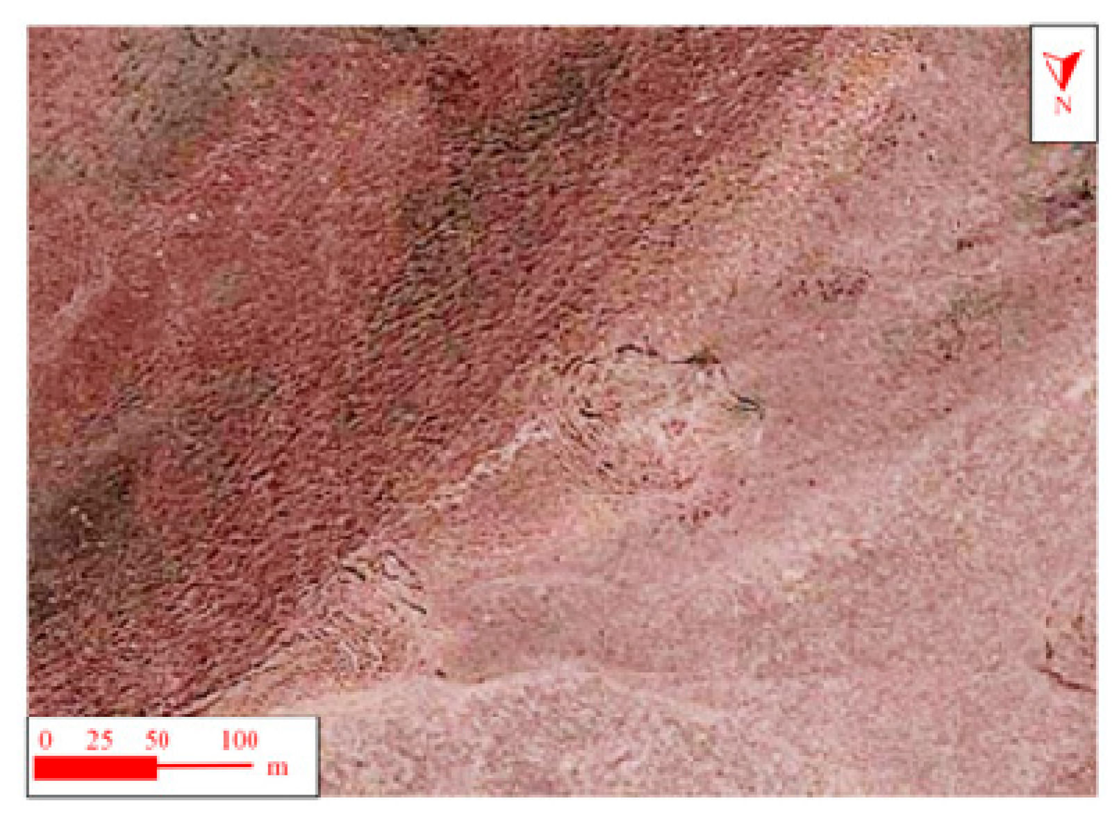
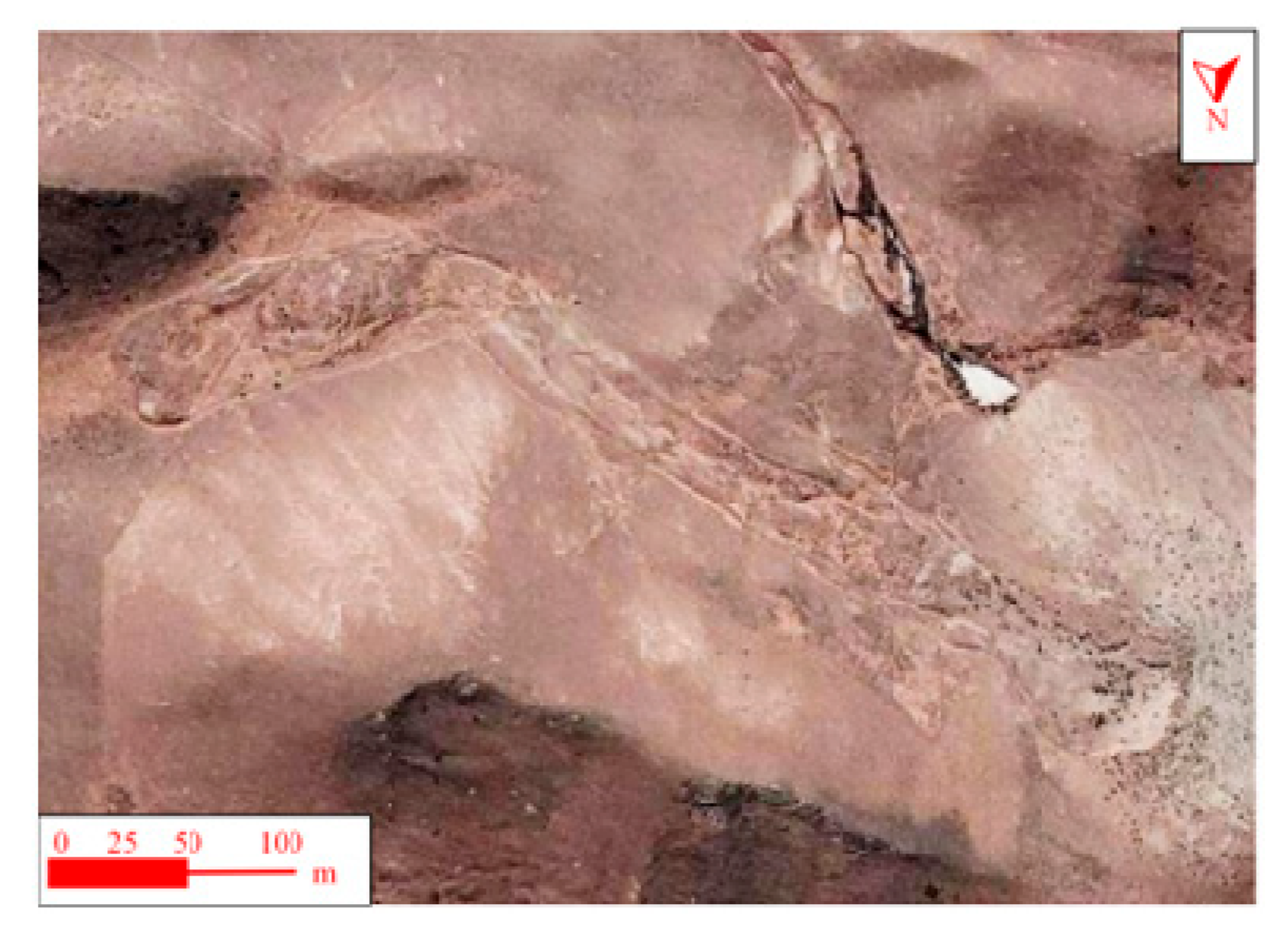
4.1.3. Textural Signatures

Slump activity markedly alters the original surface texture, producing rough and disordered patterns with sharply defined boundaries. The presence of arcuate transverse ridges and flow traces across slump surfaces signals active downslope creep behavior. Additionally, compressional accumulation near the frontal margins results in the formation of arc-shaped transverse textures, indicative of internal stress redistribution and slope deformation. Fine-grained and coarse-grained slumps exhibit short displacement distances, concentrated debris accumulation, and prominent transverse arcuate textures (Figure 9). Thaw-induced landslides demonstrate dispersed debris distribution, underdeveloped transverse textures, and linear longitudinal ridges along flanks (Figure 10).

4.1.4. Geomorphological Signatures

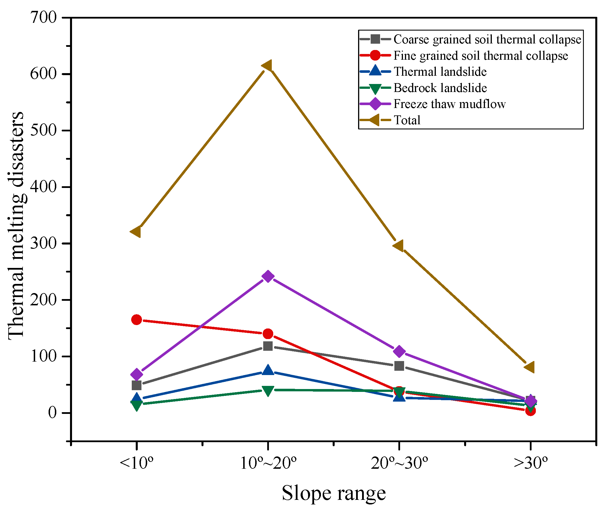
Retrogressive thaw slumps predominantly develop on gentle slopes (<16°) with thick fine-grained deposits and ice-rich substrates. Thaw-induced landslides may occur on steeper slopes (>16°) (Figure 11), while fine-grained and coarse-grained slumps are generally confined to slopes <16° (Figure 12).

Slump activities disrupt original geomorphic units, causing abrupt slope profile alterations. A distinct scarp (arcuate, armchair-shaped, or serrated) typically marks the headwall region (Figure 13), with crescent-shaped or serrated fissures characterizing initial development stages. Slump surfaces often exhibit gently terraced topography with local transverse ridges. Frontal zones display tongue-shaped or fan-shaped accumulation areas bounded by steep slopes or scarps. Figure 14 and Figure 15 show the thermal collapse of developed and undeveloped vegetation, respectively.

4.2. Distribution Characteristics of Thermokarst Hazards in Qinghai

Utilizing Landsat-8 data across Qinghai Province, supplemented by Google Earth, GF-2, GF-1, and ZY-3 imagery in selected areas, remote sensing interpretation of thermokarst hazards was conducted in permafrost regions. The interpretation covered hazard types including retrogressive thaw slumps, gelifluction flows, thaw-induced landslides, bedrock landslides, and debris flows. The total interpreted area spanned 35.7 × 10⁴ km², with 1321 hazard sites identified.

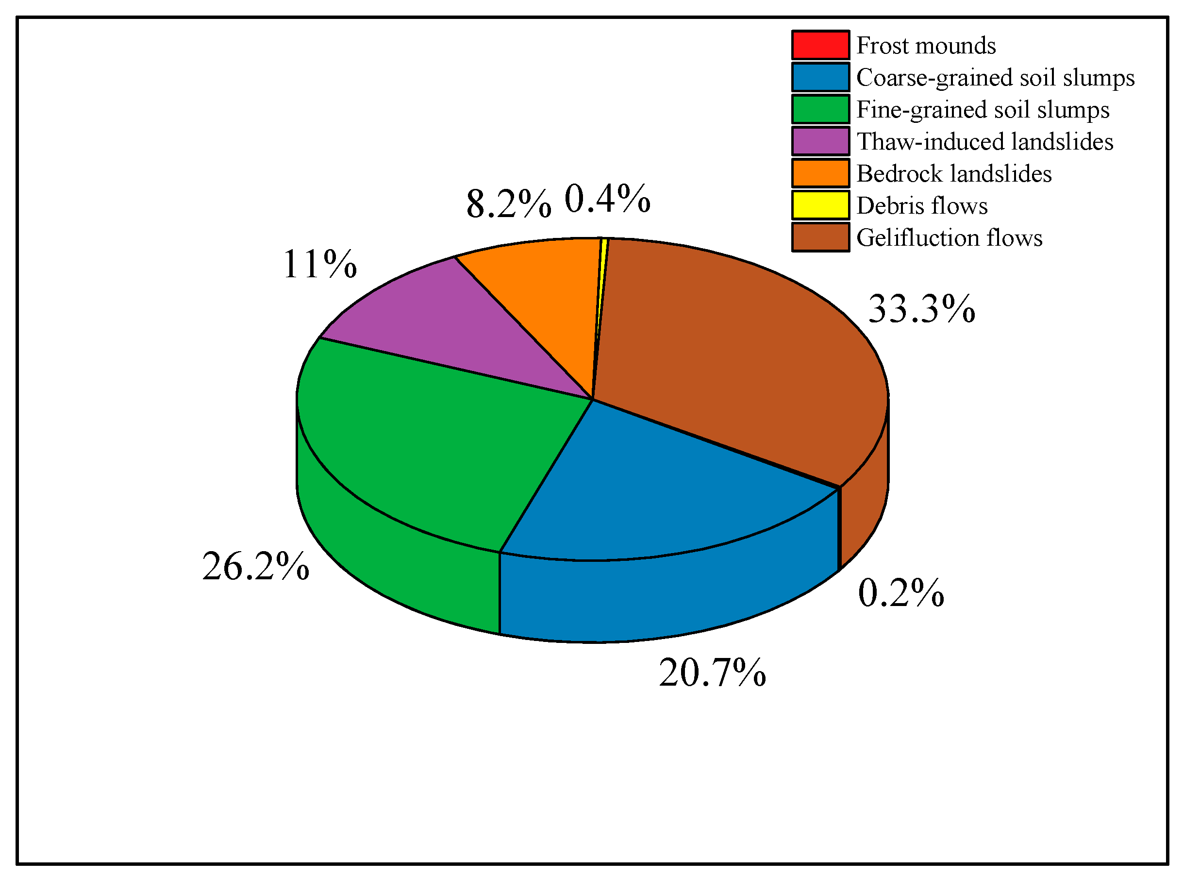
This remote sensing interpretation identified 1321 thermokarst hazard sites, comprising 273 coarse-grained soil slumps (20.7% of total), 346 fine-grained soil slumps (26.2%), 146 thaw-induced landslides (11%), 108 bedrock landslides (8.2%), 5 debris flows (0.4%), 440 gelifluction flows (33.3%), and 3 frost mounds (0.2%) (Figure 16). Debris flows showed limited permafrost correlation and were not prioritized in this investigation. Frost mound interpretation was restricted due to their small scale (<10 m diameter), indistinct image features, and data resolution constraints.

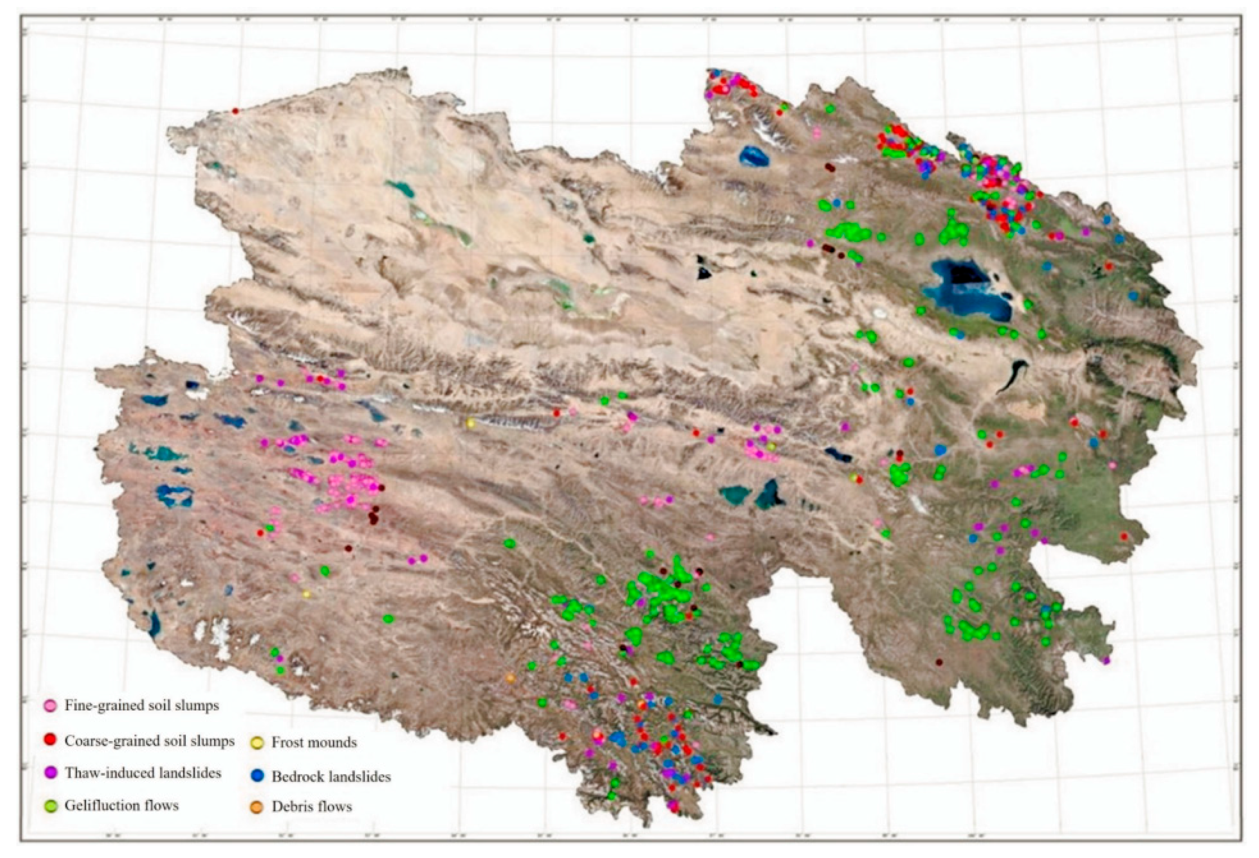
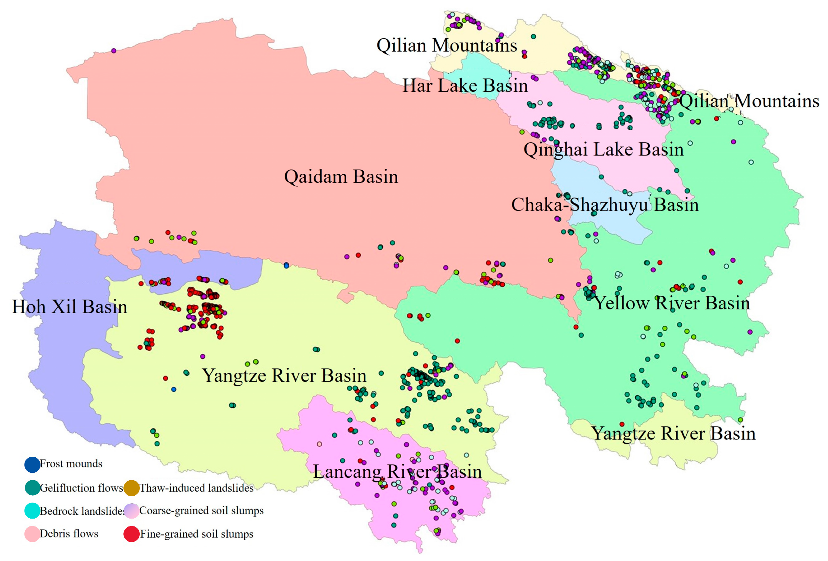
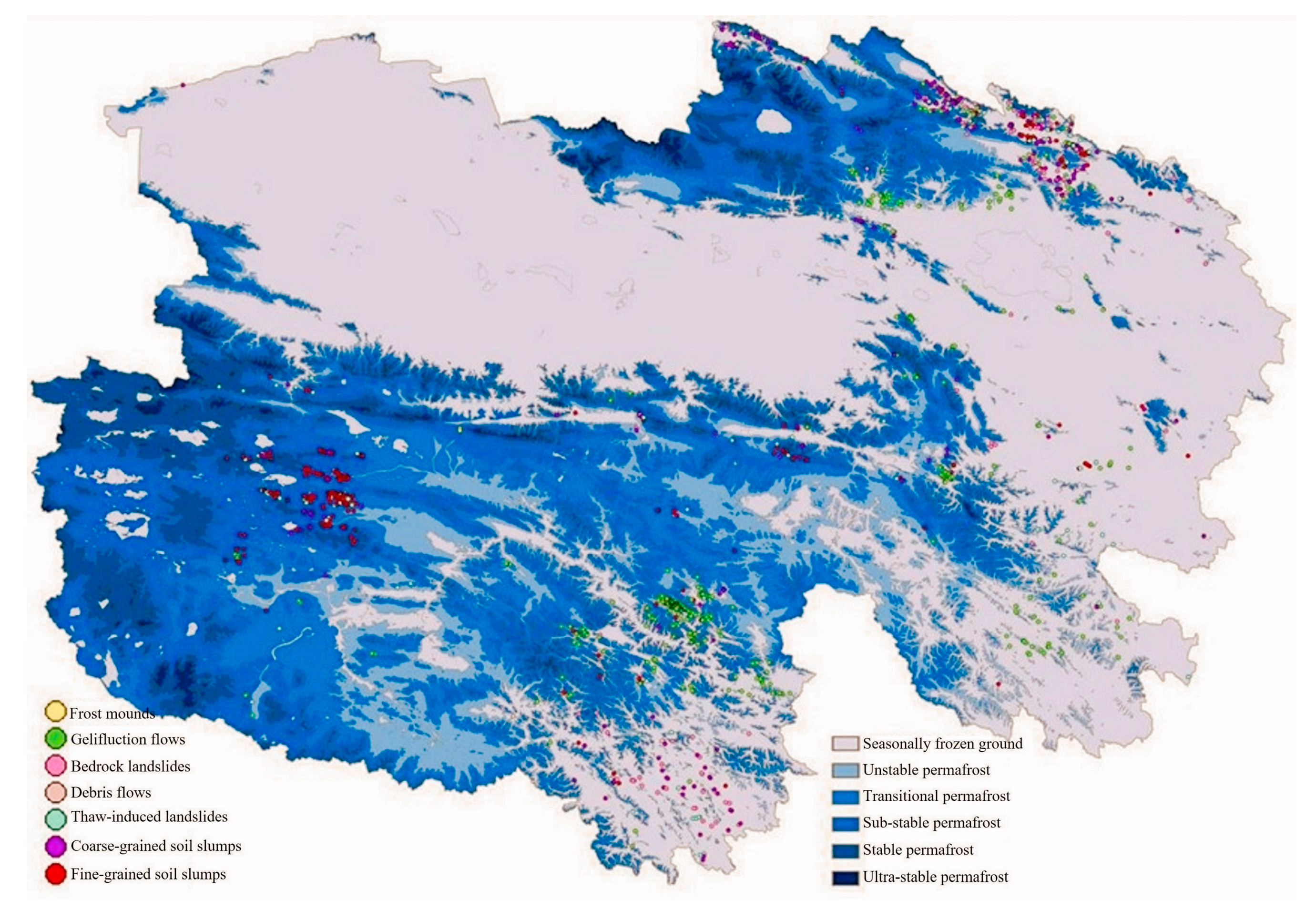
Thermokarst hazards are widely distributed across all permafrost regions of Qinghai Province, with notable concentrations in the Qilian Mountains, Hoh Xil region, and the Tongtian River Basin. In contrast, other areas exhibit more sporadic occurrences.

Retrogressive thaw slumps are primarily concentrated in the Qilian Mountains and Hoh Xil region, reflecting the geomorphic and climatic conditions conducive to ice-rich permafrost degradation. Meanwhile, gelifluction flows are predominantly observed within the Tongtian River Basin, where slope morphology and seasonal thawing promote their formation (see Figure 17).

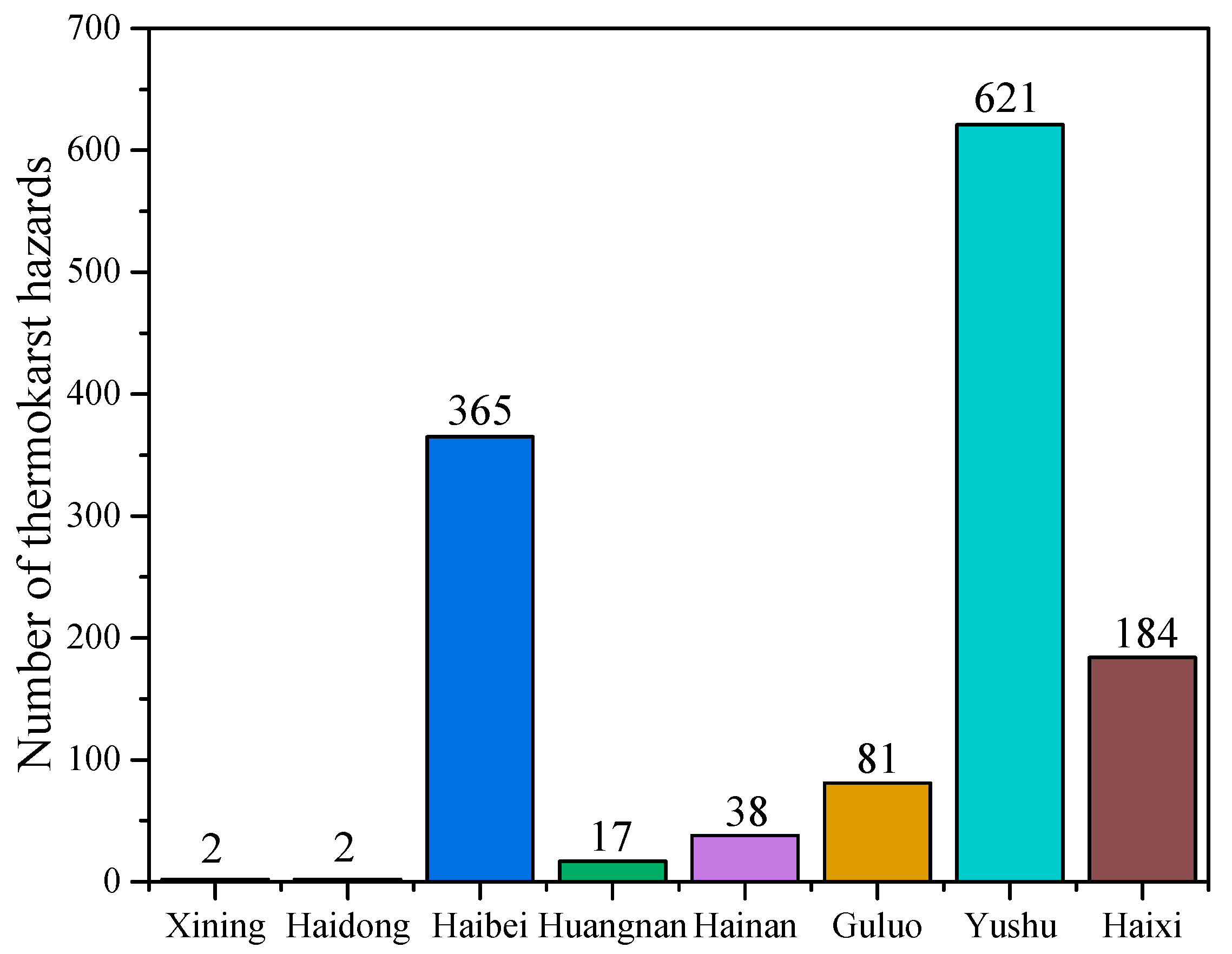
Thermokarst hazards are distributed across eight prefectures in Qinghai Province as follows: Yushu Tibetan Autonomous Prefecture: 621 sites (47.3% of provincial total), predominantly fine-grained soil slumps and gelifluction flows. Haibei Tibetan Autonomous Prefecture: 365 sites (27.8%), mainly coarse-grained soil slumps. Haixi Mongol and Tibetan Autonomous Prefecture: 187 sites (14.24%). Golog Tibetan Autonomous Prefecture: 81 sites (6.17%). Hainan Tibetan Autonomous Prefecture: 38 sites (2.89%). Huangnan Tibetan Autonomous Prefecture: 17 sites (1.29%). Xining City: 2 sites (0.15%). Haidong City: 2 sites (0.15%) (Figure 18).

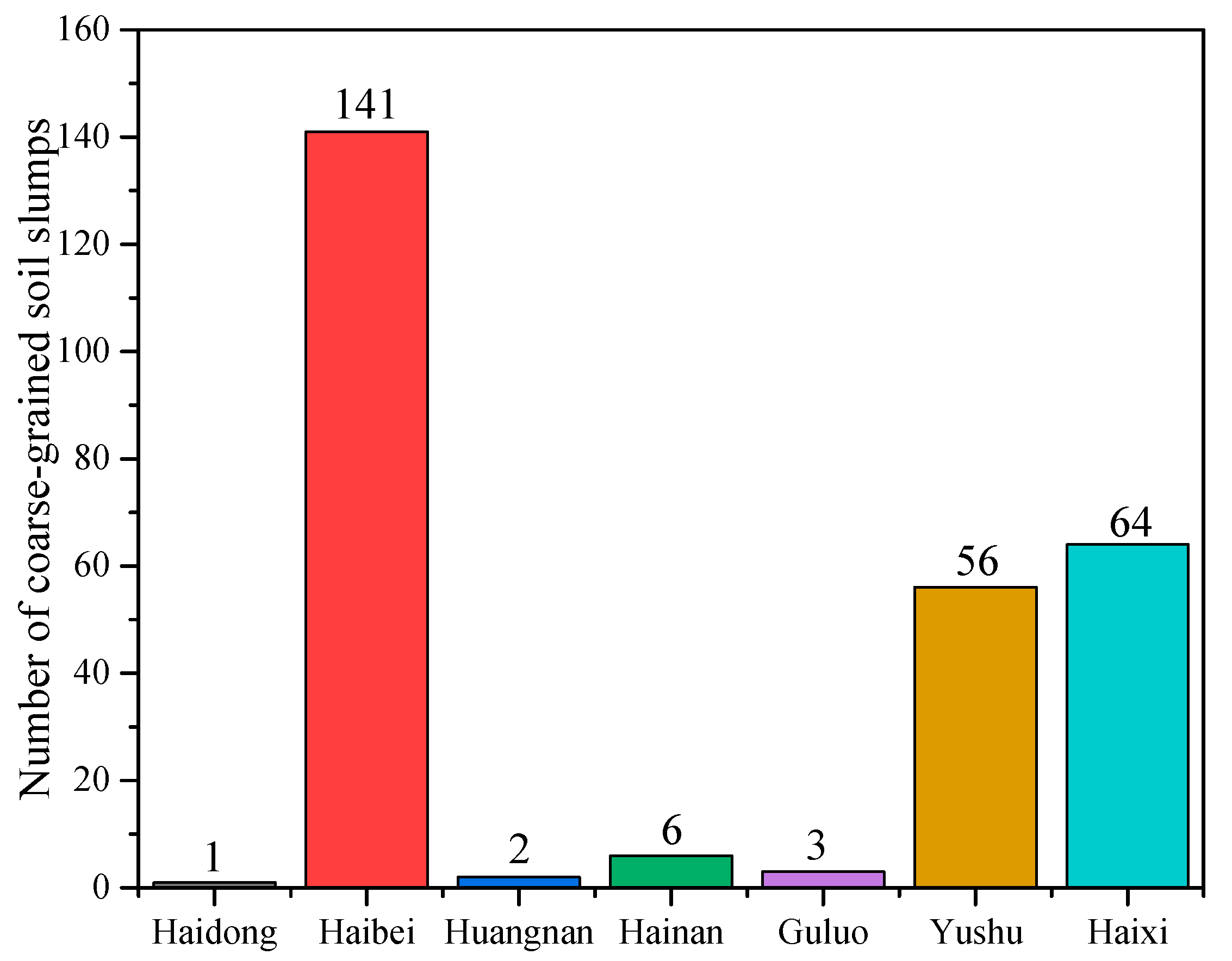
Coarse-grained soil slumps (273 sites): predominantly distributed in Haibei (141 sites, 51.65%), Haixi (64 sites, 23.44%), and Yushu (56 sites, 20.51%). Minor occurrences: Hainan (6, 2.2%), Goluo (3, 1.1%), Huangnan (2, 0.73%), and Haidong (1, 0.37%). No occurrences in Xining (Figure 19).

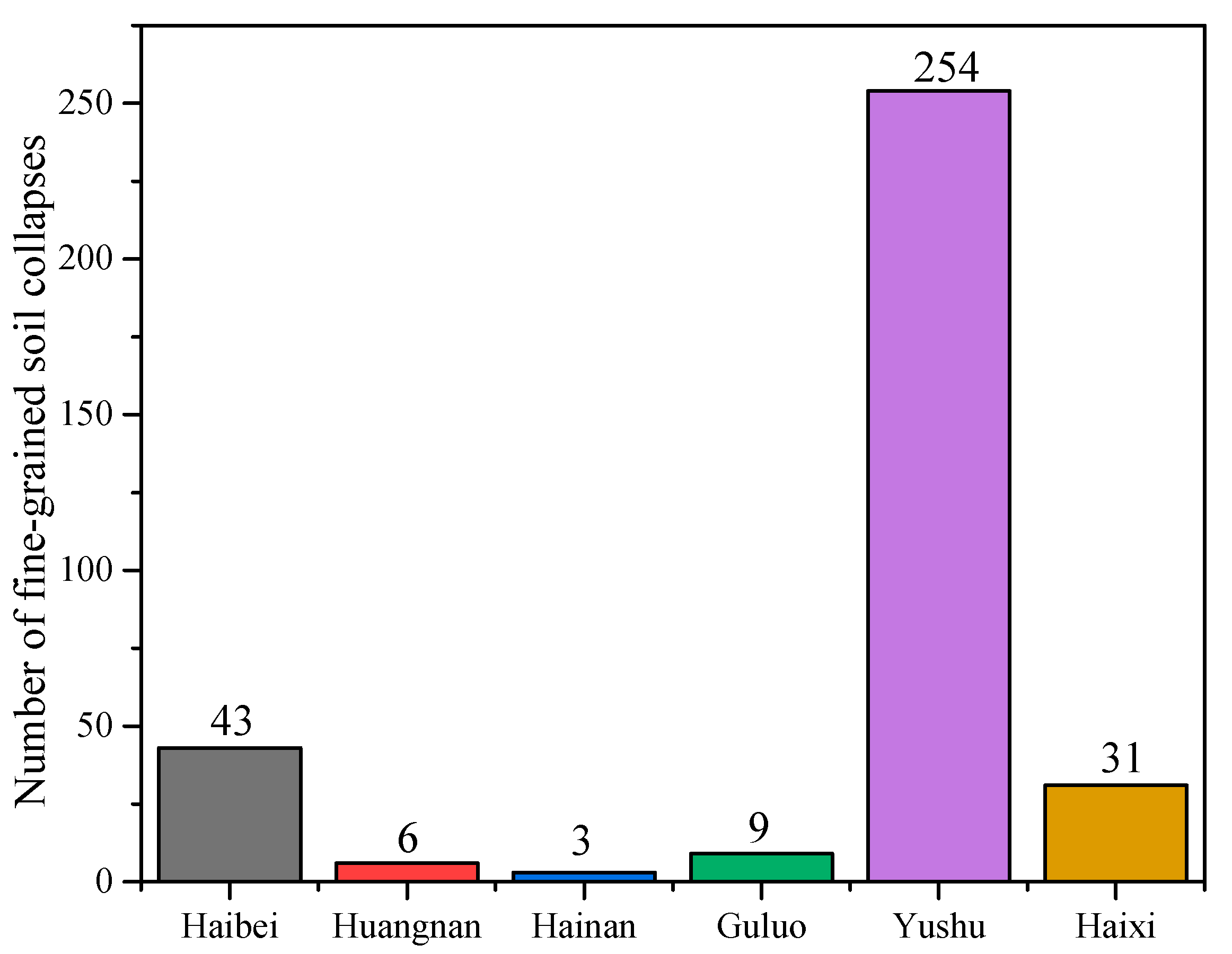
Fine-grained soil slumps (346 sites): concentrated in Yushu (254, 73.41%), with secondary clusters in Haibei (43, 12.43%) and Haixi (31, 9%). Minor distributions: Golog (9, 2.6%), Huangnan (6, 1.73%), and Hainan (3, 1.73%). Absent in Xining/Haidong (Figure 20).

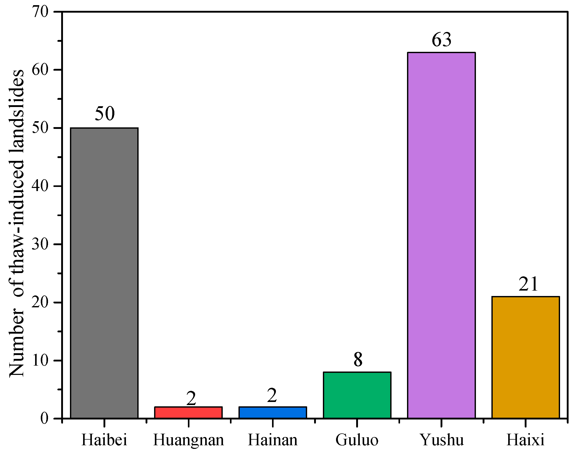
Thaw-induced landslides (146 sites): primary distribution in Yushu (63, 43.15%) and Haibei (50, 34.25%). Secondary clusters: Haixi (21, 14.38%), Golog (8, 5.48%), Huangnan (2, 1.37%), and Hainan (2, 1.37%). Absent in Xining/Haidong (Figure 21).

Thermokarst hazards are primarily concentrated in three prefectures of Qinghai Province: Yushu Tibetan Autonomous Prefecture, Haibei Tibetan Autonomous Prefecture, and Haixi Mongol and Tibetan Autonomous Prefecture. In contrast, Xining and Haidong cities display minimal occurrences. 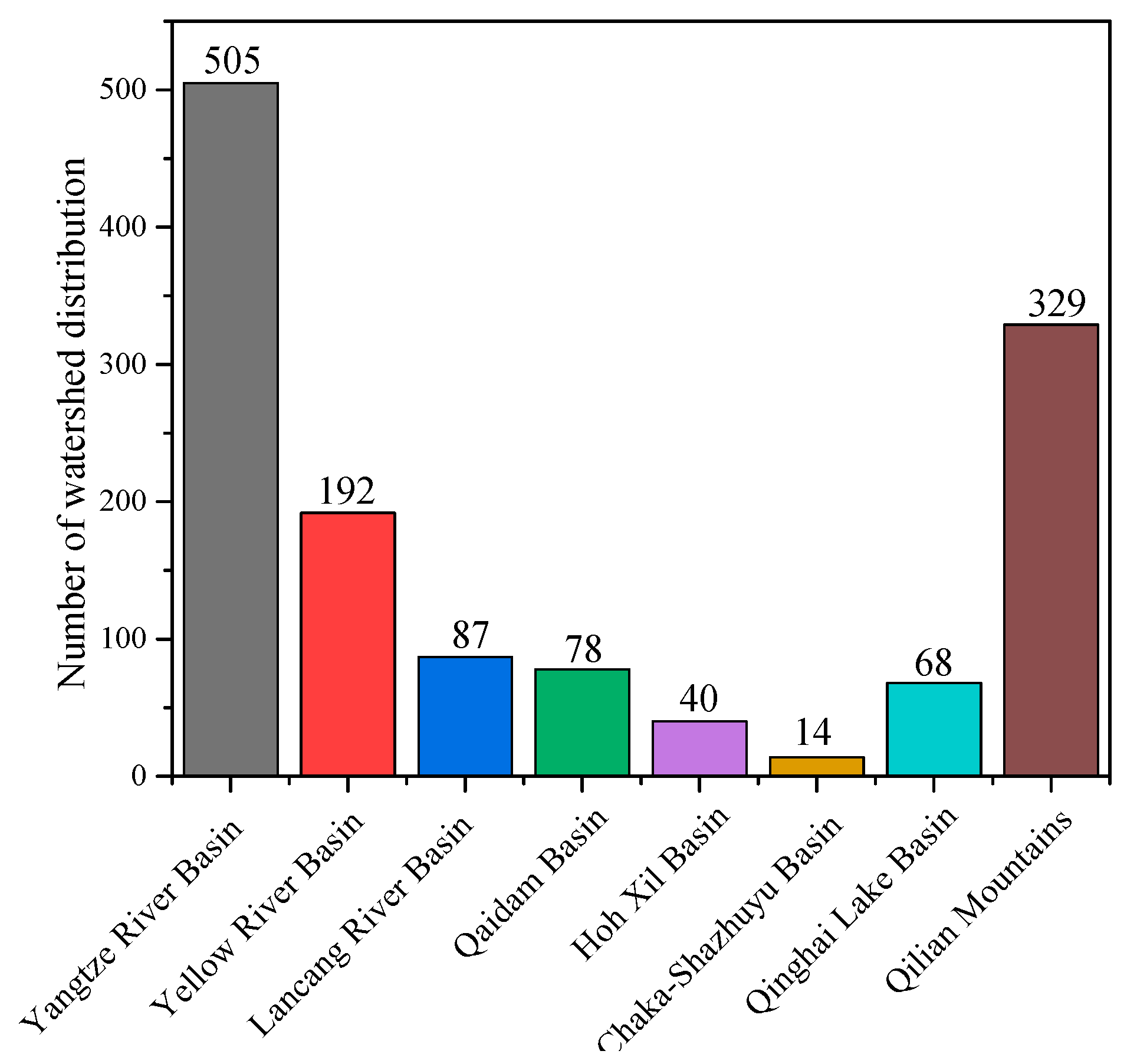Type-specific distributions are as follows: coarse-grained soil slumps: Haibei/Haixi/Yushu; fine-grained soil slumps: Yushu; thaw-induced landslides: Yushu/Haibei; bedrock landslides: Haibei/Yushu; gelifluction flows: Yushu, Figure 22. Watershed distribution (Figure 23): Yangtze River Basin: 505 sites (38.46%); Qilian Mountains: 329 sites (25.06%); Yellow River Basin: 192 sites (14.62%); Lancang River Basin: 87 sites (6.63%); Qaidam Basin: 78 sites (5.94%); Qinghai Lake Basin: 68 sites (5.12%); Hoh Xil Basin: 40 sites (3.05%); Chaka-Shazhuyu Basin: 14 sites (1.07%); and Har Lake Basin: no hazard sites (Figure 23).

Spatial Distribution Patterns. Coarse-grained soil slumps: predominantly in exorheic basins (Yangtze, Yellow, and Lancang River Basins); fine-grained soil slumps: mainly Yangtze River Basin; thaw-induced landslides: primarily Yangtze River Basin; bedrock landslides: concentrated in Qilian Mountains, Yellow River Basin, and Lancang River Basin; gelifluction flows: dominant in Yangtze River Basin.

The 1321 interpreted thermokarst hazards exhibit clustered distribution across Qinghai’s permafrost regions. High-density clusters occur in Zhiduo County, Qilian County, and Qumalai County. Coarse-grained slumps: Qilian County and Tianjun County; fine-grained slumps: Zhiduo County and Qilian County; thaw landslides: Qilian County and Zhiduo County; bedrock landslides: Qilian County and Nangqian County; gelifluction flows: Qumalai County and Qilian County. Watershed-wise, hazards concentrate in the Yangtze River Basin (38.46%) and Qilian Mountains (25.06%).

5. Case Analysis of Thermal Melt Disaster

5.1. Distribution Characteristics of Thermal Melting Disasters in Different Types of Frozen Soil Areas

In order to explore the correlation between permafrost stability and thermal karst disasters, we used a machine learning model to conduct an in-depth analysis of multi-source data. By integrating the data of remote sensing images, surface temperature, soil moisture and disaster history records in permafrost regions, a prediction model was constructed by using random forest, gradient boosting, and other algorithms to quantify the correlation between different stability grades of frozen soil (such as extremely stable, stable, sub-stable, transitional, and unstable) and thermal karst disasters (such as thermal thaw collapse of coarse-grained soil, thermal thaw collapse of fine-grained soil, thermal thaw landslide, bedrock landslide, and freeze–thaw mud flow). It provides data support and a scientific basis for ecological protection and disaster risk early warning in permafrost regions.

As shown in Figure 24 and Figure 25 and

Table 4. Classification and statistics of thermal thawing disasters in different types of frozen soil regions in Qinghai Province.

Types of Disasters		Coarse- Grained Soil Thermal Collapse	Fine- Grained Soil Thermal Collapse	Thermal Landslide	Bedrock Landslide	Freeze Thaw Mudflow	Total	Percentage of All Disasters (%)
Seasonal frozen soil area		168	62	70	76	226	602	45.85
Permafrost region	Unstable frozen soil area	44	20	20	21	151	256	19.5
	Transitional permafrost zone	30	81	20	10	44	185	14.09
	Metastable frozen soil area	25	178	29	1	18	251	19.11
	Stable frozen soil area	5	6	7	0	1	19	1.45
	Extremely stable frozen soil area	0	0	0	0	0	0	0
	Subtotal	104	285	76	32	214	711	54.15
Total		272	347	146	108	440	1313	100

Note: The table does not include statistics on mudslides and frost heave mounds, with 5 mudslides and 3 frost heave mounds, resulting in a total of 1321 interpreted disasters.

, thermokarst hazards predominantly occur in seasonally frozen ground, unstable permafrost zones, transitional permafrost zones, and sub-stable permafrost zones. The distribution is as follows: seasonally frozen ground: 602 sites (45.85% of total); unstable permafrost: 256 sites (19.5%); transitional permafrost: 185 sites (14.09%); sub-stable permafrost: 251 sites (19.11%); stable permafrost: 19 sites (1.45%); and ultra-stable permafrost: no hazards observed.

Figure 25 demonstrates regional patterns. Qilian Mountains, Yushu, and Golog regions: hazards concentrated in seasonally frozen ground; Hoh Xil region: hazards mainly distributed in transitional and sub-stable permafrost zones.

Coarse-grained soil slumps (272 sites). Seasonally frozen ground: 168 sites (61.76%); permafrost zones: 104 sites (38.24%); unstable permafrost: 44 (16.18%); transitional permafrost: 30 (11.03%); sub-stable permafrost: 25 (9.19%); stable permafrost: 5 (1.84%); and ultra-stable permafrost: none.

Fine-grained soil slumps (347 sites). Seasonally frozen ground: 62 (17.87%); permafrost zones: 285 (82.13%); unstable permafrost: 20 (5.76%); transitional permafrost: 81 (23.34%); sub-stable permafrost: 178 (51.3%); stable permafrost: 6 (1.73%). Ultra-stable permafrost: none.

Thaw-induced landslides (146 sites). Seasonally frozen ground: 70 (46.95%); permafrost zones: 76 (52.05%); unstable permafrost: 20 (13.7%); transitional permafrost: 20 (13.7%); sub-stable permafrost: 29 (19.86%); stable permafrost: 7 (4.79%); and ultra-stable permafrost: none.

Analysis of slope distribution across 1,313 interpreted thermokarst hazards (

Table 5. Classification and statistics of thermal and thermal disasters in different slope sections of Qinghai Province.

Slope Range (°)	Coarse-Grained Soil Thermal Collapse	Fine-Grained Soil Thermal Collapse	Thermal Landslide	Bedrock Landslide	Freeze Thaw Mudflow	Total	Percentage of All Disasters (%)
≤10	49	165	24	15	68	321	24.45
10-20	118	140	74	41	242	615	46.84
20-30	83	38	27	39	109	296	22.54
>30	22	4	21	13	21	81	6.17
Total	272	347	146	108	440	1313	100

Note: The table does not include statistics on mudslides and frost heave mounds, with 5 mudslides and 3 frost heave mounds, resulting in a total of 1321 interpreted disasters.

) reveals predominant occurrence on slopes ≤30°. 0–10° slope interval: 321 sites (24.45% of total hazards); 10–20° interval: 615 sites (46.84%); 20–30° interval: 296 sites (22.54%); >30° slopes: 81 sites (6.17%).

As demonstrated in Figure 26, while fine-grained soil slumps decrease in frequency with increasing slope gradients, other hazard types exhibit initial increases followed by reductions. Overall, 50% of surveyed hazards concentrate within the 10–20° slope range.

5.2. Relationship Between Thermal Melting Disasters and Slope Orientation

Statistical analysis of slope aspects for various thermokarst hazards (

Table 6. Classification and statistics of thermal and thermal disasters in different slope directions in Qinghai Province.

Slope Range (°)	Coarse-Grained Soil Thermal Collapse	Fine-Grained Soil Thermal Collapse	Thermal Landslide	Bedrock Landslide	Freeze Thaw Mudflow	Total	Percentage of All Disasters (%)
0-45°	58	54	22	14	83	231	17.59
45–90°	39	48	17	17	57	178	13.56
90–135°	17	33	18	13	22	103	7.84
135–180°	21	42	11	9	13	96	7.31
180–225°	21	29	11	10	15	86	6.55
225–270°	31	39	13	21	81	185	14.09
270–315°	47	44	25	13	104	233	17.75
315–360°	38	58	29	11	65	201	15.31
Total	272	347	146	108	440	1313	100

, Figure 27) demonstrates predominant development on north (N) and northwest (NW) facing slopes, with minimal occurrences on south (S) and southeast (SE) aspects.

Fine-grained soil slumps exhibit relatively uniform distribution across all slope aspects. Other hazard types follow the overall statistical pattern, predominantly developing on N and NW slopes while showing limited occurrence on south-facing slopes (Figure 28).

5.3. Relationship Between Thermal Melting Disasters and Altitude

Statistical analysis of elevation distribution for various thermokarst hazards (

Table 7. Classification and statistics of thermal and thermal disasters at different altitudes in Qinghai Province.

Altitude (m)	Coarse-Grained Soil Thermal Collapse	Fine-Grained Soil Thermal Collapse	Thermal Landslide	Bedrock Landslide	Freeze Thaw Mudflow	Total	Percentage of All Disasters (%)
3100–3300	8	2	2	7	4	23	1.75
3300–3500	44	13	17	9	14	97	7.39
3500–3700	71	28	28	22	38	187	14.24
3700–3900	35	17	17	28	48	145	11.04
3900–4100	28	3	15	14	38	98	7.46
4100–4300	19	2	5	10	41	77	5.87
4300–4500	23	19	6	9	147	204	15.54
4500–4700	23	74	20	7	83	207	15.77
4700–4900	11	170	22	2	16	221	16.83
4900–5100	10	19	14	0	11	54	4.11
Total	272	347	146	108	440	1313	100

, Figure 29) reveals concentrated occurrences within 3500–3900 m and 4300–4900 m elevation ranges, reflecting distinct spatial patterns. 3500–3900 m: predominant in the Qilian Mountains (northern Qinghai); 4300–4900 m: mainly in the Hoh Xil region (southern Qinghai).

Type-specific elevation distributions (Figure 30). Fine-grained soil slumps: 4500–4900 m; gelifluction flows: 4300–4700 m; coarse-grained soil slumps: 3500–3700 m; bedrock landslides: 3500–3900 m; thaw-induced landslides: indistinct distribution pattern. Fine-grained slumps and gelifluction flows: Southern Qinghai (Hoh Xil). According to the altitude distribution of disasters, coarse-grained slumps and bedrock landslides: northern Qinghai (Qilian Mountains).

Geographically, fine-grained soil slumps and gelifluction flows are concentrated in southern Qinghai, particularly the Hoh Xil region, which features high-altitude permafrost landscapes. In contrast, coarse-grained soil slumps and bedrock landslides are primarily observed in northern Qinghai, notably within the Qilian Mountains, aligning with lower elevation zones and differing geomorphic conditions.

6. Conclusions

This study began with a comprehensive review of existing research, followed by the acquisition of baseline imagery for the target area. Subsequently, an integrated approach was adopted, combining Geospatial Science (GS) and Geographic Information Systems (GIS) technologies. Remote sensing data were fused with multi-source datasets and processed through automated extraction techniques alongside human–computer interactive interpretation. Analytical efforts combined indoor assessments with field investigations.

Remote sensing interpretation and information extraction tasks were conducted using specialized platforms including ENVI, ERDAS, MAPGIS, and ArcGIS. To enhance spatial accuracy, a dual-zone strategy—targeting key areas and broader general zones—was implemented. Multi-temporal satellite imagery from key hazard zones facilitated the analysis of developmental trends over time.

Based on these methods, a comprehensive assessment of thermokarst hazards was completed. The key conclusions are as follows:

• Integrated application of Landsat-8, Google Earth, GF-1, and ZY-3 data enabled systematic interpretation of permafrost-related hazards (retrogressive thaw slumps, gelifluction flows, thaw-induced landslides, bedrock landslides, debris flows) across Qinghai Province, providing critical references for field investigations.
• Remote sensing interpretation identified 1208 thermokarst hazards: 273 coarse-grained soil slumps; 346 fine-grained soil slumps; 146 thaw-induced landslides; 440 gelifluction flows; 3 frost mounds.
• Hazards show clustered distribution, predominantly in Zhiduo County, Qilian County, and Qumalai County. Watershed-wise, the Yangtze River Basin and Qilian Mountains contain the highest hazard densities.
• Over 50% of hazards occur in seasonally frozen ground, decreasing with increasing permafrost stability. Primary slope gradients: 10–20°; dominant aspects: north–northwest; elevation ranges: 3500–3900 m (northern Qinghai) and 4300–4900 m (southern Qinghai).