Numerical Study of Wave-Induced Longshore Current Generation Zones on a Circular Sandy Sloping Topography

Abstract

Wave deformation and sediment transport nearest the shoreside are among the main reasons for sand erosion and beach profile changes. In particular, identifying the areas of incident-wave breaking and longshore current generation parallel to the shoreline is important for understanding the morphological changes of coastal beaches. In this study, a two-phase incompressible flow model along with a sandy sloping topography was employed to investigate the wave deformation and longshore current generation areas in a circular wave basin model. The finite volume method (FVM) was implemented to discretize the governing equations in cylindrical coordinates, the volume-of-fluid method (VOF) was adopted to differentiate the air–water interfaces in the control cells, and the zonal embedded grid technique was employed for grid generation in the cylindrical computational domain. The water surface elevations and velocity profiles were measured in different wave conditions, and the measurements showed that the maximum water levels per wave were high and varied between cases, as well as between cross-sections in a single case. Additionally, the mean water levels were lower in the adjacent positions of the approximated wave-breaking zones. The wave-breaking positions varied between cross-sections in a single case, with the incident-wave height, mean water level, and wave-breaking position measurements indicating the influence of downstream flow variation in each cross-section on the sloping topography. The cross-shore velocity profiles became relatively stable over time, while the longshore velocity profiles predominantly moved in the alongshore direction, with smaller fluctuations, particularly during the same time period and in measurement positions near the wave-breaking zone. The computed velocity profiles also varied between cross-sections, and for the velocity profiles along the cross-shore and longshore directions nearest the wave-breaking areas where the downstream flow had minimal influence, it was presumed that there was longshore-current generation in the sloping topography nearest the shoreside. The computed results were compared with the experimental results and we observed similar characteristics for wave profiles in the same wave period case in both models. In the future, further investigations can be conducted using the presented circular wave basin model to investigate the oblique wave deformation and longshore current generation in different sloping and wave conditions.

1. Introduction

Waves are obliquely propagated along the shore, while sands and other materials are displaced due to incident-wave deformation and propagation nearest the shoreside. On natural beaches, wave-induced currents play a key role in increasing the mean water level nearest the shoreline and decreasing it near the wave-breaking point [1]. Moreover, variations in the mean water level and in the generated current can influence the movement and evolution of incoming waves [2]. Breaking waves are considered a powerful agent in the mixing and suspension of sediment, which can be transported by wave-induced currents such as longshore or rip currents [3,4,5]. Longshore currents are generated near the wave-breaking zone, resulting in significant longshore sediment transport and altering the morphology of the coastal area. To achieve a comprehensive understanding of sediment transport in the nearshore zone, including both the suspension and bed load processes, as well as the subsequent long-term morphological changes, it is crucial to accurately predict longshore currents [6,7,8]. Although the causes of sediment transport have not yet been well studied, sediment displacement due to the generation of current movements parallel to the shoreline is one of the reasons for the deformation of coastal beaches.

Several theories have been investigated to explain the longshore current generation on a sloping beach [9,10,11,12,13]. Many empirical formulas [14,15,16,17] have been introduced to predict the longshore sediment transport nearest the shore area; however, it is not easy for researchers to collect field measurement data to be correlated with these formulas. Among the existing studies, Kraus and Sasaki [18] considered the influence of lateral mixing on the behavior of longshore currents and Visser [19,20,21] observed that the influence of the returning flow in the offshore region should be minimal to ensure longshore-current uniformity. Johns and Jefferson [22] developed a two-dimensional model to observe surface wave propagation in the surf zone, in which the water depth was mapped to σ-coordinates. Li and Johns [7] modified the Johns and Jefferson [22] model and found that the maximum longshore currents occurred at an approximate offshore area around the wave-breaking position; in addition, the shore-normal gradient of longshore momentum flux was an important factor in generating longshore currents.

On the other hand, several experimental studies have been carried out to observe the mechanisms of incident-wave breaking, sediment transport, beach deformation, and longshore current generation in a conventional rectangular wave basin model. However, it was difficult to maintain the water flow recirculation required for uniform longshore current generation and, thus, to effectively ensure the longshore-currents due to insufficient longshore length; additionally, it was not possible to completely ignore wave reflection and sidewall disturbance, even in the passive recirculation system, which should be minimal to clearly elucidate the sedimentation process [23,24,25]. To overcome these issues, Dalrymple and Dean [26] presented a circular wave basin model, in which a rotating cylinder was positioned in the center for wave generation, and showed that the generated waves were successfully propagated along the shore area without the disturbance of sidewall boundaries. However, the wave amplitudes decreased as the wave traveled further from the wave maker, and it was difficult to ensure the generation of wave propagation and deformation nearest the shoreside. Trowbridge et al. [27] and Williams and McDougal [28] found that the distance between the basin floor and the cylindrical wave maker had a considerable influence on the generation of the desired wave amplitude during computation. The wave amplitude decreased rapidly on sloping topography even though the wave tank model was smaller, which was considered to be the primary drawback of the presented circular wave basin [29]. In past studies, researchers considered the off-center rotating cylindrical-type wave makers, whereby a larger and heavier cylinder was needed to achieve the desired wave heights and a smaller eccentricity should be adopted, as it limits wave generation in different wave conditions. Consequently, a non-rotational wave maker was proposed as a more efficient alternative. To overcome the above issues, Islam et al. [30] carried out experiments with a non-rotating spiral wave maker and showed that the wave amplitudes were correlated with the rotation speed of the wave maker per minute. Wave breaking was predominantly observed nearest the area of bar formation, although the specific breaking locations varied between cross-sections. Furthermore, the amounts of sand erosion and deposition were not the same in all of the measured cross-sections. Longshore sediment transport occurred in individual cases, and while the influence of downstream flow and the generated longshore currents on these variations could not be confirmed due to the limitations of the experimental facilities, these effects were evident during the experiments.

For the past few decades, researchers have employed numerical simulations as an alternative to physical experiments due to the excessive costs and limitations of experimental facilities. Furthermore, it is relatively easy to obtain the desired outcomes and clarify the characteristics and mechanisms of various phenomena using a suitable numerical wave basin model, which can be challenging in a physical wave basin experiment. Although several numerical models have been proposed for oblique wave generation, it is not easy to determine a suitable wave source method using these models while ignoring the wave reflection from the wave maker and outgoing wave absorption during computation. In the past, Brorsen and Larsen [31] introduced a non-reflective wave generator, while Tanaka et al. [32] implemented the concept of oblique wave generation in their circular wave basin model, while Naito [33] incorporated a wave absorption filter in the wave tank wall to serve as an open boundary. Ren et al. [34] developed a circular wave basin model in which a wave generator was employed at the sidewall boundary, and demonstrated its effectiveness in generating oblique and multidirectional waves within their model. In the existing wave tank model, wave generators were mostly positioned along the lateral boundary of the tank. Consequently, it was challenging to assess the effects of the returning flow distribution and to accurately reproduce the longshore current within the wave tank model; uniformity of the longshore current was also difficult to achieve throughout the calculations. Islam et al. [35] presented a circular wave basin model where the considered wave maker was positioned in the center of the circular computational domain, and they showed that the wave source function was capable of spiral wave generation from the center to the circumference. The wave characteristics were found to be similar to those in [30]. However, the velocity distributions and the longshore current generation areas in different cross-sections were not clearly discussed due to the lack of experimental and computational data in different spatial positions among cross-sections.

In this study, the two-phase incompressible circular wave basin model developed by Islam et al. [35], equipped with an appropriate wave source function, is adopted for analyzing the waves’ deformation, velocity distribution, and wave-induced longshore current generation zones on a sandy sloping topography with a ratio of 1:7. The water surface fluctuations and the velocity profiles are measured in several cross-sections, only a few of which were considered by Islam et al. [35], and the computed results are analyzed to determine the approximate wave-breaking positions in each cross-section as well as the longshore-current generation in each computation case. This manuscript is structured as follows: Section 2 describes the mathematical formulation and methodology for the numerical model. Section 3 presents the wave basin model set-up and computation conditions. Section 4 provides an overview of the physical experiment with the calculation conditions. The computation results of the water surface elevation and the velocity profile measurements in different positions under different wave conditions are described in Section 5, and we compare the computational results with the hydraulic experiment results for validation. Our observations regarding the approximated wave-breaking positions and the longshore current generation and generation area are also explained in this section. Finally, the key findings and possible future research directions are summarized in Section 6.

2. Mathematical Formulation and Methodology for the Numerical Simulation

2.1. Continuity and Momentum Equations

The governing equations are incorporated into a three-dimensional (3D) cylindrical coordinate system, and the sand layer gap formulation introduced by Mizutani et al. [36] and Nakamura and Mizutani [37] is also incorporated to model a permeable sandy beach, similar to Islam et al. [35]. The modified continuity and momentum equations are expressed as follows:

$${\displaystyle \frac{1}{r}}{\displaystyle \frac{\partial \left(r{m}_{r}u\right)}{\partial r}}+{\displaystyle \frac{1}{r}}{\displaystyle \frac{\partial m_{\theta }v}{\partial \theta }}+{\displaystyle \frac{\partial m_{z}w}{\partial z}}=Q(r_s,{\theta }_s,z,t)$$

(1)

$$\begin{array}{c}{\displaystyle \frac{\partial \left[\left(m+C_A\left(1-m\right)\right)U\right]}{\partial t}}+\left(u{\displaystyle \frac{\partial \left(mU\right)}{\partial r}}+{\displaystyle \frac{v}{r}}{\displaystyle \frac{\partial \left(mU\right)}{\partial \theta }}+w{\displaystyle \frac{\partial \left(mU\right)}{\partial z}}\right)\hfill \\ =\left({\displaystyle \frac{1}{r}}{\displaystyle \frac{\partial }{\partial r}} \left(\upsilon r{\displaystyle \frac{\partial \left(mU\right)}{\partial r}}\right)+{\displaystyle \frac{1}{r}}{\displaystyle \frac{\partial }{\partial \theta }} \left({\displaystyle \frac{\upsilon }{r}}{\displaystyle \frac{\partial \left(mU\right)}{\partial \theta }}\right)+{\displaystyle \frac{\partial }{\partial z}} \left(\upsilon {\displaystyle \frac{\partial \left(mU\right)}{\partial z}}\right)\right)+S_U\hfill \end{array}$$

(2)

$$\begin{array}{c}r\text{-}\mathrm{direction}\text{:} S_U=-{\displaystyle \frac{1}{\rho }}{m}_r{\displaystyle \frac{\partial P}{\partial r}}-\nu \left({\displaystyle \frac{2}{r^2}}{\displaystyle \frac{\partial \left(m_{\theta }v\right)}{\partial \theta }}{+m}_r{\displaystyle \frac{u}{r^2}}\right)+m_r{\displaystyle \frac{v^2}{r}}+{\displaystyle \frac{m_r}{\rho }}{R}_r+Q_r\hfill \\ \theta \text{-}\mathrm{direction}\text{:} S_U=-{\displaystyle \frac{1}{\rho }}{\displaystyle \frac{m_r}{r}}{\displaystyle \frac{\partial P}{\partial \theta }}+{\displaystyle \frac{\nu }{r}}\left({\displaystyle \frac{2}{r}}{\displaystyle \frac{\partial \left(m_{r}u\right)}{\partial \theta }}-m_{\theta }{\displaystyle \frac{v}{r}}\right)-m_{\theta }{\displaystyle \frac{uv}{r}}+{\displaystyle \frac{m_{\theta }}{\rho }}{R}_{\theta }+Q_{\theta }\hfill \\ z\text{-}\mathrm{direction}\text{:} S_U=-{\displaystyle \frac{1}{\rho }}{m}_z{\displaystyle \frac{\partial P}{\partial z}}-m_{z}g+{\displaystyle \frac{m_z}{\rho }}{R}_z+Q_z\hfill \end{array}$$

where $Q(r_s,{\theta }_s,z,t)$ represents the mass source term; $U=(u,v,w)$ is the velocity; $m=(m_r,m_{\theta },m_z)$ is the porosity; $S_U$ is the source term; $C_A$ is the added mass coefficient for sand; $\rho$ is the density; $\nu$ is the kinematic viscosity; ${R=(R}_r, R_{\theta }, R_z)$ are the resistance vectors; $Q=(Q_r,Q_{\theta },Q_z)$ are the wave source vectors; $P$ is the pressure; $t$ is the time; $g$ is the gravitational acceleration.

To differentiate the airflow and water movement in the computational domain, mainly in the transition region of the interface, the single-fluid model is considered here, where two fluids are treated as a single fluid along the interface. The volume-of-fluid method (VOF) is employed to track the air–water interface, based on the scalar indicator function F $(0\le F\le 1)$. The modified free surface transport equation is as follows:

$$m{\displaystyle \frac{\partial F}{\partial t}}+{\displaystyle \frac{1}{r}}{\displaystyle \frac{\partial rumF}{\partial r}}+{\displaystyle \frac{v}{r}}{\displaystyle \frac{\partial vmF}{\partial \theta }}+{\displaystyle \frac{\partial wmF}{\partial z}}=Q\left(r_s, {\theta }_s, z,t\right)F$$

(3)

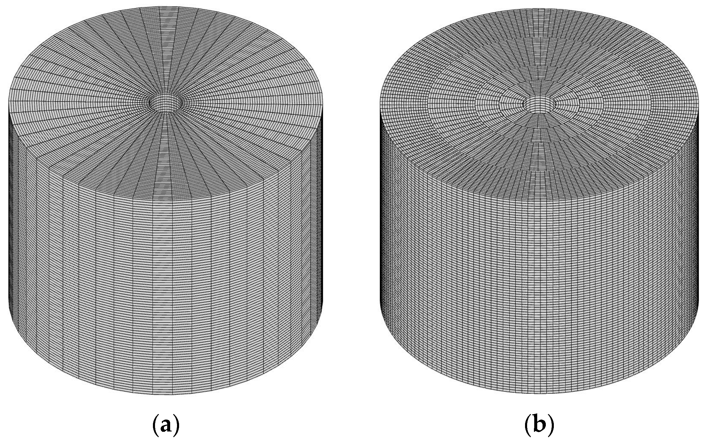
2.2. Grids Generation

In cylindrical coordinates, the azimuthal grid spacing differs from the center to the circumference, and the spacings are proportional to the radial distance in the implementation of the regular rectangular grid system (Figure 1a). The computation requires a small time step for the sake of numerical stability in cases of larger computational domains. To ensure grid-spacing independence and numerical stability, the zonal embedded grid technique proposed by Kravchenko et al. [38] and implemented by Suh and Yeo [39] is adopted in this study, as a larger-diameter wave tank is considered. In this system, the computational domain is partitioned into several blocks, with each block organized into a regular grid structure. A constant radial grid spacing is maintained in each block, and the azimuthal grid spacing can be adjusted independently block by block (Figure 1b). This approach enables significantly larger time steps compared to those possible with a regular orthogonal grid system.

2.3. Discretization of the Governing Equations

In the implementation of the zonal embedded grids within a cylindrical domain, the staggered grid arrangement introduced by Harlow and Welch [40] is used to address issues with differing grid interfaces in this wave tank model. According to this arrangement, velocities are placed on cell faces, while pressure, density, and viscosity are positioned in cell centers. The projection method introduced by Chorin [41] is adopted to couple the velocity and pressure fields, and the intermediate velocity $U^{\ast }$ is calculated using Equation (4), then, the velocities are projected into a divergence-free field using the Helmholtz–Hodge decomposition with Equation (5).

$$\begin{array}{c}{\displaystyle \frac{\left(m^n+C_A\left(1-m^n\right)\right)U^{\ast }-\left(m^n+C_A\left(1-m^n\right)\right)U^n}{\Delta t}}\\ =-{\left(u{\displaystyle \frac{\partial \left(mU\right)}{\partial r}}+{\displaystyle \frac{v}{r}}{\displaystyle \frac{\partial \left(mU\right)}{\partial \theta }}+w{\displaystyle \frac{\partial \left(mU\right)}{\partial z}}\right)}^n\\ +{\left({\displaystyle \frac{1}{r}}{\displaystyle \frac{\partial }{\partial r}} \left(\upsilon r{\displaystyle \frac{\partial \left(mU\right)}{\partial r}}\right)+{\displaystyle \frac{1}{r}}{\displaystyle \frac{\partial }{\partial \theta }} \left({\displaystyle \frac{\upsilon }{r}}{\displaystyle \frac{\partial \left(mU\right)}{\partial \theta }}\right)+{\displaystyle \frac{\partial }{\partial z}} \left(\upsilon {\displaystyle \frac{\partial \left(mU\right)}{\partial z}}\right)\right)}^n+S_U^n\end{array}$$

(4)

$$\begin{array}{c}{U}^{n+1}=U^{\ast }-{\displaystyle \frac{m^n}{{\rho }^n}}{\displaystyle \frac{\Delta t}{\left(m^{n+1}+C_A\left(1-m^{n+1}\right)\right)}}\nabla P^{\prime }; P^{\prime }=p^{n+1}{-p}^n\hfill \\ \nabla .U^{\ast }={\displaystyle \frac{m^{n+1}∆t}{\left(m^{n+1}+C_A\left(1-m^{n+1}\right)\right)}}\nabla .{\displaystyle \frac{1}{{\rho }^n}}\nabla \left(P^{\prime }\right)\hfill \end{array}$$

(5)

The high-resolution CICSAM (Compressive Interface Capturing Scheme for Arbitrary Meshes) method by Ubbink and Issa [42] is employed to accurately track fluid interfaces in the VOF convection equation. Additionally, a Jacobi-type dual-time-stepping scheme by Heyns et al. [43] is adopted to simplify computation and coding, enabling implicit approximation through an explicit formulation. The discretization of Equation (3) can be expressed as follows:

$$\begin{array}{c}m{\displaystyle \frac{F^{\tau +1}-F^{\tau }}{∆\tau }}+m{\displaystyle \frac{F^{\tau }-F^n}{∆t}}=Q\left(r_s,{\theta }_s,z,t\right)F^n\hfill \\ -{\displaystyle \frac{1}{2}}\left({\displaystyle \frac{1}{∆v}}\sum {flux{F}_f}^{\tau }m∆S+{\displaystyle \frac{1}{∆v}}\sum {flux{F}_f}^{n}m∆S\right)\hfill \end{array}$$

(6)

Here, $F_f^{\tau }$ and $F_f^n$ represent the volume fractions computed with the CICSAM scheme, $flux=\overrightarrow{U}\overrightarrow{n}$ denotes the mass flux, and $∆\tau$ is the pseudo-time step set to $2∆t/3$.

At each time step, the approximate velocity is initially calculated using Equation (4), followed by an evaluation of the pressure correction through the pressure Poisson equation (Equation (5)). The approximate velocity and pressure are then iteratively updated until the continuity (mass conservation) criterion is satisfied. Once the velocity has been updated, Equation (6) is employed to advect the air–water interface, and the whole procedure is iteratively repeated until the end of the computational time. The details of the discretized equations and computational procedures are explained in the appendix section (Appendix A).

3. Numerical Experiments

In this study, we used a wave tank with a diameter of about 10.2 m, and a wave maker with a diameter of 3 m was positioned in the center of the tank. The computational domain was subdivided into $5$ blocks, and grid arrangements in these blocks were $5\times 60\times 88$, $5\times 120\times 88$, $10\times 240\times 88$, $20\times 480\times 88$, and $80\times 960\times 88$ in radial, azimuthal, and vertical directions. The radial grid spacing was maintained at $\Delta r=0.03 \mathrm{m}$ in each block, while the grid spacings were set to 0.75 cm and 1.5 cm in the vertical direction here. To observe wave deformation and longshore current generation on a sandy sloping topography, the water surface elevation and velocity profiles were measured by setting the number of wave and velocity gauges at distance of 234 cm, 264 cm, 300 cm, 336 cm, 369 cm, and 405 cm from the center of the basin in each cross-section, as shown in Figure 2. The total circular domain was subdivided into 12 different cross-sections with 30° differences; a plain view of the cross-sections is shown in Figure 3. The computations were carried out for seven (07) individual cases (case 1 to case 7) corresponding to the wave periods ranging from T—1.25 s to T—2.50 s, respectively. The topography was set to a ratio of 1:7 to ensure that the wave transformation and breaking behavior were the same as those under typical natural beach conditions. The Courant–Friedrichs–Lewy (CFL) condition for time restriction was incorporated with a cell Courant number of less than 0.4 to ensure stability of the numerical algorithm and avoid oscillations during computation in this model. On the other hand, a no-slip boundary condition was implemented to ignore the reflection caused by the sidewall edges during spiral wave generation and propagation along the circular sloping topography. The computational conditions are summarized in

Table 1. Computation conditions for the numerical wave basin (cases 1–7).

Case	1	2	3	4	5	6	7
Period	1.25 s	1.50 s	1.60 s	1.82 s	2.0 s	2.22 s	2.50 s
Computation	60 s
Time	18 cm
Initial Terrain	1:7 Uniform Slope

.

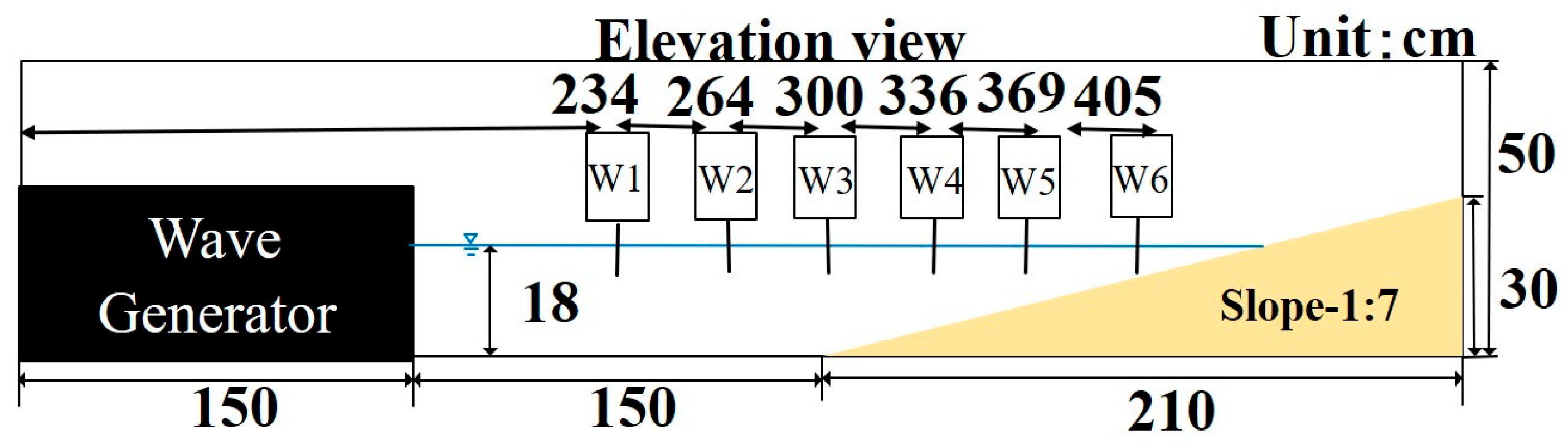
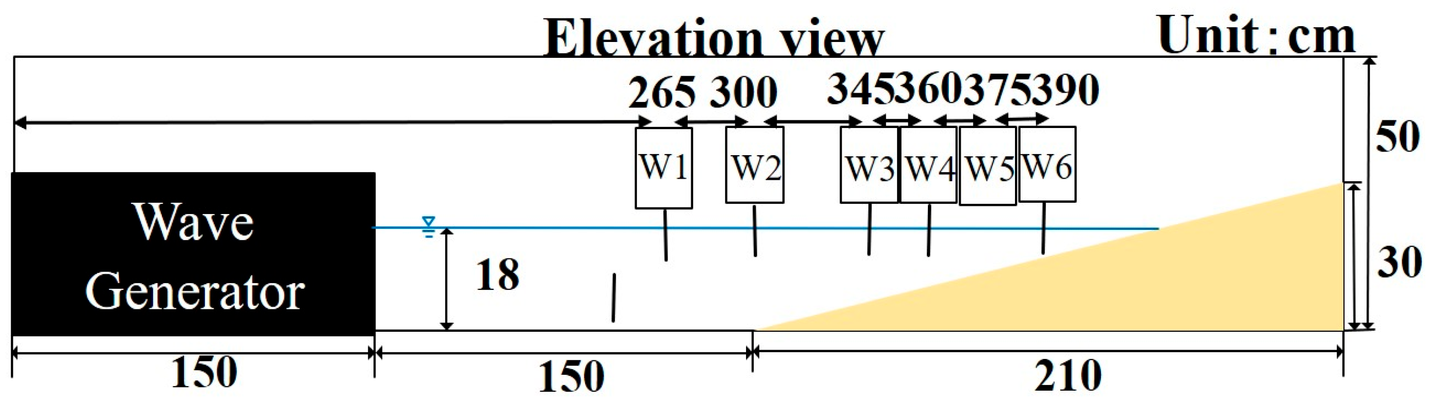
4. Outline of the Physical Experiment

To compare the computed results with the experimental results for validation, physical experiments were conducted in a basin with a diameter of 10.2 m with a 1:7 sandy beach slope, which were the same setting as applied in the numerical model. A non-rotational spiral wave maker with a diameter of 3 m was placed in the center of the wave basin. The physical experiments were performed at the Hydraulic Laboratory of Nagoya University, Japan, and the details of these experiments are explained in Islam et al. [30]. The computations were conducted with the same wave conditions in both the physical and numerical basin models; however, the physical experiments were conducted for 60 min per case, while the numerical simulations were conducted for 60 s. During the experiments, the wave gauges were set up in three different cross-sections (cross-section positions 1, 2, and 12 positions) with 22.5° differences to measure the water surface elevations. Six wave gauges (W1–W6) were set up at radial distances ranging from 265 cm to 390 cm from the center of the basin in cross-section 1, and four wave gauges were set up in cross-section 2 (W7–W10) and another four in cross-section 3 (W11–W14) at radial distances between 345 cm and 390 cm. The experiments were conducted for two wave period cases (T—1.82 s (case 8) and 2.22 s (case 9)) and a sectional view of the terrain (cross-section 1) along with the wave gauges’ positions is shown in Figure 4.

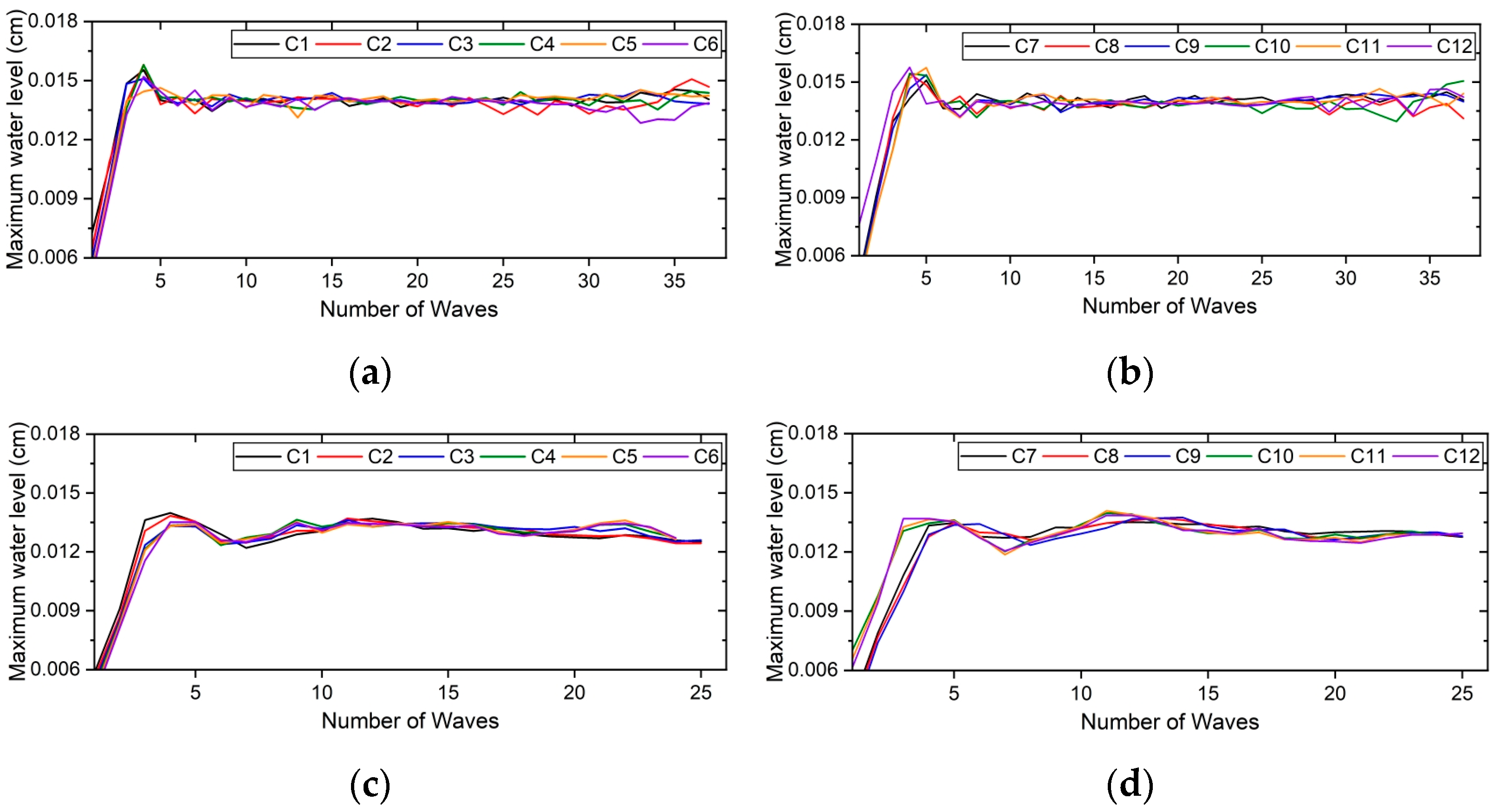
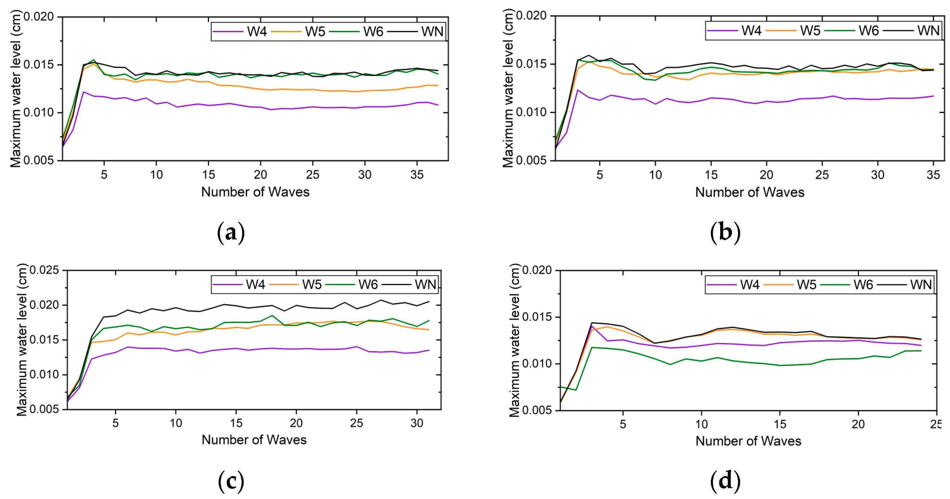
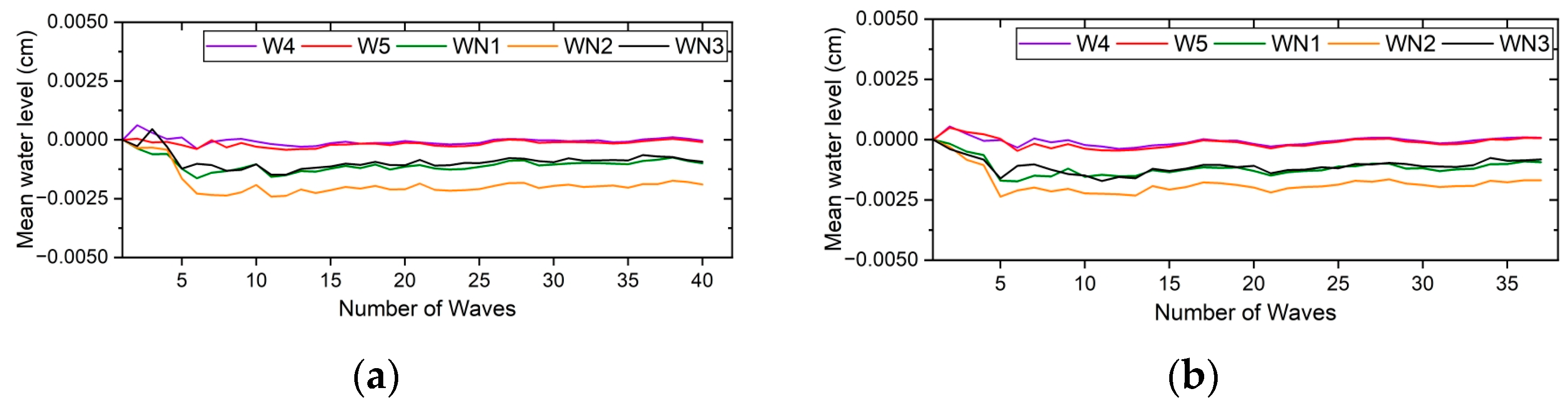
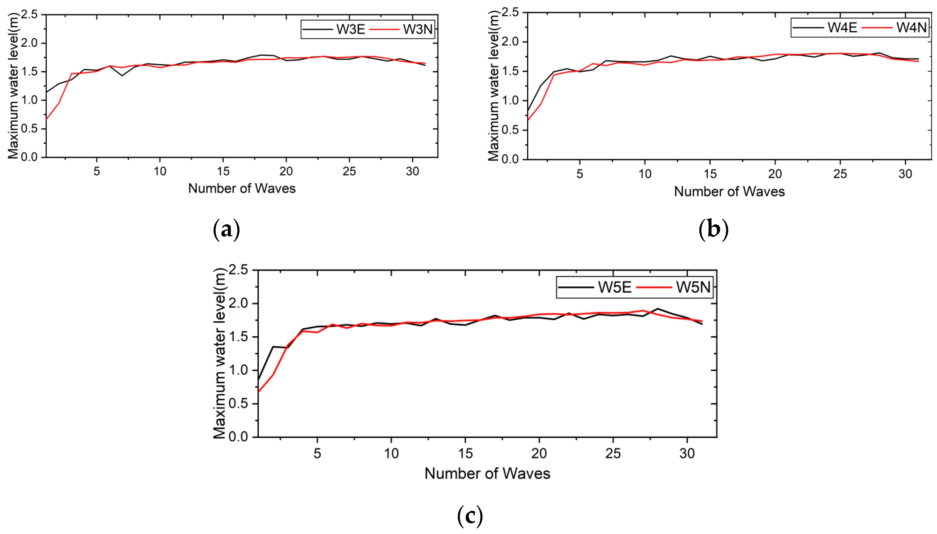
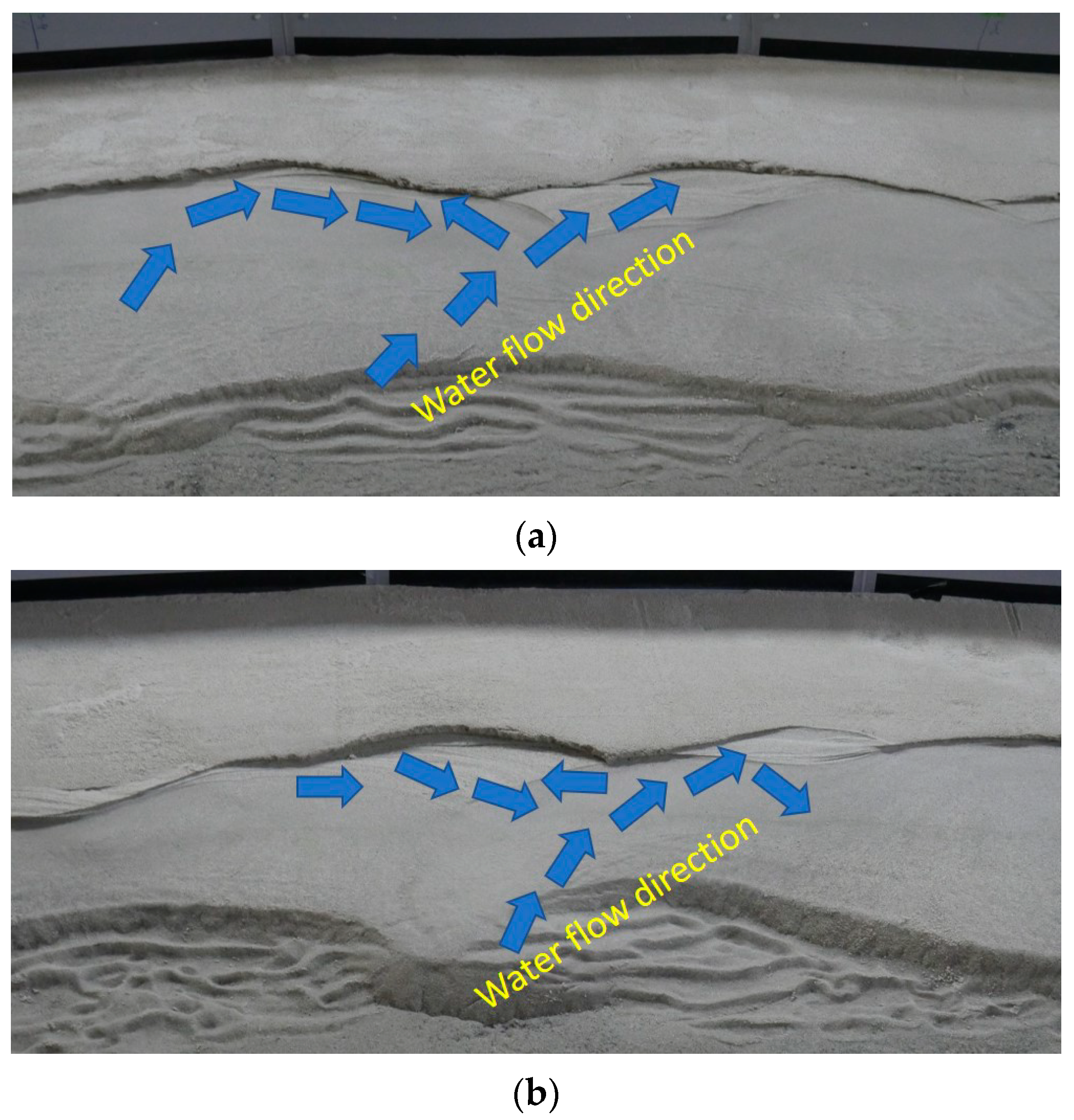
5. Results and Discussions

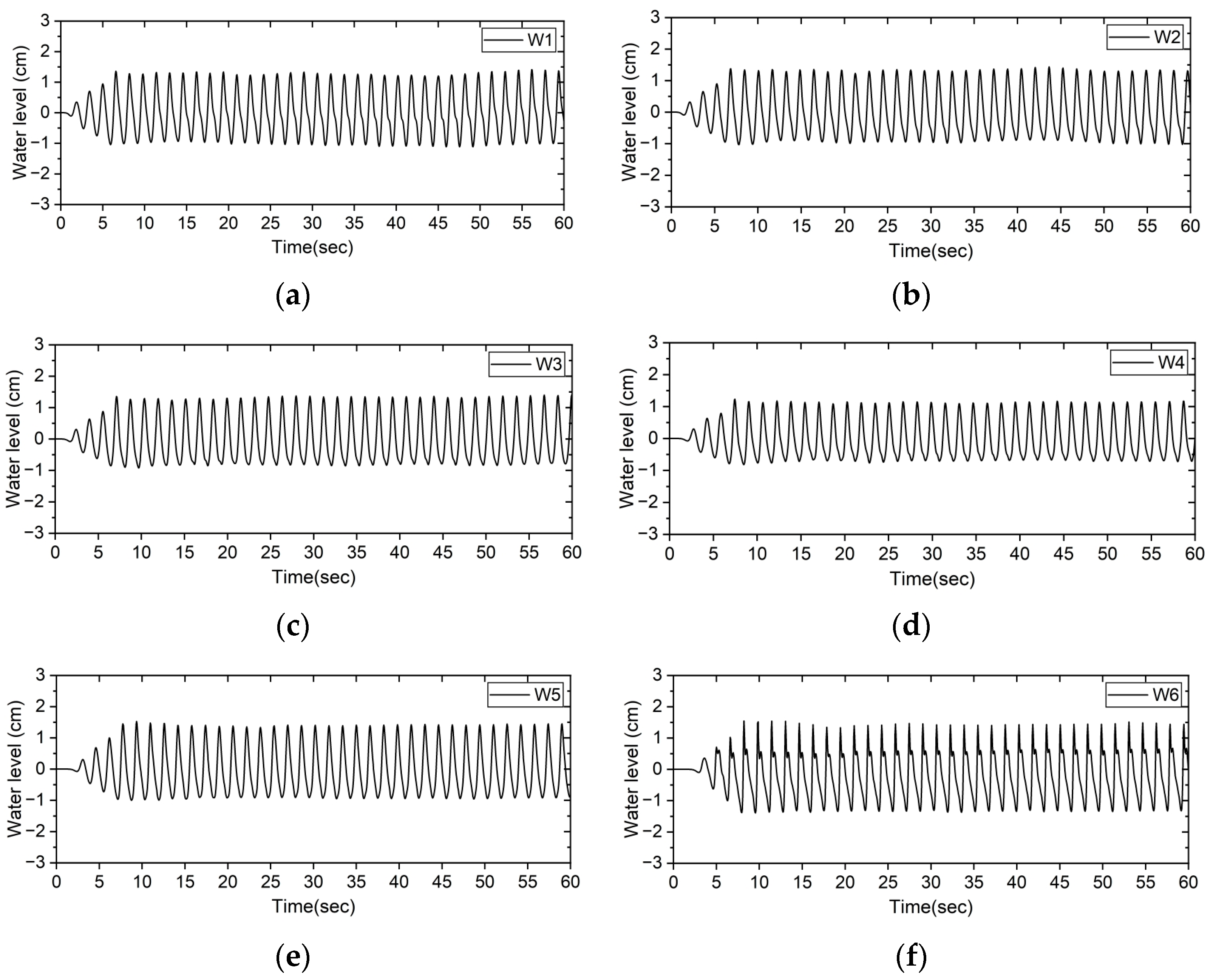
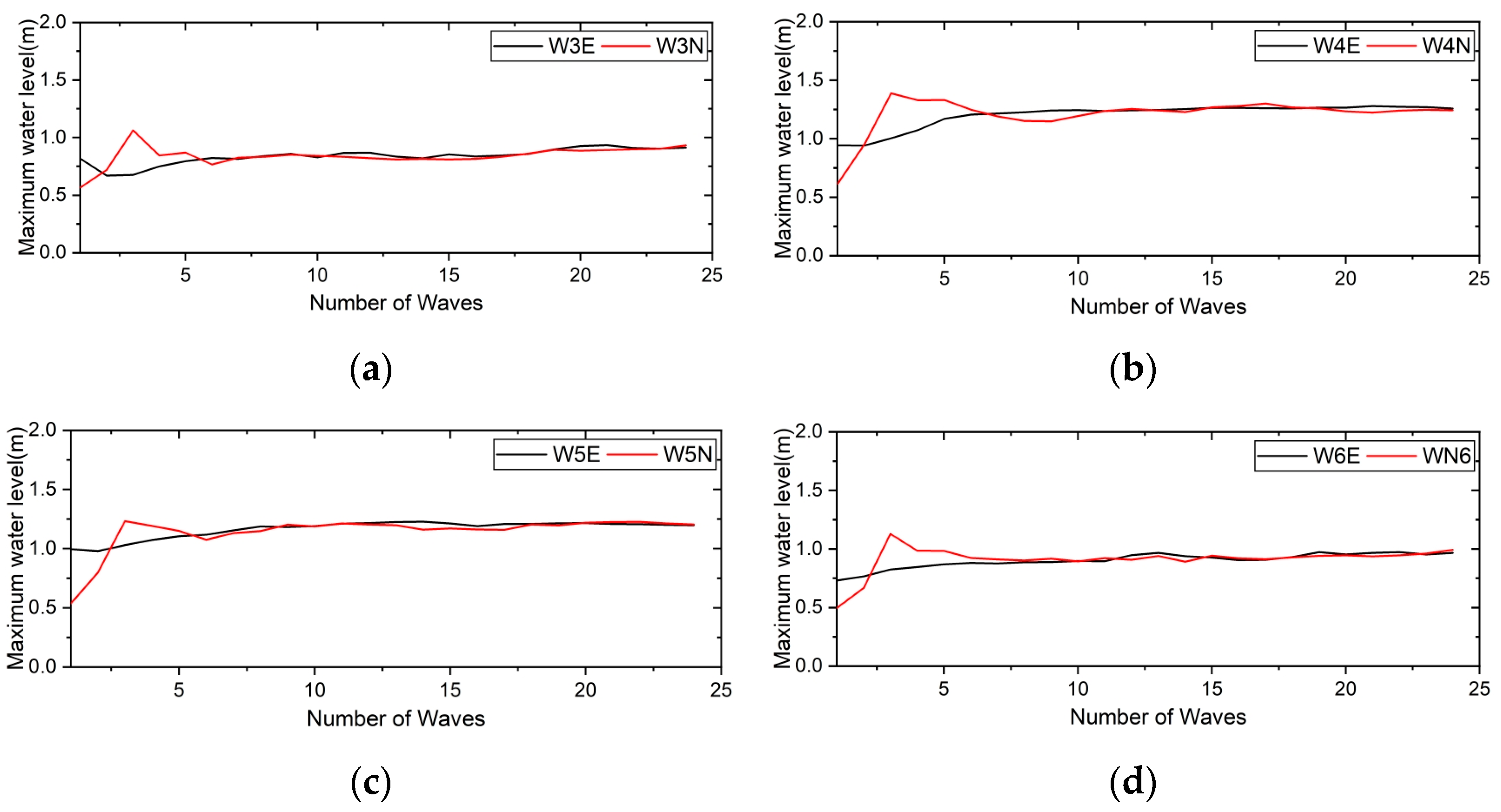
5.1. Characteristics of Water Surface Elevations

In this study, computations were performed for different wave conditions and water surface elevation profiles were measured to observe the wave deformation and other characteristics in different positions and cross-sections; and the measurement profiles are denoted by W1 to W6, as presented in Figure 2 and Table 1. From the computation, it was found that the water surface elevation magnitude gradually increased over time, and the values were mostly high at the wave gauges, positioned nearest the wave maker. In each case, surface elevation progressively decreased at wave gauges positioned farther from the wave maker, then increased again near the shoreline as a result of wave deformation and shoaling effects in shallow water. However, in some wave gauge positions, the wave heights did not consistently follow the above trends, and the wave heights decreased and increased at different wave gauge positions, whether close to or far from the center of the wave maker. In addition, it was found that the surface elevation magnitudes varied between wave period cases in the same measured position, and the magnitudes were higher in cases with high wave maker rotation speeds (number of rotations per minute) than in those with lower rotation speed, a similar trend to that found in [30]. However, the correlations of wave height variations with wave generator movement did not follow the above trends in all cases. These discrepancies could have occurred due to the influence of downstream flow and the incident-wave breaking around the measured position, as the length between the wave maker and the tank’s side wall and the water depth were fixed; in addition, sand displacement was not considered in this model in all wave condition cases. The differences in the surface elevation profiles can be seen in Figure 5 (case 3 (T—1.60 s)), where a still water level is represented by 0 cm, and the corresponding water surface elevations in cross-section 1 at wave gauges W1 to W6 are labeled accordingly.

Figure 5 shows that the water surface fluctuation magnitudes were higher at W1 and W2 than at W3 and W4, as W1 and W2 were closer to the wave maker, and the magnitudes increased again at W5 and W6, which were positioned nearest the shoreside; wave breaking could have occurred between the W5 and W6 due to the shallow water depth in this case. The magnitudes were high in most of the measured positions in case 1 (T—1.25 s), although some positions in individual cases showed an irregular tendency to increase and decrease. The wave period correlated with the movement of the wave generator, and there was faster movement in case 1 (T—1.25 s), which likely contributed to the increased surface elevations in the measured positions in the same angular cross-sections compared to the other wave condition cases. In some cases, the wave height variations did not follow the wave generator rotational speed trends mentioned above, with the magnitudes varied in the W4, W5, and W6 positions; the locations of incident-wave breaking could have been different in these cases. To determine the approximate wave-breaking positions and the deformation area in a single case, maximum water levels and mean water levels per wave were measured for all cases. The measurement profiles for cases 1 (T—1.25 s), 2 (T—1.50 s), 3 (T—1.60 s), and 6 (T—2.25 s) are shown in Figure 6. From this figure, it is clear that the maximum water levels per wave varied between wave condition cases, and individual values were higher from W4 to W6, and they differed between W4 and W6 in the same case. The profiles were significantly high at W6 in cases 1 and 2, were mostly high at W6 in case 3, varied between W5 and W6 in cases 4 and 5, were significantly high at W5 in case 6, and varied between W4 and W5 in case 7 in cross-section 1. On the other hand, the mean water levels were measured in the same positions and it was found that the values were lower in the above-mentioned positions. The measured profiles suggest that in general, the waves were breaking nearest to positions with higher maximum water levels, as well as the corresponding positions with lower mean water level magnitudes, in cases with a fixed sloping topography; these results are consistent with theoretical predictions of wave deformation in the surf zone on a sloping beach.

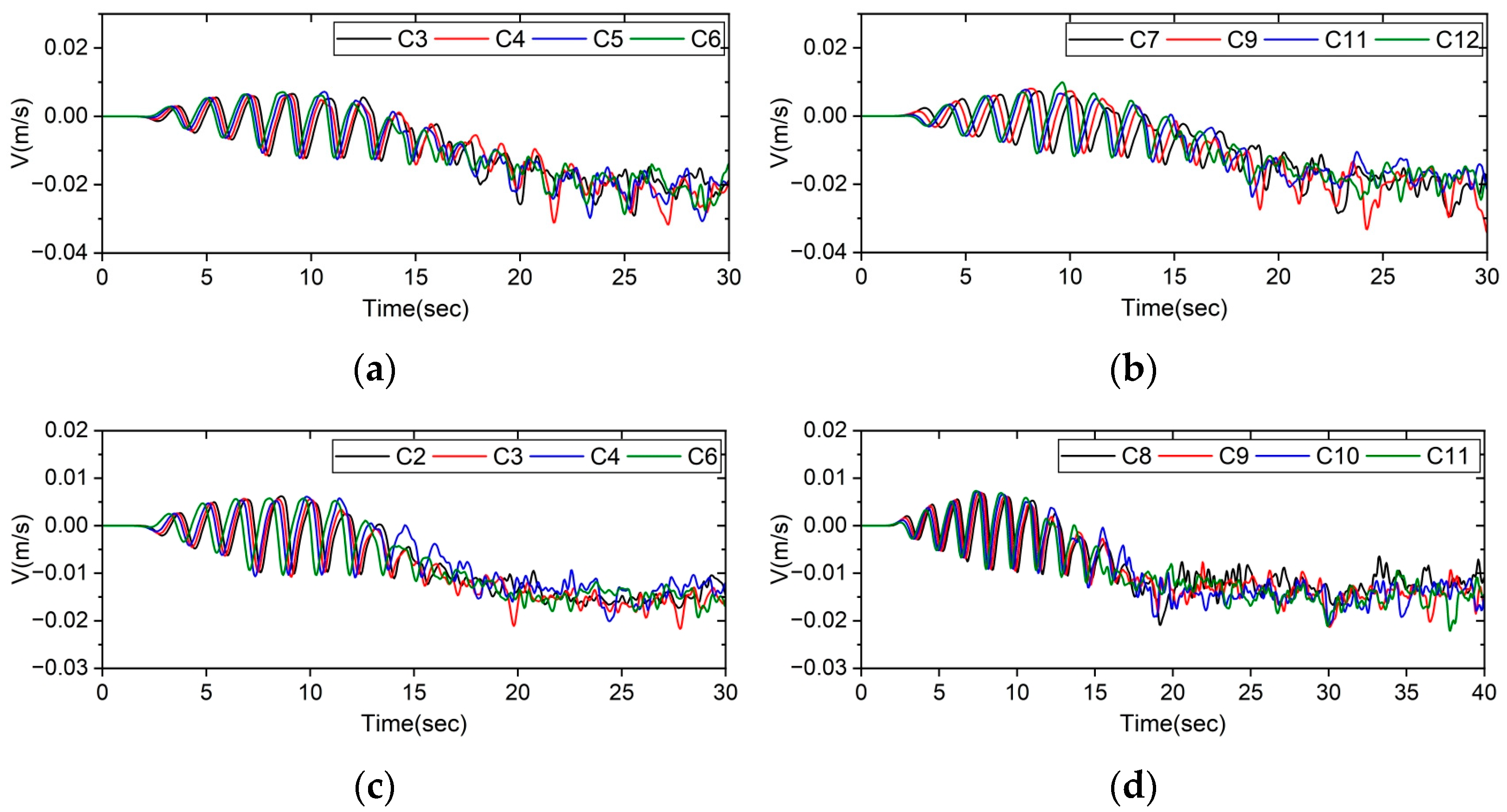
5.2. Comparisons Between Measured Cross-Sections

To observe the wave characteristic differences in individual cross-sections (Figure 3), measurements were conducted in each case, and we observed that the surface fluctuation profiles were mostly consistent in terms of magnitude at W1 (234 cm), W2 (264 cm), W3 (300 cm), and W4 (336 cm) in all measured cross-sections. The profiles varied considerably in terms of their crest and trough positions at W6 (405 cm), and varied a small amount at W5 (369 cm), in all cases; this discrepancy could be because the waves were moved towards the shore in a spiral-like and oblique manner and deformed in the shallow-water regions. The computed profiles in all measured wave gauges and cross-sections indicate that the considered wave source function effectively reproduced uniform spiral waves over the sloping beach.

From the computations of maximum water levels per wave in individual cross-sections, it was found that the magnitudes were high in the same radial positions, as observed in cross-section 1. However, the values varied in individual cross-sections in a single case, which can be observed in Figure 7, where the measured values in the radial positions of 405 cm and 369 cm in the 12 cross-sections for cases 2 and 6 are denoted by C1, C2,…, C12, respectively. These variations in the maximum water level profiles infer that the gradients of the water level could have been different, and that the generated waves did not fluctuate in a uniform manner during the swash and backwash processes in each cross-section. In addition, the wave-breaking positions, as well as the wave set-up, could have varied in the radial positions in the measured cross-section. A similar trend of wave-breaking position differences was found in the physical experiment, where the bar formation and wave-breaking positions were nearly coincident; the topography on the lower side was deformed with curve-shaped bars in individual cases in the different cross-sections, and a cusp-type topography was found in the T—1.82 s and T—2.0 s cases in [30].

To more accurately determine the approximated wave-breaking positions, water surface elevations were measured at each grid point between 309 cm and 414 cm in a single case, and we observed that the magnitudes of the maximum water levels were higher in the vicinity of 393 cm, 396 cm, 402 cm, 387 cm, 366 cm, and 351 cm for cases 1, 2, 3, 4, 6, and 7, respectively, and fluctuated between 369 cm (1–22 waves) and 402 cm (23–27 waves) for case 5. The computed results for cases 2, 3, 4, and 6 are shown in Figure 8, where WN defines the maximum water level measurement in the above-mentioned position in individual cases. Additionally, the magnitudes in the newly computed positions (WN) also fluctuated across cross-sections in individual cases, which indicates variation in the approximated wave-breaking positions in a single case, as described above.

In addition to the maximum water levels, the mean water levels were also computed in the above-mentioned positions (309 cm to 414 cm), and we found that the magnitudes were lower in the WN positions or nearest to the above-mentioned positions than in the other measured positions in a single case. Comparatively lower magnitude profiles were also found close to the WN position in some cross-sections; however, the distance of the lower-valued position was not as far as that of the assumed wave-breaking position in these cases. Comparisons of the mean water levels for cases 2 and 3 are shown in Figure 9, where WN1, WN2, and WN3 represent the computed mean water levels at 396 cm, 402 cm, and 411 cm, respectively, and lower values were found at 402 cm (WN2) in these two cases. The measurements of the mean and maximum water levels suggest that waves breaking occurred around the above-mentioned positions (WN) in an individual case. The wave set-up was also calculated in each cross-section, and we found that the maximum mean water levels were mostly high around 426 cm, and also varied between cross-sections. The variations in the positions with the lowest mean water level and the wave set-up profiles indicate that the downstream flows were not uniformly dominant and the wave run-up values could have varied at each cross-section in an individual case. The dominant properties of returning flow variations significantly influenced the variation in incident-wave breaking between cross-sections.

5.3. Model Validation

Although the results obtained by the presented model were previously validated by experiments conducted by Islam et al. [35], comparisons were made in only four different positions in one cross-section, so it was difficult to determine the wave-breaking positions from the experimental results. Physical experiments were conducted again for two cases (T—1.82 s, T—2.22 s) with 14 wave gauges to compare the outcomes against numerical simulations and to observe wave profiles in different measured positions, as well as the approximated breaking positions under the same wave conditions for validation. As topography deformation was not considered in the numerical model, the experimental data obtained before topography deformation was used for validation in this study. The wave profiles were measured with a closer distance than in Islam et al. [30], and we found that they followed a similar trend to those in the numerical experiments.

From the experimental outcomes, it was found that the water surface fluctuation profiles were mostly high in case 8 (T—1.82 s) at 375 cm and 390 cm, and in case 9 (T—2.22 s) at 360 cm and 375 cm, and were 387 cm and 366 cm in the numerical simulation. The maximum water levels were predominantly observed at 375 cm in cross-section 1 in case 8, whereas they were observed at 360 cm (W5) in case 9. In comparison to the other cross-sections, the maximum water levels were high, at 390 cm, in cross-sections 2 and 3 in case 8, and were mostly high, at 375 cm and 360 cm, respectively, in these two cross-sections in case 9. These results indicate that the waves were breaking between 375 cm and 390 cm; specifically, wave breaking mostly at 390 cm in case 8 and at 360 cm to 375 cm in case 9. In addition, the discrepancies in both water surface fluctuations and maximum-water-level positions indicate variations between cross-sections in the radial distance of the wave-breaking positions in these cases. The variations were identified from the topography photographs taken at the end of the experiments, where the bar positions were moved to the onshore or offshore side in different cross-sections in both cases. Comparisons of the maximum-water-level measurements in the same positions in both models are presented in Figure 10 and Figure 11. The experimental results were mostly consistent with those of the numerical simulations, but with a smaller difference. These discrepancies are likely attributable to sand displacement occurring in the physical experiments, which was not incorporated into the numerical wave basin model. From these comparisons, it can be deduced that the generated wave characteristics and the approximated wave-breaking positions were largely consistent in terms of radial distances in both wave tank models.

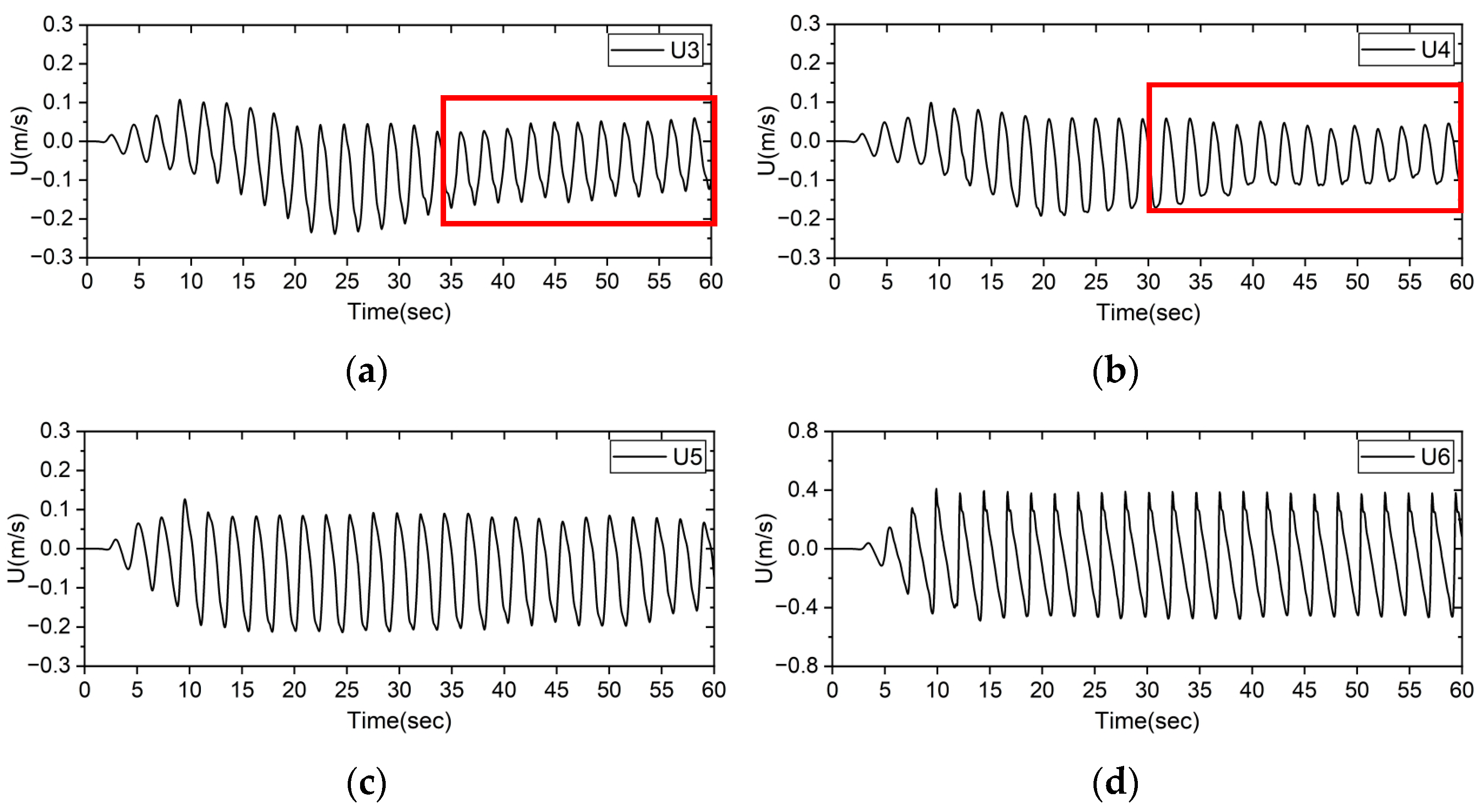
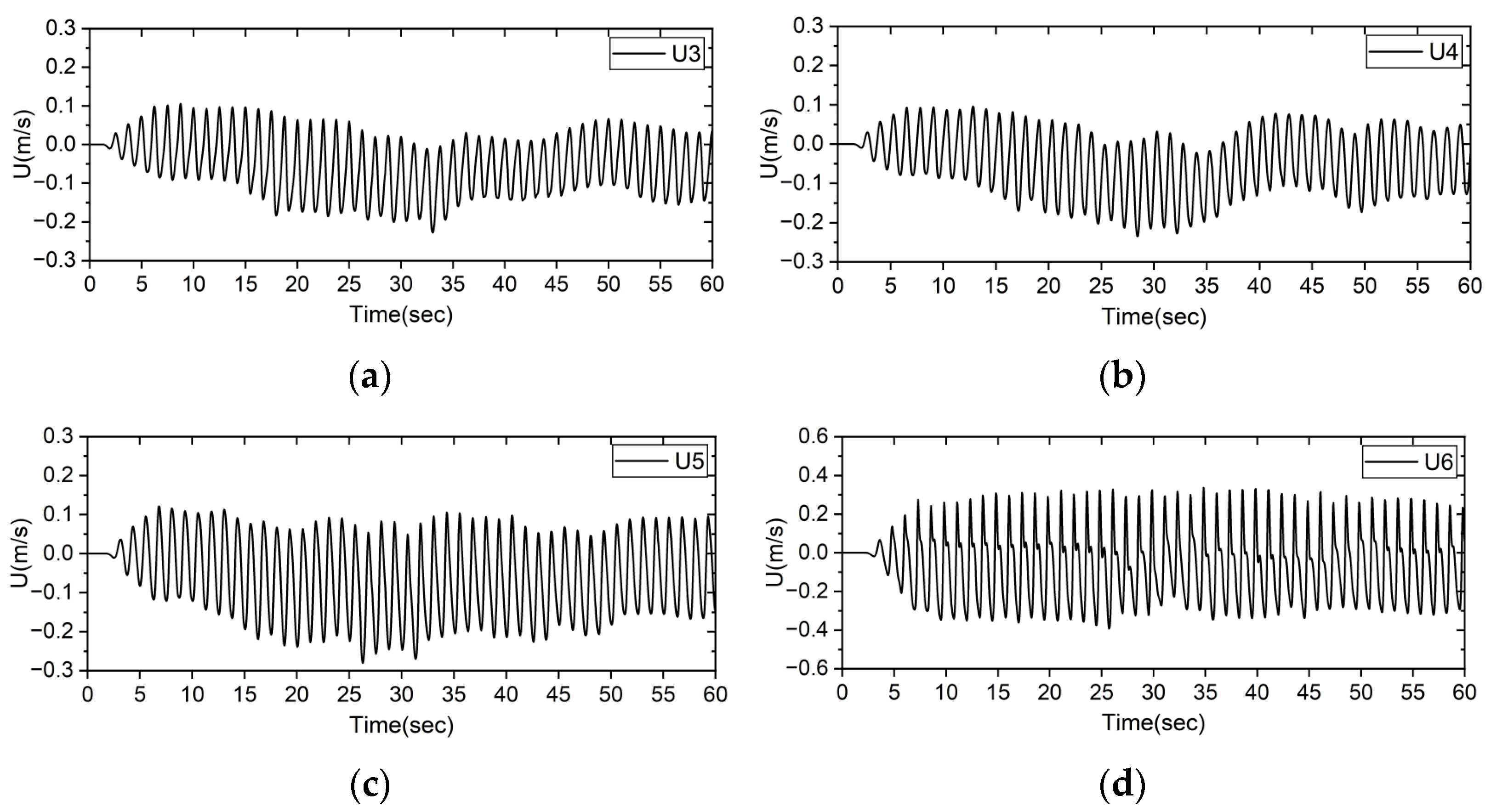
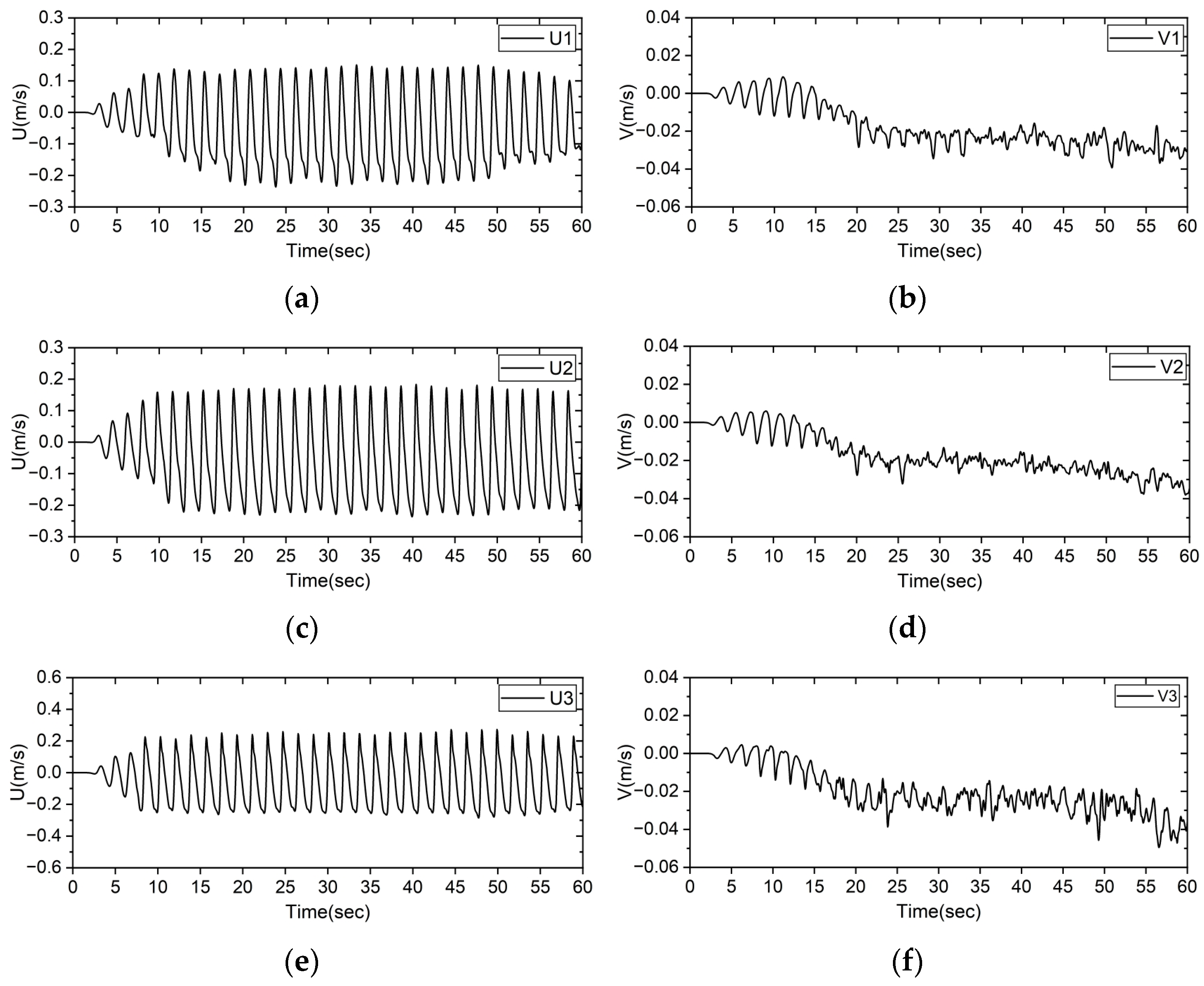
5.4. Cross-Shore Velocity Distribution

Velocity profiles in both the cross-shore and longshore directions were measured in positions corresponding to the wave gauges in all considered wave condition cases. Since the waves were breaking between approximately 351 cm and 402 cm as mentioned above, the velocity profiles were observed at 336 cm, 369 cm, and 405 cm to determine the probable area of longshore current generation in individual cases.

It was found that the cross-shore flow velocity profiles developed symmetrically from the start of the computation and gradually increased with time. The magnitudes were higher in cases where the wave maker’s rotational speed per minute was relatively higher. On the other hand, the magnitudes were higher at velocity gauges positioned on the sloping topography, and this was particularly significant for the gauges located close to wave-breaking positions to the shoreline in a single case. The velocity profiles did not follow the above trend in all measurement cross-sections in each case. The waves were deformed in the surf zone, and waters moved along the cross-shore direction according to the incident-wave breaking angle and upstream flow and returned rectangularly due to gravity and downstream flow, which could be the reason for the variations between measured positions. The computed velocity profiles for cases 3 and 6 are shown in Figure 12 and Figure 13, where the positive and negative values represent the onshore- and offshore-directed flow during computation.

The velocity profiles followed the cross-shore direction with little fluctuation at 234 cm and 264 cm; however, the upstream and downstream flows had little influence at these gauges, which were far from the shore line, in all cases. On the other hand, the profiles moved symmetrically from the beginning of the calculation from a position of 300 cm and to other positions in all cases; in this study, this trend is defined as the dominant cross-shore velocity characteristic. Eventually, they moved downward with little fluctuation, and then moved by approximately the same amount between the crest and trough positions until the end of the computation, which is defined in this study as stable cross-shore velocity formation. The stable velocity profile formation was more significant at 336 cm and 369 cm in all cases, whereas the computed profiles moved stably or in small upward–downward motions (red box) between the crest and trough positions in some cases at 300 cm. The velocity profiles were mostly stable, with high magnitudes at 405 cm from the start of computation, in all cases. In some cases, stable cross-shore velocity was found for a few waves; then, the trough positions moved upward, whereas the crest positions were comparatively stable at 336 cm and 369 cm. Notably this trend was found in cases 5, 6 (Figure 13, red boxes), and 7, respectively. Since the waves were approximately breaking between 336 cm and 414 cm, as explained in the previous section, the upstream flow could be moved significantly along the onshore directions; however, the returning flow moved slowly or opposite to the rotational direction so that the trough positions moved to upward and the magnitudes of the velocity profiles decreased in a single case. Additionally, the duration of the run-up and run-down processes could have been different from the actual wave period in these cases.

From the comparisons in individual cases, it was found that the stable velocity profiles exhibited little fluctuation after 25 s for cases 2 and 3, and after approximately 22 s in cases 4 and 5. On the other hand, upward movement of the trough positions was found between 36 and 42 s in cases 5 and 6, after which it remained relatively stable until the end. At U5, the velocity profiles moved stably with little fluctuation after 18 s in cases 2 and 3, and after 15 s in case 4. This stable trend was observed between 15 s and 38 s at U5 in case 5; then, the trough positions exhibited small fluctuations until the end. Significant stable cross-shore velocity was found after 18 s in cases 6 and 7, and this stable trend continued until the end. The velocity profiles were mostly stable at U6 from the start of computation in all cases except case 1; these stable profiles are shown in Figure 12d and Figure 13d, respectively. The time that elapsed prior to stable velocity profile formation at U4 and U5 indicates that the cross-shore velocity was dominant until the above-mentioned time periods in individual cases. On the other hand, the velocity profile characteristics were different in case 1 (T—1.25 s), with too many fluctuations; in this case, the upstream flow could have been moved in the opposite direction to the rotation, and the wave period might have been different in the swash area than the considered wave period (T—1.25 s) (Figure 14). The above-mentioned velocity profile characteristics were also found in the 12 measured cross-sections in each wave condition case.

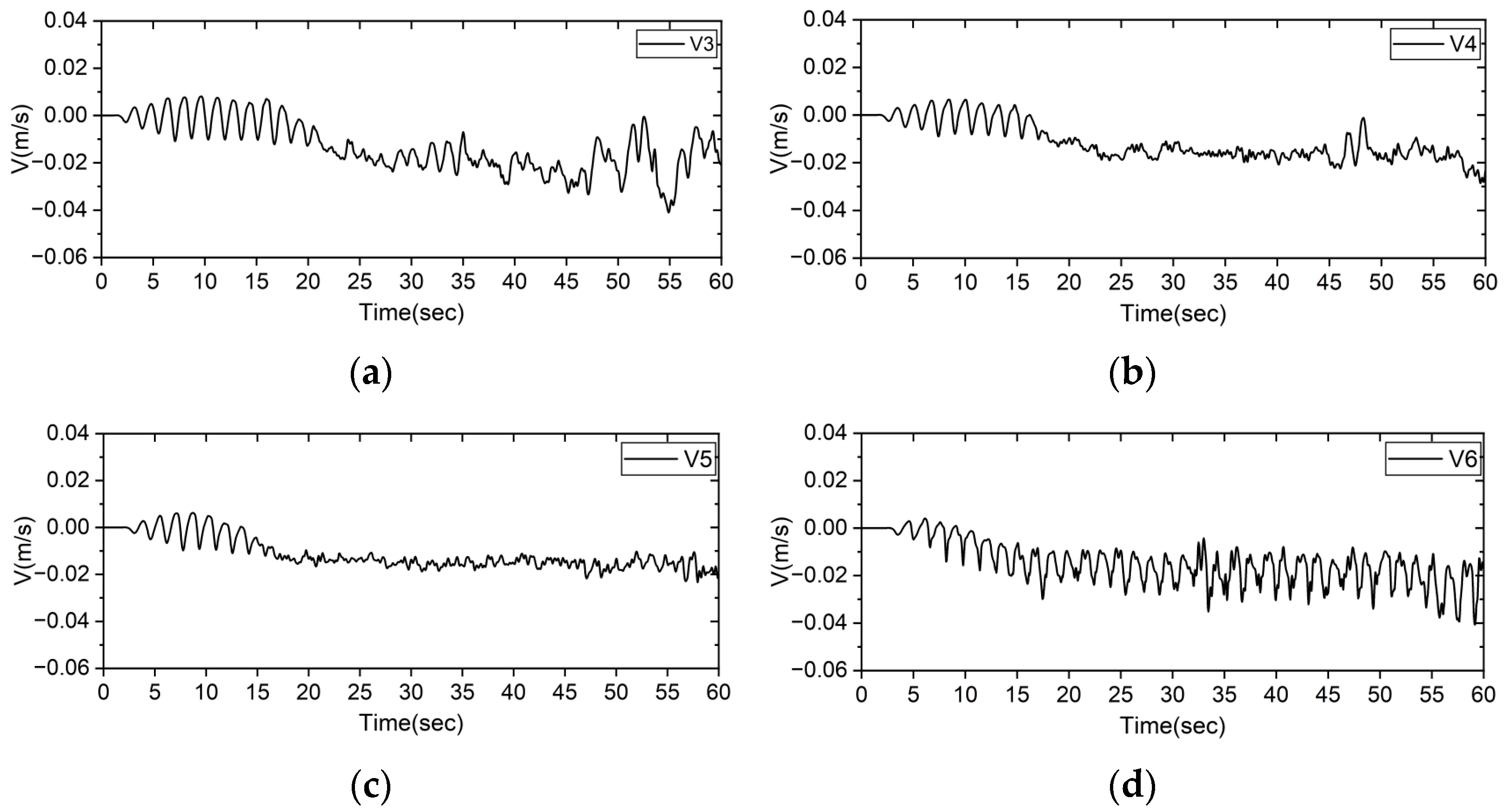
5.5. Longshore Velocity Distribution

The longshore flow velocity ($V$) was nearly symmetrical from the start of computation, and the flow velocities moved in the corresponding and opposite directions to the rotation of the wave maker in all cases. The velocity profiles for case 3 are shown in Figure 15. The negative magnitudes of the profile define the flow movement along the direction of rotation, while the positive magnitudes define movement in the opposite direction. From the computations, it was observed that the flow velocity magnitudes gradually increased and were symmetrical for a few seconds, then followed the alongshore direction in all cases at V1 to V5. This trend of alongshore-directed flow movement with negative magnitudes is defined as the dominant longshore velocity characteristic in this study. The flow velocity was more dominant at V3 to V6 than at V1 to V2 in all cases. Remarkably, movement in the opposite direction to rotation was observed in case 1, while the dominant characteristic was found at V4 and V5 in cases 2 to 6. Since the generated wave heights gradually increased as the wave maker’s rotation speed increased, and the adopted beach slope (1:7) was steep enough in this model, the generated waves could have moved too fast in case 1, and the returning flows moved in the opposite direction to rotation. The flow velocity movement in the alongshore direction was not significant in any measured position in case 7, as also observed in the previous cases. As the wave maker’s speed was lower in this case, the downstream flow could have been less dominant than the upstream flow, which is evident from the velocity computation and videos recorded during the physical experiment.

In the individual computations, it was found that the longshore flow velocity was more significant after 22 s and 18 s in the V4 and V5 positions in case 2, and the durations were mostly the same, with stable cross-shore velocity distribution at U4 and U5. Alongshore-directed dominant velocity profiles with too much fluctuation were more prominent from the beginning of the simulation at V6; however, in this case, velocity components moving in the opposite direction were found at V1 to V3. A similar velocity profile trend to that in case 2 was found in all measured positions in cases 3, 4, and 5; however, the starting point of periods of longshore velocity dominance varied in these cases, and periods of stable cross-shore velocity distribution were concentrated at U4 and U5, as observed in case 2. Alongshore-directed flow velocity with mostly the same magnitudes and minimal fluctuations were observed at V5 (Figure 15c) in case 3 and V4 in cases 4 and 5, with V5 and V4 usually defined as areas of strong longshore velocity dominance in these cases. The longshore flow velocity followed the same trend at V4 in case 6; however, the velocity profiles fluctuated after 45 s (Figure 16c, red box), which could have occurred because the downstream flow was weak and moved in the opposite direction. The longshore flow velocity was more notable in case 5 than in case 6, with smaller fluctuation at V5 than in the other positions; meanwhile, the velocity profiles fluctuated at V4 after 45 s (Figure 16c, red box), which could have occurred because the downstream flow movement was weaker and moved in the opposite direction in this case. The velocity profiles fluctuated at the same, and the flow moved in the opposite directions to the rotation of the wave maker, in all measured positions in case 1, and the fluctuations were significant from V4 to V6, as shown in Figure 16a,b. The above-mentioned characteristics of longshore velocity distribution were observed in cross-section 1, with small variations in all 12 cross-sections in each case; this is clear from the comparisons of the velocity profiles of velocity gauges in position V5 at similar distances from the center of the basin in eight random cross-sections for cases 3 and 4, where C2, C3,… represent the cross-section numbers as shown in Figure 17.

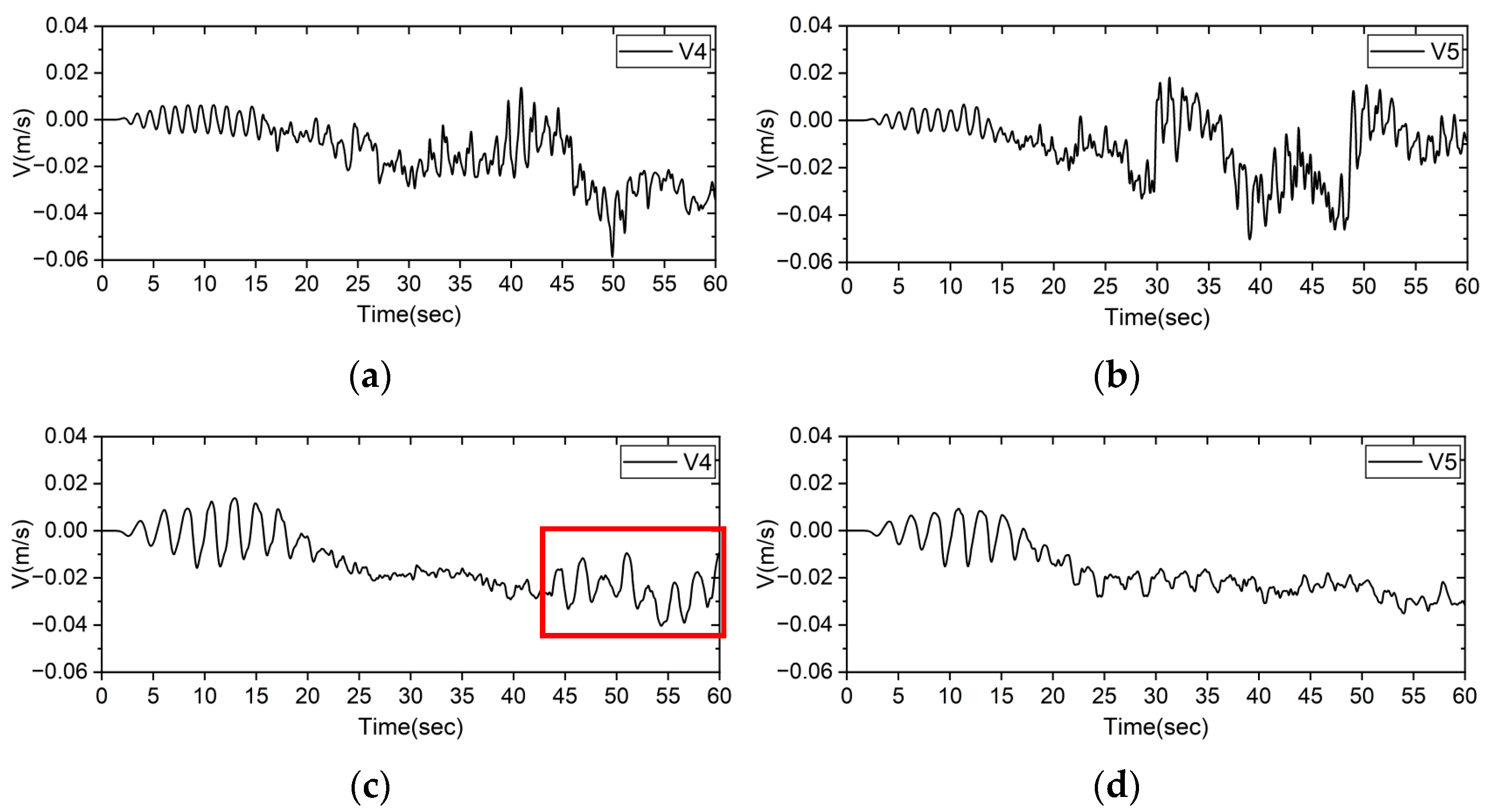
5.6. Longshore Current Generation

To more accurately determine the probable longshore current generation and generation area in the present wave tank model, the cross-shore- and longshore-directed velocities were measured again between 309 cm and 414 cm in 12 cross-sections. We focused on the positions of the stable cross-shore velocity profile formations as well as the smaller fluctuating longshore velocity profiles in accordance with the direction of rotation. If the velocity profiles in both directions followed the above-mentioned procedures in the same positions nearest the wave-breaking areas in an individual case, it would be concluded that the longshore current might have been formed adjacent to the measured zone in that case. A comparison of the velocity profiles of the cross-shore- and longshore-directed measurements before the approximated wave-breaking positions, at the approximated positions, and after the presumed longshore current generation area, are shown in Figure 18 and Figure 19 for cases 3 and 4, respectively.

From the computation, it was found that the cross-shore velocity profiles were approximately stable in the crest and trough positions between 381 cm and 390 cm 16–18 s after the random measurement of velocity gauges, and continued until the end of the computation, in case 2. Before this time period (16–18 s), cross-shore velocities were dominant and followed the rotational movement of the wave maker in all 12 cross-sections. On the other hand, the longshore velocity profiles moved symmetrically between 381 cm and 390 cm from the start of computation until 16–18 s; after that, the profiles moved more significantly in the alongshore direction with a small amount of fluctuation over time compared to the other measured positions. The cross-shore velocity profiles were found to be remarkably stable in all measured positions between 396 cm and 414 cm; however, the longshore velocity profiles fluctuated too much at the above-mentioned distances. Since the approximated wave-breaking positions were in the vicinity of 396 cm in this case, the fluids could move towards the upper side of the shore throughout the dissipated wave energy and return in the offshore direction due to gravity. Thus, the fluid velocity components in the cross-shore direction were moved stably; however, in this case, the longshore-directed components fluctuated in these measured positions (396 cm to 414 cm) due to the significant influence of downstream flow, as shown by the velocity profiles. As the maximum water levels were higher and the mean water levels lower in case 2 than in the other cases nearest 396 cm, the velocity profiles in the cross-shore and longshore directions were also stable and followed the above-mentioned process, so it is possible that the longshore current was generated between 381 cm and 390 cm in case 2. Similar velocity profile trends in both the cross-shore and longshore directions with smaller fluctuations were observed from 384 cm to 393 cm in case 3; however, the velocity profile magnitudes varied slightly more in this case than in case 2. From the measurement of the velocity profiles before and after the approximated wave-breaking positions (402 cm), it is possible that a longshore current was generated between 384 cm and 393 cm in case 3 (Figure 18). In case 4, stable cross-shore velocity profiles that exhibit dominant longshore velocities with small fluctuations were found between 372 cm and 381 cm in all measured cross-sections. In some cross-sections, longshore velocity profiles were significant between 363 cm and 375 cm, although the cross-shore velocity profiles were relatively stable during the early stage of the simulation. The influence of downstream flow movement could have been different in individual cross-sections, which could be one reason for the generation of these profiles. The velocity profile variation before and after the approximated wave-breaking positions is shown in Figure 19. The area of longshore current generation area could have varied between cross-sections in this case.

In some cross-sections of case 5, the profiles were found to be similar to those in case 4 between 354 cm and 363 cm, and stable cross-shore velocity profiles, along with dominant longshore velocity movement, were observed between 378 cm and 390 cm, but not for the previously measured distances (354 cm to 363 cm). Since the approximated wave-breaking positions (based on the maximum and mean water level measurements) varied from 369 cm to 402 cm in different cross-sections in this case, the influence of downstream flows was not uniform in each cross-section. In the physical experiment, it was visually observed that the upwelling positions of the incoming waves differed over time between cross-sections, and the upstream flow movement was in the opposite direction; the shape of the upper topography was changed to a U-shape. The bar positions were found to be far from the shoreline in the offshore direction or somewhere close to the shoreline, forming concave and convex shapes, unlike the other areas around the circular beach topography; this is shown in Figure 20. In the physical experiments, the upwelling positions were transformed as a result of longshore current generation and the interaction between upstream and downstream flows across various cross-sections. Based on the velocity profile measurements in the numerical wave basin model, it is possible that the longshore current generation positions were transformed in the vicinity of 360 cm to 387 cm in different cross-sections. This spatial variation appeared to be influenced by the combined effects of upstream and downstream flow movement in both the same and the opposite direction to the wave maker’s rotation during the computation time, which was also observed in the physical experiments.

The velocity profiles in both directions for possible longshore current generation were observed between 357 cm and 363 cm and continued after 363 cm in case 6. However, the longshore velocity profiles fluctuated, and the trough and crest positions in the cross-shore profiles of the different cross-sections also fluctuated between distances of 348 cm and 363 cm. The longshore current generation areas were not more prominent in case 6 than in cases 2 to 5, as shown in Figure 21. In case 7, the crest and trough positions of the cross-shore velocity profiles were stable for a short duration and then fluctuated in all measured cross-sections. Additionally, the longshore velocity profiles fluctuated too much, and no profiles were found to exhibit small amounts of fluctuation in the vicinity of the approximated wave-breaking positions. On the other hand, the longshore velocity profiles fluctuated too much without exhibiting any significant characteristics in case 1, and the velocity profiles in both the cross-shore and longshore directions fluctuated in all of the measured cross-sections; moreover, the longshore velocity was found to exhibit a significant zig-zag pattern, as shown in Figure 14 and Figure 17. Thus, the generation of longshore currents in case 1 seems to be difficult under the given wave and sloping conditions.

From the above discussion, it can be inferred that the directions of upstream and downstream flow movement significantly influenced the velocity distributions, and the influence of the downstream flow in the alongshore direction should be minimal nearest the wave-breaking positions to model a longshore current generation area on sloping topography (Li and Johns [8]; Visser [21]). Longshore current generation likely acted as a wave-driving force during periods of stable cross-shore velocity and significant longshore velocity, with minimal fluctuation measured in these areas in the presented wave tank, and was considered to be the reason for the beach profile deformation during the experiments in the physical circular wave tank. In addition, the combined relationships between the wave-breaking positions, dominant-returning-flow zones with smaller fluctuations in various wave period cases, and the sloping topography were responsible for the generation of the longshore current in the sloping beach topography, as demonstrated in the presented numerical wave tank model.

6. Conclusions

A circular wave basin model with a permeable sloping beach (1:7) was introduced to identify the wave deformation and longshore current generation zones, which are analogous to those occurring along natural sandy beach profiles. The numerical results were validated against experimental data, demonstrating good agreement in randomly selected water surface elevation profiles under the same wave periods and slope conditions in both the numerical and physical models. The maximum water level per wave was consistently higher near the estimated wave-breaking positions within individual cross-sections, while the mean water level remained lower in adjacent areas of the numerical basin model. However, these two profiles varied between cases, and even among cross-sections within the same case, indicating a potential correlation with wave period and the associated wave-breaking positions occurring at similar radial distances. The cross-shore velocity profiles were significant from the starting point of the computations and then eventually became relatively stable. In addition, the longshore velocity profiles followed the alongshore direction, with smaller fluctuations, under the same durations and in the same measured positions nearest the wave-breaking positions in different cross-sections. The presence of stable velocity profiles, coupled with minimal influence of downstream flow adjacent to the approximated wave-breaking positions, allowed us to infer that there could be zones of longshore current generation over the sloping topography that moved in a parallel manner in the alongshore direction in the numerical wave basin model. The computation results indicated a relationship with the incident-wave-breaking positions, the velocity distribution, and the influence of the downstream flow on probable longshore current generation on a sloping beach. Although the computed results showed good agreement with the experimental results, we did not compare the errors in the water level variations in the numerical and experimental cases in this study, which may be considered in future research. In addition, the turbulence and sand displacement terms were not considered in this study; in future work, these can be included to explain the processes of longshore sediment transport and beach deformation on a sandy natural beach through experiments and observation on a natural beach. In future research, the presented model can be modified to comprehensively investigate the influence of incident-wave breaking and sediment impact on longshore current generation under varying wave and slope conditions.

References

1. Guza, R.T.; Thornton, E.B. Wave set-up on a natural beach. J. Geophys. Res. 1981, 86, 4133–4137. [Google Scholar] [CrossRef]
2. Allard, R.; Rogers, E.; Martin, P.; Jensen, T.; Chu, P.; Campbell, T.; Dykes, J.; Smith, T.; Choi, J.; Gravois, U. The US navy coupled ocean-wave prediction system. Ocean 2014, 27, 93–103. [Google Scholar] [CrossRef]
3. Battjes, J.A. Modeling of turbulence in the surf zone. In Proceedings of the A Symposium Focused on Modeling Techniques, San Francisco, CA, USA, 3–5 September 1975; ASCE: Reston, VA, USA, 1975; pp. 1050–1061. [Google Scholar]
4. Davidson-Arnott, R.G.D.; McDonald, R.A. Nearshore water motion and mean flows in a multiple parallel bar system. Mar. Geol. 1989, 86, 321–338. [Google Scholar] [CrossRef]
5. Svendsen, I.A.; Putrevu, V. Nearshore mixing and dispersion. Proc. R. Soc. Lond. Ser. A Math. Phys. Sci. 1994, 445, 561–576. [Google Scholar]
6. Fredsoe, J.; Deigaard, R. Mechanics of Coastal Sediment Transport; World Scientific: Singapore, 1992; p. 369. [Google Scholar]
7. Li, Z.; Johns, B. A three-dimensional numerical model of surface waves in the surf zone and longshore current generation over a plane beach. Estuar. Coast. Shelf Sci. 1998, 47, 395–413. [Google Scholar] [CrossRef]
8. Bever, A.J.; MacWilliams, M.L. Simulating sediment transport processes in San Pablo Bay using coupled hydrodynamic, wave, and sediment transport models. Mar. Geol. 2013, 345, 235–253. [Google Scholar] [CrossRef]
9. Bowen, A.J. The generation of longshore currents on a plane beach. J. Mar. Res. 1969, 27, 206–215. [Google Scholar]
10. Longuet-Higgins, M.S. Longshore currents generated by obliquely incident sea waves, 1. J. Geophys. Res. 1970, 75, 6778–6789. [Google Scholar] [CrossRef]
11. Longuet-Higgins, M.S. Longshore currents generated by obliquely incident sea waves, 2. J. Geophys. Res. 1970, 75, 6790–6801. [Google Scholar] [CrossRef]
12. Thornton, E.B. Variation of longshore current across the surf zone. In Proceedings of the 12th International Conference on Coastal Engineering, Washington, DC, USA, 13–18 September 1970; American Society of Civil Engineers: Reston, VA, USA, 1970; pp. 291–308. [Google Scholar]
13. Thornton, E.B.; Guza, R.T. Surf zone longshore currents and random waves: Field data and models. J. Phys. Oceanogr. 1986, 16, 1165–1178. [Google Scholar] [CrossRef]
14. Komar, P.D.; Inman, D.L. Longshore sand transport on beaches. J. Geophys. Res. 1970, 75, 5914–5927. [Google Scholar] [CrossRef]
15. Bayram, A.; Larson, M.; Hanson, H. A new formula for the total longshore sediment transport rate. Coast. Eng. 2007, 54, 700–710. [Google Scholar] [CrossRef]
16. Van Rijn, L.C. Unified view of sediment transport by currents and waves I: Initiation of motion, bed roughness and bed-load transport. J. Hydraul. Eng. 2007, 133, 649–667. [Google Scholar] [CrossRef]
17. Van Rijn, L.C. Unified view of sediment transport by currents and waves II: Suspended transport. J. Hydraul. Eng. 2007, 133, 668–689. [Google Scholar] [CrossRef]
18. Kraus, N.C.; Sasaki, T.O. Effects of wave angle and lateral mixing on the longshore current. Coast. Eng. Jpn. 1979, 22, 59–74. [Google Scholar] [CrossRef]
19. Visser, P.J. Uniform longshore current measurement and calculations. In Proceedings of the 19th Conference on Coastal Engineering, Houston, TX, USA, 29 January 1984; pp. 2192–2207. [Google Scholar]
20. Visser, P.J. A mathematical model of uniform longshore currents and the comparison with laboratory data. In Communications on Hydraulic Engineering; Report/Department of Civil Engineering, Delft University of Technology: Delft, The Netherlands, 1984; p. 151. [Google Scholar]
21. Visser, P.J. Laboratory measurements of uniform longshore currents. Coast. Eng. 1991, 15, 563–593. [Google Scholar] [CrossRef]
22. Johns, B.; Jefferson, R.J. The numerical modeling of surface wave propagation in the surf zone. J. Phys. Oceanogr. 1980, 10, 1061–1069. [Google Scholar] [CrossRef]
23. Hamilton, D.G.; Ebersole, B.A. Establishing uniform longshore currents in a large-scale sediment transport facility. Coast. Eng. 2001, 42, 199–218. [Google Scholar] [CrossRef]
24. Kobayashi, N.; Lawrence, A.R. Cross-shore sediment transport under breaking solitary waves. J. Geophys. Res. Ocean. 2004, 109, C03047. [Google Scholar] [CrossRef]
25. Liangduo, S.; Qinqin, G.; Zhili, Z.; Lulu, H.; Wei, C.; Mingtao, J. Experimental study and numerical simulation of mean longshore current for mild slope. Wave Motion 2020, 99, 102651. [Google Scholar] [CrossRef]
26. Dalrymple, R.A.; Dean, R.G. The spiral wavemaker for littoral drift studies. In Proceedings of the 13th International Conference on Coastal Engineering, Vancouver, BC, Canada, 10–14 July 1972; American Society of Civil Engineers: Reston, VA, USA, 1972; pp. 689–705. [Google Scholar] [CrossRef]
27. Trowbridge, J.; Dalrymple, R.A.; Suh, K. A simplified second-order solution for a spiral wave maker. J. Geophys. Res. Ocean. 1986, 91, 11783–11789. [Google Scholar] [CrossRef]
28. Williams, A.N.; McDougal, W.G. Hydrodynamic analysis of variable draft spiral wavemaker. Ocean Eng. 1989, 16, 401–410. [Google Scholar] [CrossRef]
29. Suh, K.; Dalrymple, R.A. Offshore Breakwaters in Laboratory and Field. J. Waterw. Port Coast. Ocean Eng. 1987, 113, 105–121. [Google Scholar] [CrossRef]
30. Islam, M.S.; Akita, N.; Nakamura, T.; Cho, Y.-H.; Mizutani, N. Experimental Investigation on the Mechanism of Longshore Sediment Transport Using a Circular Wave Basin. J. Mar. Sci. Eng. 2022, 10, 1189. [Google Scholar] [CrossRef]
31. Brorsen, M.; Larsen, J. Source generation of nonlinear gravity waves with the boundary integral equation method. Coast. Eng. 1987, 11, 93–113. [Google Scholar] [CrossRef]
32. Tanaka, M.; Ohyama, T.; Kiyokawa, T.; Nadaoka, K. Non-reflective multidirectional wave generation by source method. In Proceedings of the 24th International Conference on Coastal Engineering, Kobe, Japan, 23–28 October 1994; American Society of Civil Engineers: Reston, VA, USA, 1994; pp. 650–664. [Google Scholar]
33. Naito, S. Wave generation and absorption theory and application. In Proceedings of the 16th International Offshore and Polar Engineering Conference, San Francisco, CA, USA, 28 May–2 June 2006; Volume 2, pp. 81–89. [Google Scholar]
34. Ren, X.; Mizutani, N.; Nakamura, T. Development of a numerical circular wave basin based on the two-phase incompressible flow model. Ocean Eng. 2015, 101, 93–100. [Google Scholar] [CrossRef]
35. Islam, M.S.; Nakamura, T.; Cho, Y.H.; Mizutani, N. Investigation of the Spiral Wave Generation and Propagation on a Numerical Circular Wave Tank Model. J. Mar. Sci. Eng. 2023, 11, 388. [Google Scholar] [CrossRef]
36. Mizutani, N.; McDougal, W.; Mostafa, A. BEM-FEM combined analysis of nonlinear interaction between wave and submerged breakwater. In Proceedings of the 25th International Conference on Coastal Engineering, Orlando, FL, USA, 2–6 September 1996; American Society of Civil Engineers: Reston, VA, USA, 1996; Volume 1, pp. 2377–2390. [Google Scholar]
37. Nakamura, T.; Mizutani, N. Numerical simulation of wind-induced drift behavior of shipping container floating on water surface using three-dimensional coupled fluid-structure-sediment interaction model. In Proceedings of the 26th Symposium on Computational Fluid Dynamics, Tokyo, Japan, 18–20 December 2012; 10p. [Google Scholar] [CrossRef]
38. Kravchenko, A.G.; Moin, P.; Moser, R. Zonal embedded grids for numerical simulations of wall-bounded turbulent flows. J. Comp. Phys. 1996, 127, 421–423. [Google Scholar] [CrossRef]
39. Suh, Y.K.; Yeo, C.H. Finite volume method with zonal-embedded grids for cylindrical coordinates. Int. J. Numer. Methods Fluids 2006, 52, 263–295. [Google Scholar] [CrossRef]
40. Harlow, F.; Welch, J.E. Numerical calculation of time-dependent viscous incompressible flow of fluid with free surface. Phys. Fluid 1965, 8, 2182–2189. [Google Scholar] [CrossRef]
41. Chorin, A.J. Numerical solution of the Navier-Stokes equations. Math. Comput. 1968, 22, 745–762. [Google Scholar] [CrossRef]
42. Ubbink, O.; Issa, R. A method for capturing sharp fluid interfaces on arbitrary meshes. J. Comp. Phys. 1999, 153, 26–50. [Google Scholar] [CrossRef]
43. Heyns, J.A.; Malan, A.G.; Harms, T.M.; Oxtoby, O.F. Development of a compressive surface capturing formulation for modelling free-surface flow by using the volume of fluid approach. Int. J. Numer. Methods Fluids 2013, 71, 788–804. [Google Scholar] [CrossRef]
44. Kawasaki, K. Numerical simulation of breaking and post-breaking wave deformation process around a submerged breakwater. Coast. Eng. J. 1999, 41, 201–223. [Google Scholar] [CrossRef]
45. Lin, P.Z.; Liu, P.L.F. Internal wave-maker for Navier–Stokes equations models. J. Waterw. Port Coast. Ocean Eng. 1999, 125, 207–215. [Google Scholar] [CrossRef]
46. Fujiwara, R. A method for modifying a horizontal velocity of irregular waves wave generation by a linear theory. Proc. Civ. Eng. Ocean JSCE 2008, 24, 873–878. [Google Scholar] [CrossRef]
Figure 1. Grid system for cylindrical computational domain: (a) regular grid, (b) zonal embedded grid.
Water 17 02263 g001
Figure 2. Arrangements of wave and velocity gauges in a cross-section of the terrain [35].
Water 17 02263 g002
Figure 3. Plain view of the cross-sections in the numerical water tank.
Water 17 02263 g003
Figure 4. Cross-sectional view of terrain of physical wave basin.
Water 17 02263 g004
Figure 5. Water surface fluctuation profiles at (a) W1, (b) W2, (c) W3, (d) W4, (e) W5, and (f) W6 in case 3 (T—1.60 s).
Water 17 02263 g005
Figure 6. Comparisons of maximum-water-level positions for (a) case 1, (b) case 2, (c) case 3, and (d) case 6 in cross-section 1.
Water 17 02263 g006
Figure 7. Comparisons of maximum-water-level positions at radial distances of 405 cm for case 2 ((a) cross-sections 1–6, (b) cross-sections 7–12), and 369 cm for case 6 ((c) cross-sections 1–6, (d) cross-sections 7–12).
Water 17 02263 g007
Figure 8. Comparisons of the maximum water level measurements with the highest measurement positions in cross-section 1 for (a) case 2 (WN—396 cm), (b) case 3 (WN—402 cm), (c) case 4 (WN—387 cm), and (d) case 6 (WN—366 cm).
Water 17 02263 g008
Figure 9. Comparisons of the mean water level measurements in cross-section 1 for (a) case 2 and (b) case 3. (WN1—396 cm, WN2—402 cm, WN3—411 cm).
Water 17 02263 g009
Figure 10. Comparisons of maximum water levels at (a) 345 cm, (b) 360 cm, and (c) 375 cm in experimental case 8 (T—1.82 s) and numerical wave tank model case 4 (T—1.80 s). (W..E, experiment; W..N, numerical simulation).
Water 17 02263 g010
Figure 11. Comparisons of maximum water levels at (a) 345 cm, (b) 360 cm, (c) 375 cm, and (d) 390 cm in experimental case 9 (T—2.22 s) and numerical wave tank model case 6 (T—2.25 s). (W..E, experiment; W..N, numerical simulation).
Water 17 02263 g011
Figure 12. Cross-shore velocity profiles at (a) U3, (b) U4, (c) U5, and (d) U6 in case 3 (T—1.60 s).
Water 17 02263 g012
Figure 13. Cross-shore velocity profiles at (a) U3, (b) U4, (c) U5, and (d) U6 in case 6 (T—2.25 s).
Water 17 02263 g013
Figure 14. Cross-shore velocity profiles at (a) U3, (b) U4, (c) U5, and (d) U6 in case 1 (T—1.25 s).
Water 17 02263 g014
Figure 15. Longshore-shore velocity profiles at (a) V3, (b) V4, (c) V5, and (d) V6 in case 3 (T—1.60 s).
Water 17 02263 g015
Figure 16. Longshore velocity profiles at V4 (336 cm) and V5 (369 cm) in (a,b) case 1 (T—1.25 s) and (c,d) case 6 (T—2.25 s).
Water 17 02263 g016
Figure 17. Comparisons of longshore velocity profiles at V5 (369 cm) in different cross-sections in (a,b) case 3 (T—1.60 s) and (c,d) case 4 (T—1.80 s).
Water 17 02263 g017
Figure 18. Cross-shore and longshore velocity profiles at (a,b) 375 cm (before the approximated wave-breaking positions), (c,d) at 390 cm (in the vicinity of approximated longshore current generation), and (e,f) at 405 cm (after the approximated wave-breaking positions) for case 3.
Water 17 02263 g018
Figure 19. Cross-shore and longshore velocity profiles at (a,b) 360 cm (before the approximated wave-breaking positions), (c,d) at 375 cm (in the vicinity of approximated longshore current generation), and (e,f) at 393 cm (after the approximated wave-breaking positions) for case 4.
Water 17 02263 g019
Figure 20. Beach deformation photos taken after the experiment in wave period T—2.0 s: (a) beach area nearest cross-section 2 and (b) cross-section 3.
Water 17 02263 g020
Figure 21. Cross-shore and longshore velocity profiles at (a,b) 345 cm (before the approximated wave-breaking positions), (c,d) at 360 cm (in the vicinity of approximated longshore current generation), and (e,f) at 378 cm (after the approximated wave-breaking positions) for case 6.
Water 17 02263 g021