A New Depth-Averaged Eulerian SPH Model for Passive Pollutant Transport in Open Channel Flows

Abstract

Various nature-based solutions (NbS)—such as constructed wetlands, drainage ditches, and vegetated buffer strips—have recently demonstrated strong potential for mitigating pollutant transport in open channels and river systems. Numerical modeling is a widely adopted and effective approach for assessing the performance of these interventions. This study presents the first development of a two-dimensional (2D) meshless advection–diffusion model based on an Eulerian smoothed particle hydrodynamics (SPH) framework, specifically designed to simulate passive pollutant transport in open channel flows. The proposed model marks a pioneering application of the ESPH technique to environmental pollutant transport problems. It couples the 2D depth-averaged shallow water equations with an advection–diffusion equation to represent both fluid motion and pollutant concentration dynamics. A uniform particle arrangement ensures that each fluid particle interacts symmetrically with eight neighboring particles for flux computation. To represent the pollutant transport process, the dispersion coefficient is defined as the sum of molecular and turbulent diffusion components. The turbulent diffusion coefficient is calculated using a prescribed turbulent Schmidt number and the eddy viscosity obtained from a Smagorinsky-type mixing-length turbulence model. Three analytical case studies, including one-dimensional transcritical open channel flow, 2D isotropic and anisotropic diffusion in still water, and advection–diffusion in a 2D uniform flow, are employed to verify the model’s accuracy and convergence. The model demonstrates first-order convergence, with relative root mean square errors (RRMSEs) of approximately 0.2% for water depth and velocity, and 0.1–0.5% for concentration. Additionally, the model is applied to a laboratory experiment involving 2D pollutant dispersion in a 90° junction channel. The simulated results show good agreement with measured velocity and concentration distributions. These findings indicate that the developed model is a reliable and effective tool for evaluating the performance of NbS in mitigating pollutant transport in open channels and river systems.

1. Introduction

Nature-based solutions (NbS) are defined as interventions that harness the natural functions of healthy ecosystems to address environmental challenges. In recent years, several nature-based technologies—including constructed wetlands [1,2,3,4], drainage ditches [5,6,7], and vegetated buffer strips [8]—have been widely implemented to mitigate pollutant transport in river systems. To support the planning, assessment, and optimization of these interventions, numerical modeling serves as an indispensable tool, as highlighted by Matos and Roebeling [9]. Effective simulation of pollutant transport typically involves coupling the depth-averaged shallow water equations (SWEs), which describe flow motion, with the advection–diffusion equation (ADE) for pollutant dynamics. These coupled systems are commonly solved using mesh-based discretization methods. Numerous pioneering efforts have been made to improve the stability, accuracy, and computational efficiency of mesh-based models. These include the development of well-balanced and non-negative schemes [10], the implementation of less dissipative Riemann solvers [11,12] and the adoption of adaptive grid approaches [13]. In addition, a comprehensive review by Mignot et al. [14] summarized various formulations of the advection–diffusion equation (ADE) and cataloged existing mesh-based models that couple the shallow water equations (SWEs) with the ADE, highlighting their capabilities, limitations, and scalability in pollutant transport simulations.

In addition to mesh-based methods, meshless discretization methods are gaining popularity for developing shallow water models. One widely used meshless method is smoothed particle hydrodynamics (SPH), which represents the computational domain with particles and computes inter-particle fluxes using kernel functions [15,16]. SPH-based shallow water models are typically categorized into two types: Lagrangian SPH (LSPH-SW) and Eulerian SPH (ESPH-SW) models. Numerous LSPH-SW models have been developed and successfully applied to open channel flow simulations, including the works of Chang et al. [17,18], Vacondio et al. [19], Chen et al. [20], Xia and Liang [21], and Tian et al. [22]. Moreover, Chang and Chang [23], Liu et al. [24,25], and Tian et al. [26] extended LSPH-SW models to study pollutant transport in open channel environments.

Recently, the ESPH-SW model has been developed by Chang [27] and Chang et al. [28] and has been applied to various hydrodynamic problems, including dam-break flows, open channel flows, rainfall-induced runoff, and bedload sediment transport. The key features of the ESPH-SW model can be summarized as follows: (a) a fixed number of interacting particles is maintained through a specified smoothing length; (b) the fixed neighbor count improves computational efficiency compared to LSPH-SW models; (c) the required CPU time of the ESPH-SW model is approximately twice that of a finite-volume-based shallow water model for the case of oscillatory flow over a parabolic bed topography, under uniform Cartesian particle and mesh arrangements—this indicates that the computational cost of both models is of the same order of magnitude [27]; (d) each fluid particle interacts symmetrically with eight neighbors in a uniform particle arrangement for flux computation; and (e) diagonal neighbors help effectively represent lateral flow effects. However, based on the existing literature, ESPH-SW models have not yet been applied to the simulation of pollutant transport. This gap motivates the present study, in which we develop a new two-dimensional (2D) pollutant transport model by incorporating an ADE into the ESPH-SW framework to simulate passive pollutant transport processes.

In the ADE, the dispersion coefficient, which governs the magnitude of pollutant diffusion, is typically expressed as the sum of molecular and turbulent diffusion coefficients. The discretization of the diffusive term in the ADE, especially when incorporating an anisotropic dispersion coefficient, remains a challenging and actively discussed topic in the SPH community. Three widely used SPH formulations for second-order derivatives in diffusion modeling are those proposed by Español and Revenga [29], Tran-Duc et al. [30], and Biriukov and Price [31]. Among them, the method by Español and Revenga [29] is commonly adopted. However, it can result in nonphysical diffusion when the dispersion coefficients of two interacting particles differ significantly—causing pollutant transport from regions of lower to higher concentration. To address this issue, Tran-Duc et al. [30] introduced a coordinate transformation technique to derive a second-order formulation that accommodates both isotropic and anisotropic diffusion. Nonetheless, their method may lead to artificial distortion of diffusion magnitude—increasing it in directions with lower actual diffusion and decreasing it where diffusion is higher. Biriukov and Price [31] proposed an alternative approach using a two-stage first-order integration based on an SPH first-derivative formulation. Their scheme produces an antisymmetric form, which ensures mass conservation. Despite this advantage, it may generate extreme positive or negative concentration values near sharp concentration gradients, necessitating the use of artificial concentration diffusion to maintain numerical stability. Considering the advantages and limitations of these three approaches, the present study adopts the formulation proposed by Tran-Duc et al. [30] for implementation in the developed model.

This paper is organized as follows. Section 2 presents the governing Eulerian and conservative system of equations, including the 2D SWEs and the ADE. The corresponding 2D SPH-based discretized formulations are then introduced. A hydrostatic reconstruction method is incorporated to preserve the well-balanced and positivity-preserving properties of the numerical scheme, followed by an HLLC (Harten–Lax–van Leer contact) approximate Riemann solver to calculate the flux at the intermediate interface between two neighboring particles and an implicit treatment of bed friction to enhance stability in shallow flow regions. Lastly, a Smagorinsky-type mixing-length turbulence model is applied to represent the viscous terms in the SWEs and to compute the turbulent diffusion coefficient in the ADE. Section 3 presents four 2D case studies used to validate the developed model: (i) one-dimensional transcritical open channel flow, (ii) isotropic and anisotropic diffusion in still water, (iii) advection–diffusion in a 2D uniform flow, and (iv) pollutant dispersion in a 90° junction channel. Simulated results are compared with analytical and experimental data to assess the model’s accuracy and reliability.

2. Materials and Methods

2.1. Governing Equations

The system of equations, such as Equation (1), which includes the 2D shallow water equations and the advection–diffusion equation, governs the variation in water depth (h), velocity components in the x- and y-directions (u and v), and pollutant concentration (C) [32,33].

$${\displaystyle \frac{\partial U}{\partial t}}+{\displaystyle \frac{\partial F}{\partial x}}+{\displaystyle \frac{\partial G}{\partial y}}=S_0\left(U\right)+S_f\left(U\right)+S_s\left(U\right)$$

(1)

where $U=\left[\begin{array}{c}h\\ hu\\ hv\\ C\end{array}\right]$, $F=\left[\begin{array}{c}uh\\ u^{2}h+\frac{1}{2}g{h}^2\\ uvh\\ huC\end{array}\right]$, $G=\left[\begin{array}{c}vh\\ uvh\\ v^{2}h+\frac{1}{2}g{h}^2\\ hvC\end{array}\right]$, $S_0=\left[\begin{array}{c}0\\ gh{S}_{0,x}\\ gh{S}_{0,y}\\ 0\end{array}\right]$, $S_f=\left[\begin{array}{c}0\\ -gh{S}_{f,x}\\ -gh{S}_{f,y}\\ 0\end{array}\right]$ and $S_s=\left[\begin{array}{c}0\\ {\displaystyle \frac{\partial }{\partial x}}\left(h{\nu }_t{\displaystyle \frac{\partial u}{\partial x}}\right)+{\displaystyle \frac{\partial }{\partial y}}\left(h{\nu }_t{\displaystyle \frac{\partial u}{\partial y}}\right)\\ {\displaystyle \frac{\partial }{\partial x}}\left(h{\nu }_t{\displaystyle \frac{\partial v}{\partial x}}\right)+{\displaystyle \frac{\partial }{\partial y}}\left(h{\nu }_t{\displaystyle \frac{\partial v}{\partial y}}\right)\\ {\displaystyle \frac{\partial }{\partial x}}\left(h{D}_d{\displaystyle \frac{\partial C}{\partial x}}\right)+{\displaystyle \frac{\partial }{\partial y}}\left(h{D}_d{\displaystyle \frac{\partial C}{\partial y}}\right)\end{array}\right]$.

In Equation (1), $S_0$ is the bed slope vector $\left[\equiv \left(S_{0,x},S_{0,y}\right)\right]$, $S_f$ is the bed friction slope vector $\left[\equiv \left(S_{\mathrm{f},x},S_{\mathrm{f},y}\right)\right]$, ${\mathit{\nu }}_t$ is the turbulent eddy viscosity, $D_d$ is the dispersion coefficient which includes molecular and turbulent diffusion coefficients ($D_m$ and $D_t$), and $g$ is the gravitational acceleration.

2.2. 2D SPH-Based Discretized System of Governing Equations

The commonly used SPH gradient and divergent operators, as shown in Equation (2) [15,16], are used to discretize Equation (1) without the term of the bed friction slope to give Equation (3) of the 2D SPH-based discretized system of governing equations.

$$\begin{array}{l}{\left(\nabla \varphi \right)}_a=-{\displaystyle \sum _{b=1}^{b=N}{V}_b\left({\varphi }_a-{\varphi }_b\right)B_a{\nabla }_a{\omega }_{ab}^a}\\ {\left(\nabla \cdot \mathsf{\varphi }\right)}_a=-{\displaystyle \sum _{b=1}^{b=N}{V}_b\left({\mathsf{\varphi }}_a-{\mathsf{\varphi }}_b\right)\cdot B_a{\nabla }_a{\omega }_{ab}^a}\end{array}$$

(2)

where $\varphi$ is the physical quantity, $V$ is the particle volume $\left(=l_0^2\right)$, $l_0$ is the particle spacing, ${\omega }_{ab}^a$ is the Wendland kernel function [$=\omega \left(r_{ab},l\right)$], $r_{ab}$ is the distance between particle a and particle b, $l_a$ is the smoothing length of particle a, and $N$ is the number of neighboring particles of particle a [15,16]. In addition, $B_a$ is the corrected matrix used to guarantee first-order accuracy of the SPH gradient and divergent operators [27].

$${\displaystyle \frac{\partial U_a^{\ast }}{\partial t}}=2{\displaystyle \sum _{b=1}^{b=N}{V}_b\left(f_a-f_{\ast }\right)\widehat{C}\frac{\partial {\omega }_{ab}^a}{\partial r_{ab}}}+S_{0,a}+S_{s,a}$$

(3)

where $f_a=F_a\cdot n_{x,ab}+G_a\cdot n_{y,ab}$, $f_{\ast }$ is the flux at the interface between two interacting particles [$=F_{\ast }\cdot n_{x,ab}+G_{\ast }\cdot n_{y,ab}$], $n_{ab}\equiv \left(n_{x,ab},n_{y,ab}\right)$ is the unit normal vector $\left[=\left({\displaystyle \raisebox{1ex}{$-x_{ab}$}\!\left/ \!\raisebox{-1ex}{$r_{ab}$}\right.},{\displaystyle \raisebox{1ex}{$-y_{ab}$}\!\left/ \!\raisebox{-1ex}{$r_{ab}$}\right.}\right)\right]$, $x_{ab}=x_a-x_b$, $y_{ab}=y_a-y_b$ and $\widehat{C}=-{\displaystyle \sum _{b=1}^{b=N}{V}_b\frac{\Delta l_0^2}{r_{ab}}\frac{\partial {\omega }_{ab}^a}{\partial r_{ab}}}$. It is noted that $U^{\ast }$ is obtained without considering the bed friction effect.

2.3. The Hydrostatic Reconstruction Method

To maintain the developed model’s well-balanced and positivity-preserving properties, the bed slope is calculated using a simple and efficient hydrostatic reconstruction method proposed by Chen and Noelle [34].

An intermediate bed elevation ${\tilde{z}}_{b,ab}$ between two interacting particles is defined as

$${\tilde{z}}_{b,ab}=\min ({\overline{z}}_{b,ab},{\overline{\eta }}_{ab})$$

(4)

where ${\overline{z}}_{b,ab}=\max (z_{b,a},z_{b,b})$, ${\overline{\eta }}_{ab}=\min ({\eta }_a,{\eta }_b)$, and is the surface level ($=h+z_b$). Based on this, the reconstructed depths of the two particles are computed using Equation (5), and the bed slope of particle a is given based on Equation (6).

$$\begin{array}{l}{\tilde{h}}_a=\min ({\eta }_a-{\tilde{z}}_{b,ab},h_a)\\ {\tilde{h}}_b=\min ({\eta }_b-{\tilde{z}}_{b,ab},h_b)\end{array}$$

(5)

$$S_{0,a}=2{\displaystyle \sum _{b=1}^{b=N}{V}_b\left(z_{b,a}-{\tilde{z}}_{b,ab}\right)}{B}_a{\nabla }_a{\omega }_{ab}^a$$

(6)

2.4. HLLC (Harten–Lax–Van Leer Contact) Approximate Riemann Solver

To obtain the flux $f_{\ast }$ in Equation (3), an HLLC approximate Riemann solver is introduced, as shown as Equation (7). This solver incorporates three wave speeds corresponding to particle a, particle b, and the intermediate interface between them—denoted as $S_a$, $S_b$ and $S_M$, respectively [27,35].

$$f_{\ast }=\left\{\begin{array}{l}{f}_a \\ f_{\ast a} \\ f_{\ast b} \\ f_b \end{array}\right.\begin{array}{l}\mathrm{if} 0\le S_a\\ \mathrm{if} S_a\le 0\le S_{\mathrm{M}}\\ \mathrm{if} S_{\mathrm{M}}\le 0\le S_b\\ \mathrm{if} 0\ge S_b\end{array}$$

(7)

where $f_a=f\left({\tilde{h}}_a,{\overline{\mathrm{U}}}_a,{\overline{\mathrm{V}}}_a\right)$, $f_b=f\left({\tilde{h}}_b,{\overline{\mathrm{U}}}_b,{\overline{\mathrm{V}}}_b\right)$, $f_{\ast a}={\left[{\mathrm{f}}_{\ast 1} {\mathrm{f}}_{\ast 2} {\overline{\mathrm{V}}}_a{\mathrm{f}}_{\ast 1}\right]}^T$, $f_{\ast b}={\left[{\mathrm{f}}_{\ast 1} {\mathrm{f}}_{\ast 2} {\overline{\mathrm{V}}}_b{\mathrm{f}}_{\ast 1}\right]}^T$, $\left[\begin{array}{c}{\mathrm{f}}_{\ast 1}\\ {\mathrm{f}}_{\ast 2}\end{array}\right]=\left[\begin{array}{c}{\displaystyle \frac{S_b{\mathrm{f}}_{a1}-S_a{\mathrm{f}}_{b1}+S_a{S}_b\left({\tilde{h}}_a-{\tilde{h}}_b\right)}{S_b-S_a}}\\ {\displaystyle \frac{S_b{\mathrm{f}}_{a2}-S_a{\mathrm{f}}_{b2}+S_a{S}_b\left({\tilde{h}}_a{\overline{\mathrm{U}}}_a-{\tilde{h}}_b{\overline{\mathrm{U}}}_b\right)}{S_b-S_a}}\end{array}\right]$, ${\left[{\overline{\mathrm{U}}}_a {\overline{\mathrm{V}}}_a\right]}^T={\left[\left(u_a{n}_{x,ab}+v_a{n}_{y,ab}\right)\left(-u_a{n}_{y,ab}+v_a{n}_{x,ab}\right)\right]}^T$, and ${\left[{\overline{\mathrm{U}}}_b {\overline{\mathrm{V}}}_b\right]}^T={\left[\left(u_b{n}_{x,ab}+v_b{n}_{y,ab}\right)\left(u_b{n}_{y,ab}+v_b{n}_{x,ab}\right)\right]}^T$.

The three wave speeds in Equation (7) can be calculated using Equations (8)–(10), respectively.

$$S_a=\left\{\begin{array}{c}{\overline{\mathrm{U}}}_b-2\sqrt{g{\tilde{h}}_b}\\ \min \left({\overline{\mathrm{U}}}_a-\sqrt{g{\tilde{h}}_a},{\overline{\mathrm{U}}}_{\ast }-\sqrt{g{h}_{\ast }}\right)\end{array}\begin{array}{c}\mathrm{if} {\tilde{h}}_a=0\\ \mathrm{if} {\tilde{h}}_a>0\end{array}\right.$$

(8)

$$S_b=\left\{\begin{array}{c}{\overline{\mathrm{U}}}_a+2\sqrt{g{\tilde{h}}_a}\\ \max \left({\overline{\mathrm{U}}}_b+\sqrt{g{\tilde{h}}_b},{\overline{\mathrm{U}}}_{\ast }+\sqrt{g{h}_{\ast }}\right)\end{array}\begin{array}{c}\mathrm{if} {\tilde{h}}_b=0\\ \mathrm{if} {\tilde{h}}_b>0\end{array}\right.$$

(9)

$$S_M={\displaystyle \frac{S_a{h}_b\left({\overline{\mathrm{U}}}_b-S_b\right)-S_b{h}_a\left({\overline{\mathrm{U}}}_a-S_a\right)}{h_b\left({\overline{\mathrm{U}}}_b-S_b\right)-h_a\left({\overline{\mathrm{U}}}_a-S_a\right)}}$$

(10)

where ${\overline{\mathrm{U}}}_{\ast }={\displaystyle \frac{1}{2}}\left({\overline{\mathrm{U}}}_a+{\overline{\mathrm{U}}}_b\right)+\sqrt{g{\tilde{h}}_a}-\sqrt{g{\tilde{h}}_b}$ and $h_{\ast }={\displaystyle \frac{1}{g}}{\left[{\displaystyle \frac{1}{2}}\left(\sqrt{g{\tilde{h}}_a}+\sqrt{g{\tilde{h}}_b}\right)+{\displaystyle \frac{1}{4}}\left({\overline{\mathrm{U}}}_a-{\overline{\mathrm{U}}}_b\right)\right]}^2$.

2.5. Implicit Treatment of Bed Friction

In this study, an implicit treatment of bed friction derived by Xia and Liang [36] is applied to eliminate numerical oscillations caused by evaluating the friction slope under extremely shallow flow conditions. The velocity fluxes in both the x- and y-directions are updated account for bed friction effects, as shown in Equation (11)

$$\left[\begin{array}{c}{\left(hu\right)}_a^{n+1}\\ {\left(hv\right)}_a^{n+1}\end{array}\right]=M\left[\begin{array}{c}{\left(hu\right)}_a^{\ast }\\ {\left(hv\right)}_a^{\ast }\end{array}\right]$$

(11)

where $M=\left\{\begin{array}{ll}1& \mathrm{if} \lambda <{10}^{-10}\\ {\displaystyle \frac{1-\sqrt{1+4\lambda }}{-2\lambda }}& \mathrm{if} \lambda \ge {10}^{-10}\end{array}\right.$, $\lambda =\Delta tg{n}_{m,a}^2{(R_a^n)}^{-\frac{4}{3}}\sqrt{{\left[{\displaystyle \frac{{\left(hu\right)}_a^{\ast }}{h_a^n}}\right]}^2+{\left[{\displaystyle \frac{{\left(hv\right)}_a^{\ast }}{h_a^n}}\right]}^2}$, $n_m$ is the Manning roughness coefficient, $R$ is the hydraulic radius, $\Delta t$ is the time step size and the superscripts $n$ and $n+1$ denote the current and next time steps, respectively. An explicit time-marching scheme is adopted, and $\Delta t$ is selected to satisfy the Courant–Friedrichs–Lewy (CFL) stability criterion [27].

Since a slip wall boundary condition is specified, the bed friction slope defined in Equation (12) does not account for the vertical sidewall friction effects, as the hydraulic radius is equal to h. Therefore, following the approach proposed by Molls et al. [37], the hydraulic radius for fluid particles adjacent to the wall is modified to $h+l_0$, while for other particles, it remains $h$.

$${\mathbf{S}}_f={\displaystyle \frac{n_m^{2}u\left|u\right|}{R^{\raisebox{1ex}{$4$}\!\left/ \!\raisebox{-1ex}{$3$}\right.}}}$$

(12)

where $u$ is the velocity vector defined as $u\equiv (u,v)$.

2.6. Viscous Term Treatment in SPH

Morris’s formulation [38], as such as Equation (13), is adopted to compute the viscous terms on the right-hand side of Equation (1).

$${\left(\nabla \cdot \left(h{\nu }_t\nabla u\right)\right)}_a=-{\displaystyle \sum _{b=1}^{b=N}{V}_b\left(h_a{\nu }_{t,a}+h_b{\nu }_{t,b}\right)\frac{1}{r_{ab}}\frac{\partial {\omega }_{ab}^a}{\partial r_{ab}}\left(u_a-u_b\right)}$$

(13)

In Equation (13), a Smagorinsky-type mixing-length turbulence model [39] is employed to represent the lateral turbulent viscous effects. Accordingly, the turbulent eddy viscosity is expressed as in Equation (14).

$${\nu }_t=(C_s{l}_0)\left|S\right|$$

(14)

where $C_s$ is the Smagorinsky constant, which commonly ranges between 0.15 and 0.50 in shallow water flow applications [40], and $\left|S\right|$ is the magnitude of the strain rate tensor, calculated according to Equation (15).

$$\left|S\right|=\sqrt{2{\left({\displaystyle \frac{\partial u}{\partial x}}\right)}^2+2{\left({\displaystyle \frac{\partial v}{\partial y}}\right)}^2+{\left({\displaystyle \frac{\partial u}{\partial y}}+{\displaystyle \frac{\partial u}{\partial y}}\right)}^2}$$

(15)

2.7. Anisotropic Diffusion Formulation in SPH

To represent anisotropic pollutant diffusion, a diagonal dispersion tensor $D_d$ is adopted, as shown in Equation (16). Accordingly, the SPH-based anisotropic diffusion formulation proposed by Tran-Duc et al. [30] is applied, as given in Equation (17), to compute the associated diffusion effects.

$$D_d=\left[\begin{array}{cc}{D}_{d,xx}& 0\\ 0& D_{d,yy}\end{array}\right]$$

(16)

$${\left(\nabla \cdot \left(D_d\nabla C\right)\right)}_a=2{\displaystyle \sum _{b=1}^{b=N}{V}_b\left(C_a-C_b\right){\left(\frac{x_{ab}^2}{r_{ab}^2}\frac{1}{{\overline{D}}_{d,xx}}+\frac{y_{ab}^2}{r_{ab}^2}\frac{1}{{\overline{D}}_{d,yy}}\right)}^{-1}\frac{1}{r_{ab}}\frac{\partial {\omega }_{ab}^a}{\partial r_{ab}}}$$

(17)

where ${\overline{D}}_{d,xx}={\displaystyle \frac{1}{2}}\left[{\left(D_{d,xx}\right)}_a+{\left(D_{d,xx}\right)}_b\right]$ and ${\overline{D}}_{d,yy}={\displaystyle \frac{1}{2}}\left[{\left(D_{d,yy}\right)}_a+{\left(D_{d,yy}\right)}_b\right]$. It is noted that pollutant diffusion becomes isotropic when the diagonal components of the dispersion tensor are equal.

The turbulent Schmidt number, defined as the ratio of turbulent eddy viscosity to turbulent mass diffusivity, is typically assigned a value between 0.2 and 1.0 for calculating the turbulent diffusion coefficient, as shown in Equation (18) [41].

$$D_t={\displaystyle \frac{{\nu }_t}{S{c}_t}}$$

(18)

3. Results and Discussion

In this section, four two-dimensional case studies are presented to evaluate the performance of the developed 2D ESPH-SW-AD model. These cases include: (i) analytical transcritical flow, (ii) isotropic and anisotropic diffusion in still water, (iii) advection and diffusion in a uniform flow, and (iv) pollutant dispersion in a 90° junction channel. The relative root mean square error (RRMSE) based on $\varphi$ is calculated by Equation (19) to assess the accuracy of the simulated results. Numerical simulations were performed on an Intel (R) Core (TM) i7-8700K CPU 3.70 GHz PC that was equipped with 16 GB of RAM.

Table 1. The required CPU time for each case study.

	Particle Number	Time Step Size (s)	Total Simulation Time (s)	CPU Time (s)
Case 1	25,600	0.08	900	664
Case 2	160,000	0.05	1800	4890
Case 3	160,000	0.0001	2	3211
Case 4	19,800	0.001	180	3199

summarizes the required CPU time for each case study, along with the corresponding number of particles, time step size, and total simulation duration. These results provide a quantitative reference for assessing the model’s efficiency.

$$E_{\varphi }=\sqrt{{\displaystyle \frac{\frac{1}{N_E}{\displaystyle \sum _{i=1}^{i=N_E}{\left({\varphi }_i^{\mathrm{SIM}}-{\varphi }_i^{\mathrm{EXT}/\mathrm{MES}}\right)}^2}}{{\displaystyle \sum _{i=1}^{i=N_E}{\left({\varphi }_i^{\mathrm{EXT}/\mathrm{MES}}\right)}^2}}}}$$

(19)

where $N_E$ is the number of recorded particles and the subscripts SIM, EXT, and MES denote the simulated, exact, and measured results, respectively.

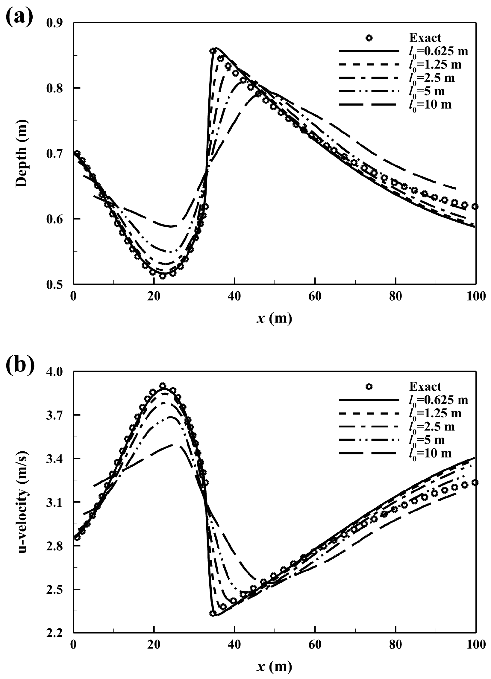
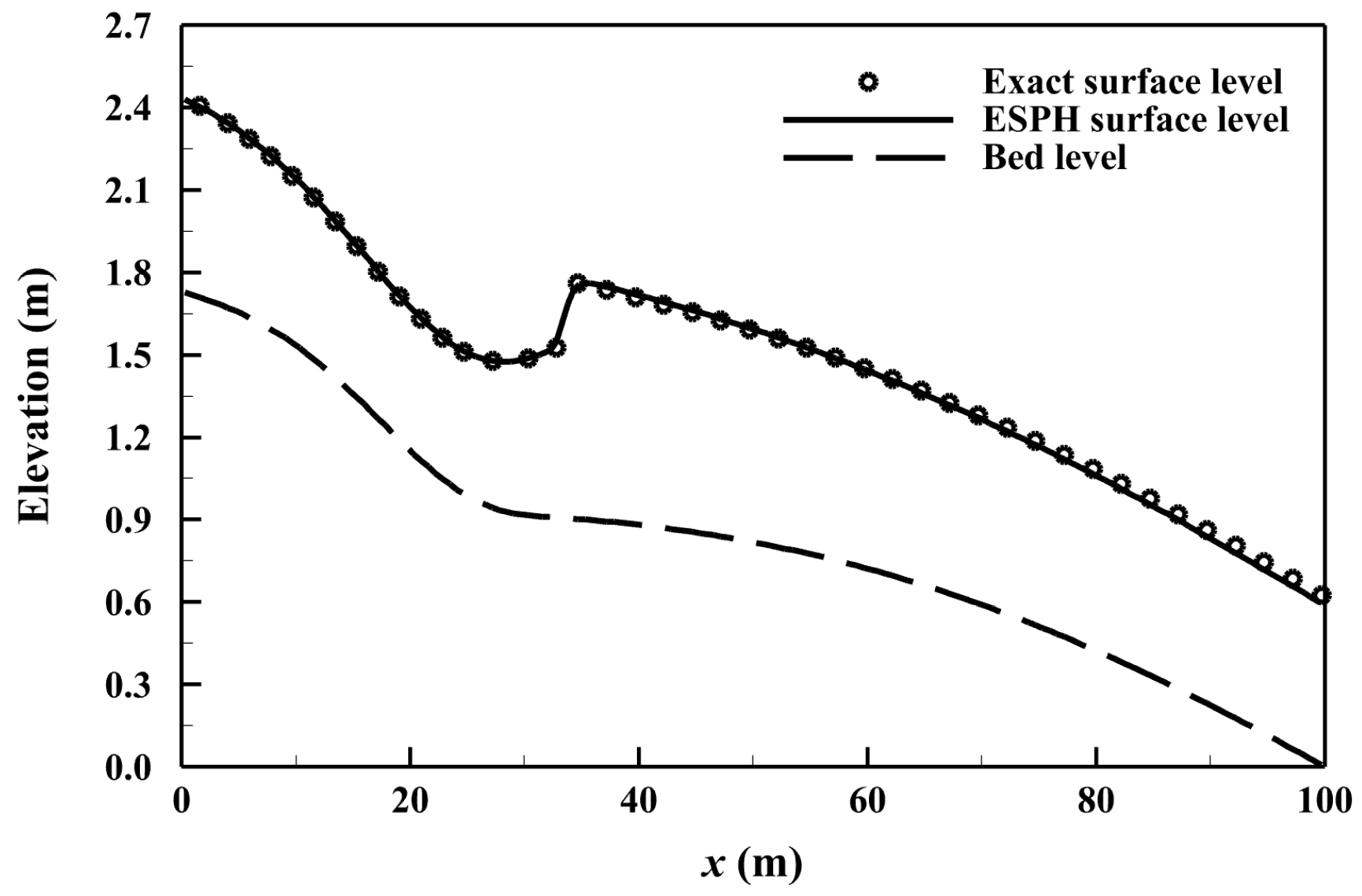
3.1. Analytical Super-Subcritical Flow in a Rectangular Channel

The first case study aims to evaluate the convergence and accuracy of the developed model for open channel flows. An analytical solution for a super-subcritical flow in a rectangular channel, originally solved by MacDonald [42], is selected for this purpose. The channel has a length of 100 m and a width B_w of 80 m, and the bed slope is prescribed by Equation (20). The flow conditions include a discharge Q of 160 m³/s and a Manning’s roughness coefficient n_m of 0.03 s·m^−1/3. Due to the supercritical inflow and outflow conditions, only the inflow discharge (160 m³/s) and inflow water depth (0.706566 m) need to be specified, while no outflow boundary condition is required.

$$S_0(x)=\left(1-{\displaystyle \frac{Q^2}{g{B}_w^{2}h}}\right){\displaystyle \frac{dh}{dx}}+Q^2{n}_m^2{\displaystyle \frac{{\left(2h+B_w\right)}^{\raisebox{1ex}{$4$}\!\left/ \!\raisebox{-1ex}{$3$}\right.}}{{\left(B_{w}h\right)}^{\raisebox{1ex}{$10$}\!\left/ \!\raisebox{-1ex}{$3$}\right.}}}$$

(20)

To evaluate the convergence and accuracy of the developed model, five particle spacings are tested: l₀ = 10 m (100 particles), 5 m (400 particles), 2.5 m (1600 particles), 1.25 m (6400 particles), and 0.625 m (25,600 particles). Figure 1 presents the simulated water depth and u-velocity profiles for each particle spacing. As the resolution increases, the simulated results show improved agreement with the analytical solution, indicating enhanced accuracy at finer particle spacings. The computed convergence rates are 0.7 for water depth and 0.8 for u-velocity, demonstrating that the model achieves approximately first-order convergence. Figure 2 displays the simulated free surface profile at the finest resolution (l₀ = 0.625 m). The bed slope transition at x = 30 m from steep to mild induces a transition from supercritical to subcritical flow, resulting in a hydraulic jump. Downstream of the jump, the water depth gradually increases as the flow returns to supercritical conditions. At the finest resolution, the RRMSEs for water depth and u-velocity are 0.196% and 0.195%, respectively. These results confirm that the developed model can accurately simulate transcritical open channel flows.

3.2. Two-Dimensional Isotropic and Anisotropic Diffusion in Still Water

To evaluate the capability of the developed model in simulating isotropic and anisotropic diffusion, the second case study follows the diffusion scenarios used by Tran-Duc et al. [30], including an isotropic case with D_mx = D_my = 0.10, and two anisotropic cases with D_mx = 0.09 and D_my = 0.03 and D_mx = 0.10 and D_my = 0.01, respectively. The computational domain is a 200 m × 200 m square with a flat and smooth bed. Each simulation is conducted using 160,000 fluid particles, initialized with a water depth of 1 m, zero velocity, and an initial concentration distribution calculated by Equation (21) with t = 0.1 s. Zero-gradient boundary conditions are applied on all four sides. A fixed time step of 0.05 s is used for a total simulation duration of 1800 s.

$$C(x,y,t)={\displaystyle \frac{1}{4\pi t\sqrt{D_{mx}{D}_{my}}}}{{\displaystyle e}}^{-\left({\displaystyle \frac{{\left(x-100\right)}^2}{4D_{mx}t}}+{\displaystyle \frac{{\left(y-100\right)}^2}{4D_{my}t}}\right)}$$

(21)

Figure 3 presents the concentration distributions for the three diffusion scenarios at t = 30 s. The isotropic case (Figure 3a) results in a circular distribution, while the weakly anisotropic case (Figure 3b) produces an elliptical distribution. In contrast, the strongly anisotropic case (Figure 3c) yields a more elongated elliptical distribution, reflecting the greater disparity between D_mx and D_my. Figure 4 compares the simulated and exact concentration profiles along the line y = 100 m for each diffusion scenario. At t = 10 s, the peak concentration in Figure 4c is significantly higher than those in Figure 4a,b. This difference arises from the dominant diffusion in the x-direction in the strongly anisotropic case. Overall, the simulated concentration profiles show good agreement with the exact solutions across all cases. Based on the computed RRMSE values presented in

Table 2. RRMSEs of each diffusion scenario at t = 10 s and 30 s in the second case study.

	Isotropic	Weakly Anisotropic	Strongly Anisotropic
t = 10 s	0.41%	0.26%	0.09%
t = 30 s	0.47%	0.29%	0.10%

, the developed model demonstrates reliable performance in simulating both pure isotropic and anisotropic diffusion processes.

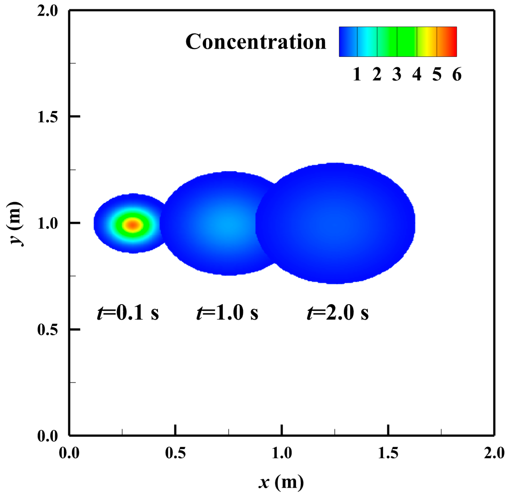
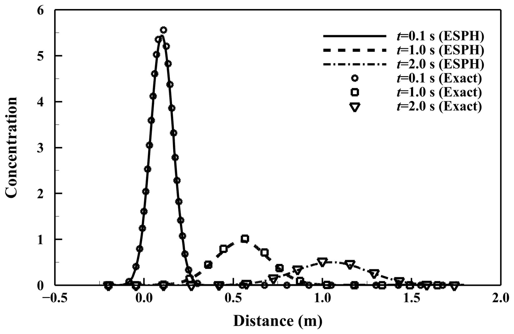
3.3. Advection and Diffusion in a Two-Dimensional Uniform Flow

In the third case study, a 2 m × 2 m square computational domain, previously used by Vanzo et al. [43], is adopted to examine the combined effects of advection and diffusion. A uniform flow with a water depth h = 1 m, velocity u = 0.5 m/s, and velocity v = 0.0 m/s is considered over a flat and smooth bed. The initial concentration distribution is defined according to Equation (22) while D_mx = 0.01 and D_my = 0.005 are given. A particle spacing of 0.005 m (resulting in 160,000 particles) and a fixed time step size of 0.0001 s are used for a total simulation time of 2 s.

$$C(x,y,t)={\displaystyle \frac{0.1}{4\pi th\sqrt{D_{mx}{D}_{my}}}}{{\displaystyle e}}^{-\left[{\displaystyle \frac{{\left(x-ut-0.2\right)}^2}{4D_{mx}t}}+{\displaystyle \frac{{\left(y-vt-0.9975\right)}^2}{4D_{my}t}}\right]}$$

(22)

Figure 5 illustrates the time evolution of the simulated concentration distribution. Due to the diffusion magnitude in the x-direction being twice that in the y-direction, combined with the advection effect of the uniform flow, the initially elliptic distribution becomes further elongated in the x-direction over time and advects downstream with the flow field. Figure 6 presents the comparison between the simulated and exact concentration profiles along the line y = 1 m. From t = 0.1 s to t = 1.0 s, the peak concentration rapidly decays and moves downstream at a constant velocity. The RRMSEs based on concentration at t = 0.1, 1.0, and 2.0 s are 0.16%, 0.29%, and 0.30%, respectively. The close agreement between the simulated and exact results confirms that the developed model is capable of accurately capturing the combined effects of advection and diffusion in open channel flows.

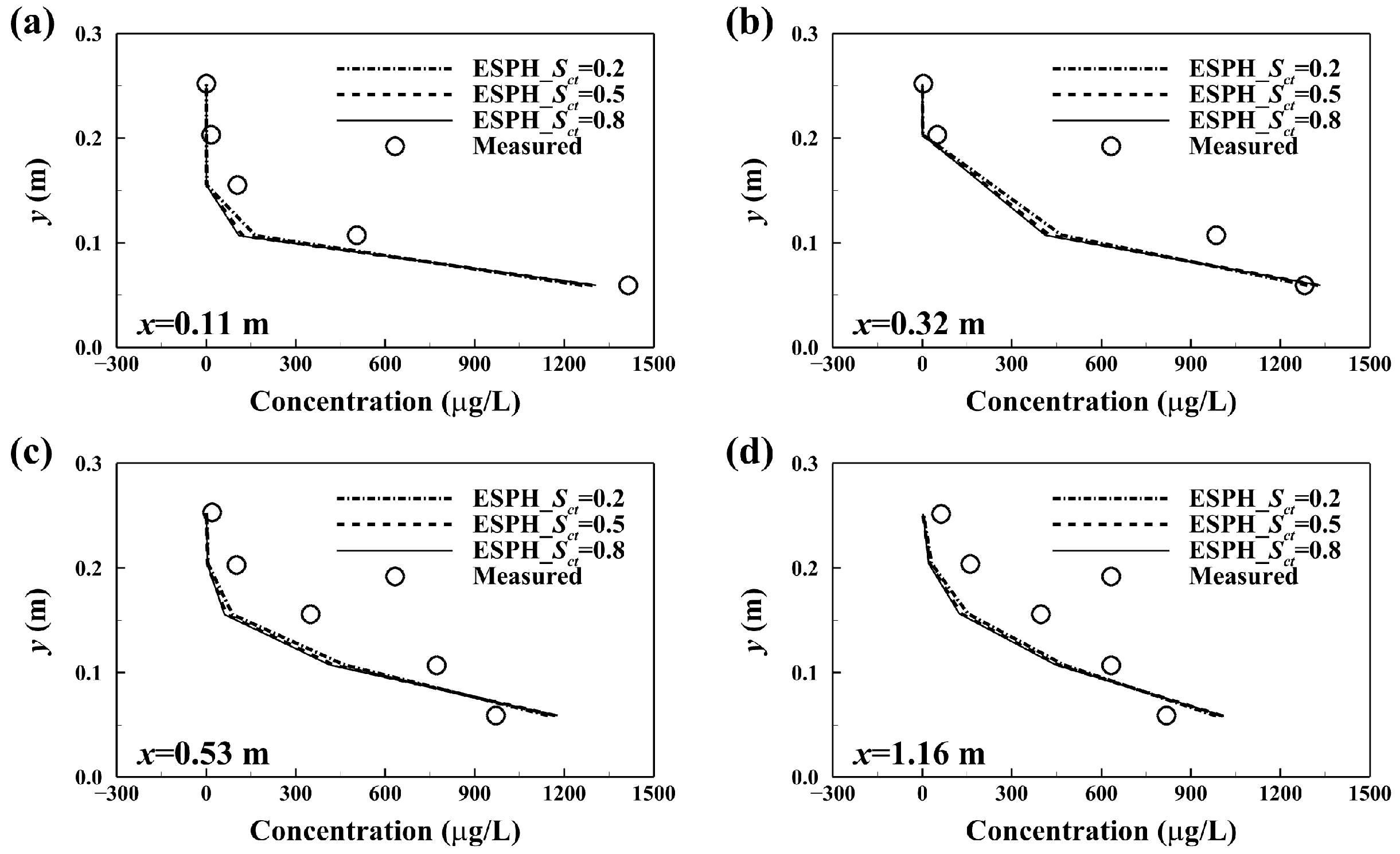
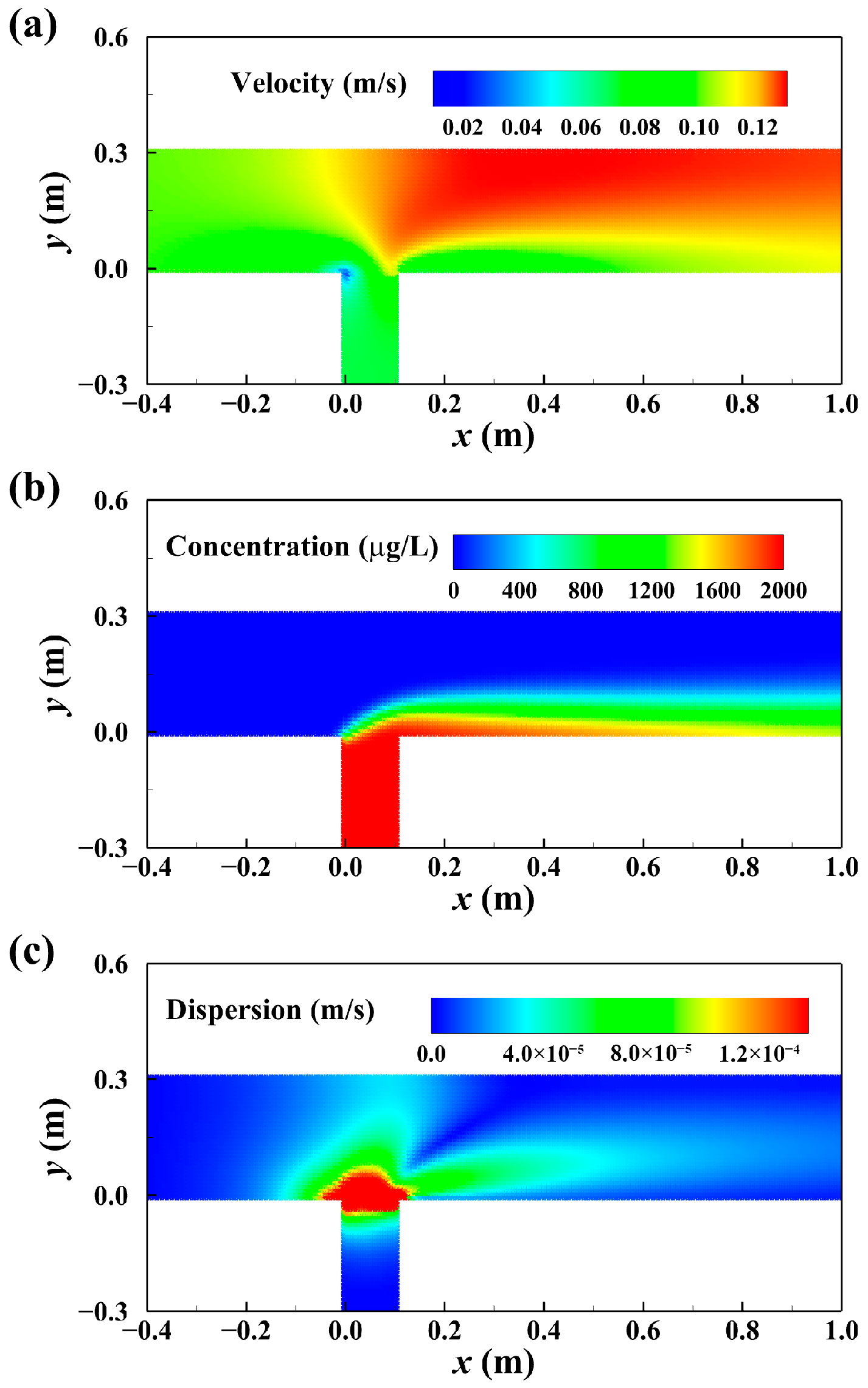
3.4. Two-Dimensional Pollutant Dispersion in a 90° Junction Channel

In the final case study, the developed model is applied to reproduce a laboratory experiment of pollutant dispersion in a 90° junction channel conducted by Chen et al. [44]. Figure 7 illustrates the schematic of the computational domain. The main channel and branch channel are 6.1 m and 1.5 m long, respectively, with widths of 0.3 m and 0.1 m. A discharge of 0.00482 m³/s with zero initial concentration is imposed at the upstream boundary of the main channel, while the water depth at the downstream boundary of the main channel is fixed at 0.16 m. In the branch channel, a discharge of 0.00114 m³/s is prescribed, with a continuously released pollutant concentration of 2000 μg/L. The channel bed is horizontal, and a Manning roughness coefficient of 0.009 s/m^1/3 is assumed. The simulation employs 19,800 fluid particles with a particle spacing l₀ = 0.01 m and a maximum time step of 0.001 s, for a total simulation time of 180 s.

First, sensitivity analysis was conducted using Smagorinsky constants of 0.2 and 0.5. Figure 8 shows the velocity profiles along y = 0.005 m, 0.015 m, and 0.025 m. No significant differences are observed between the two cases. However, as indicated by the RRMSE values in

Table 3. RRMSEs for velocity and concentration in the fourth case study.

	Velocity			Concentration
	Cs			Sct
	0.2	0.5		0.2	0.5	0.8
y = 0.05 m	9.22%	9.14%	x = 0.11 m	11.51%	12.33%	12.58%
y = 0.15 m	1.72%	1.17%	x = 0.32 m	16.04%	17.38%	17.87%
y = 0.25 m	1.58%	1.54%	x = 0.53 m	15.60%	17.23%	17.75%
			x = 1.16 m	14.56%	16.00%	16.40%

, the use of C_s = 0.5 results in slightly improved accuracy. Therefore, C_s = 0.5 is adopted for the remaining simulations. Overall, the simulated velocity profiles agree well with the experimental data, although a slight overestimation is noted at y = 0.005 m. This discrepancy may stem from limitations in the sidewall friction model, which might not fully account for the physical channel wall’s frictional effects.

Next, three turbulent Schmidt numbers—0.2, 0.5, and 0.8—were tested while maintaining C_s = 0.5 to evaluate their influence on the simulated concentration fields. Figure 9 and Table 3 present the concentration profiles and corresponding RRMSE values along x = 0.11 m, 0.32 m, 0.53 m, and 1.16 m. All simulated profiles generally follow the trends observed in the experimental measurements. Among the tested values, S_ct = 0.2 yields the lowest errors. However, across all cases, the simulated concentrations near the center of the cross-section are consistently underestimated compared to the measured values. This suggests a potential underrepresentation of lateral dispersion, likely caused by the simplified treatment of sidewall shear stress in the current model configuration. Despite this limitation, the RRMSE values for both velocity and concentration demonstrate that the developed model provides reliable performance and is well suited for simulating pollutant dispersion in junction channel flows.

Finally, the steady-state distributions of velocity, concentration, and dispersion coefficient (with C_s = 0.5 and S_ct = 0.2) are presented in Figure 10. As the inflow velocity in the main channel is greater than that in the branch channel, the two streams collide at the junction, resulting in the formation of a low-velocity zone near the right wall downstream of the junction (Figure 10a). The concentration distribution shown in Figure 10b indicates that, as the pollutant enters the junction, it disperses along the right downstream wall. This pattern arises because the higher-velocity flow from the main channel suppresses lateral dispersion, confining the pollutant to a narrower region. The dispersion width is approximately 0.1 m. The distribution of the dispersion coefficient, shown in Figure 10c, reveals that dispersion intensity correlates with turbulence magnitude. As expected, the maximum dispersion occurs within the junction region, where the interaction between the two incoming flows generates stronger turbulence.

4. Conclusions

This study presents the development of a new two-dimensional (2D) Eulerian smoothed particle hydrodynamics (ESPH) advection–diffusion model for simulating passive pollutant transport in open channel flows. The model simultaneously solves the 2D shallow water equations and an advection–diffusion equation to capture both hydrodynamic and pollutant concentration fields. To improve numerical stability—particularly in cases involving discontinuities or extremely shallow depths—the model incorporates a hydrostatic reconstruction technique, an HLLC approximate Riemann solver, and an implicit treatment of bed friction. The model’s accuracy and convergence are evaluated through three analytical test cases such as one-dimensional transcritical open channel flow, 2D isotropic and anisotropic diffusion in still water, and advection–diffusion in a 2D uniform flow. The results exhibit first-order convergence and show strong agreement with exact solutions. To further assess its applicability, the model is applied to simulate pollutant transport in a 90° junction channel, reproducing a laboratory experiment. The simulated velocity and concentration profiles generally match the experimental measurements. However, discrepancies are observed near the downstream right-side wall and the center of cross sections, attributed to the simplified treatment of sidewall friction, which may not fully capture the physical wall boundary effects. Specifically, velocity is overestimated near the wall, and concentration is underestimated in the central region. Due to the depth-averaged assumption inherent in the 2D shallow water model, vertical variations in key physical variables—such as velocity and concentration—are not resolved. To capture the full three-dimensional structure of flow and pollutant transport, a fully 3D hydrodynamic model coupled with a Reynolds-averaged turbulence closure and wall function is recommended. Moreover, the uniform particle arrangement adopted in the developed model may restrict its ability to resolve localized flow dynamics in large-scale scenarios, primarily due to computational cost. Future work should focus on incorporating locally refined particle spacing, which would enhance wall boundary representation and improve the model’s accuracy and scalability for real-world environmental applications. Overall, the developed model demonstrates strong potential as a reliable and practical tool for evaluating pollutant transport processes and supporting nature-based solutions in open channels and riverine environments.

References

1. Locke, M.A.; Weaver, M.A.; Zablotowicz, R.M.; Steinriede, R.W.; Bryson, C.T.; Cullum, R.F. Constructed Wetlands as a Component of the Agricultural Landscape: Mitigation of Herbicides in Simulated Runoff from Upland Drainage Areas. Chemosphere 2011, 83, 1532–1538. [Google Scholar] [CrossRef] [PubMed]
2. Winston, R.J.; Hunt, W.F.; Kennedy, S.G.; Merriman, L.S.; Chandler, J.; Brown, D. Evaluation of Floating Treatment Wetlands as Retrofits to Existing Stormwater Retention Ponds. Ecol. Eng. 2013, 54, 254–265. [Google Scholar] [CrossRef]
3. Tournebize, J.; Chaumont, C.; Mander, Ü. Implications for Constructed Wetlands to Mitigate Nitrate and Pesticide Pollution in Agricultural Drained Watersheds. Ecol. Eng. 2017, 103, 415–425. [Google Scholar] [CrossRef]
4. Wu, H.; Wang, R.; Yan, P.; Wu, S.; Chen, Z.; Zhao, Y.; Cheng, C.; Hu, Z.; Zhuang, L.; Guo, Z.; et al. Constructed Wetlands for Pollution Control. Nat. Rev. Earth Environ. 2023, 4, 218–234. [Google Scholar] [CrossRef]
5. Flora, C.; Kröger, R. Use of Vegetated Drainage Ditches and Low-Grade Weirs for Aquaculture Effluent Mitigation: II. Suspended Sediment. Aquac. Eng. 2014, 60, 68–72. [Google Scholar] [CrossRef]
6. Nsenga kumwimba, M.; Zhu, B.; Wang, T.; Dzakpasu, M.; Li, X. Nutrient Dynamics and Retention in a Vegetated Drainage Ditch Receiving Nutrient-Rich Sewage at Low Temperatures. Sci. Total Environ. 2020, 741, 140268. [Google Scholar] [CrossRef] [PubMed]
7. Nsenga kumwimba, M.; Zhu, B.; Moore, M.T.; Wang, T.; Li, X. Can Vegetated Drainage Ditches Be Effective in a Similar Way as Constructed Wetlands? Heavy Metal and Nutrient Standing Stock by Ditch Plant Species. Ecol. Eng. 2021, 166, 106234. [Google Scholar] [CrossRef]
8. Stutter, M.I.; Chardon, W.J.; Kronvang, B. Riparian Buffer Strips as a Multifunctional Management Tool in Agricultural Landscapes: Introduction. J. Environ. Qual. 2012, 41, 297–303. [Google Scholar] [CrossRef] [PubMed]
9. Matos, F.A.; Roebeling, P. Modelling Impacts of Nature-Based Solutions on Surface Water Quality: A Rapid Review. Sustainability 2022, 14, 7381. [Google Scholar] [CrossRef]
10. Liang, Q. A Well-Balanced and Non-Negative Numerical Scheme for Solving the Integrated Shallow Water and Solute Transport Equations. Commun. Comput. Phys. 2010, 7, 1049–1075. [Google Scholar] [CrossRef]
11. Murillo, J.; García-Navarro, P. Improved Riemann Solvers for Complex Transport in Two-Dimensional Unsteady Shallow Flow. J. Comput. Phys. 2011, 230, 7202–7239. [Google Scholar] [CrossRef]
12. Hwang, S.; Son, S. An Efficient HLL-Based Scheme for Capturing Contact-Discontinuity in Scalar Transport by Shallow Water Flow. Commun. Nonlinear Sci. Numer. Simul. 2023, 127, 107531. [Google Scholar] [CrossRef]
13. Zhang, L.; Liang, Q.; Wang, Y.; Yin, J. A Robust Coupled Model for Solute Transport Driven by Severe Flow Conditions. J. Hydro-Environ. Res. 2015, 9, 49–60. [Google Scholar] [CrossRef]
14. Mignot, E.; Riviere, N.; Dewals, B. Formulations and Diffusivity Coefficients of the 2D Depth-Averaged Advection-Diffusion Models: A Literature Review. Water Resour. Res. 2023, 59, e2023WR035053. [Google Scholar] [CrossRef]
15. Ye, T.; Pan, D.; Huang, C.; Liu, M. Smoothed Particle Hydrodynamics (SPH) for Complex Fluid Flows: Recent Developments in Methodology and Applications. Phys. Fluids 2019, 31, 011301. [Google Scholar] [CrossRef]
16. Le Touzé, D.; Colagrossi, A. Smoothed Particle Hydrodynamics for Free-Surface and Multiphase Flows: A Review. Rep. Prog. Phys. 2025, 88, 037001. [Google Scholar] [CrossRef] [PubMed]
17. Chang, K.-H.; Sheu, T.W.-H.; Chang, T.-J. A 1D–2D Coupled SPH-SWE Model Applied to Open Channel Flow Simulations in Complicated Geometries. Adv. Water Resour. 2018, 115, 185–197. [Google Scholar] [CrossRef]
18. Chang, K.-H.; Chang, T.-J.; Garcia, M.H. A Well-Balanced and Positivity-Preserving SPH Method for Shallow Water Flows in Open Channels. J. Hydraul. Res. 2021, 59, 903–916. [Google Scholar] [CrossRef]
19. Vacondio, R.; Rogers, B.D.; Stansby, P.K.; Mignosa, P. SPH Modeling of Shallow Flow with Open Boundaries for Practical Flood Simulation. J. Hydraul. Eng. 2012, 138, 530–541. [Google Scholar] [CrossRef]
20. Chen, R.; Shao, S.; Liu, X.; Zhou, X. Applications of Shallow Water SPH Model in Mountainous Rivers. J. Appl. Fluid Mech. 2015, 8, 863–870. [Google Scholar] [CrossRef]
21. Xia, X.; Liang, Q. A GPU-Accelerated Smoothed Particle Hydrodynamics (SPH) Model for the Shallow Water Equations. Environ. Model. Softw. 2016, 75, 28–43. [Google Scholar] [CrossRef]
22. Tian, L.; Gu, S.; Shao, S.; Wu, Y. Turbulent Models of Shallow-Water Equations-Based Smoothed Particle Hydrodynamics. Phys. Fluids 2024, 36, 107164. [Google Scholar] [CrossRef]
23. Chang, Y.-S.; Chang, T.-J. SPH Simulations of Solute Transport in Flows with Steep Velocity and Concentration Gradients. Water 2017, 9, 132. [Google Scholar] [CrossRef]
24. Liu, W.; Hou, Q.; Lian, J.; Zhang, A.; Dang, J. Coastal Pollutant Transport Modeling Using Smoothed Particle Hydrodynamics with Diffusive Flux. Adv. Water Resour. 2020, 146, 103764. [Google Scholar] [CrossRef]
25. Liu, W.; Hou, Q.; Lei, X.; Lian, J.; Dang, J. SPH Modeling of Substance Transport in Flows with Large Deformation. Front. Environ. Sci. 2022, 10, 991969. [Google Scholar] [CrossRef]
26. Tian, L.; Gu, S.; Wu, Y.; Wu, H.; Zhang, C. Numerical Investigation of Pollutant Transport in a Realistic Terrain with the SPH-SWE Method. Front. Environ. Sci. 2022, 10, 889526. [Google Scholar] [CrossRef]
27. Chang, K.-H. A Novel Eulerian SPH Shallow Water Model for 2D Overland Flow Simulations. J. Hydrol. 2023, 621, 129581. [Google Scholar] [CrossRef]
28. Chang, K.-H.; Wu, Y.-T.; Wang, C.-H.; Chang, T.-J. A New 2D ESPH Bedload Sediment Transport Model for Rapidly Varied Flows over Mobile Beds. J. Hydrol. 2024, 634, 131002. [Google Scholar] [CrossRef]
29. Español, P.; Revenga, M. Smoothed Dissipative Particle Dynamics. Phys. Rev. E 2003, 67, 026705. [Google Scholar] [CrossRef] [PubMed]
30. Tran-Duc, T.; Bertevas, E.; Phan-Thien, N.; Khoo, B.C. Simulation of Anisotropic Diffusion Processes in Fluids with Smoothed Particle Hydrodynamics. Int. J. Numer. Methods Fluids 2016, 82, 730–747. [Google Scholar] [CrossRef]
31. Biriukov, S.; Price, D.J. Stable Anisotropic Heat Conduction in Smoothed Particle Hydrodynamics. Mon. Not. R. Astron. Soc. 2019, 483, 4901–4909. [Google Scholar] [CrossRef]
32. Ru, Z.; Liu, H.; Xing, L.; Ding, Y. A Well-Balanced Lattice Boltzmann Model for the Depth-Averaged Advection–Diffusion Equation with Variable Water Depth. Comput. Methods Appl. Mech. Eng. 2021, 379, 113745. [Google Scholar] [CrossRef]
33. Chaudhry, M.H. Open-Channel Flow; Springer International Publishing: Cham, Switzerland, 2022; ISBN 978-3-030-96446-7. [Google Scholar]
34. Chen, G.; Noelle, S. A New Hydrostatic Reconstruction Scheme Based on Subcell Reconstructions. SIAM J. Numer. Anal. 2017, 55, 758–784. [Google Scholar] [CrossRef]
35. Toro, E.F. Computational Algorithms for Shallow Water Equations; Springer Nature: Cham, Switzerland, 2024; ISBN 978-3-031-61394-4. [Google Scholar]
36. Xia, X.; Liang, Q. A New Efficient Implicit Scheme for Discretising the Stiff Friction Terms in the Shallow Water Equations. Adv. Water Resour. 2018, 117, 87–97. [Google Scholar] [CrossRef]
37. Molls, T.; Zhao, G.; Molls, F. Friction Slope in Depth-Averaged Flow. J. Hydraul. Eng. 1998, 124, 81–85. [Google Scholar] [CrossRef]
38. Morris, J.P.; Fox, P.J.; Zhu, Y. Modeling Low Reynolds Number Incompressible Flows Using SPH. J. Comput. Phys. 1997, 136, 214–226. [Google Scholar] [CrossRef]
39. Smagorinsky, J. General Circulation Experiments with the Primitive Equations: I. The Basic Experiment. Mon. Weather Rev. 1963, 91, 99–164. [Google Scholar] [CrossRef]
40. Van Pham, C.; Deleersnijder, E.; Bousmar, D.; Soares-Frazão, S. Simulation of Flow in Compound Open-Channel Using a Discontinuous Galerkin Finite-Element Method with Smagorinsky Turbulence Closure. J. Hydro-Environ. Res. 2014, 8, 396–409. [Google Scholar] [CrossRef]
41. Gualtieri, C.; Angeloudis, A.; Bombardelli, F.; Jha, S.; Stoesser, T. On the Values for the Turbulent Schmidt Number in Environmental Flows. Fluids 2017, 2, 17. [Google Scholar] [CrossRef]
42. MacDonald, I. Test Problems with Analytic Solutions for Steady Open Channel Flow; Numerical Analysis Reports; University of Reading, Department of Mathematics: Berkshire, UK, 1994. [Google Scholar]
43. Vanzo, D.; Siviglia, A.; Toro, E.F. Pollutant Transport by Shallow Water Equations on Unstructured Meshes: Hyperbolization of the Model and Numerical Solution via a Novel Flux Splitting Scheme. J. Comput. Phys. 2016, 321, 1–20. [Google Scholar] [CrossRef]
44. Chen, K.; Feng, M.; Zhang, T.; Teng, S. Study on distribution of pollutant concentrations in intersection of open channel. J. Hydroelectr. Eng. 2019, 38, 86–100. [Google Scholar] [CrossRef]
Figure 1. Simulated profiles of (a) water depth and (b) u-velocity in the first case study.
Water 17 02205 g001
Figure 2. Simulated free surface profile in the first case study.
Water 17 02205 g002
Figure 3. Simulated concentration distributions at t = 30 s for (a) isotropic, (b) weakly anisotropic, and (c) strongly anisotropic diffusion in the second case study.
Water 17 02205 g003
Figure 4. Simulated concentration profiles along the line y = 100 m for (a) isotropic, (b) weakly anisotropic, and (c) strongly anisotropic diffusion in the second case study.
Water 17 02205 g004
Figure 5. Time evolution of the simulated concentration distribution in the third case study.
Water 17 02205 g005
Figure 6. Simulated concentration profiles at various times along the line y = 1 m in the third case study.
Water 17 02205 g006
Figure 7. Schematic of the computational domain used in the fourth case study.
Water 17 02205 g007
Figure 8. Simulated velocity profiles along y = (a) 0.005 m, (b) 0.015 m, and (c) 0.025 m in the fourth case study.
Water 17 02205 g008
Figure 9. Simulated concentration profiles along x = (a) 0.11 m, (b) 0.32 m, (c) 0.53 m, and (d) 1.16 m in the fourth case study.
Water 17 02205 g009
Figure 10. Steady-state simulated distributions of (a) velocity, (b) concentration, and (c) dispersion coefficient in the fourth case study.
Water 17 02205 g010