Abstract
Accurately monitoring terrestrial water storage (TWS) variations is essential due to global climate change and growing water demands. This study investigates TWS changes in Oregon, USA, using Global Navigation Satellite System (GNSS) data from the Nevada Geodetic Laboratory, Gravity Recovery and Climate Experiment (GRACE) level-3 mascon data from the Jet Propulsion Laboratory (JPL), and Noah model data from the Global Land Data Assimilation System (GLDAS) data. The results show that the GNSS inversion offers superior spatial resolution, clearly capturing a water storage gradient from 300 mm in the Cascades to 20 mm in the basin and accurately distinguishing between mountainous and basin areas. However, the GRACE data exhibit blurred spatial variability, with the equivalent water height amplitude ranging from approximately 100 mm to 145 mm across the study area, making it difficult to resolve terrestrial water storage gradients. Moreover, GLDAS exhibits limitations in mountainous regions. The GNSS can provide continuous dynamic monitoring, with results aligning well with seasonal trends seen in GRACE and GLDAS data, although with a 1–2 months phase lag compared to the precipitation data, reflecting hydrological complexity. Future work may incorporate geological constraints, region-specific elastic models, and regularization strategies to improve monitoring accuracy. This study demonstrates the strong potential of GNSS technology for monitoring TWS dynamics and supporting environmental assessment, disaster warning, and water resource management.
1. Introduction
Terrestrial water storage includes surface water such as rivers and lakes, soil water, groundwater, etc. [1]. Against the backdrop of ongoing global climate warming, frequent occurrences of high temperatures and droughts have led to insufficient supplies of surface water and groundwater [2,3]. Meanwhile, the increasing demand for groundwater resources driven by agricultural and industrial development, as well as population growth, has resulted in the overexploitation of groundwater, further aggravating the water resource crisis [4,5,6]. Therefore, accurately quantifying changes in terrestrial water storage is of great significance for monitoring the health and security of both human and natural ecosystems, and can serve as a basis for local government to formulate water resource management policies [7,8].
The Gravity Recovery and Climate Experiment (GRACE), jointly developed by the United States and Germany, was successfully launched in 2002, thus inaugurating a new era of gravitational field measurement [7]. Since then, the method of estimating terrestrial water storage changes using GRACE gravity satellites has been widely applied in related research worldwide [1,9]. However, a major limitation of GRACE data lies in its spatial resolution of 300–500 km and monthly-scale temporal resolution, which restricts its ability to monitor finer-scale mass changes [10,11]. The follow-up satellite GRACE Follow-On (GFO) led to nearly a year of data gaps during its transition with the GRACE mission, necessitating alternative methods to fill this data void.
The Global Navigation Satellite System (GNSS) plays a critical role in geodetic and geodynamic research [12,13]. Across most regions of the globe, GNSS records primarily reflect the elastic response of the Earth’s crust to surface loads such as snow and precipitation. During autumn and winter, increased surface loading from rainfall and snow causes downward elastic deformation of the crust. During summer, as snow melts and water evaporates, the reduced surface load leads to an upward elastic rebound of the crust [14,15]. Therefore, surface deformation caused by hydrological loading monitored via GNSS can be converted into changes in terrestrial water storage [16,17,18,19].
Recent advances in hydrogeodesy have demonstrated that GNSS-based observations can serve as a powerful complementary tool in conjunction with GRACE/GRACE-FO in resolving terrestrial water storage (TWS) variations, especially at regional scales where GRACE’s coarse resolution is insufficient. Several studies have validated that GNSS vertical displacements, after correcting for non-hydrological signals (e.g., atmospheric, oceanic, thermal effects), can capture seasonal and interannual variations in hydrological loading, offering independent estimates of TWS anomalies [17,18]. For instance, time series decomposition and machine learning techniques such as PCA and VMD-BiLSTM have been applied to GNSS data to extract TWS signals in regions like the Amazon, yielding data in good agreement with that of GRACE, while providing finer spatial detail [20]. Moreover, GNSS-based methods have been successfully applied to quantify groundwater loss in areas like California and the North China Plain [21,22], highlighting their capability for drought monitoring and groundwater management. Sensitivity analyses have shown that the choice of Earth structure models significantly affects TWS estimates from GNSS data—especially at spatial scales <10 km—necessitating careful selection and validation using auxiliary datasets like GRACE [23]. In parallel, GNSS-reflectometry (GNSS-R) has emerged as a valuable approach for retrieving surface parameters like soil moisture, leveraging platforms ranging from ground-based to satellite-borne missions such as CYGNSS, with enhanced accuracy through deep learning integration [24,25]. These developments underscore the growing role of GNSS technologies in water cycle research, enabling higher-resolution and more timely assessments of terrestrial water dynamics.
In areas with a dense distribution of GNSS stations, retrieving water storage changes from GNSS data offers significant advantages, providing monitoring products of terrestrial water storage changes at a higher spatial resolution than that of GRACE [17,18]. Numerous studies have confirmed that GNSS can serve as an independent data source for monitoring terrestrial water storage changes, with related methods achieving significant results [17,18,20,23]. For example, research using GNSS data estimated that groundwater depletion in California’s Central Valley occurred at a rate of 2.2 ± 0.7 km3/year between 2006 and 2021, with a cumulative loss of 45 ± 21 km3 of water during the severe drought period from October 2011 to October 2015 [22].
Given the coarse spatial resolution of GRACE/GFO data, which limits their ability to resolve the spatial distribution of terrestrial water storage in small regions, we focus on using densely distributed GNSS data to estimate the spatial distribution of regional terrestrial water storage changes, analyze their spatial variation characteristics, and compare them with multi-source satellite data.
2. Data Processing and Methods
2.1. GNSS Data and Processing Strategies
The GNSS data used in this study are provided by the Nevada Geodetic Laboratory (NGL), with daily resolution and alignment with the IGS14 frame [12]. The raw data were processed using the GIPSY/OASIS software (Version 6.0) developed by the Jet Propulsion Laboratory (JPL). JPL first determines the orbits of 24 satellites and the positions of 80 ground stations. During processing, corrections were applied for ionospheric delays, tropospheric delays, and antenna phase center deviations. Solid Earth tides, polar tides, and ocean tides were corrected according to the standards of the International Earth Rotation and Reference Systems Service (IERS), but non-tidal loading effects, such as atmospheric, oceanic, and hydrological loading, were not considered [26,27]. To accurately extract surface deformations caused by terrestrial water storage changes, we processed the GNSS data through three steps: (a) using the earthquake occurrence times provided by NGL, the TSAnalyzer tool (v3.2.5.0) was employed to correct step jumps in the GNSS time series caused by antenna replacements or seismic events [28]; (b) a 3σ (three-sigma) method was used to detect and remove gross errors in the time series; (c) environmental loading products released by the German Geoscience Research Center (GFZ) were applied to correct non-tidal atmospheric and oceanic loading displacements in the GNSS observation time series, ensuring that the remaining signals exclusively reflect deformations caused by terrestrial water storage changes.
For each GNSS time series y(t), we model it using the following formula, which includes an intercept term a, a rate term b, and seasonal annual and semi-annual sinusoidal terms, as follows:
where time t is expressed in integer years, and the annual amplitude, Amp, is calculated as
y(t) = a + b · t + Σ (k = 1 to 2) [Cₖ · cos(2πk·t) + Sₖ · sin(2πk·t)]
Amp = sqrt (C12 + S12)
2.2. GRACE Data
In this study, the GRACE data product used is the JPL level-3 mascon (mass concentration) product, which divides the Earth into numerous discrete blocks and assumes uniform mass distribution within each block. The mass change of each block is expressed in equivalent water height. This product has been corrected for glacial isostatic adjustment (GIA), non-tidal atmospheric and oceanic effects, ocean tides, and high-frequency solid tide signals [29], with low-degree terms replaced [30,31,32], and it can be used directly. Compared with traditional spherical harmonic solutions, the mascon product is less affected by gravitational signal leakage outside specific regions and applies spatial and temporal regularization constraints to reduce correlated errors (i.e., north–south striping artifacts) [26].
2.3. Hydrological Model Data
The changes in terrestrial water storage can also be quantitatively estimated using hydrological models. This study uses the Noah hydrological model, released by the Global Land Data Assimilation System (GLDAS). The model integrates both ground-based and satellite observational data products, including components such as surface water, soil moisture, canopy water, and snow water equivalent. It generates optimal fields of surface states and fluxes through advanced techniques in surface modeling and data assimilation. The GLDAS hydrological model can not only be used to study the evolution of terrestrial hydrological loading but can also be applied in climate simulation, meteorological forecasting, and assessing water resource sustainability. The GLDAS monthly surface hydrological model used here has a spatial resolution of 0.25° × 0.25°. Data for the GLDAS shallow surface hydrological model can be downloaded at https://disc.gsfc.nasa.gov/datasets?keywords=GLDAS (accessed on 20 May 2025).
2.4. TRMM_3B43 Rainfall Data
Terrestrial water storage is closely related to precipitation, and we also collected TRMM_3B43 rainfall data for empirical validation. The TRMM (Tropical Rainfall Measuring Mission) rainfall data are global precipitation datasets obtained from a joint satellite remote sensing mission conducted by NASA (National Aeronautics and Space Administration) and JAXA (Japan Aerospace Exploration Agency). Launched in 1997, the primary objective of the TRMM satellite mission was to observe precipitation in tropical regions and provide critical data for studying global precipitation patterns and monitoring climate change. The TRMM_3B43 rainfall data are collected by instruments such as the satellite’s microwave imager (TMI) and radar system (PR), covering regions near the equator (approximately ±50° latitude). The satellite scans the Earth’s surface every few hours to generate precipitation data. This data product is released in a gridded format, with a spatial resolution of 0.25° × 0.25° and a monthly temporal resolution spanning from 1998 to 2019, capable of providing large-scale, long-term precipitation information.
2.5. Method for Inverting Terrestrial Water Storage by GNSS
There is a relatively high density distribution of GNSS stations in the state of Oregon, allowing us to invert mass changes with higher spatial resolution. The study area (latitude: 41.5°–46.5° N, longitude: 125°–116° W) is subdivided into 0.25° × 0.25° grids. Using the vertical displacements from all GNSS stations within the study area as observations, the well-known Green’s function is used to relate surface displacements to changes in surface mass [33]. For point load, the resulting vertical displacement observed by GNSS can be expressed as
where u is the vertical displacement (m), m is the load mass (kg), G is the Green’s function related to the angular distance between the point load and the GNSS station, and δ_error is the observation error. Typically, we define an objective function for minimizing errors to solve the problem, which is expressed as
u = G · m + δ_error
min {||G · m − u||2}
However, since the number of unknown parameters for mass changes far exceeds the number of GNSS observations, the Green’s function coefficient matrix G is rank-deficient and cannot be directly solved. Therefore, additional constraints are required to invert the mass change parameters. Here, the Laplace operator L is used as an additional constraint to smooth the solution, and the Tikhonov regularization method is employed for solving. The objective function then becomes
after considering the Laplace constraint, the solution for mass, m, is
where P is the weight matrix of GNSS observations, and u and k are unknown non-negative parameters representing the roughness factor, which quantifies the difference between adjacent pixel values. There are multiple methods to determine k, including principal component estimation [34], Bayesian information criterion, and the L-curve method [35]. Here, we use generalized cross validation (GCV) [36] to determine the roughness factor, which operates by solving for the variable that minimizes the GCV function. The Laplace operator L has a template form, as follows:
However, the L1 cannot smooth the edges effectively. To solve this problem, this paper introduces two templates, namely, the L2 template and the L3 template:
min {||G · m − u||2 + k2·||L(m)||2}
m = (Gᵗ · P · G + k · Lᵗ·L)−1 · Gᵗ · P · u
L1 = [ [0, 1, 0], [1, −4, 1], [0, 1, 0] ]
L2 = [1; −2; 1], L3 = [1, −2, 1]
3. Results and Analysis of Land Water Storage Inversion by GNSS
Using the GNSS vertical position time series, we inverted three types of terrestrial water storage changes in Oregon: (1) checkerboard test simulations, (2) terrestrial water storage changes over time, and (3) the spatial distribution of multi-year average seasonal terrestrial water storage.
3.1. Simulation Test
Since the inversion of terrestrial water storage using GNSS is influenced by the locations of the GNSS stations, we conducted a checkerboard test to verify the sensitivity and robustness of our inversion method. Figure 1 show the input model and inversion results of the checkerboard test, respectively, to evaluate the spatial resolution and robustness of the inversion method. Figure 1a shows the synthetic input model (alternating positive and negative TWS anomalies), and Figure 1b shows the inversion results based on simulated GNSS station distribution. The test demonstrates that with the dense distribution of GNSS stations in Oregon, the input model for the region can be well recovered, confirming the sensitivity of the method. However, due to the constraints of the Laplace operator, the inversion results are smoother than those of the true input model.
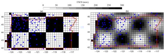
Figure 1.
Checkerboard test in Oregon: (a) synthetic input model (alternating positive and negative TWS anomalies); (b) inversion results based on simulated GNSS station distribution. The red line represents the boundary of the study region.
3.2. Land Water Storage Changes over Time
To investigate terrestrial water storage changes at higher temporal resolutions, we used detrended GNSS vertical time series to invert the spatiotemporal water load changes in Oregon. Terrestrial water storage changes in Oregon from 2015 to 2020 were calculated using Equation (4). With the aid of the high temporal resolution of GNSS, we obtained daily terrestrial water storage changes (Figure 2). The long-term trend reveals strong interannual periodic variations in Oregon. We also show the time-varying regional average equivalent water height (EWH) time series derived using two independent techniques: GRACE and the GLDAS hydrological model. These three EWH time series exhibit good consistency. Additionally, we present the average precipitation change curve for the state, clearly demonstrating a strong correlation between the three terrestrial water storage solutions and precipitation. The TWS typically reaches its maximum, around 150 mm equivalent water height, between January and April each year, and its minimum, around −150 mm equivalent water height, between July and October.
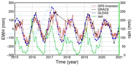
Figure 2.
Changes in terrestrial water storage.
To further investigate the spatiotemporal patterns of terrestrial water storage (TWS) in the region, we also present maps of monthly mean TWS distributions. As shown in Figure 3, Figure 4, Figure 5, Figure 6, Figure 7 and Figure 8, TWS in Oregon reaches its annual minimum during summer, with values as low as −300 mm equivalent water height. This is primarily due to high temperatures causing snowmelt and soil moisture evaporation. In winter, TWS reaches its annual maximum of up to a 300 mm equivalent water height, driven by rainfall and snowfall, which aligns with the known hydrological conditions of the region. Moreover, both GRACE and GLDAS data show that the TWS variations inverted from GNSS are in good agreement with observational and model values. This indicates that the inversion accuracy meets the requirements for TWS monitoring in the region, and that GNSS vertical displacements effectively capture the elastic response of the solid Earth to seasonal terrestrial water variations.
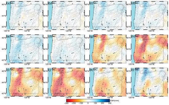
Figure 3.
Monthly spatial and temporal terrestrial water storage changes in Oregon for the year 2015. (a) January; (b) February; (c) March; (d) April; (e) May; (f) June; (g) July; (h) August; (i) September; (j) October; (k) November; (l) December.
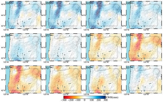
Figure 4.
Monthly spatial and temporal terrestrial water storage changes in Oregon for the year 2016. (a) January; (b) February; (c) March; (d) April; (e) May; (f) June; (g) July; (h) August; (i) September; (j) October; (k) November; (l) December.
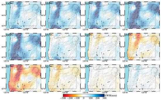
Figure 5.
Monthly spatial and temporal terrestrial water storage changes in Oregon for the year 2017. (a) January; (b) February; (c) March; (d) April; (e) May; (f) June; (g) July; (h) August; (i) September; (j) October; (k) November; (l) December.
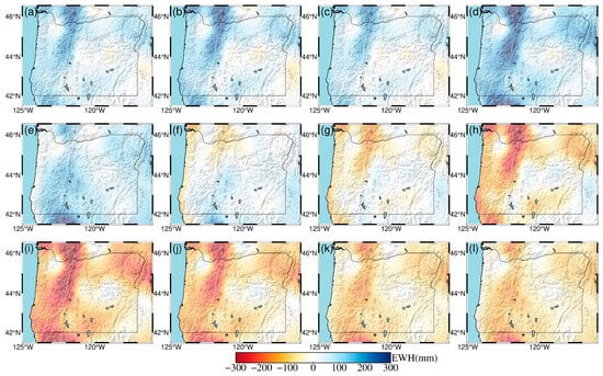
Figure 6.
Monthly spatial and temporal terrestrial water storage changes in Oregon for the year 2018. (a) January; (b) February; (c) March; (d) April; (e) May; (f) June; (g) July; (h) August; (i) September; (j) October; (k) November; (l) December.
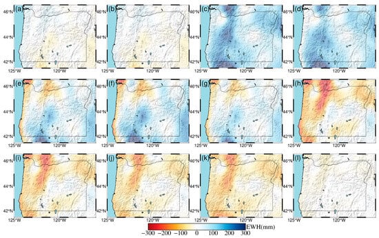
Figure 7.
Monthly spatial and temporal terrestrial water storage changes in Oregon for the year 2019. (a) January; (b) February; (c) March; (d) April; (e) May; (f) June; (g) July; (h) August; (i) September; (j) October; (k) November; (l) December.
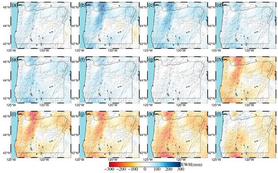
Figure 8.
Monthly spatial and temporal terrestrial water storage changes in Oregon for the year 2020. (a) January; (b) February; (c) March; (d) April; (e) May; (f) June; (g) July; (h) August; (i) September; (j) October; (k) November; (l) December.
3.3. Spatial Distribution of Seasonal Terrestrial Water Storage Amplitude
To investigate the spatial distribution of terrestrial water storage, we present the annual amplitude of terrestrial water storage inverted using three independent techniques—GNSS, GRACE, and GLDAS—for Oregon, as shown in Figure 9a–c. The annual amplitude at each grid point is derived by fitting the time series using Equations (1) and (2), which extract the seasonal (annual) harmonic component. Figure 9a reveals that the annual mean equivalent water height (EWH) amplitude of terrestrial water storage (TWS) estimated by GNSS in Oregon reaches up to 300 mm, with the maximum observed in the Cascade Mountains near the northern border with Washington State. The amplitude gradually decreases from the mountains toward the adjacent basins, ranging from 20 to 100 mm, and also diminishes from north to south along the mountain range. Figure 9b illustrates the spatial distribution of long-term average seasonal TWS variations derived from GRACE data. Due to GRACE’s coarse spatial resolution (~300 km), the spatial variation across the study area is not obvious, and the amplitude is minimal. The amplitude in the southern part is approximately 100 mm, slightly lower than the 145 mm observed in the north, with a difference of less than 50 mm. Furthermore, the annual amplitude in the Cascade Mountains is about 150 mm, which is significantly smaller than the 300 mm annual TWS amplitude derived from the GNSS inversion. Figure 9c shows the spatial distribution of terrestrial water storage from the GLDAS hydrological model, which is primarily divided into the eastern and western parts. The average amplitude in the western region is approximately 250 mm, which is greater than the 50–100 mm observed in the eastern region. This is consistent with the GNSS results, as the Cascade Range in the east exhibits pronounced seasonal variations. However, west of the mountains, GLDAS’s spatial features are coarser compared to those of GNSS, and the maximum amplitude of seasonal changes calculated by the GLDAS hydrological model is 250 mm, which is less than that of the annual amplitude, about 300 mm, inverted by GNSS. Collectively, these results demonstrate that GNSS can resolve the spatial distribution of terrestrial water storage in this region with higher spatial resolution.
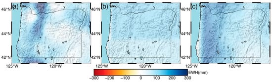
Figure 9.
Spatial distribution of seasonal amplitude of terrestrial water storage changes inferred by (a) GNSS; (b) GRACE; (c) GLDAS.
4. Discussion
This study investigates terrestrial water storage (TWS) changes in Oregon, USA, by inverting GNSS vertical position time series data and performing a comparative analysis using GRACE satellite data and the GLDAS hydrological model. The study explores in depth the coupling mechanisms between the surface hydrological system and the elastic response of the crust, summarizes key findings and limitations, and provides guidance for future research.
The checkerboard test shows that the GNSS-inverted TWS results are smoother than those of the true input model, mainly due to the influence of relatively dense GNSS station distribution and the constraints imposed by the Laplacian operator.
When examining the spatial annual amplitude variations in TWS derived from GNSS vertical deformation, the GNSS results display clear gradient features, consistent with the accumulation and release patterns of TWS driven by precipitation and snowmelt in mountainous regions. In contrast, GRACE shows little spatial variability, while GLDAS, although capable of indicating gradient changes, exhibits coarse spatial characteristics in regions with weak seasonal variations. This can be attributed to GRACE’s relatively coarse spatial resolution and potential gravity field errors, which limit its ability to provide accurate and detailed data for regional hydrological processes or fine-scale TWS changes. Additionally, GRACE data exhibits data discontinuities, such as the data void between 2017 and 2018 following the end of the GRACE mission and before GRACE-FO became operational.
GLDAS standard products typically display spatial resolutions of 0.25° to 1° (approximately 25–100 km), making it challenging to capture hydrological process details in regions with complex terrain (e.g., mountains, small catchments) or high land-use heterogeneity (e.g., urban areas, farmlands). For example, local precipitation, soil moisture, and runoff in mountainous regions may show significant spatial variability due to topographic differences, but coarse-resolution models tend to average out these differences, leading to simulation errors. Furthermore, the model simulates multilayer soil moisture (e.g., 0–10 cm, 10–40 cm), which may present vertical scale mismatch issues during direct assimilation.
Although GNSS excels in high-resolution monitoring, its inversion accuracy is highly dependent on station density and data quality. In areas with sparse stations or near the boundaries of the study area, inversion performance can deteriorate significantly due to insufficient observations. Moreover, most mainstream crustal elastic models are based on the assumption of a homogeneous elastic half-space and fail to adequately account for local geological heterogeneity, lithological contrasts, or complex 3D crustal structures. Therefore, such simplifications may introduce systematic errors into the inversion results.
In terms of regional time series inversion, although the GNSS-derived TWS results exhibit strong agreement with GRACE and GLDAS data, they show a 1–2 month phase lag compared with the data for precipitation series. This phenomenon highlights the buffering and regulating properties of the hydrological system, indicating that TWS changes are not solely driven by precipitation but are also modulated by multiple hydrological processes such as evapotranspiration, soil infiltration, and groundwater recharge. This finding not only reflects the complexity of hydrological processes but also suggests higher requirements for parameter optimization and process simulation in current hydrological models.
Based on the above discussion, future research could be further advanced in the following aspects: (1) introducing geological structural constraints or regionally varying elastic models to enhance the physical realism of crustal response modeling; (2) developing regularization strategies adapted to station spatial distribution characteristics to improve inversion stability and boundary fidelity in sparse station regions. These efforts would further improve the spatiotemporal accuracy and interpretability of TWS monitoring and help fill the observational gaps between the GRACE and GFO missions.
5. Conclusions
This study employed GNSS data to invert terrestrial water storage (TWS) changes in Oregon, USA, with the following key conclusions:
- (1)
- The TWS in Oregon exhibits obvious interannual periodic variations. The equivalent water height (EWH) reaches peak values between January and April each year (maximum of approximately 150 mm), while troughs occur between July and October (minimum of approximately −150 mm), showing strong consistency with regional precipitation cycles. During summer (June–August), high temperatures lead to snowmelt and soil moisture evaporation, causing TWS to reach its annual minimum, with EWH in the Cascade Mountains dropping to as low as −300 mm. In winter (December–February), rainfall and snowfall increase TWS to peak levels (up to 300 mm), with spatial patterns consistent with the region’s climate and topographic features.
- (2)
- The daily-scale dynamic variations in TWS inverted from GNSS data show good agreement with GRACE satellite observations and GLDAS hydrological model results, confirming the reliability of the inversion. The multi-year average seasonal amplitude indicates that GNSS-inverted EWH amplitude reaches a maximum of 300 mm in the northern Cascade Mountains, decreasing toward surrounding basins.
- (3)
- Compared with traditional methods, the GNSS inversion approach offers distinct advantages in regards to both spatial and temporal resolution. With the aid of a dense GNSS station distribution, it enables the resolution of fine-scale local variations that are difficult to capture using conventional methods (e.g., amplitude differences across mountain slopes). The spatial details of the inversion results (such as the 300 mm amplitude peak) are significantly superior to those of GRACE (spatial resolution ≈300 km, capturing only regional averages), while the daily monitoring capability of the time series greatly outperforms the monthly resolution of GRACE and the limited dynamic response of the GLDAS model.
Author Contributions
Conceptualization, H.C. and J.Q.; methodology, J.Q.; software, D.W.; validation, D.W., J.Q., and H.C.; formal analysis, D.W.; investigation, D.W.; resources, J.Q.; data curation, D.W.; writing—original draft preparation, D.W.; writing—review and editing, H.C. and J.Q.; visualization, D.W.; supervision, J.Q.; project administration, H.C.; funding acquisition, J.Q. All authors have read and agreed to the published version of the manuscript.
Funding
This research received no external funding.
Data Availability Statement
Data used during the study will be made available upon reasonable request to the corresponding author.
Acknowledgments
The authors would like to gratefully acknowledge that the study presented in this paper is supported by Guangzhou Salvage in China, Nanyang Technological University in Singapore, and the Tianjin Research Institute for Water Transport Engineering Co., Ltd., in China.
Conflicts of Interest
Author Jian Qin was employed by Tianjin Water Transport Engineering Research Institute Co., Ltd. Author Dejian Wu was employed by Guangzhou Salvage, Guangzhou. The remaining authors declare that the research was conducted in the absence of any commercial or financial relationships that could be construed as a potential conflict of interest.
Abbreviations
The following abbreviations are used in this manuscript:
| GRACE | Gravity Recovery and Climate Experiment |
| GLDAS | Global Land Data Assimilation System |
| GNSS | Global Navigation Satellite System |
| NGL | Nevada Geodetic Laboratory |
| JPL | Jet Propulsion Laboratory |
| TWS | Terrestrial Water Storage |
| EWH | Equivalent Water Height |
References
- Rodell, M.; Velicogna, I.; Famiglietti, J.S. Satellite-based estimates of groundwater depletion in India. Nature 2009, 460, 999–1002. [Google Scholar] [CrossRef] [PubMed]
- Famiglietti, J.S. The global groundwater crisis. Nat. Clim. Change 2014, 4, 945–948. [Google Scholar] [CrossRef]
- Trenberth, K.E.; Dai, A.; Van Der Schrier, G.; Jones, P.D.; Barichivich, J.; Briffa, K.R.; Sheffield, J. Global warming and changes in drought. Nat. Clim. Change 2014, 4, 17–22. [Google Scholar] [CrossRef]
- Wada, Y.; Van Beek, L.P.H.; Van Kempen, C.M.; Reckman, J.W.T.M.; Vasak, S.; Bierkens, M.F.P. Global depletion of groundwater resources. Geophys. Res. Lett. 2010, 37, L20402. [Google Scholar] [CrossRef]
- Konikow, L.F. Contribution of global groundwater depletion since 1900 to sea-level rise. Geophys. Res. Lett. 2011, 38. [Google Scholar] [CrossRef]
- Scanlon, B.R.; Faunt, C.C.; Longuevergne, L.; Reedy, R.C.; Alley, W.M.; McGuire, V.L.; McMahon, P.B. Groundwater depletion and sustainability of irrigation in the US High Plains and Central Valley. Proc. Natl. Acad. Sci. USA 2012, 109, 9320–9325. [Google Scholar] [CrossRef] [PubMed]
- Tapley, B.D.; Bettadpur, S.; Ries, J.C.; Thompson, P.F.; Watkins, M.M. GRACE measurements of mass variability in the Earth system. Science 2004, 305, 503–505. [Google Scholar] [CrossRef] [PubMed]
- Long, D.; Longuevergne, L.; Scanlon, B.R. Deriving groundwater storage changes in China from GRACE with an improved approach. Remote Sens. Environ. 2013, 129, 79–91. [Google Scholar]
- Wahr, J.; Molenaar, M.; Bryan, F. Time variability of the Earth’s gravity field. JGR Solid Earth 1998, 103, 30205–30229. [Google Scholar]
- Long, D.; Chen, X.; Scanlon, B.R.; Wada, Y.; Hong, Y.; Singh, V.P.; Chen, Y.; Wang, C.; Han, Z. Have GRACE satellites overestimated groundwater depletion in the Northwest India Aquifer? Sci. Rep. 2015, 5, 12843. [Google Scholar] [CrossRef] [PubMed]
- Razeghi, M.; Han, S.-C.; McClusky, S.; Sauber, J. A Joint Analysis of GPS Displacement and GRACE Geopotential Data for Simultaneous Estimation of Geocenter Motion and Gravitational Field. J. Geophys. Res. Solid Earth 2019, 124, 11. [Google Scholar] [CrossRef]
- Blewitt, G.; Hammond, W.; Kreemer, C. Harnessing the GPS data explosion for science. Eos 2018, 99, e2020943118. [Google Scholar] [CrossRef]
- Calais, E.; Dong, L.; Wang, M.; Shen, Z.; Vergnolle, M. Continental deformation in Asia from a combined GPS solution. Geophys. Res. Lett. 2006, 33, L08303. [Google Scholar] [CrossRef]
- Van Dam, T.; Wahr, J.; Milly, P.C.D.; Shmakin, A.B.; Blewitt, G.; Lavallée, D.; Larson, K.M. Crustal displacements due to continental water loading. Geophys. Res. Lett. 2001, 28, 651–654. [Google Scholar] [CrossRef]
- Tregoning, P.; Watson, C.; Ramillien, G. Effects of snow and ice mass variations on seasonal deformation in the western Himalaya. GRL 2009, 36. [Google Scholar] [CrossRef]
- Argus, D.F.; Landerer, F.W.; Wiese, D.N.; Martens, H.R.; Fu, Y.; Famiglietti, J.S.; Thomas, B.F.; Farr, T.G.; Moore, A.W.; Watkins, M.M. Sustained water loss in California’s mountain ranges. JGR Solid Earth 2017, 44, 6247–6255. [Google Scholar]
- Fu, Y.; Chen, Y.W.; Hsu, Y.J.; Shum, C.K.; Chiang, H.W. Inversion of terrestrial water storage from GNSS in Taiwan. JGR Solid Earth 2021, 126, e2020JB021157. [Google Scholar]
- Jiang, Y.; Li, X.; Zhang, H.; Wang, J. Terrestrial water storage from GNSS vertical displacement: Sichuan case. Water 2021, 13, 961. [Google Scholar]
- Swarr, M.A.; Moore, A.W.; Lavallée, D.; Blewitt, G. Sensitivity of GNSS-Derived Estimates of Terrestrial Water Storage to Assumed Earth Structure. JGR Solid Earth. 2024, 129. [Google Scholar] [CrossRef]
- Liu, Y.; Xu, K.; Guo, Z.; Li, S.; Zhu, Y. GNSS and GRACE fusion using PCA and VMD-BiLSTM. Sci. Total Environ. 2021, 776, 145758. [Google Scholar]
- Tangdamrongsub, N.; Blewitt, G.; Liang, C.; Shen, Z. High-resolution TWS from GPS and GRACE in North China Plain. JGR Solid Earth 2017, 122, 6940–6959. [Google Scholar]
- Li, J.; Zhang, X.; Wang, C.; Shen, Z. Monitoring drought-induced groundwater loss using GPS. JGR Solid Earth 2021, 126, e2021JB022489. [Google Scholar]
- Jiang, Z.; Hsu, Y.J.; Yuan, L.; Feng, W.; Yang, X.; Tang, M. GNSS-derived TWS error sensitivity. ETH Res. Collect. 2022, 26, 1–7. [Google Scholar]
- Alemohammad, S.H.; Madani, K.; Zhao, X.; Zadeh, M.S.; Kaymakci, E.; Mahmoodian, S. Review of GNSS-R soil moisture retrieval. Remote Sens. 2021, 13, 1350. [Google Scholar]
- Wang, W.; Li, X.; Zhang, Y.; Chen, Z.; Liu, H.; Zhao, S. GNSS-R and meteorological fusion for soil moisture. Environ. Syst. Res. 2024, 13, 2. [Google Scholar]
- Carlson, G.; Werth, S.; Shirzaei, M. Joint Inversion of GNSS and GRACE for Terrestrial Water Storage Change in California. J. Geophys. Res. Solid Earth 2022, 127, e2021JB023135. [Google Scholar] [CrossRef] [PubMed]
- Blewitt, G.; Kreemer, C.; Hammond, W.C.; Goldfarb, J.M. Terrestrial reference frame NA12 for crustal deformation studies in North America. J. Geodyn. 2013, 72, 11–24. [Google Scholar] [CrossRef]
- Wu, D.; Yan, H.; Shen, Y. TSAnalyzer, A GNSS time series analysis software. GPS Solut. 2017, 21, 1389–1394. [Google Scholar] [CrossRef]
- Peltier, W.R.; Argus, D.; Drummond, R. Space geodesy constrains ice age terminal deglaciation: The global ICE-6G_C (VM5a) model. J. Geophys. Res. Solid Earth 2015, 120, 450–487. [Google Scholar] [CrossRef]
- Sun, Y.; Riva, R.; Ditmar, P. Optimizing estimates of annual variations and trends in geocenter motion and J2 from a combination of GRACE data and geophysical models. J. Geophys. Res. Solid Earth 2016, 121, 8352–8370. [Google Scholar] [CrossRef]
- Swenson, S.; Chambers, D.; Wahr, J. Estimating geocenter variations from a combination of GRACE and ocean model output. J. Geophys. Res. Solid Earth 2008, 113, JB005338. [Google Scholar] [CrossRef]
- Loomis, B.D.; Rachlin, K.E.; Wiese, D.N.; Landerer, F.W.; Luthcke, S.B. Replacing GRACE/GRACE-FO with satellite laser ranging: Impacts on Antarctic Ice Sheet mass change. Geophys. Res. Lett. 2020, 47, e2019GL085488. [Google Scholar] [CrossRef]
- Farrell, W. Deformation of the Earth by surface loads. Rev. Geophys. 1972, 10, 761–797. [Google Scholar] [CrossRef]
- Xu, P.L.; Rummel, R. A Simulation Study of Smoothness Methods in Recovery of Regional Gravity Fields. Geophys. J. Int. 1994, 117, 472–486. [Google Scholar] [CrossRef]
- Hansen, P.C. Analysis of Discrete Ill-Posed Problems by Means of the L-Curve. Siam Rev. 1992, 34, 561–580. [Google Scholar] [CrossRef]
- Golub, G.H.; Heath, M.; Wahba, G. Generalized cross-validation as a method for choosing a good ridge parameter. Technometrics 1979, 21, 215–223. [Google Scholar] [CrossRef]
Disclaimer/Publisher’s Note: The statements, opinions and data contained in all publications are solely those of the individual author(s) and contributor(s) and not of MDPI and/or the editor(s). MDPI and/or the editor(s) disclaim responsibility for any injury to people or property resulting from any ideas, methods, instructions or products referred to in the content. |
© 2025 by the authors. Licensee MDPI, Basel, Switzerland. This article is an open access article distributed under the terms and conditions of the Creative Commons Attribution (CC BY) license (https://creativecommons.org/licenses/by/4.0/).