Abstract
Coastal areas are increasingly vulnerable to erosion, a process that can lead to severe consequences such as flooding and land loss. This study investigates strategies for preventing and mitigating coastal erosion, with a particular focus on nature-based solutions, notably artificial sand nourishment. Artificial nourishment has proven to be an effective method for erosion control. However, its success depends on factors such as the placement location, sediment volume, and frequency of operations. To optimize these interventions, simulations were conducted using both a numerical model (CS-Model) and a physical flume model, based on the same cross-section beach/dune profile, to compare cross-shore nourishment performance across different scenarios. The numerical modeling approach is presented first, including a description of the reference prototype-scale scenario. This is followed by an overview of the physical modeling, detailing the experimental 2D cross-section flume setup and tested scenarios. These scenarios simulate nourishment interventions with variations in beach profile, aiming to assess the influence of water level, berm width, bar volume, and bar geometry. The results from both numerical and physical simulations are presented, focusing on the cross-shore morphological response of the beach profile under wave action, particularly the effects on profile shape, water level, bar volume, and the position and depth of the bar crest. The main conclusion highlights that a wider initial berm leads to greater wave energy dissipation, thereby contributing to the mitigation of dune erosion.
1. Introduction
Sandbar–beach–dune systems are highly dynamic features exposed to waves and currents, particularly during extreme events. Their evolution is mainly governed by the complex exchange of sediments through hydrodynamic processes. In particular, during storms and surges, the action of waves can cause severe erosion, with widespread morphological changes, namely in the bar volumes, beach berm width, and/or slope. In fact, coastal erosion poses a significant threat to sandy shorelines worldwide, driven by a complex combination of natural and anthropogenic factors. Key processes include wave action, storm surges, sea-level rise, and sediment transport dynamics, all of which interact with the beach and dune morphology. Understanding how specific physical parameters—such as water level, berm width, and sandbar characteristics—affect beach profiles is essential for designing effective mitigation and adaptation strategies.
This phenomenon can lead to serious consequences for coastal ecosystems, infrastructure, and human activities. Addressing erosion challenges requires modeling tools capable of simulating and predicting the evolution of beach profiles under changing conditions. Both numerical and physical models play a vital role in this context: numerical models allow for efficient scenario testing, while physical modeling enables detailed observation and validation of sediment transport and morphological responses. In fact, coastal erosion has significant impacts on both natural ecosystems and coastal infrastructure, with direct consequences for biodiversity, tourism, and the safety of coastal populations [1]. Recent studies emphasize the importance of integrated modeling and the adoption of hybrid solutions to mitigate these effects. Understanding erosion dynamics and implementing effective mitigation measures requires the use of modeling tools capable of simulating and predicting the complex interactions between different components of the coastal system, including the beach, dune, and sandbars.
In the field of coastal simulations, the use of numerical and physical models has been widely recognized as fundamental to understanding these processes. Numerical models, such as the CS-Model [2], offer the advantage of enabling rapid and comprehensive simulations of erosional processes, with the flexibility to explore a wide range of scenarios and parameters [3]. These models often simplify physical conditions to make computations feasible, but they may lose accuracy when representing highly dynamic and variable phenomena. To overcome these limitations, small-scale physical modeling conducted in laboratory environments allows for direct observation and measurement of the interactions between waves, sediment transport, and the morphological characteristics of the beach and dune [4]. This experimental approach provides valuable data to validate and refine numerical models, ensuring that simulations represent more accurately real coastal system conditions.
Various numerical models have been employed to simulate coastal erosion processes. For instance, the XBeach model [5] is widely used for simulating wave dynamics and sediment transport in coastal environments, while MIKE21 [6] has been applied to predict the effects of erosion and sediment transport in dynamic coastal areas. While these models provide robust results, the selection of the CS-Model for this study is based on its capability to efficiently and directly model interactions between the beach, dune, and sandbar, which are cross-shore sediment transport processes that represent key aspects of coastal erosion dynamics [7,8]. The CS-Model, with its ability to integrate variables such as bar volume and berm width, offers an effective framework for assessing coastal erosion mitigation and dune protection.
Although the CS-Model is a powerful tool for numerical modeling, it is crucial to balance the simulation results with physical laboratory experiments. The interaction between environmental conditions and erosional processes can vary significantly between models and real-world scenarios. Physical modeling permits a more detailed analysis, allowing direct observation of interactions and morphological changes over time [7]. Although physical models allow for controlled and intuitive investigation of hydrodynamic and sediment transport processes, they also involve inherent simplifications, particularly related to scaling laws, sediment homogeneity, and boundary effects. As noted by [1], physical models may not fully replicate natural variability, and therefore their results should be interpreted with caution. Thus, the combination of these two complementary methods (numerical and physical) offers a more robust and complete assessment of solutions for coastal erosion. Several recent studies have explored the use of physical and numerical models to simulate coastal erosion processes, with particular emphasis on beach–dune systems and their response to extreme events. D’Alessandro et al. [1] conducted a comprehensive review on the morphodynamics of these systems, highlighting the role of flume experiments and computational modeling in understanding the interactions among waves, sediments, and coastal vegetation. Complementarily, the study by [9] presents large-scale experimental results on wave–dune interactions, while Larson et al. [10] developed an analytical model that estimates dune erosion based on successive wave impacts. These studies underscore the importance of integrating physical, analytical, and numerical models for accurate prediction and effective mitigation of coastal erosion
Building on this integrated approach, this study aims to analyze coastal erosion dynamics through numerical and physical simulations, using the CS-Model in conjunction with a physical laboratory model. Rather than confirming general principles already established in the literature, the objective is to quantify the specific morphological effects of each parameter, namely water level, berm width, bar volume, and bar shape, under controlled conditions. A key goal is to compare and validate the CS-Model outputs against physical flume results, providing empirical support for the use of numerical models in the assessment of coastal protection strategies, particularly in the context of bar–beach–dune interactions when looking at cross-shore sediment transport processes. As previously stated, this study focuses on cross-shore dynamics, although the significance of the longshore component in the overall sediment budget is duly acknowledged. Integrated models, such as the one proposed by [11], which account for both sediment transport vectors, represent a natural progression for future research efforts.
2. Materials and Methods
To meet the objectives of this study, a combined methodology was adopted, integrating both numerical and physical modeling techniques. The numerical component relies on the CS-Model, described in Section 2.1, while the physical experiments were conducted in a laboratory flume, as detailed in Section 2.2. A reference scenario common to both models was defined (Section 2.3), followed by the definition of test scenarios used to assess morphological changes under different conditions (Section 2.4).
2.1. CS-Model Description
The CS-Model is a cross-shore numerical model developed to simulate sand transport and morphological evolution over medium-term timescales (some months to few years). While a detailed description is available in [1], this section provides a summary of its structure and key processes. The model simulates sand movement along the cross-shore profile and the resulting profile response over periods of up to approximately ten years, considering the main medium-term cross-shore processes: dune erosion and overtopping, wind-driven sand transport, and sediment exchanges between the bar and the beach berm. Each of these processes is represented by a specific module integrated into the CS-Model, containing algorithms based on physical principles and validated by laboratory and field data [2].
To model the profile response over time, sand volume conservation equations are used and solved alongside sediment transport equations to describe the evolution of the main morphological features of the cross-shore profile. These morphological parameters represent the cross-shore profile and include dune height (S), the location of the dune toe on the landward and seaward sides (YL and YS, respectively), the location of the berm crest (YB), and the volume of the bar (VB), as illustrated in Figure 1. The angles βL and βS correspond to the slopes of the dune face on the landward and seaward sides, respectively, while βF represents the beach slope (these parameters are considered constant throughout the simulations). DB and DC denote berm height and closure depth, respectively, and MSL represents Mean Sea Level.
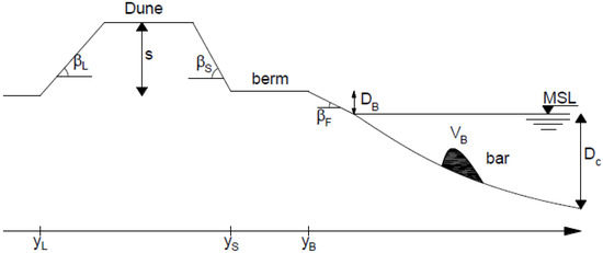
Figure 1.
Cross-shore profile scheme in the CS-Model [8].
Sediment movement along the profile, which alters its geometry, is commonly attributed to wave and wind action, and is influenced by water levels. These changes, which represent the profile’s response, are determined geometrically to maintain mass balance, although the fundamental parameters vary over time.
The CS-Model consists of several integrated modules: two modules for calculating aerial sediment exchange processes (dune erosion and overtopping, as well as aeolian sediment transport) and one module for calculating underwater material exchange (material exchange between the bar and the berm, based on bar theory). A brief explanation of dune erosion and overtopping processes is presented.
The determination of dune erosion is carried out through an analytical model proposed by [10], which is based on the studies of [12,13] on dune erosion. In this model, the eroded volume of the dune is considered to be proportional to the wave impact force hitting its face.
To illustrate the evolution of the profile, a storm impact is considered as an example. If the waves, along with the water level, generate sufficient runup (R), meaning that the wave runup exceeds the base level of the dune, the dune will lose volume (∆VD) and supply sand to the beach berm (Equation (1)). As a consequence of this erosion, the dune’s base shifts inland, and YS decreases, assuming a constant dune slope.
In Equation (1), ∆t represents the time step of the simulation, ZD indicates the vertical distance between the dune toe level and the water level at each time interval (as illustrated in Figure 2), T denotes the wave period, and CS is an empirical impact coefficient, which is based on the analytical dune erosion model proposed by [10], in which the eroded volume is related to the wave runup height and its interaction with the dune face. The coefficient was calibrated using experimental and field data. The smaller the value of ZD, the higher the risk of dune erosion. Additionally, a smaller value of ZD increases the likelihood that waves will reach the upper part of the profile, resulting in R > ZD + S. In this scenario, it is assumed that the wave impact is reduced due to additional overtopping flow over the dune (as expressed in Equation (2)). If the wave runup exceeds the dune crest (i.e., overtopping occurs), the wave energy is assumed to be distributed across the entire dune height. In this case, the eroded volume is no longer proportional to the square of the impact height but instead scales linearly with the product (R − ZD)·S.
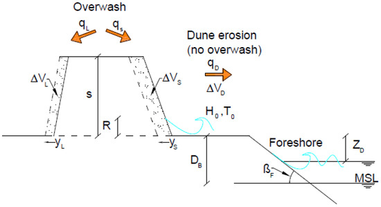
Figure 2.
Diagram of dune erosion and overtopping processes, adapted from [8].
During an overtopping event, the total volume of sediment eroded from the dune due to wave impact (∆VD) is redistributed, with a portion (∆VL) deposited on the landward side of the dune and the remainder (∆VS) transported seaward, resulting in a reduction in YL (i.e., inland displacement). In this case, the slope of the dune’s landward face, represented by βL, is assumed to remain constant. The remaining material is displaced toward the ocean (∆VS). The distribution of ∆VD between ∆VL and ∆VS, the amounts of the eroded dune volume directed landward and seaward, respectively, is determined by the coefficient α (Equation (3)), as expressed by = /(1 + α) and = /(1 + α).
The empirical coefficient A, approximately established as 3 by [14] through a comparative analysis with field data, plays a crucial role. When the variation in sediment volume (∆VD) exceeds the initial volume (VD), it is interpreted as an indication that the dune is undergoing erosive processes, as described by [14].
2.2. Experimental Setup and Flume Characteristics
The hydraulic flume of the Civil Engineering Department at the University of Aveiro, Portugal, has a usable length of 10 m, with a cross-sectional area of 0.40 m × 0.50 m (Figure 3). Based on the limitations of the flume identified in previous studies [15], a geometric scale of 1/40 was adopted. This scale, derived from Froude similarity, was used to construct a model of the cross-shore beach and dune profile.
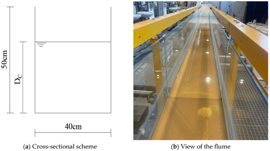
Figure 3.
Hydraulic flume of the Civil Engineering Department (University of Aveiro, Portugal).
A manual wave generator was installed at the upstream end of the flume to produce controlled wave conditions for the experiments. The device operates through pendulum motion and consists of acrylic plates connected to a system of steel shafts. The setup is illustrated in Figure 4.
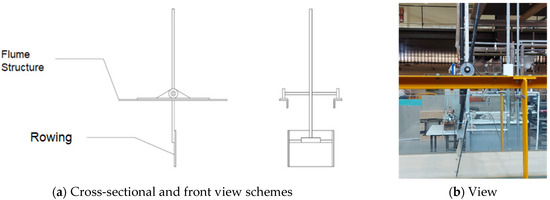
Figure 4.
Wave generation mechanism.
The water supply for the flume is provided by a pumping system. In the context of this study, the flume was kept in a horizontal position and, after adjusting the water level to the desired height, the pumping system was turned off, initiating the tests in the flume.
To evaluate and quantify the characteristics of the waves generated during the tests, an ultrasonic sensor was used (Figure 5). This sensor operates by emitting ultrasonic pulses at intervals of 40 ms, measuring the distance between the sensor and the water surface. The sensor was installed 4.30 m from the wave paddle, in the area near the beach profile.
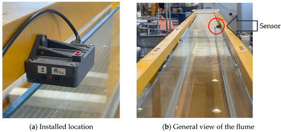
Figure 5.
Ultrasonic sensor for water level measurement.
2.3. Reference Scenario
In this study, the reference scenario (Scenario C0) corresponds to a base beach–dune profile configuration used as a benchmark for both numerical and physical simulations. The term prototype refers to the real-world scale, while the physical model refers to the scaled-down experimental setup (1:40) used in the flume. The CS-Model was applied to both the prototype scale and the scale of the physical model, allowing comparisons across modeling approaches and scales.
Several preliminary tests were carried out with the objective of defining a profile vulnerable to wave attack but without overtopping, so that different reinforcement measures for the profile and their respective performance could later be evaluated. By varying the geometric parameters of the profile and the wave climate, some preliminary conclusions were drawn. In this regard, the profile represented in Figure 6 was considered for the reference scenario with the following values (prototype): 4 m (YL) for the location of the dune toe on the landward side, dune height of 1.5 m, and the position of the dune toe on the seaward side at 16 m (Ys). This position coincides with the berm crest (YB), meaning that the reference profile does not include a berm.
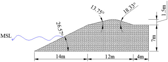
Figure 6.
Profile of the reference scenario at the prototype scale.
For the wave climate, waves perpendicular to the beach were considered, with a wave height (H0) of 2 m. The wave period (T) was calculated as a function of H0 using the following expression [16], resulting in a wave period of 9.34 s:
The beach profile in the physical model was designed to simulate sediment redistribution under wave forcing, with a double-slope configuration and without an initial bar. As highlighted in [9], simplified representations in flume tests are necessary to control variables and ensure repeatability. Therefore, the reference scenario profile assumes a zero volume for the bar. Subsequently, scenarios considering the presence of an initial bar volume are presented. It should be noted that the CS-Model does not simulate the geometry of the bar nor specify its exact position, considering only an available volume of sediments for bar–berm exchanges.
Considering the sediment grain size, as no variations are available in the CS-Model, homogeneous sand was also used in the flume. A representative sample of the sand employed in the physical tests was collected for the purpose of determining the median grain diameter (D50), a critical parameter for the subsequent numerical simulations. Based on the particle size distribution analysis and the construction of the corresponding grading curve, the sand was characterized by a D50 value of 0.40 mm. In both the physical and numerical flume-scale models, the same sediment sample characterized by D50 = 0.40 mm was used to maintain direct comparability. For the prototype-scale numerical simulations, this same value was retained.
2.4. Scenarios Definition
The developed tests aim to characterize the behavior of the beach and dune profile morphology under different conditions of water level, berm width, bar volume, and bar shape. For this reason, values were established for different parameters, which varied independently, while keeping all other variables equal to the reference scenario. The reference scenario corresponds to Scenario C0.
Three scenarios were defined with water surface levels varying between 12 cm, 11 cm, and 10 cm (denoted as Pi, representing the water level in each scenario, as shown in Figure 7a), corresponding to scenarios C0, C1, and C2, respectively. These levels allow for testing a beach profile without a berm for different water surface heights. The selected water levels were also chosen to ensure the required wave height could be generated effectively, while maintaining sufficient depth and preventing wave overtopping during experiments.
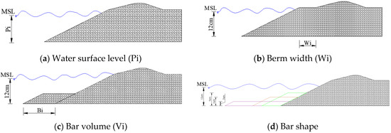
Figure 7.
Schemes of the evaluated scenarios.
To evaluate the berm width, a volume of sand was added to the reference profile, creating a berm with increasing width, with YB values of 50 cm, 62.5 cm, 75 cm, and 87.5 cm, corresponding to scenarios C3, C4, C5, and C6, as shown in Figure 7b. The study of the variation in berm width (Wi) allows the simulation of artificial sand nourishment, enabling inferences about the morphology of profiles under the same wave climate.
For the study of the bar volume’s effect on beach morphology, three scenarios were defined with volumes of 35 cm3/cm, 115.30 cm3/cm, and 196 cm3/cm, corresponding to scenarios C7, C8, and C9, respectively, as shown in Figure 7c. The volume of 35 cm3/cm corresponds to the equilibrium volume of the bar obtained in the CS-Model simulation at the model scale. The volume of 115.30 cm3/cm represents the equilibrium volume of the bar in the reference scenario from the laboratory flume experiment. This volume corresponds to the final bar volume obtained in the CS-Model simulation of the reference scenario (C0) after morphological evolution reached a near-equilibrium condition, characterized by negligible changes in bar geometry over time. However, for the CS-Model simulation of the prototype, the bar volume was 409 cm3/cm, which was considered too large to be represented in the laboratory flume. For this reason, a volume of 196 cm3/cm was considered for scenario C9. For these scenarios, the same bar height of 6 cm was considered, with the bar width (Bi) varying according to each of the mentioned volumes.
Three scenarios were considered to evaluate the bar shape, all with the same bar volume. Thus, scenario C8, defined previously, was used as the reference, with a bar volume of 115.30 cm3/cm. From this, two additional scenarios were defined: C10, with a bar height of 9 cm; and finally, scenario C11, with a submerged bar height of 3 cm (Figure 7d). In these two former scenarios, the width was adjusted to maintain the volume of 115.30 cm3/cm.
The parameters common to all scenarios are presented in Table 1. Table 2 summarizes the parameters considered to evaluate the performance of the beach and dune profile as a function of the water level (scenarios C0 to C2), berm width (scenarios C0 and C3 to C6), berm volume (scenarios C0 and C7 to C9), and berm shape (scenarios C8, C10, and C11).

Table 1.
Beach profile parameters, common to all scenarios.
Table 2.
Defined scenario and beach profile parameters at the physical model scale.
3. Results
This section presents the results obtained from the simulations performed for each of the defined scenarios, followed by an interpretation of the morphological responses observed. At the end of each laboratory experiment (which lasted 6 min), the beach and dune profiles were recorded to assess the morphological changes.
3.1. CS-Model
The CS-Model was used to simulate the same scenarios at both the physical model scale and the prototype scale (1:40 geometric scale) to enable comparison with flume experiments and real-scale behavior. The outcomes are organized by test type, focusing on water level, berm width, bar volume, and profile shape. To facilitate comparison between the physical model and the CS-Model, all values presented here refer to the physical model scale (1:40).
3.1.1. Water Level
Figure 8 shows the final berm position in the CS-Model (i.e., the base of the dune slope and the top of the beach slope) as a function of the water level. At the model scale, all three scenarios (C0 to C2) reached the same value for the final berm position of 38.35 cm, while at the prototype scale, all scenarios resulted in the same value of 20.75 cm. In this context, the term ‘final’ refers to the state of the system at the end of the simulation period.
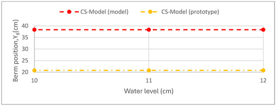
Figure 8.
Final berm position as a function of the water level (scenarios C0 to C2).
It was observed that the numerical model is not sensitive to changes in the water level. In the CS-Model simulations at the prototype scale, a greater retreat of the dune was noted.
Figure 9 shows the time evolution of the berm position, allowing for a comparison between the numerical simulation results. It can be seen that the time evolution of the berm position in the CS-Model is independent of the tested scenario. At the model scale, there is a nonlinear reduction from 40 cm to 38.35 cm, while at the prototype scale, there is also a nonlinear decrease of the berm position, from 40 cm to 20.75 cm.
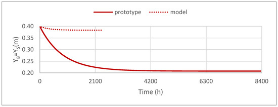
Figure 9.
Evolution of the berm position over time, for scenarios C0 to C2.
3.1.2. Berm Width
For the study of berm width, four scenarios (C3 to C6) were defined with initial berm widths of 10 cm, 22.5 cm, 35 cm, and 47.5 cm. The results from the numerical modeling are shown in Figure 10, which presents the final berm width as a function of the initial berm width. The CS-Model simulation at the model scale for scenarios C0 and C3 to C6 resulted in final berm width values ranging from 0 cm to 45.50 cm. In contrast, the CS-Model at the prototype scale yielded values between 0 cm and 24.13 cm.
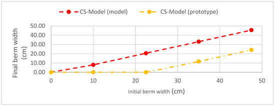
Figure 10.
Berm width as a function of the initial width (CS-Model).
Figure 11 shows the time evolution of the berm width for each scenario (C0 and C3 to C6), based on the calculations performed by the numerical model. In the CS-Model, a nonlinear decrease in berm width over time is observed, tending to converge toward equilibrium. At the model scale, berm width decreased from 10 cm to 8 cm, from 22.50 cm to 20.50 cm, from 35 cm to 33 cm, and from 47.50 cm to 45.55 cm for scenarios C3 to C6, respectively. At the prototype scale, the berm width also decreased from 10 cm to 0 cm, from 22.50 cm to 0 cm, from 35 cm to 11.63 cm, and from 47.50 cm to 24.13 cm, according to scenarios C3 to C6, respectively. Therefore, the variations at the prototype scale are more significant. The results from the CS-Model at the model scale show similar differences from the beginning to the end of the simulation across all scenarios, with the berm width becoming null in scenarios C3 and C4.
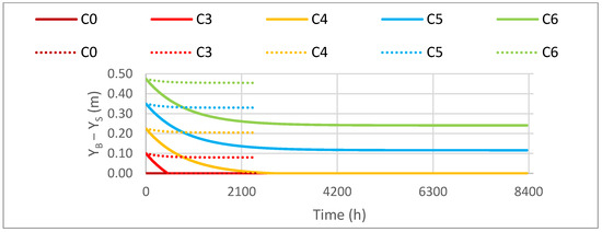
Figure 11.
Evolution of the berm width over time in scenarios C0 and C3 to C6 (CS-Model).
3.1.3. Volume of the Bar
In the study of the bar volume, three scenarios were considered (C7, C8, and C9). The results obtained from the CS-Model at both model and prototype scales are shown in Figure 12, relating the berm position to bar volumes. In the CS-Model, at the model scale, the final position of the berm is 40 cm, 45 cm, and 49.2 cm for scenarios C7 to C9, emphasizing that in these simulations, the beach berm increased in width. For the results of the CS-Model at the prototype scale, the position of the beach berm was 22.40 cm, 26.18 cm, and 29.98 cm, for the respective scenarios C7 to C9. The CS-Model simulations show a linear variation in berm position as a function of bar volume, regardless of the scale (model or prototype).
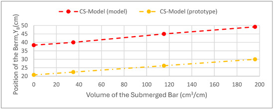
Figure 12.
Evaluation of the volume of the bar in the physical model.
In Figure 13a, the evolution of the berm width over time at the model scale is presented. It is observed that the berm width increases over time, with increasing initial bar volumes, according to scenarios C7 to C9. At the prototype scale (Figure 13b), the wave climate caused a gradual recession of the berm position, resulting in final values of 22.40 cm, 26.18 cm, and 30 cm for scenarios C7, C8, and C9, respectively.
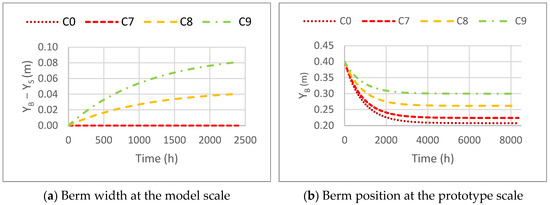
Figure 13.
Evolution of the berm width and position over time in the CS-Model, for scenarios C0 and C7 to C9.
It is observed that the CS-Model, at the model scale, created a berm for scenarios C8 and C9, while in scenario C7, there was virtually no change in the morphology, because the volume corresponding to the smallest bar in these scenarios is equal to the equilibrium volume of the bar. It was noted that at the prototype scale, the equilibrium volume of the bar is higher than the volume considered in the three scenarios. Therefore, in this situation, the trend is for the beach and/or dune to lose material to the bar until the equilibrium volume of the bar is reached. For this reason, in the CS-Model simulations at the prototype scale, there was always a recession in the dune.
3.1.4. Bar Shape
To analyze the shape of the bar, three scenarios were considered (C8, C10, and C11). The results from scenario C8 were presented in the previous section and serve as a reference for the simulations of the other bar shapes. In the numerical simulations using the CS-Model, it is not possible to reproduce the exact shape of the bar, because the model defines the bar only through its volume, VB. Thus, the results and values of the CS-Model for both the model scale and the prototype scale are presented in Figure 14. For the CS-Model at the model scale, the final berm position is 45 cm, implying a gain in material for the beach berm. However, for the CS-Model at the prototype scale, the final berm position is 26.18 cm, resulting in a recession of the berm position.
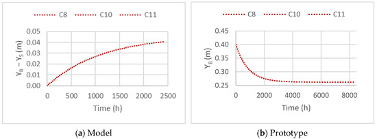
Figure 14.
Evolution of the berm width and position over time in the CS-Model for scenarios C8, C10, and C11.
Figure 14a presents the time evolution of the berm width, representing the result of the CS-Model at the model scale for the three scenarios (C8, C10, and C11), while Figure 14b presents the time evolution of the berm in the CS-Model at the prototype scale, with the berm position varying from 40 cm to 26.18 cm.
3.2. Flume Tests Results Assessment
Laboratory tests were carried out for the same scenarios defined in the numerical simulations, allowing for a comparison between physical and numerical results. The results are organized by test type—with particular focus on the profile shape—water level, as well as the bar volume, position, and crest depth.
Throughout the experiments, in order to record the evolution of the beach profile, a grid of vertical lines spaced 2 cm apart was drawn on the side wall of the flume. This setup facilitated the measurement of the sand surface elevation at the end of each time step using a ruler graduated in millimeters. No significant sediment loss occurred during the experiments; therefore, the discrepancies in volume measurements are attributed to the limitations of the measurement method.
3.2.1. Water Level
To assess the morphological effects observed in tests C0 to C2, Figure 15 presents the final beach and dune profiles recorded at the end of each laboratory experiment.
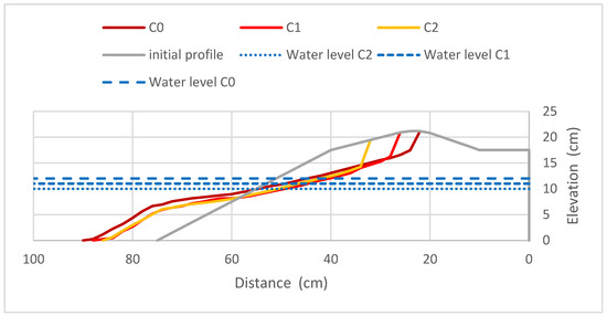
Figure 15.
Final profile morphology for scenarios C0 to C2.
Throughout the tests, it was observed that the sand gradually migrated downward along the profile, with the erosion volume defined as the area below the initial profile. Simultaneously, a bar forms in the lower section of the profile (area above the initial configuration), considered as the deposition volume. The morphology of each test, at each one-minute time step, was compared to the reference scenario profile, enabling the quantification of the volumes corresponding to the erosion and accretion zones, as presented in Table 3.
Table 3.
Erosion and deposition volume, as well as the absolute and relative differences in profile volumes, for scenarios C0 to C2 of the laboratory tests.
Upon analyzing Table 3, it was observed that almost all the relative difference percentages are below 10%, a condition sufficient to ensure mass conservation in the profile during the laboratory experiments. In scenario C1, a slight decrease in the bar area was observed between the 5th and 6th minutes. This behavior is believed to be related to a reduced measurement precision, as all other results indicate a progressive evolution toward equilibrium.
The scenario with the lowest water level, corresponding to scenario C2, shows the smallest morphological variations. Scenario C1, in turn, presents the highest erosion volume, with 11.66 × 10⁻³ m3/m, while scenario C0 reveals the highest deposition volume, approximately 11.53 × 10⁻³ m3/m. In scenario C1, beach and dune erosion were more significant, while in scenario C0, dune erosion was greater than in the other scenarios. In all scenarios, the largest morphological variation occurred within the first 60 s. During the first 60 s, the erosion rates of 46.83%, 56.50%, and 69.54%, as well as the accretion rates of 55.14%, 79.14%, and 68.85%, respectively, were observed for scenarios C0, C1, and C2 when compared to the final situation of the test.
Figure 16 shows the variation over time in the depth and position of the bar crest in scenarios C0 to C2. The bar crest was identified as the inflection point of the bar shape, characterized by the change in the slope of the upper face of the submerged profile.
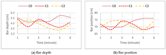
Figure 16.
Variation in bar depth and position over time, for scenarios C0 to C2.
In this regard, Figure 17 shows the position of the final berm (base of the dune slope and top of the beach slope) as a function of the water level. Thus, the physical model results are situated between 23.97 cm and 33.25 cm.
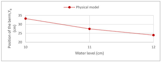
Figure 17.
Final position of the berm, depending on the water level.
In Figure 18, it is observed that the temporal evolution of the berm position in the physical model is less pronounced as the water level decreases. It is also noted that the position of the seaward base of the berm is directly proportional to the water surface level, showing smaller retreats as the water level decreases.
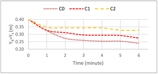
Figure 18.
Evolution of the berm position, for scenarios C0 to C2, over time.
3.2.2. Berm Width
For the study of berm width, four scenarios (C3 to C6) were defined with the following berm widths: 10 cm; 22.5 cm; 35 cm; and 47.5 cm. Figure 19 represents the morphology of each laboratory test at the end of six minutes, thus allowing the observation of the effect of increasing berm width. It should be noted that the greater the initial berm width, the smaller the retreat of the dune toe position at the end of the test, and consequently, the smaller the erosion caused to the dune.
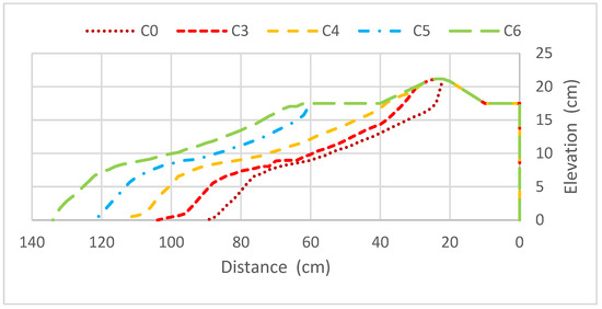
Figure 19.
Profile morphology at the end of the laboratory tests, for scenarios C0 and C3 to C6.
Table 4 presents the erosion and deposition volume for each berm width scenario, minute by minute.
Table 4.
Erosion and deposition volume, as well as the absolute and relative differences in profile volumes, for scenarios C3 to C6 from the laboratory tests.
In scenario C4, a slight decrease in the bar volume was observed in the last minute of the test. It is noteworthy that, regardless of the berm width, the final bar volume ranges from 10.56 to 10.90 × 10⁻³ m3/m, indicating a trend that suggests the formation of the bar is not dependent on the berm width. It is also relevant to note that the greatest erosions occur in scenarios C3 and C4, because the dune is directly affected by wave action, while in scenarios C5 and C6, the berm is sufficiently wide, preventing dune erosion, and the final erosion volume is lower than in C3 and C4.
Figure 20 shows the variation over time in bar depth and position for scenarios C0 and C3 to C6. In Figure 20a, it is observed that the bar crest depth is independent of the amount of material used, displaying an oscillatory behavior over time, which tends to converge to the same value of 5.35 cm at the end of the test. In Figure 20b, it is observed that the bar position is directly proportional to the berm width, with larger berm widths corresponding to a further offshore bar crest position.
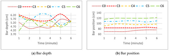
Figure 20.
Variation in bar depth and position over time, for scenarios C0 and C3 to C6.
The results of the physical model are shown in Figure 21, where the final berm width is presented as a function of the initial berm width. The physical model shows final berm widths ranging from 0 cm to 22 cm.
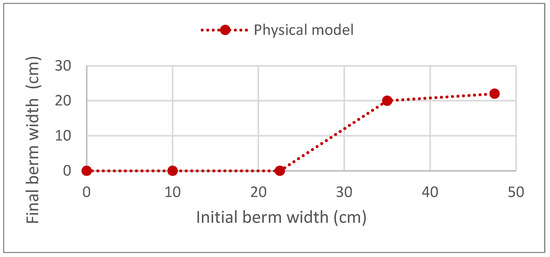
Figure 21.
Berm width as a function of initial berm width (physical model).
Figure 22 presents the temporal evolution of berm width for each scenario (C0 and C3 to C6) of the laboratory tests.
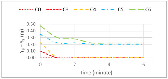
Figure 22.
Evolution of berm width over time, for scenarios C0 and C3 to C6 (physical model).
Upon analyzing the laboratory tests, it was observed that the results for scenarios C3 and C4 are quite similar, with final berm position (YB) values of 33.25 cm and 38.33 cm, respectively. Both of these scenarios resulted in dune erosion, with scenario C3 showing a higher erosion rate. Therefore, it can be stated that increasing the berm width was beneficial for better dune shape preservation. In scenarios C5 and C6, the dune was preserved as the erosion did not affect the dune, with wave energy dissipating along the berm. Additionally, in these two scenarios, a residual berm width was maintained. At the end of the tests for scenarios C5 and C6, the berm position was 60 cm and 62 cm, resulting in final berm widths of 20 cm and 22 cm, respectively.
3.2.3. Volume of the Bar
In the study of the bar volume, three scenarios were considered: C7, C8, and C9. After obtaining the morphological evolution of the conducted tests, it was possible to represent their morphology at the end of the test (Figure 23).
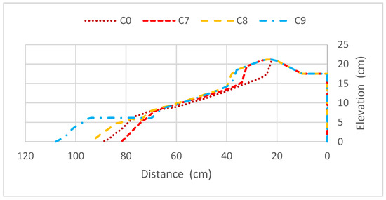
Figure 23.
Profile morphology at the end of the test, for scenarios C0 and C7 to C9.
Based on the morphological evolution recorded throughout the tests, it was possible to determine the erosion and deposition volumes resulting from sediment dynamics for each minute of the tests performed (Table 5). It is observed that adding an initial volume to the bar improved dune preservation compared to the reference scenario, C0. However, in scenarios C7, C8, and C9, erosion on the dune still occurred. The values obtained for the dune toe position at the end of their respective tests were 32.92 cm, 37.90 cm, and 36.57 cm, respectively. Therefore, the smallest bar volume, scenario C7, corresponds to the greatest dune erosion. However, despite scenario C8 having a smaller bar volume than scenario C9, it resulted in better dune preservation than scenario C9.
Table 5.
Erosion and deposition volume, as well as the absolute and relative differences in the volumes on the profile, for scenarios C7 to C9 of the laboratory tests.
In scenarios C7 and C9, a slight decrease in the erosion volume was observed in the last minute of the test, showing some stability in the behavior, which tends to converge towards equilibrium. In Figure 24, it can be seen that the initial bar volume caused the initial position and depth of the crest to differ, but they tend to evolve towards the same final result, with the exception of just one scenario, C0, which corresponds to the reference scenario.
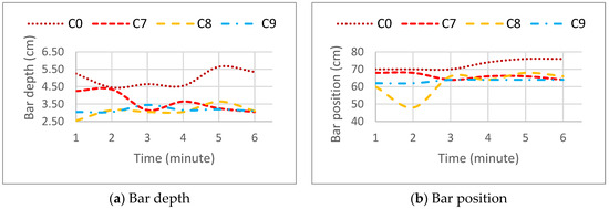
Figure 24.
Variation in depth and position of the bar over time for scenarios C0 and C7 to C9.
The laboratory test results for C0 and C7 to C9 are presented in Figure 25, relating the berm position to the bar volumes.
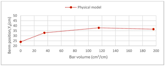
Figure 25.
Evaluation of the bar volume in the laboratory model.
3.2.4. Bar Shape
To analyze the shape of the bar, three scenarios were considered: C8, C10 and C11. The results for scenario C8 were presented in the previous section and serve as a reference for the tests involving other bar shapes. Figure 26 depicts the morphology of each of these scenarios at the final stage of the laboratory tests, illustrating how the shape of the bar can influence the profile morphology.
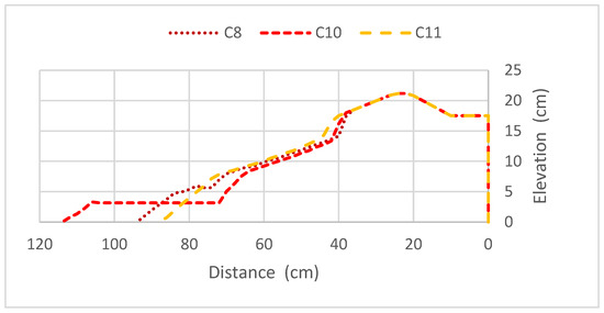
Figure 26.
Profile morphology at the end of the test, for scenarios C8, C10, and C11.
Based on the morphology of each test, it was possible to determine the erosion and deposition volume over time (Table 6).
Table 6.
Erosion and deposition volume, as well as the absolute and relative differences in the volumes on the profile, for scenarios C10 and C11 of the laboratory tests.
In scenario C11, the morphological changes over time were reduced, suggesting that the initial bar shape is closer to the equilibrium, thereby minimizing sediment dynamics. Similarly to scenario C8, scenarios C10 and C11 showed improved dune conservation compared to the reference scenario, C0. The final values of the berm position (YB) were 37.9 cm, 38.53 cm, and 40 cm for scenarios C8, C10, and C11, respectively. It was observed that scenario C10, despite having a lower bar height, exhibited a lower erosion rate than scenario C8. However, in both scenarios (C8 and C10), erosion slightly affected the dune. Therefore, among these scenarios, only scenario C11 ensures dune conservation, as erosion did not impact the dune at any point. Figure 27 further confirms that scenario C11 exhibits reduced sediment dynamics, maintaining the bar crest position and corresponding depth constant over time.
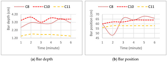
Figure 27.
Variation in bar depth and position over time, for scenarios C8, C10, and C11.
4. Discussion
This section presents a critical analysis of the results from the numerical simulations and laboratory tests. A comparison of the performance of the CS-Model at both prototype and model scales is discussed, aiming to better understand the coastal erosion processes, particularly the interactions among the beach profile, dune system, and bar.
The study demonstrated that the CS-Model is not sensitive to variations in water level, as the results were identical for different water levels in scenarios C0 to C2. This behavior may be attributed to the simplification of boundary conditions in the numerical model, which does not account for dynamic variations in water levels, unlike sandy beaches associated with coastal dunes models that integrate tides and other factors [3]. Moreover, dune retreat was more pronounced in the CS-Model at the prototype scale, indicating an overestimation of erosion. This is likely due to the lack of variability in erosive processes, such as the interaction between water and sediments [3]. According to [17], an increase in the water surface level amplifies the interaction between waves and the beach profile, accelerating erosion. The results of this study confirm this trend, with scenario C1, which features a higher water level, causing greater erosion in the upper part of the beach.
It was observed that a greater berm width acts as a buffer, reducing dune and beach erosion, especially in scenarios C5 and C6. However, the simulations at model and prototype scales showed differences in berm width variations. These discrepancies can be explained by the CS-Model’s limitation in simulating the dynamics of water and sediment transport in the berm interaction zone [18]. The relationship between berm width and the reduction in dune erosion is well documented, as shown by [19]. This study supports these findings, demonstrating that a wider berm results in the dissipation of wave energy, preventing dune erosion. In scenarios C5 and C6, berm width was crucial for dune protection, which is consistent with the results of other authors [8,18].
In scenarios C7 to C9, at the model scale, an increase in the bar volume resulted in an expansion of the berm width, indicating material deposition on the beach. However, in the prototype, continuous dune erosion was observed, suggesting that the equilibrium volume of the bar in the prototype exceeds the volume used in the model-scale simulations. This highlights the inadequacy of model-scale simulations in accurately replicating real coastal system conditions [20]. Previous studies, such as those by [21], suggest that the volume of the bar can mitigate dune erosion, albeit with diminishing returns, as the volume increases. The laboratory tests confirm that, although the increase in bar volume, as observed in scenarios C8 and C9, reduces dune erosion, this relationship is not linear. The analysis suggests that an optimized adjustment of bar volume could lead to more effective and cost-efficient solutions.
Sediment properties and scale effects may have impact on physical–numerical discrepancies. These issues have been previously highlighted by [9,10], who emphasized the challenges in reconciling laboratory-scale and prototype-scale behaviors in beach and dune morphodynamic modeling. The CS-Model only uses a single sediment grain size to characterize all the beach profile, from the submerged part to the dune. As discussed in [22], geometric similarity alone does not ensure dynamic similarity in sediment transport processes, particularly given the nonlinear dependence of critical shear stress and transport rates on grain size. While geometric and hydraulic scaling were respected, the sediment grain size (D50 = 0.40 mm) was held constant across all model scenarios due to the limitations of the CS-Model. This approach simplifies the setup but introduces potential scale effects. As demonstrated by [22], the sediment transport response is highly sensitive to grain size, especially in shallow flows where incipient motion thresholds and bedform evolution are strongly grain-dependent. Furthermore, sediment-related scale effects do not follow a linear law, making direct comparison between physical and prototype results subject to distortion. Therefore, morphodynamic results obtained from prototype-scale simulations should be interpreted cautiously, recognizing that sediment transport rates and erosion/deposition patterns may be over- or underestimated due to the fixed sediment size assumption. Despite this limitation, relative patterns remain valid, particularly when used for qualitative assessments or scenario comparisons.
The CS-Model does not account for the shape of the bar, relying solely on its volume. This limitation restricts the model’s ability to accurately simulate the morphological interactions between waves, currents, and sediments, which are crucial for beach evolution and dune protection [4,23]. In the physical model, the shape of the bar, in terms of height and width, also plays a key role in wave energy dissipation. Borsje et al. [21] highlights the importance of these factors, which is confirmed in this study. The results indicate that the difference between the water level and the height of the bar affects energy dissipation, with the width of the bar becoming more significant in dune protection than its height, when this difference reaches 6 cm.
One limitation of the current modeling approach is the assumption of constant dune face slopes (βL and βS) throughout the simulation. In reality, dune slopes may evolve due to variations in sediment characteristics (grain size, for instance), sediment transport, and erosional processes. Main conclusions of the developed work apply only under the tested conditions and sediment types and should not be generalized to full-scale applications of the CS-Model. Future works can explore models that allow for dynamic adjustment of dune slopes to better represent morphological responses under varying wave conditions.
5. Conclusions
This study addressed a relevant gap in coastal engineering research by systematically comparing the effectiveness of different artificial nourishment strategies under controlled laboratory and numerical conditions. While many previous studies have investigated berm widening and bar reinforcement individually, few have directly compared them using a consistent experimental framework at multiple scales. The scenarios explored here were designed to provide new insights into how variations in berm width and bar volume and shape, as well as influence beach morphological changes and dune erosion, supporting more effective and targeted coastal protection strategies.
Simulations of the CS-Model at the model scale resulted in dune retreat values lower than those obtained in simulations at the prototype scale, as evaluated by the berm position. In evaluating the effect of the bar volume in the CS-Model simulations, it is important to note the equilibrium bar volume. At the model scale, as the bar volume increased, the position of the beach berm increased due to the fact that the 35 cm3/cm volume is greater than the equilibrium bar volume. Whenever the initial bar volume exceeds the equilibrium bar volume, the bar volume decreases, and this material moves toward the beach, increasing the beach width. On the other hand, in the three scenarios of the bar volume study at the prototype scale, dune erosion was always observed. The equilibrium volume of the bar in the prototype is approximately 409 cm3/cm, while the volumes considered in the studied scenarios were lower. In this situation, an increase in the bar volume was observed, leading to the material moving towards the bar, resulting in beach and dune erosion. The CS-Model only considers the bar volume, making this parameter independent of the shape and position of the bar. Thus, for the same bar volume, the result obtained is always the same.
In all the laboratory tests, the highest profile variation rates, resulting in accretion on the bar and erosion in the upper part of the profile, occurred during the first 60 s, with changes exceeding 40% of the total morphological variation recorded at the end of the test. In evaluating the effect of the water surface level in the physical model, a higher rate of dune erosion variation was recorded for scenario C0, while scenario C2 exhibited a lower rate of dune erosion variation. Thus, it can be concluded that the lower the water surface height, the less likely the wave climate will cause dune erosion. Regarding the berm width’s influence, it was found that the wider the berm, the lower the chances of dune erosion occurring, as the beach width contributes to wave energy dissipation. When the width is sufficient in dissipating wave energy, no dune erosion occurs, and only a reduction in berm width is observed, as confirmed in scenarios C5 and C6. For the evaluation of the bar volume in the laboratory, the scenarios suggest that increasing the bar volume, although beneficial in reducing dune erosion, does not necessarily guarantee the most effective solution when applied in isolation or without optimization of other parameters, as seen in the results from scenarios C8 and C9. The relationship between bar volumes and dune erosion reduction is not linear, which suggests that studying the bar volume for dune erosion mitigation could lead to a more optimized artificial nourishment project, requiring fewer financial resources. During the laboratory tests, it was observed that for the same bar volume, when the difference between the water surface level and the bar height is at least 3 cm (scenario C10), the height of the bar becomes more crucial in dissipating wave energy. If this difference exceeds 6 cm (scenario C8), the width of the bar becomes more important than the height of the bar, leading to improved dune erosion mitigation. Therefore, scenario C11, with a 3 cm bar height, yielded better results in dune shape preservation than scenario C8, which had a height of 6 cm.
In conclusion, the laboratory tests showed that artificial nourishment involving bar volume was more effective at mitigating dune erosion than those focused on increasing berm width. Notably, only scenario C11 fully preserved the dune. These findings may offer valuable preliminary guidance for future artificial nourishment projects, contributing to more effective and sustainable coastal management.
Author Contributions
Conceptualization, C.C. and M.L.; Methodology, C.C. and M.L.; Software, A.S.; Validation, A.S. and C.C.; Formal analysis, A.S.; Writing—original draft, A.S.; Writing—review and editing, C.C. and M.L.; Supervision, C.C. and M.L. All authors have read and agreed to the published version of the manuscript.
Funding
This research received no external funding.
Data Availability Statement
The original contributions presented in this study are included in the article. Further inquiries can be directed to the corresponding author.
Conflicts of Interest
The authors declare no conflicts of interest.
References
- D’Alessandro, F.; Tomasicchio, G.R.; Frega, F.; Leone, E.; Francone, A.; Pantusa, D.; Barbaro, G.; Foti, G. Beach–Dune System Morphodynamics. J. Mar. Sci. Eng. 2022, 10, 627. [Google Scholar] [CrossRef]
- Larson, M.; Palalane, J.; Fredriksson, C.; Hanson, H. Simulating cross-shore material exchange at decadal scale. Theory and model component validation. Coast. Eng. 2016, 116, 57–66. [Google Scholar] [CrossRef]
- Marinho, B.; Coelho, C.; Larson, M.; Hanson, H. Simulating cross-shore evolution towards equilibrium of different beach nourishment schemes. Proc. Coast. Dyn. 2017, 2017, 15. [Google Scholar]
- Masselink, G.; Hughes, M.; Knight, J. Introduction to Coastal Processes and Geomorphology; Routledge: London, UK, 2014. [Google Scholar]
- Roelvink, D.; Reniers, A.; van Dongeren, A.; van Thiel de Vries, J.; McCall, R.; Lescinski, J. Modelling storm impacts on beaches, dunes and barrier islands. Coast. Eng. 2009, 56, 1133–1152. [Google Scholar] [CrossRef]
- DHI MIKE 21. User Manual; DHI Water & Environment: Singapore, 2012. [Google Scholar]
- Guimarães, A.; Coelho, C.; Veloso-Gomes, F.; Silva, P.A. 3D Physical Modeling of an Artificial Beach Nourishment: Laboratory Procedures and Nourishment Performance. J. Mar. Sci. Eng. 2021, 9, 613. [Google Scholar] [CrossRef]
- Marinho, B. Artificial Nourishments as a Coastal Defense Solution: Monitoring and Modelling Approaches. Ph.D. Thesis, Universidade de Aveiro, Aveiro, Portugal, 2018. [Google Scholar]
- D’Alessandro, F.; Tomasicchio, G.R. Wave–dune interaction and beach resilience in large-scale physical model tests. Coast. Eng. 2016, 116, 15–25. [Google Scholar] [CrossRef]
- Larson, M.; Erikson, L.; Hanson, H. An analytical model to predict dune erosion due to wave impact. Coast. Eng. 2004, 51, 675–696. [Google Scholar] [CrossRef]
- Vitousek, S.; Barnard, P.L.; Limber, P.; Erikson, L.; Cole, B. A model integrating longshore and cross-shore processes for predicting long-term shoreline response to climate change. J. Geophys. Res. Earth Surf. 2017, 122, 782–806. [Google Scholar] [CrossRef]
- Fisher, J.S.; Overton, M.F.; Chisholm, T. Field Measurements of Dune Erosion. In Coastal Engineering 1986; American Society of Civil Engineers: Reston, VA, USA, 1987; pp. 1107–1115. [Google Scholar]
- Nishi, R.; Kraus, N. Mechanism and calculation of sand dune erosion by storms. In Proceedings of the 25th Coastal Engineering Conference, American Society of Civil Engineers (ASCE), Orlando, FL, USA, 2–6 September 1996; pp. 3034–3047. [Google Scholar]
- Larson, M.; Donnelly, C.; Jiménez, J.A.; Hanson, H. Analytical model of beach erosion and overwash during storms. Proc. Inst. Civil. Eng.-Marit. Eng. 2009, 162, 115–125. [Google Scholar] [CrossRef]
- Vale, D.; Pires, R. Avaliação do Espraiamento e Galgamento em Estruturas Costeiras. Projeto de Licenciatura em Engenharia Civil. Não Publicado. Universidade de Aveiro, Aveiro, Portugal, 2022. (In Portuguese). [Google Scholar]
- Coelho, C. Riscos de Exposição de Frentes Urbanas para Diferentes Intervenções de Defesa Costeira. Ph.D. Thesis, Universidade de Aveiro, Aveiro, Portugal, 2005. (In Portuguese). [Google Scholar]
- van Rijn, L.C.; Tonnon, P.K.; Walstra, D.J.R. Numerical modelling of erosion and accretion of plane sloping beaches at different scales. Coast. Eng. 2011, 58, 637–655. [Google Scholar] [CrossRef]
- Puleo, J.A.; Lanckriet, T.; Conley, D.; Foster, D. Sediment transport partitioning in the swash zone of a large-scale laboratory beach. Coast. Eng. 2016, 113, 73–87. [Google Scholar] [CrossRef]
- Ferreira, A.M.; Coelho, C.; Silva, P.A. Medium-Term Effects of Dune Erosion and Longshore Sediment Transport on Beach–Dune Systems Evolution. J. Mar. Sci. Eng. 2024, 12, 1083. [Google Scholar] [CrossRef]
- Van Rijn, L.C.; Tonnon, P.K.; Sánchez-Arcilla, A.; Cáceres, I.; Grüne, J. Scaling laws for beach and dune erosion processes. Coast. Eng. 2011, 58, 623–636. [Google Scholar] [CrossRef]
- Borsje, B.W.; van Wesenbeeck, B.K.; Dekker, F.; Paalvast, P.; Bouma, T.J.; van Katwijk, M.M.; de Vries, M.B. How ecological engineering can serve in coastal protection. Ecol. Eng. 2011, 37, 113–122. [Google Scholar] [CrossRef]
- Raquel, S. Avaliação Experimental e Numérica de Parâmetros Associados a Modelos de Evolução da Linha de Costa. Ph.D. Thesis, Universidade do Porto, Porto, Portugal, 2010. (In Portuguese). [Google Scholar]
- Chun, I.; Lim, H.S.; Shim, J.S.; Park, K.S. Numerical Analysis of the Performance of Perforated Coastal Structures under Irregular Wave Conditions. J. Coast. Res. 2015, 315, 1159–1169. [Google Scholar] [CrossRef]
Disclaimer/Publisher’s Note: The statements, opinions and data contained in all publications are solely those of the individual author(s) and contributor(s) and not of MDPI and/or the editor(s). MDPI and/or the editor(s) disclaim responsibility for any injury to people or property resulting from any ideas, methods, instructions or products referred to in the content. |
© 2025 by the authors. Licensee MDPI, Basel, Switzerland. This article is an open access article distributed under the terms and conditions of the Creative Commons Attribution (CC BY) license (https://creativecommons.org/licenses/by/4.0/).