Article

Bayesian Framework for Detecting Changes in Downstream Flow–Duration Curves Induced by Reservoir Operation Method

1
School of Civil, Environmental and Architectural Engineering, Korea University, Seoul 02841, Republic of Korea
2
Department of Civil Engineering, Dong-A University, Busan 49315, Republic of Korea
*
Author to whom correspondence should be addressed.
Water 2025, 17(14), 2078; https://doi.org/10.3390/w17142078
Submission received: 2 June 2025 / Revised: 5 July 2025 / Accepted: 8 July 2025 / Published: 11 July 2025

Abstract

The construction of a dam significantly alters downstream flow characteristics, often analyzed through changes in flow–duration curves before and after construction. Typically, post-dam flow–duration curves exhibit increased probabilities in low-flow zones and decreased probabilities in high-flow zones, primarily influenced by reservoir operation methods (ROMs). This study introduces a Bayesian framework to replace ROM simulations for predicting downstream flow–duration curve changes after dam construction, mainly during the flood season. Within this framework, inflow data are treated as random variables, and the ROM is analogized to a likelihood function in Bayesian analysis. The key challenge lies in deriving a likelihood function that mimics the given ROM. The Rigid ROM, a hybrid of constant rate and constant magnitude ROMs commonly used in the Republic of Korea, is targeted in this study. Using hourly inflow data from the Republic of Korea’s Andong Dam (2010–2019), the proposed Bayesian method produces flow–duration curves closely matching simulation-based results, validating its accuracy. Furthermore, the method’s ability to seamlessly handle multi-dam systems in a series highlights its practical advantage, attributed to the iterative nature of Bayesian updates. This study underscores the Bayesian approach’s potential for efficient and robust flow–duration curve modeling in complex hydrological systems.

1. Introduction

Changes in flow–duration characteristics are a significant consequence of dam construction by modifying the timing, magnitude, and frequency of both minimum and maximum flows. Previous studies have consistently reported significant changes in flow–duration curves—a cumulative frequency representation indicating the percentage of time specific discharge levels are equaled or exceeded—highlighting increased frequencies of low flows and diminished occurrences of high flows. These shifts contribute to substantial modifications in seasonal flow regimes [1,2,3,4]. In addition, dams act as sediment traps, substantially decreasing the transport of suspended sediments to downstream areas [5]. These disruptions in sediment continuity have far-reaching consequences for downstream river morphology, water quality, and aquatic ecosystems [6]. For instance, Wang et al. [2] observed these effects in the Yangtze River following the construction of the Three Gorges Dam. Similarly, Magilligan and Nislow [3] analyzed data from 21 dams across the United States and identified comparable trends. Studies in the Republic of Korea have also corroborated these findings [7,8,9,10,11]. These changes are typically detected through comparative analyses of observed flow data from pre- and post-dam construction periods or by simulating flow dynamics based on reservoir operation strategies for newly designed dams.
Traditionally, analyses of flow–duration curves before and after dam construction have primarily emphasized the potential reduction in flood risks and improvements in low-flow conditions. However, given the profound impacts of dams on the physical, chemical, and ecological characteristics of river systems, the evaluation of altered flow–duration curves has gained increasing importance [12]. Low-flow conditions play a pivotal role in water quality management, while high-flow frequency significantly influences sediment transport and aquatic ecosystem dynamics [13,14]. Consequently, a more comprehensive approach to flow–duration analysis is required, as traditional methods focusing solely on flood control and water supply management may no longer suffice. This complexity is further exacerbated in scenarios involving multiple dams, where diverse stakeholders with varying priorities are involved. Thus, there is a pressing need for a flexible and efficient methodology to derive flow–duration curves that can promptly accommodate changes in reservoir operation rules across one or multiple dams.
The detection of potential changes in downstream flow–duration following dam construction necessitates the implementation of reservoir operation simulations. Reservoir operation involves determining dam outflows based on dam inflow data, highlighting its critical influence on downstream hydrological patterns. The specific outflow patterns are intrinsically shaped by the chosen reservoir operation method (ROM), which in turn significantly impacts the morphology of the runoff hydrograph in downstream channels [15,16]. Furthermore, the ROM plays a pivotal role in flood risk management, underscoring its importance in the context of water resource planning and mitigation strategies [17,18]. In essence, the relationship between dam inflow and outflow is fundamentally causal, mediated by the ROM, which acts as a critical determinant of downstream hydrological outcomes.
Various types of ROMs are employed in the Republic of Korea, including the Auto ROM, Rigid ROM, and Technical ROM [19,20,21]. The Auto ROM operates by restricting outflows until the water level drops below the target level, releasing all inflows only when the water level exceeds the target. Consequently, the reservoir water level is maintained at or below the target level. The Rigid ROM, often referred to as the constant rate and constant magnitude method, determines outflows by applying a fixed proportion to the inflow until the peak inflow is reached. After the peak inflow, a pre-determined constant magnitude of outflow is maintained, releasing all inflows only when they fall below the constant magnitude. In contrast, the Technical ROM releases a fixed magnitude of outflow only when the reservoir storage exceeds the flood control volume [22]. Among these methods, the Rigid ROM is the most commonly implemented [19,20,21] in the Republic of Korea. Notably, 13 out of 19 multi-purpose dams in the country currently adopt the Rigid ROM as their primary operational method [22,23].
Even though the Bayesian method has been extensively utilized in reservoir operation research [24,25,26,27], this study highlights the potential of leveraging the Bayesian method to address the causal relationship inherent in reservoir operation. Distinct from earlier works, this study aims to demonstrate that the ROM can be fundamentally substituted with the Bayesian framework. As previously discussed, the ROM functions as a procedure that modifies inflow data to produce outflow data. By treating dam inflow as a random variable characterized by a probability distribution function (PDF), the corresponding PDF of dam outflow can be derived through consideration of the ROM. This process closely parallels the Bayesian framework, where the PDF of inflow data represents the prior distribution—reflecting initial assumptions or uncertainty about the system before incorporating new observations. The ROM serves as the likelihood function, quantifying the probability of observing specific outcomes given the assumed inflow conditions. Consequently, the derived outflow PDF can be interpreted as the posterior distribution, representing the updated belief about the system’s behavior after accounting for the operational rules imposed by the ROM. Given its straightforward application, the Bayesian method offers an efficient alternative to simulation-based ROM applications. Specifically, the PDF of dam outflow can be derived by applying the Bayesian method to inflow data using the specified ROM. However, a key challenge remains: the ROM must be represented in a form compatible with a likelihood function.
This study aims to simplify the derivation of downstream flow–duration curves altered by dam construction by employing a Bayesian approach in place of ROMs in flood seasons. By using the Bayesian method, the PDF of dam outflow is derived through the integration of the inflow data PDF and a likelihood function corresponding to a specific ROM. This approach not only facilitates the derivation of downstream runoff characteristics but also aids in detecting potential changes in flow–duration curves post-dam construction.
In this study, the Rigid ROM, the most prevalent method in the Republic of Korea, is selected as the target ROM, with full consideration of the roles of its components: constant rate ROM and constant magnitude ROM. The theoretical framework encompasses a general introduction to the Bayesian method and the derivation of likelihood functions for the Rigid ROM. The Andong Dam in the Republic of Korea serves as a case study. The Bayesian method is applied to 2019 inflow data to evaluate its applicability to the Rigid ROM, with the results validated against simulation outputs. Additionally, the downstream flow–duration changes are analyzed using data from 2010 to 2019, providing insights into the effects of dam operation on downstream flow–duration. The proposed Bayesian approach is also extended to multi-dam scenarios, showcasing its adaptability for complex reservoir operations.

2. Methodology

2.1. Bayesian Framework

The Bayesian method is used to obtain the posteriori probability, by combining the priori probability with the likelihood function [28,29]. The priori probability indicates the probability of a specific parameter before obtaining the observational information, while the likelihood function is the conditional probability of observing the additional data under the condition of the specific parameter. The priori probability is updated to the posteriori probability by considering the additional information as a form of the likelihood function.
In the Bayesian method, the posteriori probability is calculated based on the total probability theorem. That is, the posteriori probability is calculated as the total probability with respect to the likelihood function and the priori probability. The posteriori probability is calculated by the following equation [30]:
P θ ε = L ( ε | θ ) π ( θ ) L ( ε | θ ) π ( θ ) d θ
where π ( θ ) is the priori probability of the parameter θ , L ( ε | θ ) is the likelihood function, and P ( θ | ε ) is the posteriori probability updated by considering the new information. The denominator in this equation is the total probability of the likelihood function and the priori probability, which normalizes the posteriori probability distribution. The normalization converts the sum of the posteriori probability to unity. Equation (1) can also be expressed rather simply, as follows:
P θ ε = k L ( ε | θ ) π ( θ )
where k is the normalization factor that is the reciprocal of the total probability according to the denominator of Equation (1).
In this study, the posteriori probability was calculated by the equation in a discrete format. Also, to transform the continuous distribution into a discrete one, it was necessary to replace the continuous parameter θ with the discrete parameter θ i . The discrete Bayesian approach utilizes probability mass functions and numerical computation of the theorem. This necessitates discretization of the parameter space into uniform intervals ( θ ), with Equation (3) calculated for each discrete segment θ i . The selected θ must ensure that the discrepancy between continuous and discrete results remains within acceptable bounds; thus, the discrete approximation can be regarded as valid and reliable. The basic equation form of the discrete Bayesian method is as follows:
P θ i ε i θ = L ε i θ i π ( θ i ) θ i = 1 n L ε i θ i π ( θ i ) θ
where P ( θ | ε ) is the posteriori probability of the discrete parameter θ i , L ε i θ i is the likelihood function, and π ( θ i ) is the priori probability.

2.2. Determination of the Likelihood Function for Each ROM

As the Rigid ROM is the combination of constant rate ROM and constant magnitude ROM, we first determine the likelihood functions for both ROMs, respectively. The constant rate ROM operates under a rule whereby the outflow is determined by multiplying the inflow by a constant rate. The remaining portion of the inflow, calculated as the inflow multiplied by 1 (constant rate), is stored in the reservoir. As a result, the outflow is always smaller than or equal to the inflow. From a probabilistic perspective, the likelihood of a given inflow is equivalent to the likelihood of the corresponding outflow, which is determined by the inflow multiplied by the constant rate. In other words, the probability associated with a specific inflow is directly transferred to the probability of the resulting outflow. The Kronecker delta function provides an effective means of expressing this release rule within the framework of the constant rate ROM.
The Kronecker delta function is a mathematical construct that extracts the value of interest at a specific location within the domain of a given function. Owing to this distinctive property, the Kronecker delta function has been widely utilized across various disciplines, including mathematics, physics, chemistry, computer science, and others [31,32,33]. In the field of hydrology, it is most commonly used to define the covariance structure of discrete-time white noise components in rainfall–runoff (state–space) models [34,35]. Notably, in the field of signal processing, the Kronecker delta function is commonly referred to as a one-dimensional impulse function and is represented as follows:
δ x = x * = 1 i f   x = x * 0 i f   x x *
δ x = x * f ( x ) = f ( x * )
where δ ( x = x * ) is the Kronecker delta function, x indicates any data, and x* is a specific value. By applying the Kronecker function δ ( x = x * ) to a given function f(x), a specific functional value at x* can be obtained; i.e., f(x*).
The constant magnitude ROM regulates reservoir outflow by maintaining a fixed release magnitude. Specifically, when inflow exceeds this constant magnitude, only the fixed amount is released, with the surplus stored in the reservoir; conversely, when inflow is below the constant magnitude, the entire inflow is discharged. This rule results in an outflow probability equal to the inflow probability for lower inflow scenarios, while for higher inflow scenarios, the outflow probability concentrates entirely at the constant magnitude, with zero probability for values exceeding it. The likelihood function of the constant magnitude ROM accounts for this transition in release rules. For inflows below the constant magnitude, where outflow matches inflow, a uniform likelihood function ensures equal probability across all inflow values. For inflows exceeding the constant magnitude, the outflow probability is represented as an impulse at the constant magnitude, modeled using the Dirac delta function—a widely applied tool in mathematics, statistics, physics, and signal processing [36,37,38,39].
The Dirac delta function is a special case of a normalized Gaussian function as the width goes to zero. Commonly referred to as the impulse function, it represents a fundamental mathematical construct for simulating instantaneous inputs—such as rainfall—in hydrologic modeling. This function has been extensively utilized across a range of applications, including rainfall runoff modeling with the instantaneous unit hydrograph and Nash models [40,41], the examination of groundwater–streamflow interactions [42], and the analysis of deterministic linkages between rainfall events and soil moisture dynamics [43]. The following Equations (6) and (7) describe mathematical forms of the Dirac delta function.
D x = lim σ 0 1 σ 2 π e ( x x * ) 2 2 σ 2
D x = x * = i f   x = x * 0 i f   x x *
where D(x) is the Dirac delta function and σ 2 is the variance. It has infinite probability at x = x*, but zero for the other xs. Because it is normalized, the total area under the Dirac delta function should be integrated to 1.
Prior to the peak inflow time, the release rule applies the constant rate ROM, while after the peak time, it transitions to the constant magnitude ROM. In cases where the inflow following the peak time is less than the constant magnitude, the entire inflow is released. To implement the Rigid ROM, an inflow hydrograph is required. Using the provided inflow hydrograph, the constant rate ROM is applied before the peak inflow time, and the constant magnitude ROM is employed thereafter. Thus, the likelihood function of the Rigid ROM, LRigid(x), is summarized as follows:
L R i g i d x = δ x * = x / α i f   b e f o r e   T p e a k 1 i f   a f t e r   T p e a k   a n d   ( x α · x p e a k ) D x = α · x p e a k i f   a f t e r   T p e a k   a n d   ( x > α · x p e a k )
where α indicates the constant rate and Tpeak is the peak time.
That is, before Tpeak, the Kronecker delta function is used as the likelihood function to consider the constant rate ROM with the given α. After the peak time, if the inflow is smaller than the constant magnitude, the uniform function is applied, while if the inflow is greater than the constant magnitude, the Dirac delta function is applied. The contrasting shapes of these functions are illustrated in Figure S1, with Figure S1a depicting the Kronecker delta function and Figure S1b showing the Dirac delta function. It should also be remembered that the constant magnitude in this case becomes the product of the constant rate and the peak inflow [22,23,44]. The constant rate α of the Rigid ROM is determined in the stage of dam design, which is generally within the range of 0.3~0.7.

2.3. Derivation of Posteriori Distribution for Each ROM

Figure 1 illustrates the overall application procedure of the Bayesian method proposed in this study, specifically for the case of Rigid ROM. The process of deriving the posterior distribution for the Rigid ROM begins with the identification of representative inflow hydrographs, which are influenced by variations in peak flow due to different types of rainfall events. Subsequently, the probability distribution of peak flow is generated, serving as a critical factor in determining the weighting coefficients for the Bayesian method’s results. A uniform prior distribution is then assumed, spanning from the minimum peak flow to a predefined peak flow, and applied consistently both before and after the peak flow occurrence. The posterior distribution is obtained by applying a likelihood function to the prior distribution for each peak flow scenario. The probability distribution of the outflow is then derived as the weighted sum of all posterior distributions, where the weights are determined based on the probability density of the peak flow. The detailed steps of this procedure are described in the following subsections.
The procedure of deriving the posteriori distribution of the Rigid ROM can be summarized as follows, step by step:
(1)
Determination of the inflow hydrograph.
The Rigid ROM, while comprising elements of both constant rate ROM and constant magnitude ROM, is distinct in its application, as it relies heavily on the probability distribution of peak flow. This distinction arises because the constant rate ROM is applied prior to the peak flow, whereas the constant magnitude ROM is applied post-peak flow, necessitating the determination of the inflow hydrograph as a function of peak flow. Although rainfall events introduce variability to the inflow hydrograph, a representative hydrograph can simplify calculations. Regardless of the hydrograph used, the aggregation of the results—considering theoretically infinite peak flows—is assumed to exhibit asymptotic behavior. For simplicity, this study adopts a triangular-shaped inflow hydrograph, a widely accepted approach even for real-world rainfall runoff analysis in some regions [45,46,47]. This triangular model assumes linear proportionality between peak flow and peak time, as well as between base time and peak time, based on the SCS dimensionless unit hydrograph [48].
In the SCS unit hydrograph, the relationship between the base time Tb and the peak time Tp is given as follows:
T b = 2.67 T p
To utilize the structure of the SCS unit hydrograph, a linear relationship between the peak time and peak flow must be satisfied. This study evaluated whether this linear relationship holds by analyzing observed inflow hydrographs at the Andong Dam. The results confirmed a strong linear relationship between peak time and peak flow, with a remarkably high coefficient of determination (R2 = 0.98). Figure S2 shows example inflow hydrographs corresponding to the peak flows Qpeak = 100, 300, and 500 m3/s, respectively.
(2)
Probability distribution of peak flow.
The probability distribution of peak flow plays a crucial role in determining the weighting factors for each application result of the Bayesian method. Specifically, for the case of the Rigid ROM, the Bayesian method is applied to individual peak flow values, and the results are aggregated by incorporating the respective weights, which correspond to the probability density of each specific peak flow. As an illustrative example, the probability distribution of peak flow can be simply assumed to follow an isosceles triangular shape, as shown in Figure S3. This assumption serves as a simplified example to demonstrate the Bayesian application process, whereas a more realistic distribution based on observed inflow hydrographs is utilized in Section 4.
(3)
Determination of the priori distribution.
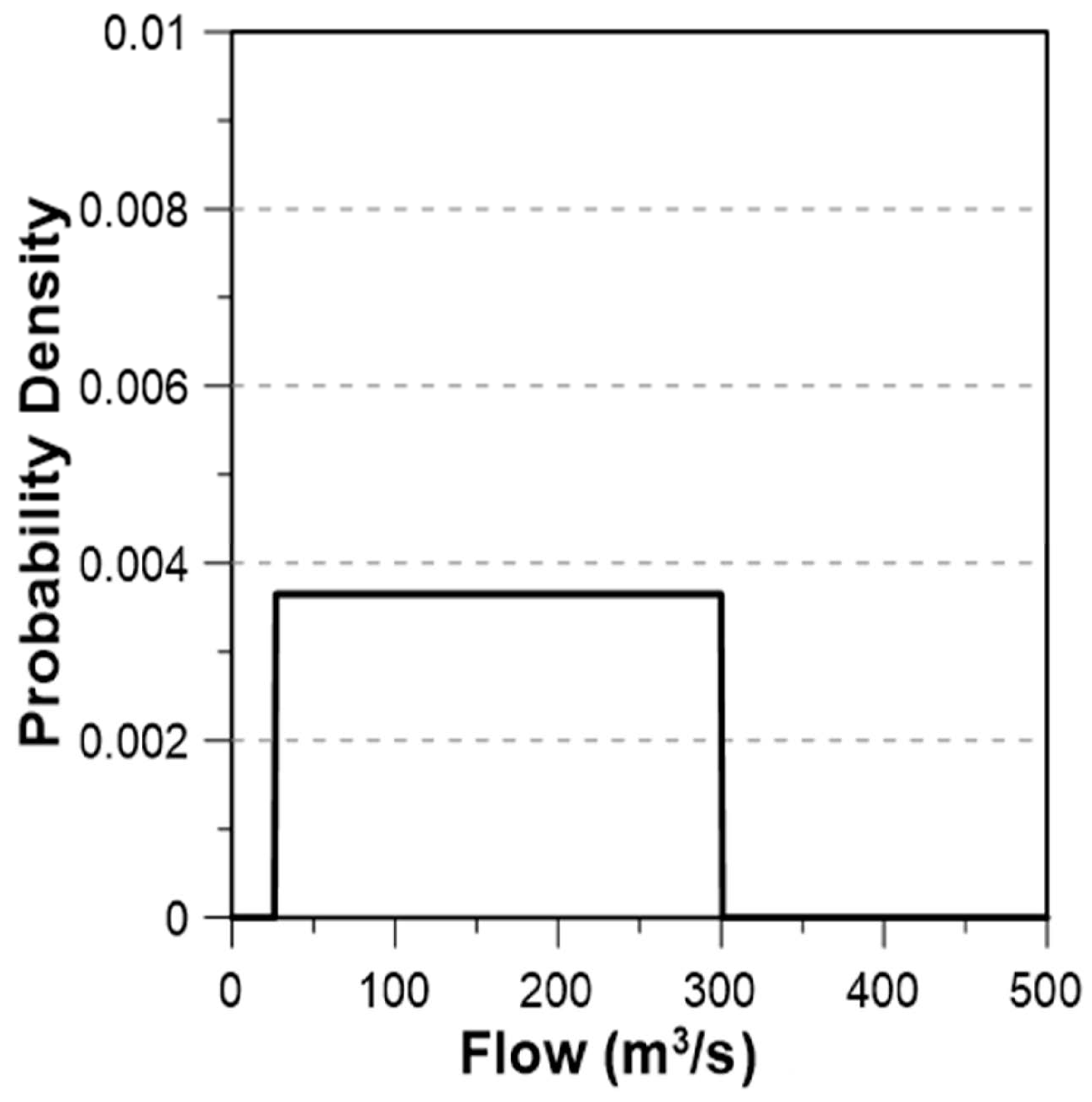
The prior distribution for the application of the Rigid ROM is determined individually for each inflow hydrograph, corresponding to each peak flow. In this study, the probability distribution of flow discharge prior to the implementation of the ROMs was derived from the SCS dimensionless unit hydrograph, which represents the inflow hydrograph based solely on peak flow. This method assumes a linear variation along both the rising and recession limbs of the hydrograph (Figure S2), resulting in a uniformly distributed probability of discharge values over the hydrograph’s duration, as shown in Figure 2. Thus, a uniform prior distribution was assumed, ranging from the minimum peak flow to the specified peak flow. Note that the minimum peak flow is set to be 20 m3/s in this study, referring to the observed values at the study area, which efficiently excludes low flows. This uniform distribution is consistently applied both before and after the peak flow. Such an assumption is reasonable, as the inflow increases linearly up to the peak flow and decreases similarly afterward, ensuring equal probability for all flow rates within the range. By considering an effectively infinite number of inflow hydrographs, this assumption accommodates various exceptions. Figure 2 illustrates the prior distribution for a peak flow of 300 m3/s as an example, demonstrating its symmetry before and after the peak flow, as previously stated.
(4)
Combination of the priori distributions and likelihood functions.
The posterior distribution is derived by applying the likelihood function to the prior distribution. Before the peak flow, when the constant rate ROM is applied, the Kronecker delta function is employed as the likelihood function (Equations (4) and (5)). In this context, α is assumed to be 0.5, consistent with the value adopted by the Andong Dam [22]. This parameter is also used in Section 4. After the peak flow, the constant magnitude ROM is applied, and the likelihood function becomes a combination of the uniform function and the Dirac delta function (Equations (6) and (7)). The constant magnitude, as previously explained, is defined as the product of the peak flow and the constant rate. A detailed application procedure of the likelihood function to the probability distribution of the inflow data is described in the Supplementary Materials (Text S1).
(5)
Derivation of the posteriori distribution for each peak flow.
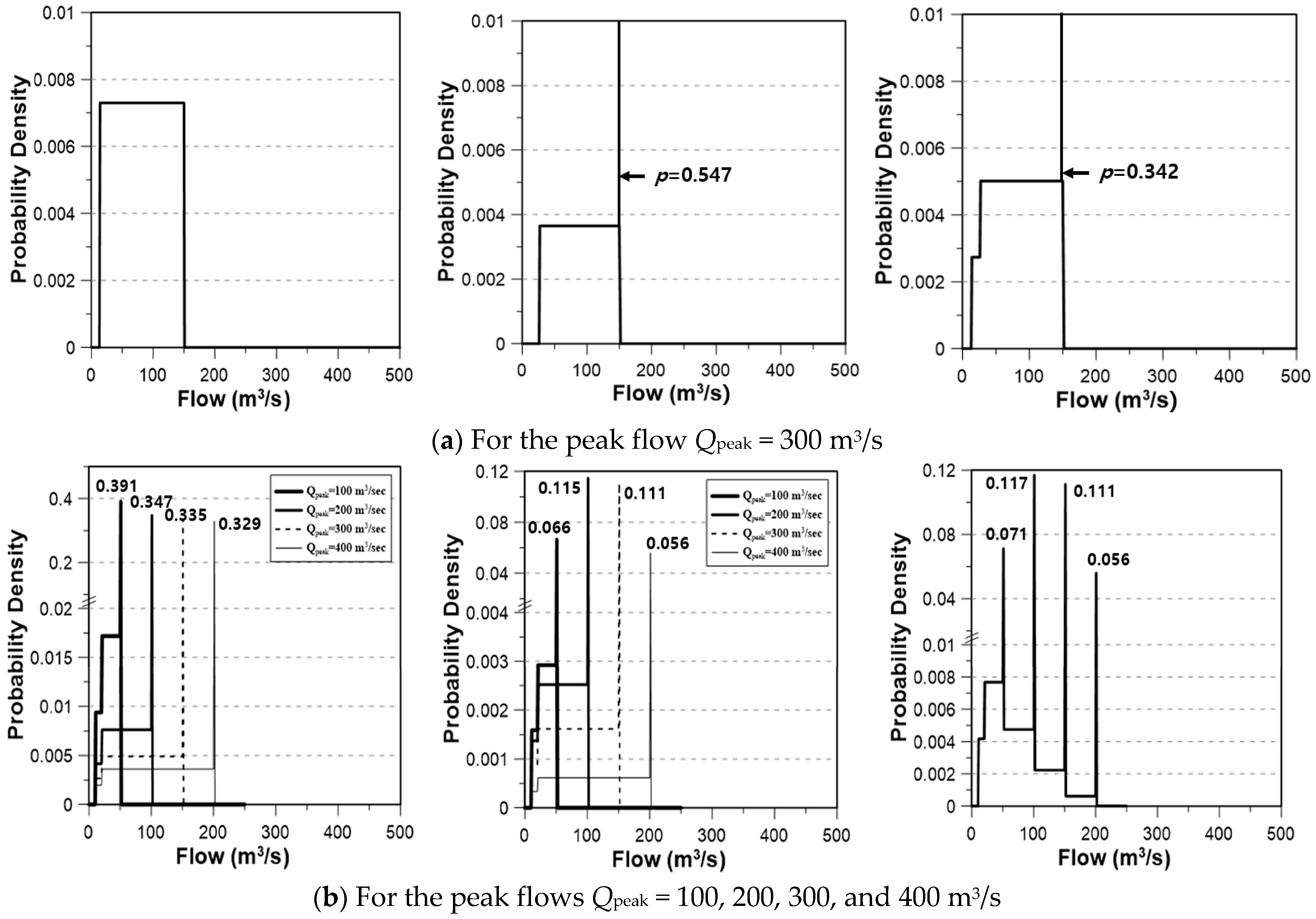
Figure 3a illustrates the posterior distribution for a peak flow of 300 m3/s. The first panel shows the posterior distribution before the peak flow, where the probability is uniform between 10 and 150 m3/s and zero beyond 150 m3/s. This outcome aligns with the prior distribution assumptions: a peak flow of 300 m3/s and a constant rate of 0.5. Additionally, with a minimum peak flow of 20 m3/s, the smallest outflow is derived as 10 m3/s, resulting in a uniform probability of 0.0073—twice the value of the prior distribution.
The second panel of Figure 3a depicts the posterior distribution after the peak flow. With a constant magnitude of 150 m3/s, the probability distribution between 20 and 150 m3/s remains uniform, mirroring the prior distribution. However, the probability for the outflow at 150 m3/s increases to 0.547, reflecting the influence of the Dirac delta function. The final panel presents the weighted sum of the posterior distributions before and after the peak flow, with weights determined by the inflow volume ratios of 0.374 and 0.626, respectively. These ratios correspond to the base time before and after the peak flow, following the SCS dimensionless unit hydrograph concept (1:1.67) (Figure S2). Specifically, the weight assigned to the posterior distribution before the peak flow is calculated as 1/(1 + 1.67) = 0.374, while the weight after the peak flow is 1/(1 + 1.67) = 0.626. This weighting approach was adopted to reflect the relative influence of each segment (i.e., before and after the peak flow) in deriving the overall posterior distribution for the triangular hydrograph (Figure S2). Given that the SCS dimensionless unit hydrograph assumes linear rising and recession limbs, it is justifiable to assume that the occurrence probability of flow discharge is linearly proportional to the base time, thereby supporting this weighting scheme. Consequently, the probabilities for specific ranges are determined as follows: 0–10 m3/s (0.000), 10–20 m3/s (0.0027), 20–150 m3/s (0.0049), and 150 m3/s (0.342).
(6)
Probability distribution of the outflow.
The probability distribution of the outflow simply becomes the weighted sum of all the derived posterior distributions, as shown in the last panel of Figure 3a. Here, the weights were determined by considering the probability density of the peak flow. As an example, in this part of the study, four different peak flows were considered, that is, 100, 200, 300, and 400 m3/s. Based on Figure S3, their occurrence probabilities were assigned as 0.17, 0.33, 0.33, and 0.17, respectively. The first panel of Figure 3b shows the posterior distributions derived for each peak flow case, the second panel of Figure 3b shows the same, but multiplied by their weights; and finally, the last panel of Figure 3b shows their sum. The last panel of Figure 3b shows that the probability density increases rapidly up to the outflow 20 m3/s, and then, as the outflow increases, it decreases rather slowly. Four peaks can also be found, which are simply the results of applying the constant magnitude ROM. If considering more peak flows, these abrupt peaks will disappear due to smoothing.
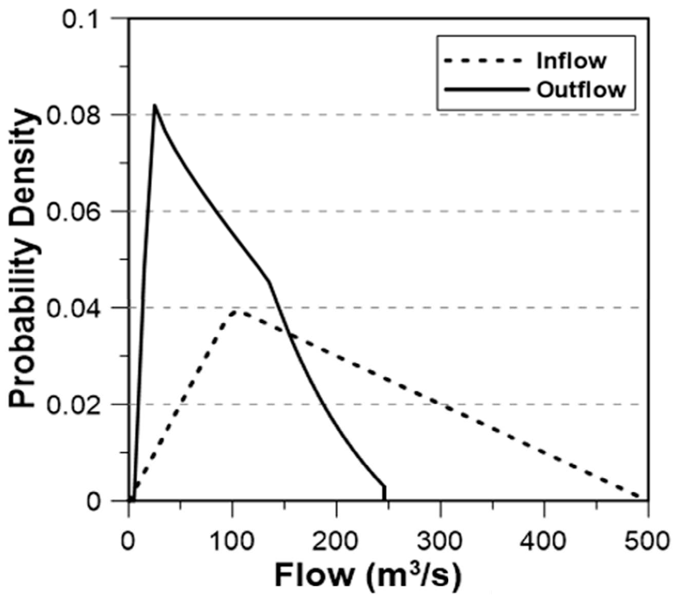
In this part of the study, all the peak flows were considered to derive the probability distribution of the outflow for the given peak flow in Figure S3. To numerically derive the result, the peak flows were considered discretely by introducing the interval x = 10 m3/s from the minimum peak flow 10 m3/s to the maximum 500 m3/s. In Figure 4, the dotted line represents the probability distribution of the inflow, while the solid line represents that of the outflow. This figure indicates that the probability of outflow between 0 and 10 m3/s is zero, a result of the predefined minimum peak flow. The probability density sharply increases from 10 m3/s, reaching a mode at 30 m3/s with a probability of 0.082, and then gradually decreases, reaching zero at 250 m3/s. The slope of the distribution changes noticeably after the mode, reflecting the influence of the peak inflow distribution, which peaks at 250 m3/s. Beyond this threshold, the probability of outflows exceeding 250 m3/s becomes negligible.

3. Study Area and Data

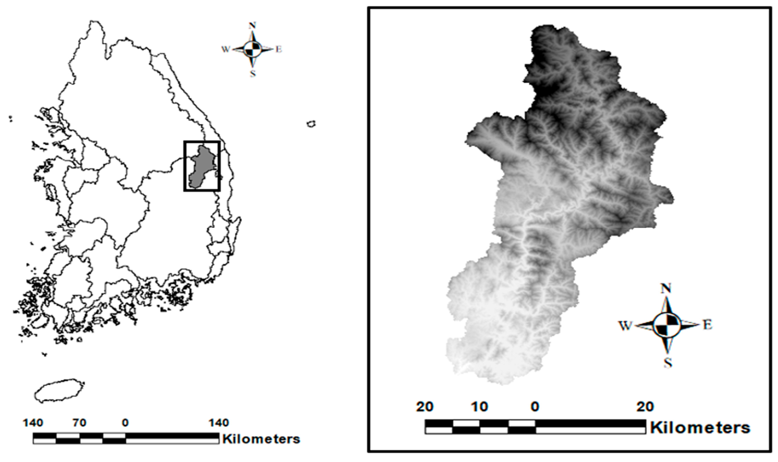
In this study, Andong Dam is presented as a case example. The dam is situated in the Nakdong River Basin, which encompasses the southern region of the Republic of Korea. Specifically, Andong Dam is located along the main stream of the Nakdong River. The area of the Andong Dam Basin is 1584 km2, the average elevation is 550 m, and the channel length is 171 km. Andong Dam is a rockfill dam 83 m in height and 612 m in length, with a 1248 million m3 storage capacity and 91,599 kW power generation capacity. Andong Dam controls the flood volume of 110 million m3 per year and supplies 926 million m3 for domestic, agricultural, and industrial purposes. It has been proven effective for both flood control and conservation [49]. Figure 5 illustrates the location and digital elevation map of the Andong Dam Basin.
The Bayesian method was applied to the inflow data of Andong Dam, specifically, the runoff data at the outlet of the Andong Dam Basin. This study utilized hourly inflow data recorded from 2010 to 2019, which were obtained from the K-water open data portal (http://opendata.kwater.or.kr/ accessed on 16 August 2024). Figure S4 presents the time series of the 10-year inflow dataset employed in the analysis. Notably, the maximum hourly inflow of 14,408 m3/s was recorded on 23 June 2012. In the design of the Andong Dam, the Rigid ROM was applied with a constant rate of 0.5. Additionally, based on the analysis of the observed peak time Tpeak and peak flow Qpeak, a linear relation between them could be assumed. For example, for the peak flow Qpeak = 500 m3/s, the peak time Tpeak was determined to be 5 h, and for Qpeak = 1000 m3/s, it was 10 h.

4. Results and Discussion

4.1. Verification of the Bayesian Replacement for the ROMs

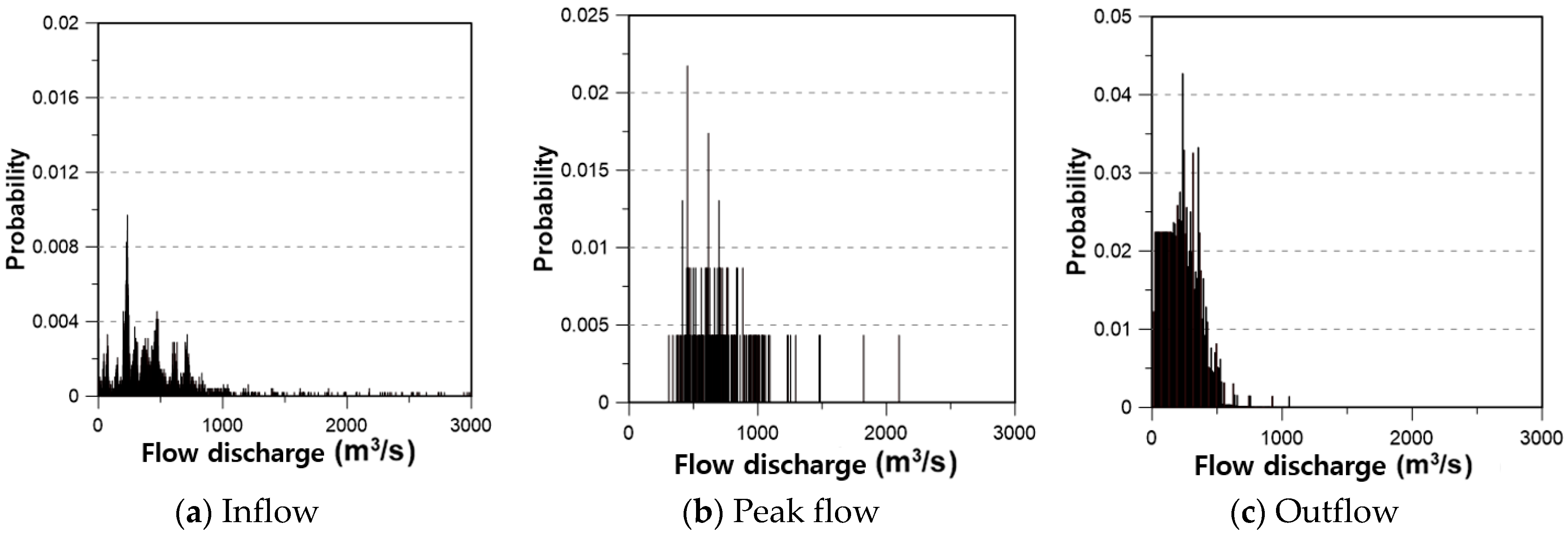
In this part of the study, the Bayesian method was applied to the inflow data in the year 2019, whose result was then analyzed to verify the use of the Bayesian method for the Rigid ROM. The prior distribution was derived by analyzing the observed inflow data from the Andong Dam in 2019 (Figure 6a). The mean of the inflow data was estimated to be 366 m3/s, and the mode was found to be 234 m3/s with a probability of 0.009, as can be seen in Figure 6a. More than 40% of the inflow was concentrated in the range from 200 to 400 m3/s, and the probability of even higher inflow was found to be rather low.
The application of the Rigid ROM to the observed inflow data at Andong Dam follows the procedure outlined in Section 2.3. First, the peak flow distribution was derived by analyzing observed inflow data, defining peak flow as the highest flow rate during events where direct runoff lasted at least three hours. Given the dam’s concentration time of approximately 13 h [50], runoff lasting one or two hours was considered to be a minor fluctuation. Figure 6b illustrates the peak flow distribution, with a mean peak flow of 768 m3/s—substantially higher than the overall mean inflow of 366 m3/s. The minimum peak flow was identified as 24 m3/s, representing the average dam release for hydro-power generation in 2019. For posterior distribution calculations, an interval of ∆x = 10 m3/s was used. Figure 6c shows the outflow distribution derived from the Rigid ROM, with the highest probability observed in the 230–240 m3/s range (probability = 0.043).
The results were compared with those obtained through ROM simulation to validate the application of the Bayesian method. Figure 7 presents histograms of outflow data simulated using the ROM simulation and Bayesian method based on 2019 inflow data. The probabilities of outflows ranging from 0 to 200 m3/s were 0.449 and 0.421 for the ROM simulation and Bayesian method, respectively, while the probabilities for the 200–400 m3/s range were 0.451 and 0.465, respectively. The histograms indicate a high degree of similarity, though some differences exist. These differences, albeit minor, are attributed to the use of a simplified representative inflow hydrograph, which assumes uniformity despite the potential for significant variations, even with the same peak flow. Additionally, complex multi-peak events were excluded from the analysis. These limitations introduce uncertainty into the results; however, the comparison demonstrates that the Bayesian method effectively reproduces the ROM simulation outcomes with high precision. This validates the methodology and likelihood function developed in this study.

4.2. Effect of the Dam Operation on the Downstream Flow–Duration

For the planning of a new dam, the operational effects are typically assessed through simulation studies. In this study, dam inflow data were derived from observed rainfall data using rainfall runoff analysis. However, when rainfall data are unavailable, alternative methods must be employed. Notably, this research did not involve rainfall data generation or rainfall runoff analysis; instead, it utilized existing inflow data collected over a 10-year period from 2010 to 2019.
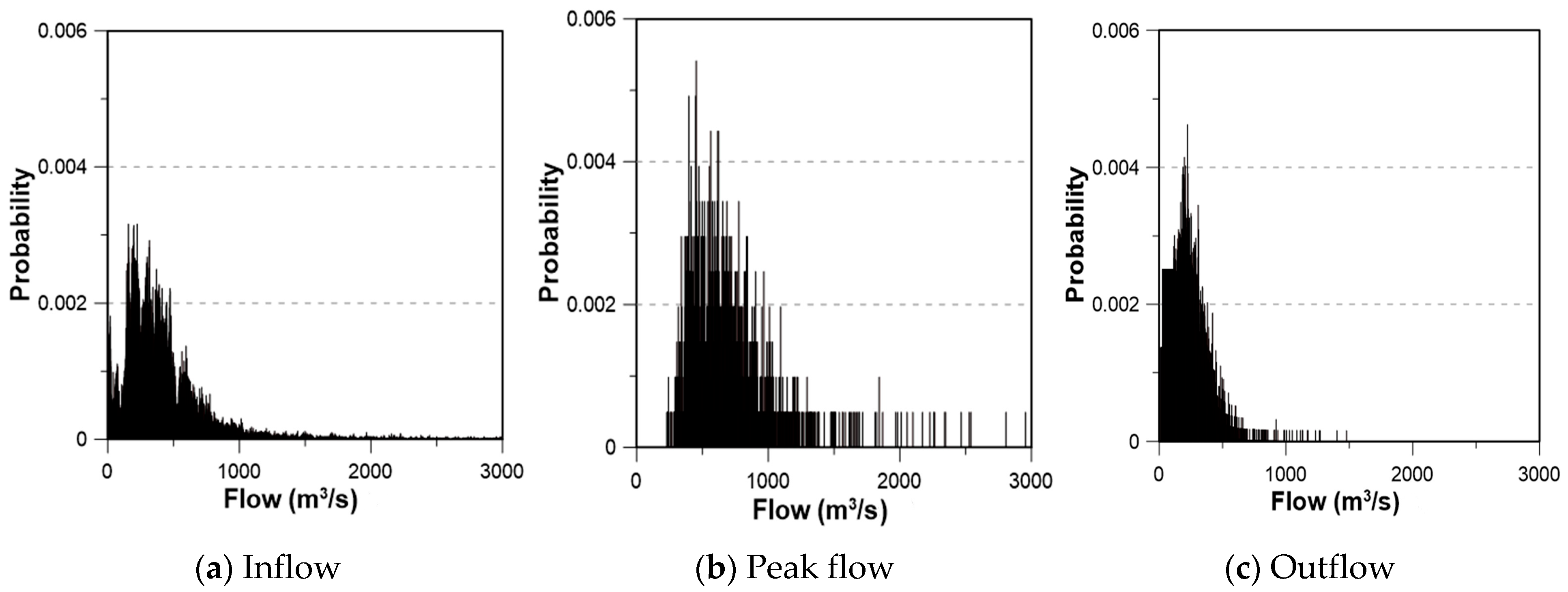
First, Figure 8a gives the probability distribution of the inflow data. The mode was found at the inflow of 223 m3/s. Figure 8b shows the derived probability distribution of the peak inflow. The mode was found at the inflow of 453 m3/s, with its probability of 0.0054. Compared with the probability distribution of the inflow data, the peak inflow data show higher probability at the high inflow values. This characteristic is also the same as in the data from 2019. Figure 8c gives the probability distribution of the outflow derived by applying the Bayesian method for the Rigid ROM. The mode was found at the range of 200–210 m3/s, with a probability of 0.0046. Most of the outflow was also found to be concentrated in the range from 0 to 400 m3/s, similar to the case of the year 2019. Compared with the probability distribution of the inflow data, the probability of outflow was more concentrated in the low-flow zone.
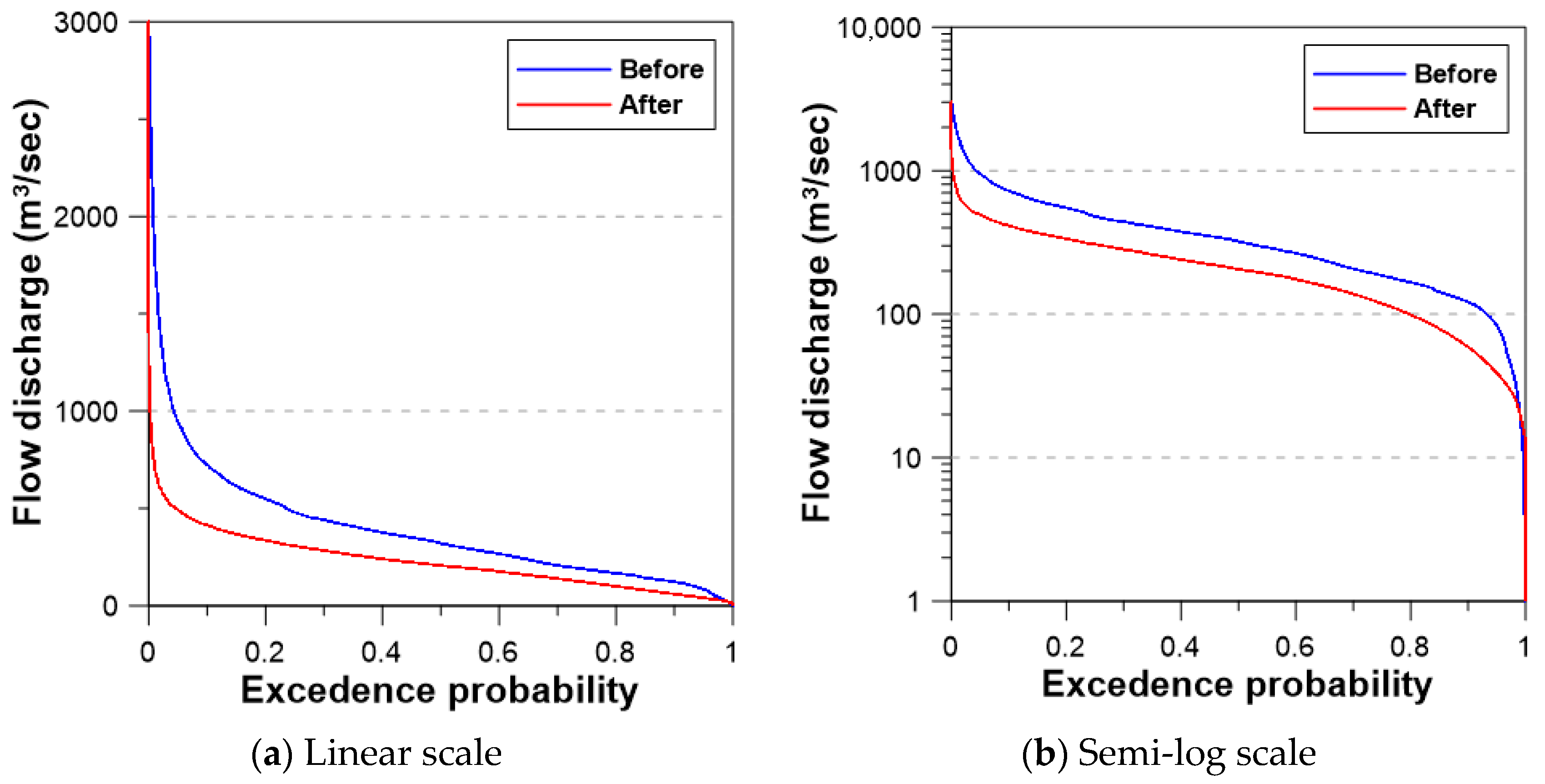
The comparison of flow–duration curves before and after dam construction (Figure 9) confirms the observed results. These curves represent cumulative probability distribution functions derived from the probability distributions shown in Figure 8a,c, with inflow data assumed to represent outflow data prior to dam construction. Notably, the flow–duration curve underwent significant changes following dam construction, characterized by an increased probability in the low-flow zone and a decreased probability in the high-flow zone. Consequently, both the mean and variance of flow were reduced, reflecting improvements in flow stability. This phenomenon, often referred to as flow–duration stabilization, describes the process by which the natural variability of river flows is diminished or regulated over time, leading to a more uniform flow regime downstream.
In fact, this result indicates several important notions. First, the risk of flooding has decreased. This must be one of the major objectives for building a dam. The number of outflows higher than 3100 m3/s (the design flood at the downstream part of the dam) has decreased from 27 to 14. That is, the dam construction has almost removed the risk of flooding. Second, the minimum flow (which is also called the drought flow or the 355-day flow) has increased by about 40% (from 25 to 35 m3/s). This result may be interpreted as the freshwater ecosystem being improved. However, this interpretation is somewhat controversial because the 95-day, 185-day, and 275-day flows have all decreased by about 40% (see Table 1). There are also many reports that frequent flooding is important to maintain the freshwater ecosystem [51,52].

4.3. Multiple Dams and Changes of Downstream Flow–Durations

The Bayesian method proposed in this study offers an effective approach for analyzing cascade reservoirs connected in series, leveraging the characteristics of Bayesian updates. As articulated by Puga et al. (2015) [53], the concept of “Today’s predictions are tomorrow’s priors” underpins the process of sequential updating, whereby the posterior distribution from one step of analysis (n in Equation (10)) is adopted as the prior information for the next step (n + 1 in Equation (10)). This iterative framework allows for the systematic incorporation of new information as it becomes available. The theoretical basis for this approach lies in Bayes’ theorem, which is fundamentally rooted in the multiplication rule—the law of total probability (Equation (10)). As illustrated in Figure S5, the inflow distribution at one reservoir is transformed into an outflow distribution, which subsequently serves as the inflow for the next reservoir. This iterative process can be repeated for as many reservoirs as necessary, enabling the straightforward derivation of flow characteristics at any location. By applying this method step by step, it is possible to comprehensively determine the flow distribution across the entire basin of interest.
P θ n + 1 ε = k L ε θ n + 1 P θ n ε ,   n = 1,2 , 3 ,
The posterior distribution for a series connection was derived based on the concept of Bayesian updating, assuming all dams were identical to the Andong Dam. Using hourly inflow data from 2010 to 2019, a constant rate (α) of 0.5—applicable to the Andong Dam—was applied. Figure 10 illustrates the outflow distributions for the series connection, effectively reflecting the impact of reservoir operation. In this process, the outflow distribution of the first dam served as the inflow (prior) distribution for the second dam, whose outflow distribution was derived as the posterior by incorporating the likelihood function. This procedure was repeated to obtain the outflow distribution for the third dam. As shown in Figure 10, the mean and standard deviation of the outflow distribution decrease as the number of dams in the series increases.
The flow duration curves for this case of series connection can be found in Figure S6. These flow–duration curves are simply the cumulative probability distribution functions of those probability distributions in Figure 10. As the number of dams increases, the probability of low flow increases and that of high flow decreases. More than 90% of the inflow data were concentrated in the range from 100 m3/s to 1000 m3/s. However, after passing through three dams, most of the flow becomes concentrated in the range from 20 m3/s to 100 m3/s. The probability of peak flow over 3100 m3/s (i.e., the design flood at the downstream part of the dam) also significantly decreased as the number of dams increased from 0.59% in the inflow distribution, 0.31% after the first dam, 0.11% after the second dam, and 0.10% after the third dam.

4.4. Implications and Limitations

The Bayesian method shows promise as an alternative to the ROM, provided that an appropriate likelihood function reflecting the ROM’s release rules is established. This approach enables the derivation of outflow probability distributions, facilitating assessments of the Rigid ROM and the impact of dams on downstream runoff. We also confirmed that the Bayesian method was also valid for other dams with different constant rates from 0.3 to 0.54 (Figure S7). If the constant rate decreases, the posterior PDF is expected to exhibit a peak probability at lower flow values. Conversely, as the constant rate increases, the PDF shifts in the opposite manner, indicating higher peak probabilities at larger flow values. The proposed Bayesian framework is also applicable to inflow data generated through hydrological modeling driven by General Circulation Model (GCM) inputs, which is particularly advantageous for data-sparse regions. This enables the projection of future flow–duration characteristics under continued reservoir operations in the coming decades. However, such applications necessitate robust and well-calibrated hydrological modeling to ensure reliability. Its applicability extends to complex scenarios, including multi-reservoir systems, dam construction or removal, and operational method changes. By iteratively updating posterior distributions—where the posterior of one reservoir becomes the prior for the next—and employing general likelihood functions for the ROM, this method offers a simplified, simulation-free framework for addressing diverse water resource management challenges.
The homogenization of flow–duration regimes caused by dam operations may offer benefits such as more stable baseflows and reduced flood risk; however, it also poses significant ecological drawbacks, particularly when combined with drought conditions, by simplifying ecosystem networks [54,55,56]. For instance, Poff et al. (2007) [57] analyzed 186 long-term streamflow records across the continental United States and found that dams primarily altered the magnitude and timing of ecologically critical high and low flows, resulting in flow regime homogenization. This hydrological alteration fosters biological homogenization of freshwater fish assemblages, diminishes ecological resilience, and reduces regional uniqueness—thereby weakening landscape-scale resilience to global change. Furthermore, Stein et al. (2021) [58] proposed the California Environmental Flows Framework, grounded in the principle that natural flow variability is essential to sustaining freshwater biodiversity. Collectively, these studies underscore the ecological necessity of maintaining a certain degree of natural flow variability to support ecosystem health.
In the Republic of Korea, dam operations during the flood season are subject to various sources of uncertainty. Notably, operator subjectivity can substantially influence decision-making, as adjustments to ROMs are often made in response to forecasted precipitation and the flood conditions both upstream and downstream. Consequently, the observed outflows from a dam during flood events may not fully represent the application of a specific ROM, such as the Rigid ROM adopted in this study. Despite this, the current analysis assumes that all discharges during the flood season are governed exclusively by the Rigid ROM. To address this discrepancy, simulated data were utilized as the reference for evaluating model performance, rather than observed records.
The results of this study may be sensitive to the definition, assumptions, or parameter settings. Specifically, while the continuous form of Bayes’ theorem employs probability density functions and integrates over the total probability space, the discrete implementation relies on probability mass functions and numerical summation. As such, the resulting posterior distribution may vary depending on the size of the unit interval (Δθ) used in the discretization. Nevertheless, this discrepancy becomes negligible when Δθ is sufficiently small. Therefore, if Δθ is chosen such that the deviation between the continuous and discrete formulations falls within an acceptable margin of error, the discrete approximation can be regarded as both valid and reliable, which was demonstrated in this study.
Second, while this study employs the SCS dimensionless unit hydrograph—which assumes linear rising and recession limbs—it is acknowledged that this simplification does not fully reflect the complexity of real-world hydrograph behavior. Moreover, this approach introduces uncertainty into the assumption of a uniform prior distribution. Given the impracticality of accounting for the infinite variability in hydrograph shapes arising from diverse rainfall events, a representative hydrograph was required. We thus selected one derived solely from peak flow information, consistent with the focus of our study, wherein the Rigid ROM primarily governs peak inflow conditions during flood events. This necessitated the assumption that peak flow does not occur in multiple successive stages—a known limitation of the current approach. Nevertheless, the SCS dimensionless unit hydrograph provides a broadly accepted and computationally efficient approximation of the temporal distribution of runoff. Its widespread use in contemporary hydrologic design studies further supports its suitability [59,60,61]. Future research may explore the sensitivity of simulation outputs to the choice of hydrograph shape by directly comparing outcomes derived from the observed hydrographs and synthetic counterparts.

5. Summary and Conclusions

This study introduces a Bayesian approach as an alternative to the traditional ROM for detecting changes in downstream flow–duration more effectively. By integrating the inflow data’s PDF with a likelihood function associated with the ROM, the downstream runoff’s PDF is derived. The focus is on the Rigid ROM, commonly used in the Republic of Korea, which includes the constant rate and constant magnitude ROMs. A critical contribution of this research is the derivation of the likelihood function for Rigid ROM. Using inflow data from the Andong Dam in the Republic of Korea during 2019, the proposed Bayesian method was applied to estimate the downstream runoff’s PDF, which was validated against simulation results. This study also analyzed changes in downstream flow–duration following dam construction based on data from 2010 to 2019. Furthermore, the method’s adaptability was demonstrated by extending its application to multi-dam scenarios through Bayesian updating.
This study derived the likelihood function for the Rigid ROM by incorporating its release rules, which were expressed using mathematical functions: the Kronecker delta for constant rate ROM and a combination of uniform and Dirac delta functions for constant magnitude ROM. The release rule of the Rigid ROM transitions from a constant rate before the inflow peak to a constant magnitude after the peak, necessitating prior information on peak inflow distribution and representative hydrographs. The posterior distribution was calculated by applying the likelihood function to prior distributions, assuming a triangular hydrograph as the inflow probability distribution. Uniform prior distributions were separately applied for pre- and post-peak inflows, resulting in segmented posterior distributions that were combined to determine the overall posterior distribution. By repeating this procedure across peak flows, the outflow probability distribution was derived and validated through simulation, revealing minor deviations due to simplified inflow assumptions. An analysis of the flow–duration curve indicated that the Rigid ROM increased low-flow probabilities while reducing the likelihood of higher outflows.

Supplementary Materials

The following supporting information can be downloaded at: https://www.mdpi.com/article/10.3390/w17142078/s1, Figure S1: Likelihood functions of the constant rate ROM (a) and the constant magnitude ROM (b) for given inputs and parameters. Inflow x and constant rate α are set to be 500 m3/s and 0.5, respectively, for constant rate ROM case. The constant magnitude Q0 is 300 m3/s; Figure S2: Inflow hydrographs assumed for the given peak flows (Qpeak = 100, 300, and 500 m3/s). In this example, the peak times were also assumed to be 1, 3, and 5 hours, respectively. Based on Equation (9), the base time becomes 2.67, 8.01, and 13.35 hours, respectively; Figure S3: Assumed probability distribution of the peak flow. The range of the peak flow is from 0 to 500 m3/s, and the mode lies on 250 m3/s, with its probability density of 0.004; Figure S4: Time series plots of areal average rainfall and inflow data of the Andong Dam during the 10 year period from 2010 to 2019; Figure S5: Application schematic of deriving the posterior distribution for the case of series connection based on the concept of Bayesian update; Figure S6: Comparison of flow-duration curves for the case of series connection with different scales; Figure S7: Comparison of histograms for the Bayesian application and ROM simulation with different constant rates. The methods are applied to two different periods (a) Year of 2019 and (b) Years of 2010-2019; Text S1: Sample applications of the likelihood functions for the constant rate and constant magnitude ROMs.

Author Contributions

Conceptualization, C.Y. and W.N.; methodology, C.Y.; validation, W.N.; formal analysis, W.N.; investigation, C.Y.; writing—original draft preparation, W.N.; writing—review and editing, C.Y.; visualization, W.N. All authors have read and agreed to the published version of the manuscript.

Funding

This work was supported by the National Research Foundation of Korea (NRF) grant funded by the Korea government (MSIT) (No. RS-2021-NR060085).

Data Availability Statement

The inflow data of Andong Dam used during the study are available from the K-Water website (https://opendata.kwater.or.kr accessed on 16 August 2024). The following data, models, or code that support the findings of this study are available from the corresponding author upon reasonable request.

Conflicts of Interest

The authors declare no conflicts of interest.

References

  1. Choi, S.U.; Yoon, B.; Woo, H. Effects of dam-induced flow regime change on downstream river morphology and vegetation cover in the Hwang River, Korea. River Res. Appl. 2005, 21, 315–325. [Google Scholar] [CrossRef]
  2. Wang, Y.; Rhoads, B.L.; Wang, D. Assessment of the flow regime alterations in the middle reach of the Yangtze River associated with dam construction: Potential ecological implications. Hydrol. Process. 2016, 30, 3949–3966. [Google Scholar] [CrossRef]
  3. Magilligan, F.J.; Nislow, K.H. Changes in hydrologic regime by dams. Geomorphology 2005, 71, 61–78. [Google Scholar] [CrossRef]
  4. Mineda, H.; Nukazawa, K.; Suzuki, Y. Assessing environmental flow alterations induced by dams and climate change using a distributed hydrological model at catchment scale. J. Water Clim. Change 2023, 14, 4821–4836. [Google Scholar] [CrossRef]
  5. Karimidastenaei, Z.; Darabi, H.; Torabi Haghighi, A. Impact of dam construction on suspended sediment load alteration. In Proceedings of the EGU General Assembly Conference Abstracts, Vienna, Austria, 14–19 April 2024; p. 5559. [Google Scholar]
  6. Bussi, G.; Darby, S.E.; Whitehead, P.G.; Jin, L.; Dadson, S.J.; Voepel, H.E.; Vasilopoulos, G.; Hackney, C.R.; Hutton, C.; Berchoux, T.; et al. Impact of dams and climate change on suspended sediment flux to the Mekong delta. Sci. Total Environ. 2021, 755, 142468. [Google Scholar] [CrossRef]
  7. Yoon, Y.N.; Kang, B.S.; Kim, U.T.; Kim, J.H.; Ko, I.H. An analysis on the variation of long-term runoff characteristics of basin before and after dam construction II. An analysis on the variation of long-term runoff characteristics of basin using model parameters estimation. J. Korean Soc. Civ. Eng. 1998, 18, 461–468. [Google Scholar]
  8. Yoo, C.; Kim, J.K.; Kim, J.H.; Yoon, Y.N. Change of hydrometeorologic environment due to dam construction: 1. Estimation of changing point. J. Korean Soc. Civ. Eng. 2003, 23, 87–94. [Google Scholar]
  9. Yoo, C.; Kim, K.; Yoon, Y. Change of hydrometeorologic environment due to dam construction: 2. Change of means. J. Korean Soc. Civ. Eng. 2003, 23, 95–103. [Google Scholar]
  10. Choi, S.; Yoon, B.; Woo, H.; Cho, K.H. Effect of flow-regime change due to damming on the river morphology and vegetation cover in the downstream river reach: A case of Hapchon dam on the Hwang river. J. Korea Water Resour. Assoc. 2004, 37, 55–66. [Google Scholar] [CrossRef]
  11. Ahn, J.H.; Yoo, C.; Kim, H.Y.; Yoon, Y.N. An assessment on the geographical boundary of hydrometeorologic changes due to dam construction. J. Korea Water Resour. Assoc. 2005, 38, 293–300. [Google Scholar] [CrossRef]
  12. Poff, N.L.; Allan, J.D.; Bain, M.B.; Karr, J.R.; Prestegaard, K.L.; Ricther, B.D.; Sparks, R.E.; Stromverg, J.C. The natural flow regime: A paradigm for river conservation and restoration. Bioscience 1997, 47, 769–784. [Google Scholar] [CrossRef]
  13. Chen, Y.D.; Yang, T.; Xu, C.Y. Hydrologic alteration along the Middle and Upper East River (Dongjiang) basin, South China: A visually enhanced mining on the results of RVA method. Stoch. Environ. Res. Risk Assess. 2010, 24, 9–18. [Google Scholar] [CrossRef]
  14. Yang, Z.; Yan, Y.; Liu, Q. Assessment of the flow regime alterations in the Lower Yellow River, China. Ecol. Inform. 2012, 10, 56–64. [Google Scholar] [CrossRef]
  15. Rood, S.B.; Samuelson, G.M.; Braatne, J.H.; Gourley, C.R.; Hughes, F.M.R.; Mahoney, J.M. Managing river flows to restore floodplain forests. Front. Ecol. Environ. 2005, 3, 193–201. [Google Scholar] [CrossRef]
  16. Burke, M.; Jorde, K.; Buffington, J.M. Application of a hierarchical framework for assessing environmental impacts of dam operation: Changes in streamflow, bed mobility and recruitment of riparian trees in a western North American river. J. Environ. Manag. 2009, 90, S224–S236. [Google Scholar] [CrossRef]
  17. Mediero, L.; Garrote, L.; Martin-Carrasco, F. A probabilistic model to support reservoir operation decisions during flash floods. Hydrolog. Sci. J. 2007, 52, 523–537. [Google Scholar] [CrossRef]
  18. Zhang, Y.Y.; Xia, J.; Chen, J.F.; Zhang, M.H. Water quantity and quality optimization modeling of dams operation based on SWAT in Wenyu River catchment, China. Environ. Monit. Assess. 2011, 173, 409–430. [Google Scholar] [CrossRef]
  19. K-Water. Dam Operation Manual; K-Water: Daejeon, Republic of Korea, 2009. [Google Scholar]
  20. Lee, S.J. Development of Weather Forecast Correction Method and Application to Dam Operation. Master’s Thesis, Sejong University, Seoul, Republic of Korea, 2011. [Google Scholar]
  21. Huh, J.G. A Study on Operation of Reservoir Using Simulation Technique. Master’s Thesis, Soong-sil University, Seoul, Republic of Korea, 2016. [Google Scholar]
  22. K-Water. A Guidance for Practical Design of Hydraulic Structures: Dam (Investigation and Planning); K-Water: Daejeon, Republic of Korea, 2018. [Google Scholar]
  23. Yoo, C.; Shin, H.; Lee, J. Evaluation of the Storage Effect Considering Possible Redevelopment Options of the Peace Dam in South Korea. Water 2020, 12, 1674. [Google Scholar] [CrossRef]
  24. Karamouz, M.; Vasiliadis, H.V. Bayesian stochastic optimization of reservoir operation using uncertain forecasts. Water Resour. Res. 1992, 28, 1221–1232. [Google Scholar] [CrossRef]
  25. Kim, Y.O.; Palmer, R.N. Value of seasonal flow forecasts in Bayesian stochastic programming. J. Water Resour. Plan. Manag. 1997, 123, 327–335. [Google Scholar] [CrossRef]
  26. Kim, Y.O.; Eum, H.I.; Kim, S.U.; Lee, K.S. Monthly joint operations for the Nakdong multi-reservoir system in Korea. Water Int. 2007, 32, 416–427. [Google Scholar] [CrossRef]
  27. Liu, Y.; Qin, H.; Zhang, Z.; Yao, L.; Wang, Y.; Li, J.; Liu, G.; Zhou, J. Deriving reservoir operation rule based on Bayesian deep learning method considering multiple uncertainties. J. Hydrol. 2019, 579, 124207. [Google Scholar] [CrossRef]
  28. Ang, A.H.S.; Tang, W.H. Probability Concepts in Engineering Planning and Design; Wiley: New York, NY, USA, 1984. [Google Scholar]
  29. Bates, B.C.; Campbell, E.P. A Markov chain Monte Carlo scheme for parameter estimation and inference in conceptual rainfall-runoff modeling. Water Resour. Res. 2001, 37, 937–947. [Google Scholar] [CrossRef]
  30. Viglione, A.; Merz, R.; Salinas, J.L.; Blöschl, G. Flood frequency hydrology. Part III: A Bayesian analysis. Water Resour. Res. 2013, 49, 675–692. [Google Scholar] [CrossRef]
  31. Brandt, F.T.; Das, A.; Frenkel, J.; Taylor, J.C. Kronecker delta energy terms in thermal field theory. Phys. Rev. D 2002, 65, 085008. [Google Scholar] [CrossRef]
  32. Carbó-Dorca, R. Logical Kronecker delta deconstruction of the absolute value function and the treatment of absolute deviations. J. Math. Chem. 2011, 49, 619–624. [Google Scholar] [CrossRef]
  33. Koo, B.; Yoon, M.; Cho, S. Isogeometric shape design sensitivity analysis using transformed basis functions for Kronecker delta property. Comput. Method. Appl. Mech. Eng. 2013, 253, 505–516. [Google Scholar] [CrossRef]
  34. Liu, Y.; Gupta, H.V. Uncertainty in hydrologic modeling: Toward an integrated data assimilation framework. Water Resour. Res. 2007, 43, W07401. [Google Scholar] [CrossRef]
  35. Georgakakos, A.P.; Georgakakos, K.P.; Baltas, E.A. A state-space model for hydrologic river routing. Water Resour. Res. 1990, 26, 827–838. [Google Scholar]
  36. Namias, V. Application of the Dirac delta function to electric charge and multipole distributions. Am. J. Phys. 1977, 45, 624–630. [Google Scholar] [CrossRef]
  37. Prieto, F.; Lourenço, P.B.; Oliveira, C.S. Impulsive Dirac-delta forces in the rocking motion. Earthq. Eng. Struct. Dyn. 2004, 33, 839–857. [Google Scholar] [CrossRef]
  38. Engquist, B.; Tornberg, A.K.; Tsai, R. Discretization of Dirac delta functions in level set methods. J. Comput. Phys. 2005, 207, 28–51. [Google Scholar] [CrossRef]
  39. Eftekhari, S.A. A differential quadrature procedure with regularization of the Dirac-delta function for numerical solution of moving load problem. Lat. Am. J. Solids Struct. 2015, 12, 1241–1265. [Google Scholar] [CrossRef]
  40. Hjelmfelt, A.; Wang, M. General stochastic unit hydrograph. J. Irrig. Drain. Eng. 1994, 120, 138–148. [Google Scholar] [CrossRef]
  41. Monajemi, P.; Khaleghi, S.; Maleki, S. Derivation of instantaneous unit hydrographs using linear reservoir models. Hydrol. Res. 2021, 52, 339–355. [Google Scholar] [CrossRef]
  42. Lu, M.; Rogiers, B.; Beerten, K.; Gedeon, M.; Huysmans, M. Exploring river–aquifer interactions and hydrological system response using baseflow separation, impulse response modelling and time series analysis in three temperate lowland catchments. Hydrol. Earth Syst. Sci. 2022, 26, 3629–3649. [Google Scholar] [CrossRef]
  43. Bartlett, M.S.; Daly, E.; McDonnell, J.J.; Parolari, A.J.; Porporato, A. Stochastic rainfall-runoff model with explicit soil moisture dynamics. Proc. R. Soc. A Math. Phys. Eng. Sci. 2015, 471, 20150389. [Google Scholar] [CrossRef]
  44. Shin, Y.L.; Maeng, S.H.; Ko, I.H.; Lee, H.K. Development of reservoir operation model using simulation technique in flood season (I). J. Korea Water Resour. Assoc. 2000, 33, 745–755. [Google Scholar]
  45. Diskin, M.H.; Lane, L.J. Application of a Double Triangle Unit Hydrograph to a Small Semiarid Watershed; Arizona-Nevada Academy of Science: Glendale, AZ, USA, 1976. [Google Scholar]
  46. Kjeldsen, T.R. The Revitalised FSR/FEH Rainfall-Runoff Method; UK Centre for Ecology & Hydrology: Lancaster, UK, 2007. [Google Scholar]
  47. Luxon, N.; Christopher, M.; Pius, C. Validating the Soil Conservation Service triangular unit hydrograph (SCS-TUH) model in estimating runoff peak discharge of a catchment in Masvingo, Zimbabwe. Int. J. Water Res. Environ. Eng. 2013, 5, 157–162. [Google Scholar]
  48. SCS (Soil Conservation Service). National Engineering Handbook, Section 4: Hydrology; Soil Conservation Service: Washington, DC, USA, 1972.
  49. KNCOLD (Korea National Committee on Large Dams). The 40th Anniversary of the Korea National Committee on Large Dams: A History of Dam Design; Korea National Committee on Large Dams: Daejeon, Republic of Korea, 2012. [Google Scholar]
  50. Kim, H.T.; Shin, H. The development and application of GIS-based geomorpho-hydrological watershed model (G2WMS). J. Korean Soc. Hazard. Mitig. 2009, 9, 123–133. [Google Scholar]
  51. Molles, M.C., Jr.; Crawford, C.S.; Ellis, L.M.; Valett, H.M.; Dahm, C.N. Managed flooding for riparian ecosystem restoration: Managed flooding reorganizes riparian forest ecosystems along the middle Rio Grande in New Mexico. BioScience 1998, 48, 749–756. [Google Scholar] [CrossRef]
  52. Cross, W.F.; Baxter, C.V.; Donner, K.C.; Rosi-Marshall, E.J.; Kennedy, T.A.; Hall Jr, R.O.; Kelly, H.A.W.; Rogers, R.S. Ecosystem ecology meets adaptive management: Food web response to a controlled flood on the Colorado River, Glen Canyon. Ecol. Appl. 2011, 21, 2016–2033. [Google Scholar] [CrossRef] [PubMed]
  53. Puga, J.L.; Krzywinski, M.; Altman, N. Points of significance: Bayes’ theorem. Nat. Methods 2015, 12, 277–278. [Google Scholar] [CrossRef] [PubMed]
  54. Tonkin, J.D.; Merritt, D.M.; Olden, J.D.; Reynolds, L.V.; Lytle, D.A. Flow regime alteration degrades ecological networks in riparian ecosystems. Nat. Ecol. Evol. 2018, 2, 86–93. [Google Scholar] [CrossRef]
  55. Lu, X.; Gray, C.; Brown, L.E.; Ledger, M.E.; Milner, A.M.; Mondragón, R.J.; Woodward, G.; Ma, A. Drought rewires the cores of food webs. Nat. Clim. Chang. 2016, 6, 875–878. [Google Scholar] [CrossRef]
  56. Chalise, D.R.; Sankarasubramanian, A.; Ruhi, A. Dams and climate interact to alter river flow regimes across the United States. Earth’s Future 2021, 9, e2020EF001816. [Google Scholar] [CrossRef]
  57. Poff, N.L.; Olden, J.D.; Merritt, D.M.; Pepin, D.M. Homogenization of regional river dynamics by dams and global biodiversity implications. Proc. Natl. Acad. Sci. USA 2007, 104, 5732–5737. [Google Scholar] [CrossRef]
  58. Stein, E.D.; Zimmerman, J.; Yarnell, S.M.; Stanford, B.; Lane, B.; Taniguchi-Quan, K.T.; Obester, A.; Grantham, T.E.; Lusardi, R.A.; Sandoval-Solis, S. The California environmental flows framework: Meeting the challenges of developing a large-scale environmental flows program. Front. Environ. Sci. 2021, 9, 769943. [Google Scholar] [CrossRef]
  59. Shatnawi, A.; Ibrahim, M. Derivation of flood hydrographs using SCS synthetic unit hydrograph technique for Housha catchment area. Water Supply 2022, 22, 4888–4901. [Google Scholar] [CrossRef]
  60. Guo, J. General and analytic unit hydrograph and its applications. J. Hydrol. Eng. 2022, 27, 04021046. [Google Scholar] [CrossRef]
  61. dos Santos, C.I.; Carlotto, T.; Steiner, L.V.; Chaffe, P.L.B. Development of the Synthetic Unit Hydrograph Tool–SUnHyT. Appl. Comput. Geosci. 2023, 20, 100138. [Google Scholar] [CrossRef]
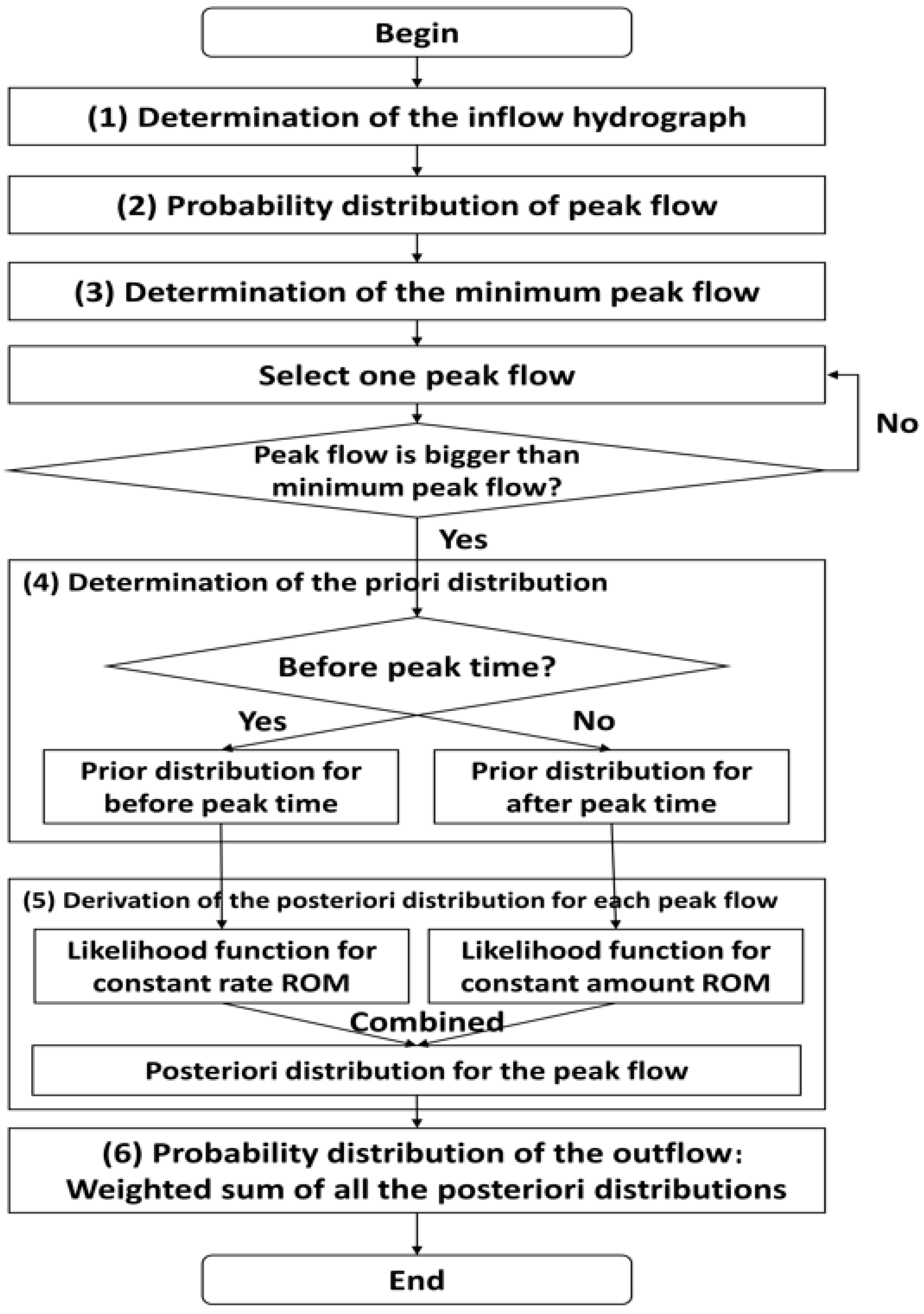
Figure 1. Application procedure of the Bayesian method in this study for the case of Rigid ROM.
Water 17 02078 g001
Figure 2. Prior distributions for the application of the Bayesian method for the Rigid ROM. In this example, the peak flow is set to 300 m3/s.
Water 17 02078 g002
Figure 3. Procedure for deriving the probability distribution of the outflow by applying the Bayesian method for the Rigid ROM. The application examples for one peak flow (a) and four different peak flows (b) are both shown. The left panel is the posterior distribution before the peak flow, the middle panel is the posterior distribution after the peak flow, and the right panel is their weighted sum.
Water 17 02078 g003
Figure 4. Comparison of probability distributions of inflow and outflow derived by applying the Bayesian method for the Rigid ROM as a sample case provided by Figure 2 and Figure S3.
Water 17 02078 g004
Figure 5. Location of the Andong Dam and its basin along with the digital elevation map.
Water 17 02078 g005
Figure 6. Probability distribution of the inflow data (i.e., prior distribution) (a), the peak flow (b), and the posterior distribution (i.e., probability distribution of the outflow data for the year 2019) derived by applying the Bayesian method for the Rigid ROM (c).
Water 17 02078 g006
Figure 7. Comparison between the ROM simulation results (a) and the outcomes obtained through the application of the Bayesian method (b) for the Rigid ROM (year 2019).
Water 17 02078 g007
Figure 8. Probability distributions of the inflow (a), peak flow (b), and outflow (c) derived by applying the Bayesian method for the Rigid ROM (from 2010 to 2019).
Water 17 02078 g008
Figure 9. Comparison of flow–duration curves before and after dam construction with different scales.
Water 17 02078 g009
Figure 10. Probability distributions of the inflow and outflow distributions for the case of series connection derived through Bayesian updates for Rigid ROM. Outflow (first, second, third dam) represents the discharges from each dam in the series, with the outflow from the first dam becoming the inflow for the second, and so on.
Water 17 02078 g010
Table 1. Change of annual flow–durations before and after dam construction.
95-Day Flow (m3/s)185-Day Flow
(m3/s)
275-Day Flow (m3/s)355-Day Flow (m3/s)Coefficient of Flow–Duration
Before4953352052568
After3052051153519
Change (%)−38−39−4440−72
Disclaimer/Publisher’s Note: The statements, opinions and data contained in all publications are solely those of the individual author(s) and contributor(s) and not of MDPI and/or the editor(s). MDPI and/or the editor(s) disclaim responsibility for any injury to people or property resulting from any ideas, methods, instructions or products referred to in the content.