GIS-Based Spatial Autocorrelation and Multivariate Statistics for Understanding Groundwater Uranium Contamination and Associated Health Risk in Semiarid Region of Punjab, India

Abstract

To provide safe drinking water in contaminated hydrogeological environments, it is essential to have precise geochemical information on contamination hotspots. In this study, Geographic Information System (GIS) and multivariate statistics were utilized to analyze the spatial patterns, occurrence, and major factors controlling uranium (U) concentrations in groundwater. The global and local Moran’s I indices were utilized to detect hotspots and cool spots of U distribution. The substantial positive global Moran’s I index (at a p-value of 0.05) revealed a geographical pattern in U occurrences. The spatial clusters displayed patterns of drinking water source with U concentrations below and above the WHO limit, categorized as “regional U cool spots” and “regional U hotspots”, respectively. Spatial autocorrelation plots revealed that the high–high potential spatial patterns for U were situated in the northeastern region of the study area. As the order of queen’s contiguity increased, prospective low–high spatial patterns transitioned from the Faridkot district to the Muktsar district for U. Further, the multivariate statistical analysis methods such as correlation and principal component analysis (PCA) plots revealed substantial positive associations (p-value < 0.05) between U and total dissolved solids (TDS), salinity (SL), bicarbonate (HCO₃⁻), and sodium (Na) in groundwater from both shallow and deeper depth, indicating that these water quality parameters can significantly influence the occurrence of U in the groundwater. The output of the random forest model shows that among the groundwater parameters, TDS is the most influential variable for enrichment of U in groundwater, followed by HCO₃⁻, Na, F⁻, SO₄²⁻, Mg, Cl⁻, pH, NO₃⁻, and K concentrations. Additionally, the results of health risk assessment indicate that 47.86% and 41.3% of samples pose risks to children and adults, respectively, due to F⁻−contamination. About 93.49% and 89.14% of samples pose a risk to children and adults, respectively, due to U contamination, whereas 51.08% and 39.13% of samples pose a risk to children and adults, respectively, from NO₃⁻ contamination. The current data indicates an urgent need to create cost-effective and efficient remediation techniques for groundwater contamination in this region.

1. Introduction

Groundwater, a convenient source of water, occurs in underground natural reservoirs [1,2]. It is an essential resource for sustaining life and promoting global economic growth [3]. Groundwater is the only source of fresh water for billions of people in the world and is utilized for industrial, agricultural, domestic, and food production purposes [4,5]. In arid and semiarid regions where rainfall is less, the groundwater is an essential water source for daily use [6,7,8]. As a result, the quality and quantity of groundwater have significantly deteriorated worldwide due to overexploitation, excess use of insecticides and pesticides, rapid urbanization, and large-scale industrialization [9]. Because groundwater directly impacts human health and ecosystem sustainability, understanding its quality is crucial for evaluating its potential uses [10,11,12,13]. Poor groundwater quality has been reported in many parts of the world [5,14,15]. Geogenic contamination in groundwater quality is mainly attributed to arsenic (As) and fluoride (F⁻), with their co-occurrence recognized as a significant global issue [14,16,17,18,19]. This is the situation in India, particularly in the alluvial plains of significant river basins such as the Indo–Gangetic and Brahmaputra basins [15,20,21,22,23]. Uranium (U) presence has recently become a matter of national importance in India, as higher concentrations (>30 μg/L; [24] preliminary guideline for U concentration in drinking water) have been reported throughout more than 16 states [25]. Elevated levels of U are directly associated with significant health risks [26]. Higher concentrations of U in water result in chronic damage to the kidney, liver, and lung, and prolonged exposure to U via drinking water is linked to nephrotoxic consequences [27,28].

The advancement of artificial intelligence (AI) has introduced extensive technology for the analysis and assessment of groundwater contamination [29,30,31,32,33]. Machine learning (ML) methodologies have emerged as a pivotal idea in hydrology research due to their practical application in groundwater level prediction, as they can address intricate issues [34,35]. The artificial neural network (ANN) is the most commonly utilized machine learning approach for estimating groundwater contamination, and it has been implemented in Canada to forecast groundwater levels [36]. Similarly, the extreme learning machine (ELM), a feedforward neural network, was utilized to predict groundwater F⁻ levels in the Maku region [37]. Nonetheless, these methods are prone to overfitting and need extensive computer resources, resulting in significant processing time. Ensemble learning models, including extreme gradient boosting (Xgboost), light gradient boosting machine (LightGBM), and random forest (RF) models, are presently utilized to predict groundwater contamination [38,39,40,41]. These methods employ multiple base learners to attain precise outcomes compared to individual models. Random forest (RF) was employed to predict groundwater quality in Africa’s Miandoab and NO₃⁻ levels, yielding superior results owing to its proficiency in mitigating overfitting [42,43]. However, these methodologies are challenging to comprehend and necessitate considerable areas and prolonged training duration [34]. Consequently, a hybrid model combining ensemble learning (RF) and logistic regression (LR) is essential for addressing groundwater contamination. Numerous researchers have recently utilized hybrid models to estimate groundwater contamination by integrating various machine learning techniques [44,45,46,47,48]. Many studies have used spatial analytical methods, such as kriging interpolation and spatial autocorrelation, to find the spatial patterns of groundwater contaminants [49,50,51]. These techniques are essential for predicting the regional distribution patterns and identifying contamination hotspots for groundwater contaminants. Spatial autocorrelation analysis, encompassing techniques like global and local Moran’s I, measures the extent of spatial clustering. A positive Moran’s I value indicates the presence of clusters (high–high and low–low), whereas a negative Moran’s I value signifies a dispersed pattern, exemplified by spatial outliers (high–low and low–high) [49,50,51]. Such analyses facilitate the identification of the fundamental causes and spatial relationships influencing the distribution of contaminants [52].

Punjab is a northwestern state of India characterized by intense agricultural practices, which have led to substantial groundwater extraction for irrigation, resulting in a marked drop in the regional water table [53]. Not only quantity, poor groundwater quality is also a major concern in the aquifers of this region, especially in the Malwa region of Punjab [54,55]. Despite the extensive research on the distribution of U in the groundwater of the Malwa region of Punjab [25,54,56,57], the integration of spatial analysis techniques such as GIS and spatial autocorrelation analysis remains unexplored, particularly in the context of localized studies focusing on identification of potential hotspots and cool spots of U concentration in the groundwater. The ranking of various groundwater quality parameters based on their importance in influencing the occurrence of U in the groundwater in the study area is also unexplored. To fill this gap, the present study incorporates multivariate statistical analysis (such as Spearman’s rank correlation, principal component analysis, and random forest regression) and spatial analysis tools (such as kriging interpolation and spatial autocorrelation using Moran’s I) into groundwater investigations. These techniques help to evaluate spatial trends, identify contamination hotspots, and investigate various groundwater quality parameters influencing concentrations of U in the groundwater. The main objectives of this study are to find statistically significant hotspots of contamination, to identify spatial patterns and distribution of U in groundwater across the study area, and to provide insight for groundwater management and health risk mitigation. This work will also help policymakers, irrigation authorities, and local stakeholders in better allocation of resources, prioritizing mitigation efforts, and creating focused interventions.

2. Materials and Methods

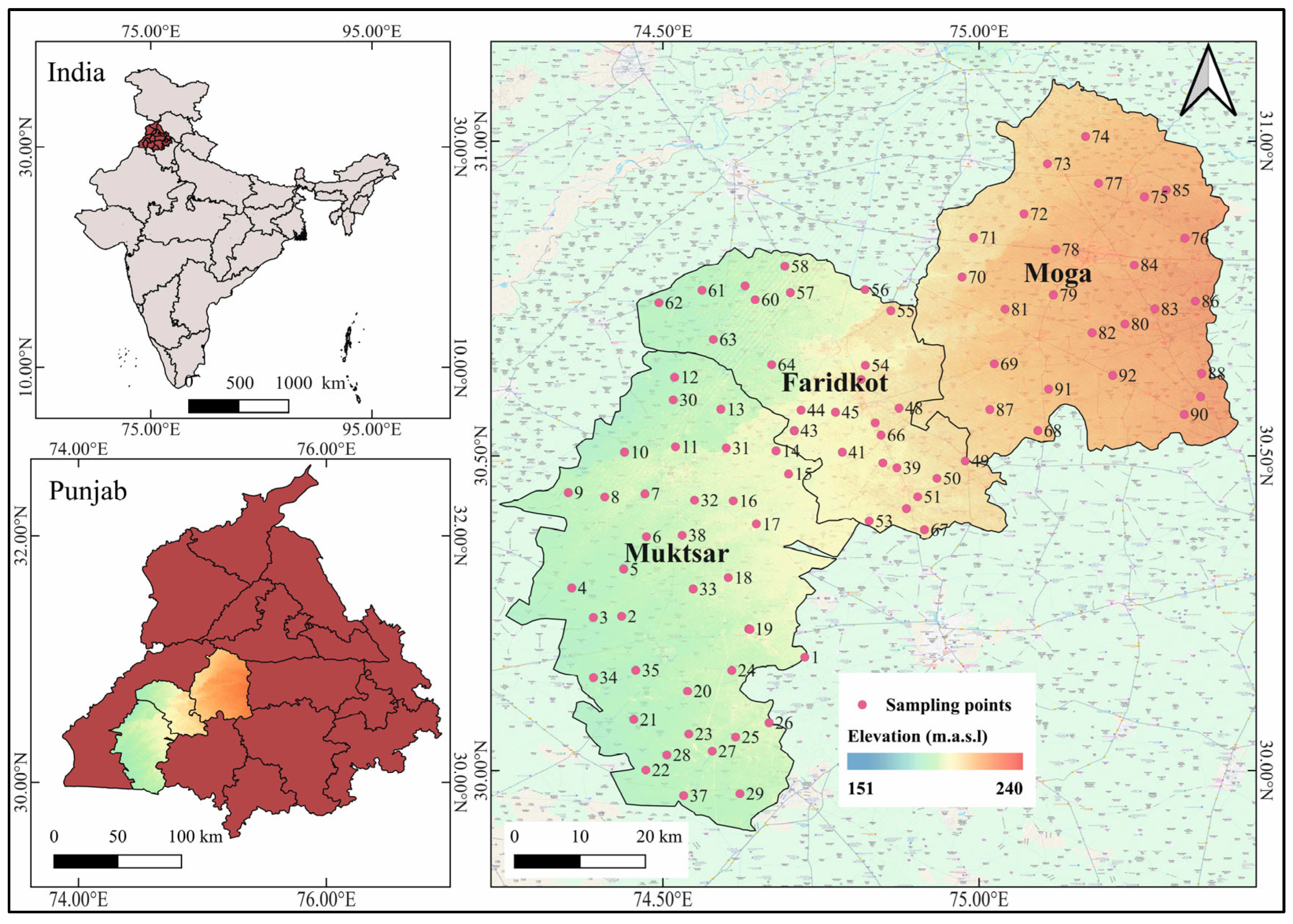
2.1. Study Area

The study area comprises three districts, viz., Faridkot, Moga, and Sri Muktsar Sahib, situated in the southwest part of Punjab, India (Figure 1). The study area is located in the western part of the Sutlej River basin and is a part of the Indo–Gangetic alluvial plain [58,59].

The elevation of the study area ranges from 151 to 240 m above mean sea level (Figure 1) [60]. The area has a hot, semiarid environment with scorching summers and chilly winters with limited precipitation. The area receives 420 mm of rainfall annually, most of which falls during the monsoon season. Moga receives the highest rainfall among these three districts [61,62,63]. The temperature varies significantly, from 1 °C in the winter to 46 °C on the hottest summer days. In terms of lithology, the region consists of Quaternary layers from the mid-Pleistocene to more recent ages [61,62,63]. These deposits are mostly composed of clay, silt, oxidized silt–clay with kankar, grey micaceous sand, and areas of loose sand that are yellowish–brown in color [61,62,63]. As the main groundwater reservoirs, the older and more recent alluvial aquifer systems are the dominating aquifer systems [61,62,63]. The soil type varies from desert and sierozem soils dominating in Moga and Muktsar, whereas Faridkot is characterized by sandy loam and alluvium [61,62,63].

In regions with little natural drainage and topographic depression, these soils are especially susceptible to salt and waterlogging because they are usually calcareous and poorly drained [61,62,63]. The groundwater of this region exhibits moderate to high levels of salt and sodicity, which poses significant hurdles to long-term irrigation use. The mineralogical composition includes feldspar, quartz, muscovite, amphibole, biotite, gypsum (anhydrite), fluorite, kaolinite, and chlorite. These minerals add to the geological diversity of the area as well as the possibility of geogenic contamination of groundwater [61,62,63].

2.2. Sampling and Analysis of Groundwater

The whole study area was divided into uniform 8 × 8 km grids, and in the period 2022–2023, 92 groundwater samples were taken 60 from shallow and from 32 deeper depths. Before sample collection, handpumps and borewells were sufficiently purged to reduce the impact of iron pipes. High-density polyethylene (HDPE) bottles that were dry and clean were used to collect the samples. Samples from each location were collected in two distinct bottles for heavy metal analysis and general water quality assessment, filled to capacity without headspace, and stored in a refrigerator at 4 °C to avoid sunlight exposure. The samples for analysis of heavy metals were filtered and acidified onsite using analytical grade 6 N HNO₃.

2.3. Physicochemical Analysis of Groundwater

The physicochemical analysis of groundwater samples was carried out using standard analytical techniques described by APHA [64]. Parameters such as pH, electrical conductivity (EC), total dissolved solids (TDS), total hardness (TH), major anions (Cl⁻, HCO₃⁻, CO₃²⁻, NO₃⁻, SO₄²⁻, F⁻), major cations (Na⁺, K⁺, Ca²⁺, and Mg²⁺), and trace elements/potentially toxic elements (PTEs) such as U, Zn, Cr, Pb, and As were analyzed for the present study [64]. The groundwater quality parameters such as pH, EC, TDS, ORP, and salinity were measured at the sampling sites using an HANNA multiparameter probe (Model HI 9829, HANNA Instruments Inc., Woonsocket, RI, USA). A flame photometer (Systronics Model 128, Systronics India Limited, Ahmedabad, India) was used to measure the levels of Na⁺ and K⁺. The EDTA titrimetric method was used to assess the levels of Ca²⁺ and Mg²⁺ in the groundwater samples [64]. The concentrations of HCO₃⁻ and CO₃²⁻ were also measured using the titrimetric method [64]. Ion chromatography (Metrohm IC Flex 930, Metrohm AG, Herisau, Switzerland) was used to analyze anions such F⁻, Cl⁻, NO₃⁻, SO₄²⁻, and PO₄³⁻. Ionic concentrations were expressed in mg/L, and the ionic balance error (IBE) was computed using the following formula to assess the analytical precision: IBE = [(ΣCations − ΣAnions)/(ΣCations + ΣAnions)] × 100.

Microwave plasma atomic emission spectroscopy (MP−AES, Agilent 4210, Agilent Technologies, Mulgrave, Victoria, Australia) was used to analyze the trace elements/PTEs which included Pb, Cr, and Zn by following the standard mode. The hydride generation method (MSIS mode) was used to analyze As in water using MP–AES. This method involved preproducing HCl and KI, then heating and diluting the mixture before forming a hydride with sodium borohydride in a sodium hydroxide matrix (Loba Chemie Pvt Ltd., Mumbai, India). The U was analyzed using an LED fluorimeter (Quantalase LF−2a, Quantalase Enterprises Pvt. Ltd., Indore, India) [65]. The 5% sodium pyrophosphate buffer (FLUREN buffer) was used to stabilize uranyl phosphate complexes, which improved the fluorescence response as well. A standard U solution (UN NO−3264, Loba Chemie, Loba Chemie Pvt Ltd., Mumbai, India) was used to calibrate the instrument, and before the analysis, a known standard was run as a sample to check the accuracy of the instrument.

2.4. Analytical Quality Assurance and Control

There were several quality control procedures used to assess the accuracy and precision of the chemical analysis. These included duplicate measurements, spiking the sample with known standard and checking the reading, and using sample blanks. The MP–AES instrument was standardized and calibrated using Multielement ICP standard solution VI (1.10580.0100, Merck, Merck KGaA, Darmstadt, Germany). The ion chromatography was calibrated and standardized using a Sigma-made multi-ion standard. The relative standard deviation (RSD) remained within 10% for all the samples. The precision of the majority of the anions was attained within ±5%.

2.5. Statistical Analysis

R software (version 4.2.3) was used to perform statistical analyses such as descriptive statistics and multivariate statistical analysis (like Spearman’s rank correlation, principal component analysis (PCA), and random forest regression (RFR)). Multivariate analyses such as Spearman’s rank correlation plot and PCA plot were used to understand the association of various groundwater quality parameters with U. The random forest model was used to predict the ranks of various groundwater quality parameters influencing the U in the groundwater.

In accordance with the methodology described by Sahoo et al. (2020) [66] and Sunkari et al. (2022) [67], the dataset was transformed using the centered log ratio (CLR) prior to PCA and random forest regression to overcome compositional data restrictions and reduce closure effects. To ensure consistency and dependability for multivariate analysis, the CLR transformation (Equation (1)) standardizes the dataset by transforming raw values into logarithmic ratios with respect to the geometric mean of the parameters:

CLR(x) = (log (x1/g(x)), log (x1/g(x))), ……………………log (xN/g(x))

(1)

Transforming correlated variables into principal components (PCs) improves PCA and helps reduce dimensionality and pattern detection. The kriging interpolation technique in QGIS (version 3.24) was used to map the regional distribution of water quality parameters, making it possible to identify hotspots and spatial trends. Moran’s I and local indicators of spatial association (LISA), together with their corresponding z-scores and p-values, were computed using GeoDa (version 1.18) software to determine the extent of spatial dependency in the groundwater U. Piper plots and Gibbs plots were prepared for hydrogeochemical characterization using Geochemist’s Workbench^® (Edition 12, Community Version) and MS Excel software (MS office Home & Student 2019).

Random Forest Regression

The RFR was employed to quantify the importance of various groundwater quality parameters in the occurrence of U in the groundwater of the study area. It is an ensemble learning technique that addresses outliers and considers interdependencies and nonlinear interactions among explanatory variables [68]. Contemporary research on forecasting groundwater pollution utilizing RF and other machine learning (ML) methodologies has highlighted the enhancement in predictive accuracy relative to traditional logistic or linear regression (LR) approaches [69,70,71,72]. Moreover, random forest models can identify significant explanatory variables and statistically elucidate their impact on pollutant occurrence in aquifers [73].

In contrast to LR, an RFR model generates many decision trees, each providing independent predictions of the model result [72]. The output of the model represents U concentrations in the groundwater, denoted as log₁₀(U). Before constructing the model, it was evaluated for correlations and dependencies among all potential parameters. Although tree-based approaches exhibit relative insensitivity to correlations among predictors, a cutoff criterion of 0.85 was employed to eliminate strongly associated predictor variables, yielding a total of 11 variables. The randomness is integrated into the model through two primary mechanisms: (1) Bootstrapped samples from the training dataset are utilized to make each tree, and the estimates of log₁₀(U) from all trees are grouped by bagging; (2) Each decision node in the tree considers a randomly chosen regressor for splitting. The quantity of trees, denoted as ntrees, and the count of regressor variables selected at each node, called as mtry. The mtry are the tuning factors that control the Overall performance of the RFR model is tuned by mtry as a tuning factor. Given that ntrees do not significantly enhance model performance beyond 100, we selected a conservative value of 500 trees for the RFR. Observations that were not randomly chosen for a decision tree are referred “out-of-bag” (OOB) samples, utilized throughout model construction to estimate error and evaluate model efficacy.

The observed log₁₀(U) to estimate the root-mean-square error (RMSE) is as follows:

$${RMSE}_{OOB}=\sqrt{{\displaystyle \frac{{\sum }_1^n{\left[y_i-{\widehat{y}}_i^{OOB}\right]}^2}{n}}}$$

(2)

“RMSE_OOB” is the RMSE of the OOB estimates, “y_i” is the observed log₁₀(U) value, “y_i^OOB” is the average projected log₁₀(U) value based on OOB samples, and “n” is ntrees. Of the total samples, 80% of them were used as tranning dataset for model calibration, while the remainder were utilized as testing datasets. The final RFR model was established using 10× cross-validation performed 5 times, with the ideal mtry value identified via a grid search method that yielded the lowest RMSE. In recurrent cross-validation, the training data are randomly divided into a 90:10% ratio, with 90% utilized for model fitting and the remaining 10% reserved for prediction by the trained model to assess the error rate. Alongside RMSE, mean absolute error (MAE), which quantifies the average deviation of predictions from actual values, and pseudo-R² values were computed during model calibration utilizing out-of-bag predictions [74]. Explanatory factors hold greater significance for log₁₀(U) when there is an increased deterioration in RMSE performance.

It was illustrated that the impacts of each regressor variable and variable sets on log₁₀(U) were plotted by plotting univariate and multivariate partial dependencies (PDs). Due to interdependencies and interactions among regressor factors, PDs may demonstrate prejudice, that can be identified by a comparison with accumulated local effect (ALE) plots, given that most variables exhibit a degree of association with others. The influence of factors (1st order) and their interactions (2nd order) on U concentrations in groundwater were assessed utilizing ALE plots [75]. The ALE plots are impartial and operate effectively even in the presence of correlated explanatory variables, in contrast to partial dependence plots [75]. The 1st order ALE plots illustrate the primary effects of a regressor in relation to the actual model prediction. The distribution of a factor is segmented into intervals according to its quantiles, and within each interval, an average discrepancy in predictions is computed [75]. The average deviations in forecasts are aggregated and centered across all intervals. The 2nd order ALE plots exclusively illustrate the supplementary impact of the association between two factors on groundwater U estimates, omitting the key effects of each factor. Consequently, if an association does not influence the concentration of U in the groundwater or if two factor do not interact, then 2nd order ALE estimates throughout the grid should approximate zero, irrespective of the presence of strong first-order effects for each variable [75]. We employed the random forest and caret packages of the R statistical programming language to perform the RFR and cross-validation [76]. Feature significance, PD, and ALE plots were produced using the iml, pdp, and ALEPlot packages, respectively [75,77]. A SMLR technique, boosted regression tree, was employed to evaluate model performance. The RFR and the boosted regression tree exhibited comparable performance, including the associations between variables and U levels in the groundwater.

2.6. Spatial Autocorrelation Using Moran’s Index

Spatial autocorrelation quantifies the extent of spatial clustering of identical attribute values, like pollutant concentrations [78]. The spatial distribution of U concentrations throughout the study area was measured using the global Moran’s I statistic, a commonly used method for measuring global spatial autocorrelation. The following formula investigates the relationship between observed values and their spatial distribution [79] (Equation (3)):

$$I={\displaystyle \frac{n}{{\sum }_{i=0}^n{\sum }_{j=1}^n{w}_{i,j}}}{\displaystyle \frac{{\sum }_{i=0}^n{\sum }_{j=1}^n{w}_{i,j\left(x_i-\overline{x}\right)\left(x_j-\overline{x}\right)}}{{\sum }_{i=0}^n{\left(x_i-\overline{x}\right)}^2}}$$

(3)

Here, “n” is the total number of observations, and “X_i” and “X_j” show the concentration of U at locations i and j, respectively. The mean of all values is $\overline{x}$. The spatial weight that indicates the relationship between locations I and J is “w_i,j”.

The Moran’s I value lies between −1 and +1. The negative number implies regional dispersion (high–low or low–high), and a positive value shows spatial clustering of selected parameters (high–high or low–low). The null hypothesis is that no spatial dependency is supported by a value close to zero, which suggests a random spatial distribution. The Moran’s Index z-score and p-value are critical parameters [80]. The z-score is calculated using the following formula (Equation (4)):

$$z-score={\displaystyle \frac{1-E\left(I\right)}{\sqrt{var\left(I\right)}}}$$

(4)

where “var (I)” is the variance and “E(I)” is the expected Moran’s I under spatial randomization. The variance and expected value are provided by Equations (5)–(8):

$$E\left(I\right)=-{(n-1)}^{-1}$$

(5)

$$var\left(I\right)={\displaystyle \frac{1}{(n-1)(n+1){\left({\sum }_{i=0}^n{\sum }_{j=1}^n{w}_{ij}\right)}^2}}\times {[n}^2{S}_1-n{S}_2+3{\left({\sum }_{i=0}^n{\sum }_{j=1}^n{w}_{ij}\right)}^2]-{\displaystyle \frac{1}{{(n-1)}^2}}$$

(6)

Here,

$$S1={\displaystyle \frac{1}{2}}{\sum }_{i=1}^n{\sum }_{j=1}^n{(w_{ij}+w_{ji})}^2$$

(7)

$$S1={\displaystyle \frac{1}{2}}{\sum }_{i=1}^n{\sum }_{j=1}^n{(w_{ij}+w_{ji})}^2$$

(8)

Here, “w_ij” corresponds to a pair of observations at positions i and j. While “w_ij ≠ 0” signifies spatial interaction between two observations, “w_ij = 0” denotes the absence of interaction between them.

The queen’s contiguity approach, which takes into account neighbors that share an edge or a vertex, was used to determine the spatial weights (w_ij), which are crucial for characterizing neighborhood interactions [80,81]. Compared to rook contiguity, which simply takes shared edges into account, this method is more inclusive [82]. Assuming intra-polygon homogeneity in U concentrations, Thiessen (Voronoi) polygons were created using GeoDa (version 1.18) for spatial configuration, assigning each observation to the closest polygon.

Following the construction of the spatial weight’s matrix according to queen’s contiguity, 999 random permutations were carried out in order to assess statistical significance [83].

2.7. Analysis of Spatial Clusters and Spatial Outliers

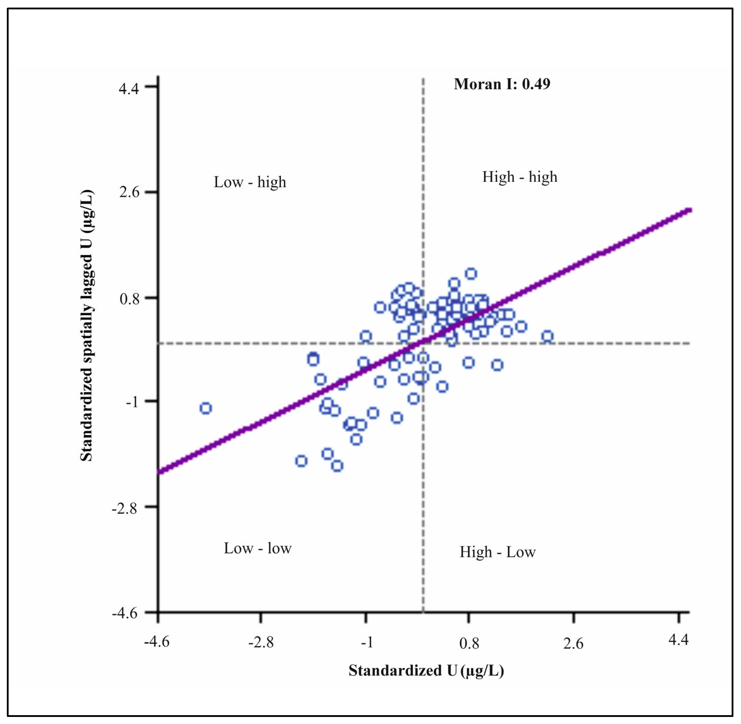
2.7.1. Moran’s Scatterplot and GIS Analysis

Geographic Information Systems (GIS) and Moran’s scatterplot were used to plot spatial patterns of U concentrations across the study area. The association in between a specific water sampling site and its surrounding sites in terms of U concentration (whether similar or divergent values are recorded in neighboring locations) is referred to as the spatial pattern in this study. Moran’s scatterplot is a statistical method for visualizing and measuring spatial autocorrelation [49].

It is predicated on bivariate linear regression, in which the measured U concentration at a specific location (x_i) is regressed on the spatially lagged variable (∑_jw_ijx_j), the weighted average U concentration of nearby locations. The global Moran’s I statistic [80], which represents the total spatial autocorrelation in the dataset, is represented by the slope of this regression line [80]. A visual comparison of the U concentration deviations and their spatial lags from the mean is made possible by the scatterplot’s zero center. Finding spatial relationships among four different quadrants is made easier by this comparison:

• High–high (HH): Areas with high U levels that are surrounded by similarly high concentrations.
• Low–low (LL): Locations with low U concentrations surrounded by similarly low values.
• High–low (HL): The U levels that are close to low levels.
• Low–high (LH): The U levels that are low and encircled by high values.

These cases, which are referred to as spatial outliers, indicate deviations from the local distribution that may be caused by distinct geological formations, patterns of land use, or sources of contamination. The CLR transformation method was used to normalize the concentration data because the validity of Moran’s I statistic rests on the assumptions of data homogeneity and normality [84,85]. This stage provides more precise interpretation of spatial patterns and confirms the robustness of statistical analysis. The analysis was performed on raw and processed data to obtain a complete picture of spatial variability.

2.7.2. Detection and GIS-Based Mapping of Key Spatial Patterns

Understanding the regional variability and possible health hazards related to U dispersion requires the identification and visualization of spatial patterns in the groundwater of the study area. Local Moran’s I statistic [86], a localized type of spatial autocorrelation that categorizes specific sampling points according to how similar or different their concentrations are to those of nearby areas, was used in this study to further enhance spatial analysis. A diagnostic technique that separates spatial clusters from spatial outliers in a dataset is called local Moran’s I. Whereas outliers indicate areas where the observed concentration differs noticeably from that of its neighbors, clusters show areas, where groundwater quality displays homogenous characteristics, such as consistently high or low U levels. The following formula is used mathematically to determine the local Moran’s I [87] (Equation (9)):

$$I_i={\displaystyle \frac{x_i-\overline{x}}{{\sigma }^2}}{\sum }_{j=1,j\ne i}^n\left[w_{ij}\left(x_j-\overline{x}\right)\right]$$

(9)

Here, “X_i” and “X_j” are the U concentration at locations i and j, respectively. The $“\overline{x}”$ is the mean concentration, and $“{\sigma }^2”$ represents variance.

To test the hypothesis and evaluate the null hypothesis, the p-value is computed [79]. It shows the likelihood that the dataset is statistically significant as compared to random chance of occurrence and calculated, as follows (Equation (10)):

$$p=P(Z\ge \left|Z_{observed}\right|)$$

(10)

where the probability of the observed z-score will be equal to or greater than the observed one. Because it demonstrates the existence of spatial autocorrelation in the dataset, a p < 0.05 means that the value of Moran’s I deviates from what would be predicted under the null hypothesis, and vice versa.

2.8. Health Risk Assessment

Assessing human health risks involves identifying the types and probabilities of adverse health effects in individuals exposed to contaminants. The primary routes through which people are exposed to groundwater contaminants include oral ingestion and dermal adsorption. Oral consumption is recognized as the main pathway for exposure to groundwater contaminants. The average daily intake (ADI) of elements in water from ingestion and dermal adsorption was calculated using Equations (11)–(14) [88].

$${ADI}_{oral}={\displaystyle \frac{C\times {IR}_{ing}\times EF\times ED}{BW\times AT}}\times {10}^{-6}$$

(11)

$${ADI}_{dermal}={\displaystyle \frac{C\times SA\times SAF\times ABS\times EF\times ED}{BW\times AT}}\times {10}^{-6}$$

(12)

In this context, “C” denotes the concentration of contaminants present in the groundwater (mg kg⁻¹); “ADI_oral” and “ADI_dermal” refer to the average daily intake values derived from groundwater ingestion and dermal adsorption (mg kg⁻¹ day⁻¹); “EF” indicates the exposure frequency, quantified as 350 days per year⁻¹; “ED” represents the exposure duration (67 years for adult male and female, and 12 years for children) [89,90]; and “IR_ing” signifies the ingestion rate (mg day⁻¹). “SA” represents the exposed skin area (5700 cm² for adults and 2800 cm² for children) [90]. “BW” refers to body weight (65 kg for adult, and 15 kg for children). Ultimately, “AT” represents the averaging time, calculated as lifetime × 365 days for carcinogens (As, Cr, and Pb), and “ED” × 365 days for noncarcinogens [90].

Noncarcinogenic Health Risk

The hazard quotient (HQ), estimated as the ratio of ADI to the reference dose (RfD), is articulated in Equation (13) [88]. It is frequently used to assess the noncarcinogenic risks.

$$HQ={\displaystyle \frac{ADI}{RfD}}$$

(13)

where “RfD” denotes the reference dosage (mg kg⁻¹ day⁻¹) of groundwater contaminants presented in Supplementary Table S1. This denotes the highest concentration of a contaminant that is considered safe for human health.

The USEPA (2002) [89] provides a method for assessing skin absorption exposure to contaminants without reference dosages. This method entails multiplying the groundwater oral reference dosage by a gastrointestinal absorption coefficient to ascertain dermal risk [90].

To assess the cumulative noncarcinogenic impacts of various groundwater contaminants, the hazard index (HI) is determined by summing the hazard quotient (HQ) values of each PTE. The formula for HI is represented as Equation (14) [90].

$$HI=\sum {HQ}_i=\sum {\displaystyle \frac{{ADI}_i}{{RfD}_i}}$$

(14)

Here, “HQ_i” signifies the Hazard Quotient for the i^th element, “ADI_i” indicates average daily intake, and “RfD_i” specifies the reference dose for the corresponding element. If the HI < 1, it is improbable that the exposed individual will have adverse health effects. Conversely, if the HI value exceeds 1, there is a potential for a noncarcinogenic health effect, with the likelihood increasing alongside the HI value [89].

3. Results and Discussion

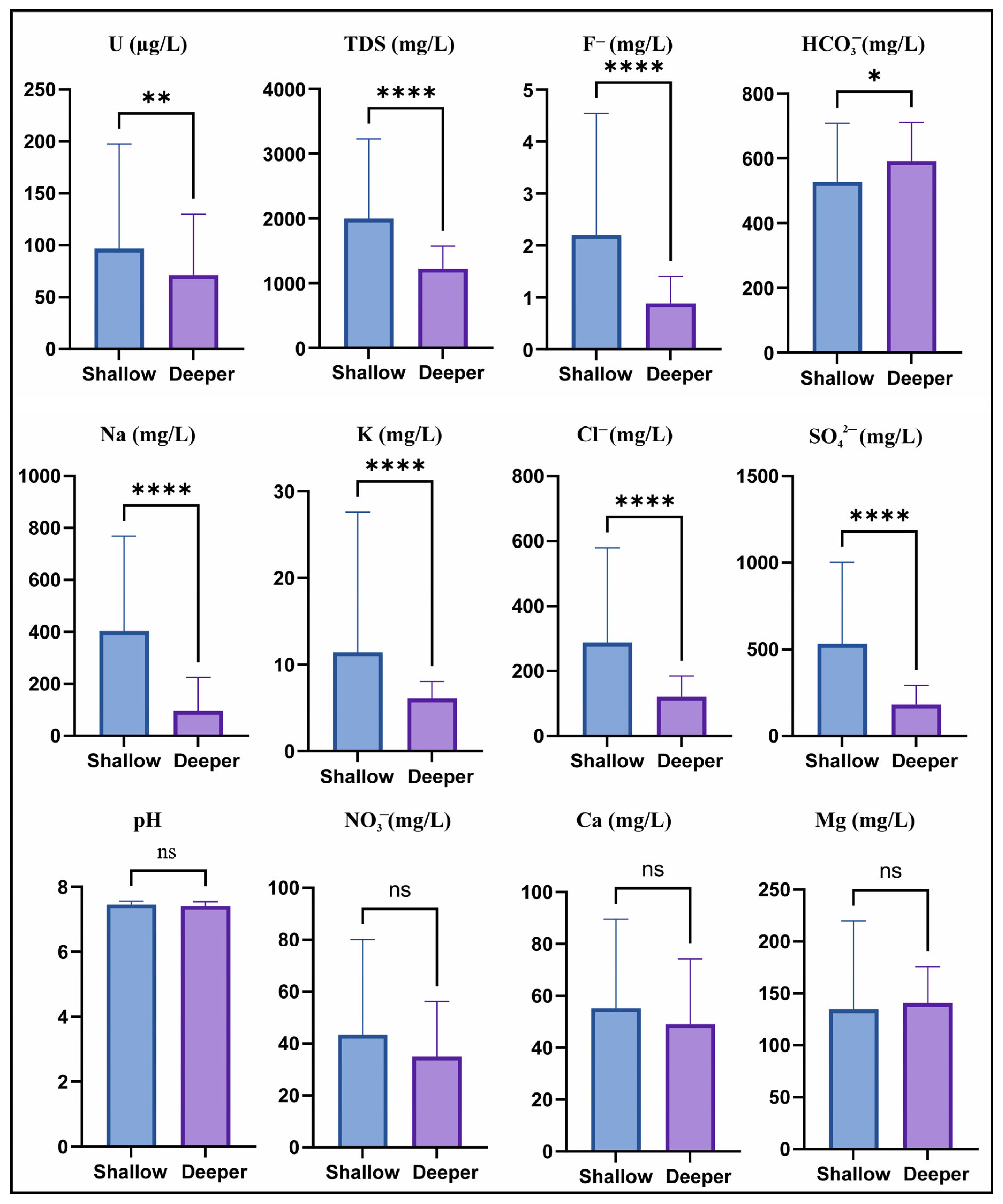
3.1. Distribution of Groundwater Quality Parameters in Shallow and Deeper Groundwater

The descriptive statistics of the physicochemical properties in the groundwater of both shallow and deeper depths are given in

Table 1. Descriptive statistics of groundwater physicochemical properties in shallow and deeper groundwater. This Table shows that the descriptive statistics of groundwater quality parameters with % samples exceeding the WHO limit in shallow and deeper depth.

Parameters	Units	Min	Max	Med	Avg	SD	Min	Max	Med	Avg	SD	Permissible Limit [92]	% Samples > Permissible Limit
			Shallow (<180 ft)					Deeper (>180 ft)					Shallow	Deeper
pH		6.7	8.2	7.4	7.4	0.33	6.9	8.3	7.4	7.4	0.35	6.5–8.5	0	0
EC	μS/cm	312	9147	2967	3371	1889	275	4236	1250	1632	988.6		−	−
TDS	mg/L	208	6397	2016	2339	1324.8	184.2	2843	837.5	1094.5	663.8	500	97	81
ORP	mV	12.8	215	151	118.3	72.5	23.7	218	151	124.3	70.5		−	−
Salinity	mg/L	30.7	2780	635	730.1	683.2	117	1230	530	572	241.4		−	−
HCO3−	mg/L	100	1200	500	491	166.7	200	1000	500	507.6	154.6	200	91	93
F−	mg/L	0.3	14.4	1.7	2.2	2.3	0.3	1.98	0.8	0.9297	0.41	1.5	54	15
Cl−	mg/L	10.37	1507.81	180.48	276.93	292.3	12	240	31	59.54	65.9	250	35	0
NO3−	mg/L	1.143	166.86	28.61	38.94	31.7	4.34	35	18	18.22	8.4	50	25	0
SO42−	mg/L	16.54	1936.14	404	525.64	466.7	31	529	164	179.8	114.8	200	74	36
Na	mg/L	6.98	1540.14	320.7	409.83	363.2	2.9	440.9	25.2	99.03	131.7	200	66	18
K	mg/L	2.04	105.66	8.02	12.45		2.56	11.5	6	6.181	1.9		−	−
Ca	mg/L	6.4	600	65.6	109.4	118	0	405	135	135.5	92.8	75	45	72
Mg	mg/L	20.32	1255.5	228	316.3	277.9	279	961	558	551.4	160.4	30	91	100
Zn	μg/L	BDL	50.1	13.9	17.4	17.6	BDl	31.8	5.1	7.8	9.4	5000	0	0
Pb	μg/L	BDL	7	0	0.9	2.3	BDL	7	0	0.9	2.3	10	0	0
As	μg/L	BDL	6.9	0	3.4	2.7	BDL	8.2	0	3.1	4.1	10	0	0
U	μg/L	0.6	456.65	62.87	95.81	98.02	8.14	349	60.9	75.5	65.7	30	76	84

Notes: Min: minimum; Max: maximum; Avg: average; SD: standard deviation; EC: electrical conductivity; TDS: total dissolved solids; ORP: oxidation reduction potential.

. Results indicate a significant difference between average and median values for various groundwater quality parameters, which exhibited greater standard deviation (SD). Generally, the standard deviation for various parameters in shallow groundwater was higher than that groundwater quality parameters in deeper groundwater. The pH varied from 6.7 to 8.3, with a median pH of 7.4 for both shallow and deeper groundwater (Table 1), and all the sample pH was within the permissible limit (WHO: 6.5 to 8.5). This indicates the slightly alkaline nature of the groundwater in the study area. This is due to the prevalence of carbonate minerals in the sediments of the study area. The slightly alkaline nature of groundwater in several regions of Punjab, India, has also been reported by other researchers [18,56,57]. Shallow groundwater exhibited higher salinity (median: 635 mg/L) compared to deeper groundwater (median: 530 mg/L). Similarly, elevated TDS was observed in shallow water (208–6397 mg/L; 97% > WHO drinking water permissible limit) in contrast to deeper water (184.2 to 2843 mg/L; 81% > WHO drinking water permissible limit) (Table 1). It can be attributed to increased weathering and salt dissolution, alongside anthropogenic contributions, facilitated by the rapid recharge of water through shallow aquifers. According to the groundwater classification of Freeze and Cherry [91], both shallow and deep groundwater are predominantly categorized as brackish (1000 < TDS < 10,000 mg/L). The TDS and salinity were higher in the groundwater samples from shallow depths than from deeper depths, as reported by many studies in the context of Punjab, India [56,57]. The ORP ranged from 12.8 to 215 mV (median 151 mV) in shallow groundwater and from 23.7 mV to 218 mV (median 151 mV) in deeper groundwater (Table 1), signifying the prevalence of oxic conditions; nevertheless, very few (<10% of samples) exhibited sub-oxic and more reducing conditions at deeper depths.

The shallow groundwater was primarily dominated by cations such as Na, Mg, and Ca, and anions such as SO₄²⁻, Cl⁻, HCO₃⁻, and NO₃⁻, whereas the deeper groundwater was predominantly dominated with cations such as Mg, Na, and Ca, along with anions HCO₃⁻, SO₄²⁻, Cl⁻, and NO₃⁻. The average concentrations of Na, K, Ca, Mg, HCO₃⁻, SO₄²⁻, Cl⁻, and NO₃⁻ in groundwater from shallow depths were 409.83 mg/L, 12.45 mg/L, 109.4 mg/L, 316.3 mg/L, 491 mg/L, 525.64 mg/L, 276.93 mg/L, and 38.94 mg/L, respectively. The average concentrations of these ions in groundwater from deeper depths were 99.03 mg/L, 6.18 mg/L, 135.5 mg/L, 551.4 mg/L, 507.6 mg/L, 179.8 mg/L, 59.54 mg/L, and 18.22 mg/L, respectively (Table 1). The groundwater quality parameters such as Na, Ca, Mg, HCO₃⁻, SO₄²⁻, Cl⁻, and NO₃⁻ exceeded the WHO drinking permissible limit in 66%, 45%, 91%, 91%, 74%, 35%, and 25% of samples from shallow depth, respectively, whereas the Na, Ca, Mg, HCO₃⁻, SO₄²⁻, and NO₃⁻ concentrations exceeded the permissible limit in 18%, 72%, 100%, 93%, 36%, and 36% of samples, respectively, from deeper depths (Table 1). Some previous studies also reported higher concentrations of major cations and anions in the groundwater of the Malwa region of Punjab [18,56]. The concentrations of U (range: 0.6 to 456.5 μg/L) and F⁻ (range: 0.3 to 14.4) were more elevated in shallow groundwater than in deeper groundwater (Table 1). Uranium exceeded the drinking water permissible limit in 76% and 84% of groundwater samples from shallow and deeper depths, respectively. The concentration of F⁻ exceeded the drinking water permissible limit in 54% and 15% of groundwater samples from shallow and deeper depths, respectively (Table 1). Other trace elements/heavy metals such as Zn, Pb, and As were within the permissible limits in all the samples from both shallow and deeper groundwater (Table 1). It is significant to observe that major ions concentrations were more elevated in the groundwater samples from shallow depths than from the deeper depths (Table 1). Based on the Wilcoxon signed rank test, the p-values for U, TDS, F⁻, HCO₃⁻, Na, K, Cl⁻, and SO₄²⁻ concentrations were 0.0071, <0.0001, <0.0001, 0.0105, <0.0001, <0.0001, <0.0001, and <0.0001; these are significantly less than p = 0.05, which indicates that there is a significant difference between shallow and deeper groundwater for U, TDS, F⁻, HCO₃⁻, Na, K, Cl⁻, and SO₄²⁻ concentrations in the study area (Figure 2). Meanwhile, the p-values of pH, NO₃⁻, Ca, and Mg concentrations were 0.4069, 0.4471, 0.8203, and 0.8696; these are significantly greater than p = 0.05, which indicates that there is no significant difference between shallow and deeper groundwater for pH, NO₃⁻, Ca, and Mg concentrations in the study area (Figure 2).

3.2. Hydrogeochemistry of Groundwater of the Study Area

Piper trilinear plots and Gibbs plots were prepared to understand the origins of major ions and the dominant hydrogeochemical processes governing groundwater chemistry in the study area, as presented in the Figure S1a,b [93,94]. Figure S1a illustrates that around 75% of the samples of the groundwater from deeper depth were categorized as Mg−HCO₃⁻ type, and the remaining 25% of the samples were classified as alkali and alkaline earth types. The prevalence of Mg−HCO₃⁻ species associated with lower salinity in the groundwater at deeper depth indicates that rock weathering is the major governing factor controlling groundwater chemistry (Figure S1b). In shallow groundwater with elevated salinity, the predominant Mg−HCO₃⁻ species decreases when mixed facies, including Na−HCO₃⁻, Na−Cl⁻, and Mg−Cl⁻ types, increase; a comparable finding was reported by Chandrasekar et al. (2021) [93]. This may be due to increased interaction between surface and groundwater, heightened agrochemical contributions from surface waters, and the influence of evaporation. The mixing process may result in the desorption and/or dissolution of additional secondary minerals, including salts, in the shallow aquifers [57]. Figure S1b illustrates that elevated TDS in shallow depth results from the predominance of evaporite weathering, while elevated TDS in deeper groundwater is attributed to the dominance of rock–water interactions.

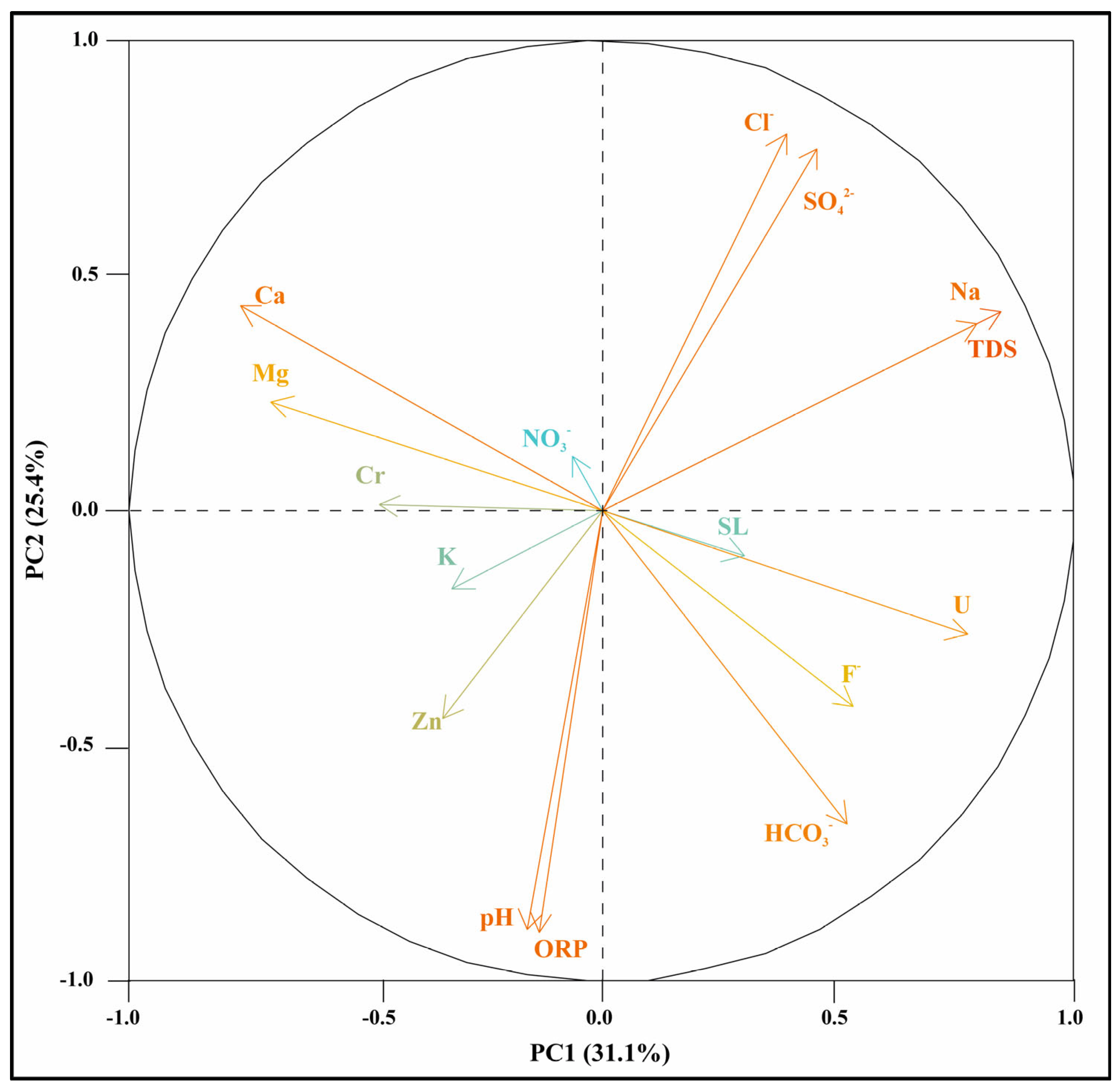
3.3. Multivariate Statistical Analysis

To understand the role of various groundwater quality parameters in the occurrence and mobilization of U in the groundwater from shallow and deeper depth, Spearman’s rank correlation and PCA plots were prepared. Spearman’s rank correlation plots often quantify the degree of association between selected parameters (Figures S2 and S3). Correlation strengths were categorized as follows: very weak (ρ = 0 to ±0.1), weak (ρ = ±0.1 to ±0.39), moderate (ρ = ±0.4 to ±0.69), and strong (ρ = ±0.7 to ±0.9). Uranium exhibited a moderate positive correlation with TDS (ρ = 0.68), SL (ρ = 0.67), HCO₃⁻ (ρ = 0.53), F⁻ (ρ = 0.49), SO₄²⁻ (ρ = 0.46), and Na (ρ = 0.47) in shallow groundwater (Figure S2), while it showed a moderate positive correlation with F⁻ (ρ = 0.54), TDS (ρ = 0.47), SL (ρ = 0.48), and HCO₃⁻ (ρ = 0.55), and a weak positive correlation with NO₃⁻ (ρ = 0.36), Na (ρ = 0.25), and Cl⁻ (ρ = 0.21) in deeper groundwater (Figure S3). Fluoride was moderately positively associated with TDS (ρ = 0.54), Cl⁻ (ρ = 0.45), SO₄²⁻ (ρ = 0.5), and Na (ρ = 0.53) in shallow groundwater (Figure S2), but in deeper groundwater, it showed a moderate positive correlation with TDS (ρ = 0.61), SL (ρ = 0.57), Cl⁻ (ρ = 0.44), Na (ρ = 0.45), and K (ρ = 0.43) (Figure S3). Shallow groundwater TDS exhibited a significant positive correlation with Cl⁻ (ρ = 0.87), SO₄²⁻ (ρ = 0.82), and Na (ρ = 0.84), while demonstrating a moderate positive correlation with HCO₃⁻ (ρ = 0.4), K (ρ = 0.53), and Ca (ρ = 0.42) (Figure S2). The TDS in deeper groundwater exhibited a significant positive correlation with SL (ρ = 0.99), Cl⁻ (ρ = 0.89), and Na (ρ = 0.55), and a moderate positive correlation with HCO₃⁻ (ρ = 0.61), SO₄²⁻ (ρ = 0.35), and K (ρ = 0.5) (Figure S3). Uranium and F⁻ negatively correlated with Ca in shallow and deeper groundwater (Figures S2 and S3). Uranium had a weak positive correlation with pH in both shallow and deeper groundwater, while F⁻ showed a weak positive correlation with pH (ρ = 0.12) in shallow groundwater and a moderate positive correlation with pH (ρ = 0.37) in deep groundwater (Figures S2 and S3). Similarly, numerous investigations in nearby districts to the study area have previously reported the positive association of U with TDS, SL, HCO₃⁻, F⁻, SO₄²⁻, and Na in the groundwater [18,57,95].

Consequently, the PCA plots also ascertained the characteristics and origins of contaminants in groundwater. In clr-transformed PCA, five principal components (PCs) with eigenvalues > 1 were identified, accounting for 80.1% of the total variance, as presented in Figure S4. The initial two PCA axes collectively represented 56.5% of the total variance, with PC1 contributing 31.1% and PC2 contributing 25.4% (Figure 3). The PCA biplot demonstrated that PC1 accounted for 31.1% of the total variance and was positively loaded with TDS, SL, F⁻, Cl⁻, SO₄²⁻, U, HCO₃⁻, and Na (Figure 3). This is due to dissolution of minerals into the groundwater in the study area (Figure 3) [96]. Sharma et al. (2017) [97] reported that geogenic processes, such as gypsum dissolution and the weathering of silicate-rich rocks, can release SO₄²⁻ into groundwater, contributing to its weak to strong positive correlation with TDS, SL, Na, and Cl⁻ (ρ = 0.3 to 0.88) (Figures S2 and S3) [97]. Singh et al. (2011) [98] and Rasool et al. (2018) [99] reported that the presence of F⁻ in groundwater results from the dissolution of F⁻−bearing minerals such as fluorite, mica, and topaz in an alkaline condition. In alkaline environment interaction schists, quartzites, and granites with water results in the Na enrichment in the groundwater of this region [40]. Weathering of rocks containing the calcite, dolomitic limestone, silicate, calcareous slates can be regarded as potent sources of SO₄²⁻, HCO₃⁻, and Mg in the groundwater of this region [40,100]. The PC2 accounted for 25.4% and had significant positive loadings with Cl⁻, SO₄²⁻, Ca, Mg, and Na, alongside a negative loading of pH (Figure 3).

The presence of these groundwater quality parameters in the same group indicates a shared origin (Figure 3). Most of the PC2 components exhibited moderate association with one another, supported by Spearman’s rank correlation analysis. Hundal et al. (2012) [101] have also reported the leaching of SO₄²⁻ from fertilizers and other anthropogenic activities [101]. The sandy loam soil in this location significantly contributes to the increased SO₄²⁻ load from surface precipitation via irrigation and rainfall [102]. The primary sources of U in the study area are most probably geogenic, especially weathering of granitic rocks, with a subordinate influence from anthropogenic factors such as groundwater table decline and fertilizer application [54,57,103,104,105,106]. The Bhabha Atomic Research Centre (BARC) report asserts the presence of U in phosphate fertilizers (70 to 100 mg/kg) utilized in the Punjab, India [104]. Uranium present in fertilizers can introduce U into groundwater through percolation with irrigation water [105]. Therefore, the potential for U leaching from fertilizers to contaminate groundwater in the shallow aquifer in study area cannot be dismissed.

The notable correlation of U with HCO₃⁻ in Spearman’s rank correlation analysis (ρ = 0.53) for shallow groundwater and (ρ = 0.55) for deeper groundwater, coupled with alkaline pH, elevated HCO₃⁻ levels, and high TDS in the study area, substantiates the mechanism of U leaching and mobilization from soils and sediments into groundwater [53,105,106,107,108,109]. High TDS resulting from high salt concentrations leads to the formation of soluble U complexes due to excessive ion exchange reactions, which are key drivers of U solubility in aquifers [53,108,109]. In the oxic and alkaline environment U tends to form uranyl-carbonate complexes and mobilize into the groundwater [109]. Because these anions do not readily adsorb to mineral surfaces at basic pH, these carbonate species may facilitate the desorption of U from mineral surfaces. Also, competition of HCO₃ ⁻ with U oxyanions for sorption sites of Fe-oxides/ oxyhydroxides results in U mobility [53,109].

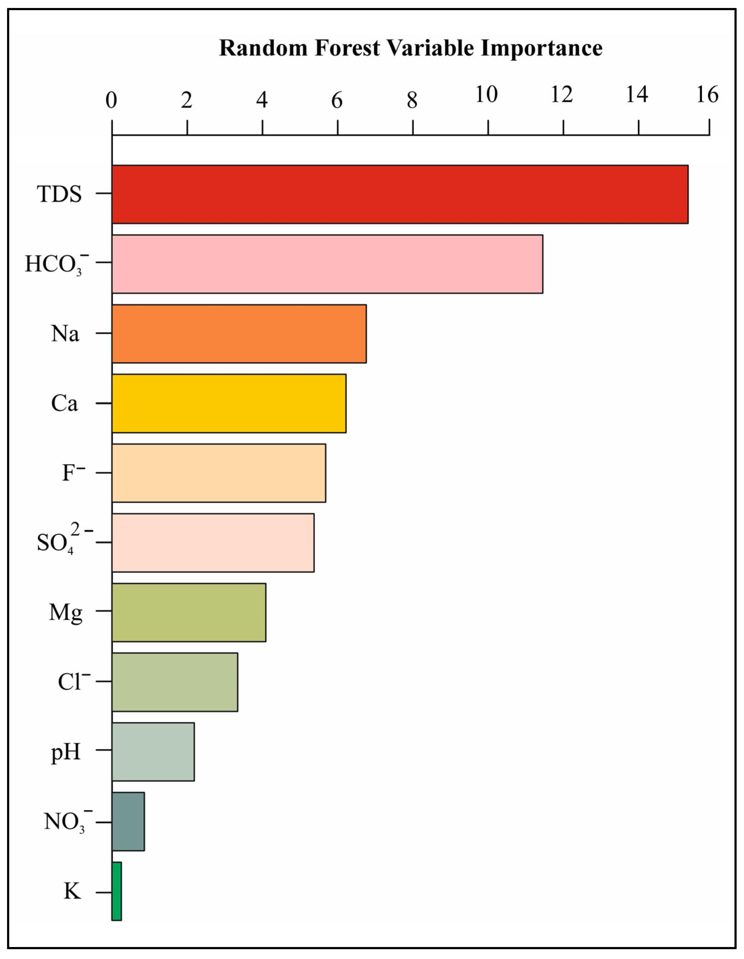
Prediction of Important Groundwater Quality Parameters Controlling Occurrence of U in the Groundwater Using Random Forest Model

Groundwater quality parameters were ranked in order of significance based on their effects on RMSE performance in the random forest model (RF) (Figure 4). Groundwater TDS was the most prominent factor in the RF model, followed by HCO₃⁻, Na, and F⁻, SO₄²⁻, Mg, Cl⁻, pH, NO₃⁻, and K concentrations (Figure 4). A positive association of U with TDS, HCO₃⁻, Na, F⁻, SO₄²⁻, Mg, Cl⁻, pH, NO₃⁻, and K can be also seen in Spearman’s correlation plots and PCA plots (Figures S2 and S3). The results are consistent with previous observations which reported that HCO₃⁻ alkalinity and TDS are prominent parameters controlling the groundwater U concentrations [57,106,110,111,112]. The geogenic contamination of U in the groundwater has been suggested to be associated with HCO₃⁻-rich water [112]. Remarkably, in RF model, HCO₃⁻ in the groundwater has been estimated as the 2nd most important factor influencing U concentration in the groundwater [106,111,112]. In present study, dissolved Ca may have a strong impact on groundwater U predictions, which suggests that the uranyl–Ca–carbonate complexes, rather than only carbonate complexes, are likely the major influences on groundwater U [106,111,113]. In addition to dissolved Ca and HCO₃⁻, groundwater pH and dissolved Na contents vastly contributed to prediction of U in the groundwater (Figure 4) [113]. In agriculturally influenced aquifers of the study area, a moderate positive correlation of U with SO₄²⁻ (sulphate from solution (which occurs via dissimilatory sulphate reduction)) indicates reducing conditions where U(IV) is stable, limiting its solubility [56,57,95,114]. The SO₄² present in the groundwater serves as the most significant redox indicator in this model [114].

Riedel and Kubeck (2018) [115] also noted that SO₄²⁻-reducing conditions resulted in near-zero probabilities of U contamination in groundwater, and higher redox potentials associated with NO₃⁻ presented the greatest probability of elevated U. Nitrate is a direct U(IV) oxidant and is presumed to partly control U presence in groundwater [116].

Nitrate is produced mainly through the nitrification of ammonium-based and organic fertilizers, as well as from animal waste. It is highly leachable, which has important implications for environmental management [106,111,117]. Consequently, whereas NO₃⁻ acts as an oxidant for U(IV), the simultaneous presence of U and NO₃⁻ in groundwater may results from their analogous mobilities and movement alongside (irrigation) recharge water [117]. Fluoride, SO₄²⁻, and Mg moderately controlled the U enrichment in the groundwater of the study area, presented in Figure 4. The concentrations of Cl⁻, pH, NO₃⁻, and K weakly control the U enrichment in the groundwater (Figure 4). Weak positive associations of U with pH, NO₃⁻, and Cl⁻ are also reported in various studies nearby the study area [18,56].

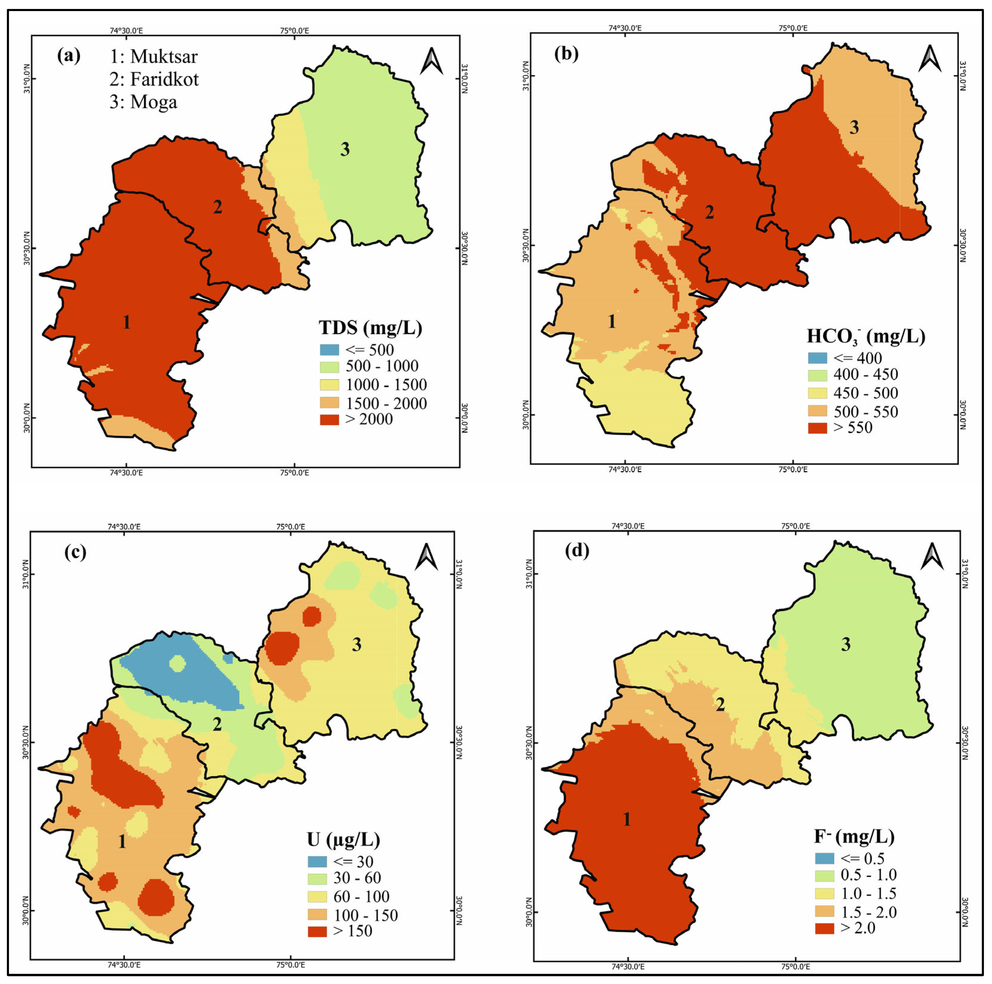
3.4. Geospatial Distribution of TDS, HCO₃⁻, U, and F⁻ in the Groundwater

The geospatial distribution of TDS, HCO₃⁻, U, and F⁻ is illustrated due to the substantial positive correlation of U with TDS, HCO₃⁻, and F⁻, as presented in Figure 5. The TDS concentration is decreasing from the southwest to the northeast region of the study area (Figure 5a). A transition zone has been observed in the Faridkot district. Similarly, the HCO₃⁻ concentration is higher than the permissible limit in the whole area but higher in the middle part than in the northeast and southwestern parts (Figure 5b). Figure 5 clearly shows that the concentration of U is increasing from the northeast part of the study area to the southwest region. The concentration of U was found to be <30 µg/L in the northern part of Faridkot due to the mixing of surface water into the groundwater from a dense canal network. The concentration of F⁻ also follows the same pattern as TDS. It can be seen that areas with higher concentrations of U are also dominated by TDS, HCO₃⁻, and F⁻ in the groundwater (Figure 5).

3.5. Moran’s I and Spatial Autocorrelation

Moran’s I is a significant spatial statistical measure utilized to determine the existence or nonexistence of spatial autocorrelation, consequently influencing the selection of spatial statistical methodologies [118]. Nonetheless, Moran’s I is primarily a statistical measure rather than a mathematical construct. The value of Moran’s I ranges from −1 to +1 [119]. A negative number indicates geographical dispersion (high–low or low–high), while a strongly positive value denotes spatial clustering of similar values (high–high or low–low). The null hypothesis positing the absence of geographical dependency is corroborated by a value near zero, indicating a random spatial distribution [80]. Figure 6 shows a significant positive value of Moran’s I for U in the groundwater of the study area, which represents the clustering of U in the groundwater. For U, most samples fall in the categories of high–high and low–low (Figure 6).

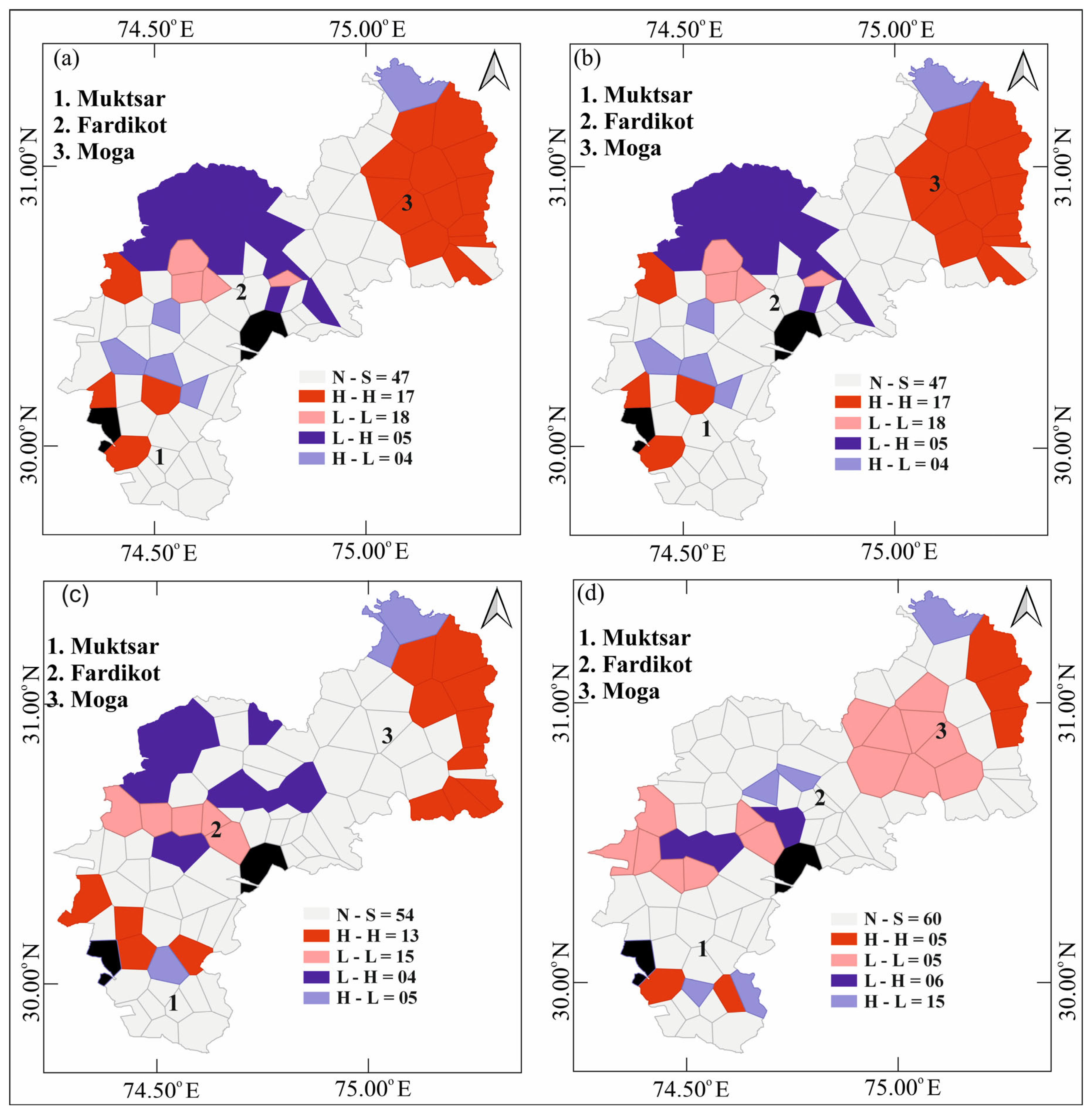
Spatial Clusters and Spatial Outliers’ Identification and Mapping

Before identifying notable regional U hotspots and cool spots, Moran’s I scatterplots and GIS analysis were employed to examine prospective spatial clusters (low–low and high–high) and spatial outliers (high–low and low–high). The outcomes of spatial autocorrelation are influenced by the spatial weight function, the existence of extreme values, and the nonnormality of the data [120]; thus, this study utilized the transformed dataset (n = 91). Potential patterns were analyzed using the q1, q2, q3, and q4 queen’s spatial weight matrix.

Table 2. Number of potential patters in U distribution in groundwater of the study area.

Data Treatment	High–High	High–Low	Low–High	Low–Low	Not Significant
		U
CLR transformed, q1	17	18	4	5	47
CLR transformed, q2	17	18	4	5	47
CLR transformed, q3	13	15	5	4	54
CLR transformed, q4	5	5	15	6	60

illustrates the number of substantial spatial patterns (high–high and low–low) were identified. Figure 7 illustrates that the high–high potential spatial patterns for U were situated in the northeastern region of the present study. It was also expected that substantial spatial patterns were influenced by the configuration of the spatial weight matrix. As the order of queen’s contiguity increased, the low–high spatial patterns transitioned from the Faridkot district to the Muktsar district for U. The univariate local indicator of spatial autocorrelation (LISA) was employed to detect and delineate significant geographical clusters and spatial outliers. The computation relied on Equation (7), and, due to the incorporation of mean and variance, the transformed dataset was utilized to mitigate issues related to skewed data in spatial cluster and spatial outlier analysis [80]. The global Moran’s I index of U in the groundwater was calculated using q1 queen’s contiguity (Figure 6). A substantial positive Moran’s I value of 0.49 was obtained for U (Figure 6). The outcomes of spatial analysis were influenced by the number of neighbors; hence, the computation of the LISA was conducted at elevated orders for all site.

Table 3. Statistical significance test of spatial clusters and spatial outliers. Positive Moran’s I and z-score values represent significant spatial patterns.

Data Treatment	Moran’s I	SD	E	z-Score	p-Value
		U
CLR transformed, q1	0.49	0.06	−0.01	7.8	0.001
CLR transformed, q2	0.35	0.04	−0.01	7.4	0.001
CLR transformed, q3	0.18	0.04	−0.01	4.6	0.001
CLR transformed, q4	−0.12	0.03	−0.01	−2.3	0.009

presents the overall findings of statistical significance tests conducted to estimate spatial patterns via 999 permutations. Compared to the results obtained from assessing prospective spatial patterns using Moran’s I scatterplot and GIS in Figure 6, the number of substantial spatial clusters decreased as the order of the queen’s contiguity increased. Using queen’s contiguities’ (q1, q2, q3, and q4) spatial weight matrices, 18.68% (n = 17), 18.68% (n = 17), 14.28% (n = 13), and 5.49% (n = 5) of water samples were respectively identified as significant high–high spatial clusters for U. The number of water samples classified as substantial spatial outliers (low–high and high–low) remained unaffected by the increasing order of the queen’s contiguity, with the exception of q4. The magnitude of the relevance of low–high spatial outliers was increased with increasing order of the spatial weight matrix. A notable high–low spatial outlier was present near the major low–low spatial cluster (Figure 7b,c). Most of the notable high–high spatial clusters for U were found in the northeastern region of the study (Figure 7).

3.6. Human Health Risk

The hazard quotient (HQ) of an element is utilized to assess the noncarcinogenic health risk to humans. According to the USEPA, an HQ > 1 indicates a potential risk, while an HQ < 1 signifies no risk [121]. The HQ of all elements was <1 for children and adults, except F⁻, NO₃⁻, and U. The average HQ value of F⁻ is 1.51 for children and 1.12 for adults, respectively (Table S2). The average HQ values for U are 7.55 and 5.59, while for NO₃⁻ they are 1.33 and 9.99 for children and adults, respectively (Table S2). Approximately 47.86% and 41.3% of samples pose risks to children and adults, respectively, due to F⁻ contamination. About 93.49% and 89.14% of samples pose a risk to children and adults, respectively, due to U contamination, whereas 51.08% and 39.13% of samples pose a risk to children and adults, respectively, from NO₃⁻ contamination. U poses a higher risk in the study area than F⁻ and NO₃⁻.

The total noncarcinogenic risk was determined by summing the HQ of all elements in the specific sample. An HI > 1 indicates a potential risk to the population, but an HI < 1 signifies no risk to the people. The majority of the samples exhibit HI > 1, indicating a substantial noncarcinogenic risk to the population residing in the study area. Additionally, the value of HI is categorized into four classes. Risk categories include no risk, low risk, medium risk, and high risk, corresponding to HI values of HI < 1, 1 < HI <5, 5 < HI < 10, and HI > 10, respectively. In the study area, 21.74% of samples present a low risk to children and 42.39% to adults. Approximately 43.48% and 33.70% of samples present a medium risk to children and adults, respectively, whereas 34.78% and 22.83% of samples present a high risk to children and adults, respectively, in the study area. Results indicate that children are at higher risk compared to adults [114,122,123]. The comparatively low body weight of children, in contrast to adults, may contribute to heightened health risks. Early exposure to fluoride might adversely affect dental and skeletal development [122].

Groundwater has been categorized into two types according to F⁻ content and associated health risks: Class 1: F⁻ concentrations of 1.5–4 mg/L in drinking water result in dental fluorosis; Class 2: F⁻ concentrations over 4 mg/L led to dental, skeletal, and debilitating fluorosis [124]. This study indicates that 36% of groundwater samples are associated with a risk of dental fluorosis for consumers. Additionally, 14% of class 2 groundwater samples present risks of dental, skeletal, and debilitating fluorosis. These findings underscore the importance of monitoring groundwater quality to safeguard public health.

4. Conclusions

The present study revealed that the concentrations of U along with other major cations and anions were exceeded the drinking water permissible limit recommended by the WHO in most of the groundwater samples, with higher levels in the shallow depths. The major ion chemistry of groundwater in the region is predominantly influenced by carbonate weathering. PCA analysis revealed that U is positively loaded with TDS, SL, F⁻, Cl⁻, SO₄²⁻, U, HCO₃⁻, and Na on PC1. This may suggest that these are the influencing the occurrence of U in the groundwater. A significant positive association between U and TDS and HCO₃⁻ suggests that the weathering of carbonates promotes the leaching of U from aquifer materials into groundwater. Furthermore, random forest model results revealed that TDS and HCO₃⁻ are the most influential factors for U occurrence in the groundwater. To find the hotspots and cool spots of U in the study area, spatial autocorrelation plots were prepared. Spatial autocorrelation plots demonstrated that the high–high potential spatial patterns for U were located in the northeastern region of the study area. As the order of queen’s contiguity increased, potential low–high spatial patterns shifted from the Faridkot district to the Muktsar district for U. At queen’s first, second, third, and fourth order spatial weight matrices, 18.68% (n = 17), 18.68% (n = 17), 14.28% (n = 13), and 5.49% (n = 5) of water samples were identified as significant high–high spatial clusters for U. The number of water samples with major spatial outliers (low–high and high–low) was unaffected by the elevation in the order of the spatial weight matrix, except for q4. Noncarcinogenic risk (HI) results revealed that 21.74% and 42.39% of samples pose a low risk to children and adults, respectively. Approximately 43.48% and 33.70% of samples pose a medium risk to children and adults, respectively, whereas 34.78% and 22.83% of samples pose a high risk to children and adults. Studies demonstrate that children are at higher noncarcinogenic risk than the adult population. In addition, it is necessary to implement dense sampling and analysis in order to identify substantial spatial variability in the distribution of U in the groundwater of the study area. There is also a recommendation to evaluate the impact of surface water sources on the concentration of U in groundwater.

References

1. Sun, Y.; Xu, S.G.; Kang, P.P.; Fu, Y.Z.; Wang, T.X. Impacts of Artificial Underground Reservoir on Groundwater Environment in the Reservoir and Downstream Area. Int. J. Environ. Res. Public Health 2019, 16, 1921. [Google Scholar] [CrossRef]
2. Fagoyinbo, C.V.O.; Dairo, V.A. Groundwater Contamination and Effective Ways of Rectification. Int. J. Inf. Res. Rev. 2016, 3, 1749–1756. [Google Scholar]
3. Scanlon, B.R.; Fakhreddine, S.; Rateb, A.; de Graaf, I.; Famiglietti, J.; Gleeson, T.; Grafton, R.Q.; Jobbagy, E.; Kebede, S.; Kolusu, S.R.; et al. Global Water Resources and the Role of Groundwater in a Resilient Water Future. Nat. Rev. Earth Environ. 2023, 4, 87–101. [Google Scholar] [CrossRef]
4. Mishra, R.K. Fresh Water Availability and Its Global Challenge. Br. J. Multidiscip. Adv. Stud. 2023, 4, 1–78. [Google Scholar] [CrossRef]
5. Dhaloiya, A.; Singh, J.P. Spatio-Temporal Patterns of Groundwater Level Changes in Southwestern Indian Punjab. Water Sci. Technol. Water Supply 2024, 24, 497–516. [Google Scholar] [CrossRef]
6. Priyan, K. Issues and Challenges of Groundwater and Surface Water Management in Semi-Arid Regions. In Groundwater Resources Development and Planning in the Semi-Arid Region; Springer: Cham, Switzerland, 2021; pp. 1–17. [Google Scholar] [CrossRef]
7. Geris, J.; Comte, J.-C.; Franchi, F.; Petros, A.K.; Tirivarombo, S.; Selepeng, A.T.; Villholth, K.G. Surface Water-Groundwater Interactions and Local Land Use Control Water Quality Impacts of Extreme Rainfall and Flooding in a Vulnerable Semi-Arid Region of Sub-Saharan Africa. J. Hydrol. 2022, 609, 127834. [Google Scholar] [CrossRef]
8. Zamani, M.G.; Moridi, A.; Yazdi, J. Groundwater Management in Arid and Semi-Arid Regions. Arab. J. Geosci. 2022, 15, 362. [Google Scholar] [CrossRef]
9. Islam, F.; Tariq, A.; Guluzade, R.; Zhao, N.; Shah, S.U.; Ullah, M.; Hussain, M.L.; Ahmad, M.N.; Alasmari, A.; Alzuaibr, F.M.; et al. Comparative Analysis of GIS and RS Based Models for Delineation of Groundwater Potential Zone Mapping. Geomat. Nat. Hazards Risk 2023, 14, 2216852. [Google Scholar] [CrossRef]
10. Singh, N.; Chaudhary, U.A.; Khan, M.A.; Fatima, N.; Hasan, M.; Hussain, A. Comprehensive Analysis of Groundwater Quality: Multidimensional Perspective. Nat. Volatiles Essent. Oils 2024, 11, 1–13. [Google Scholar]
11. Tiouiouine, A.; Jabrane, M.; Kacimi, I.; Morarech, M.; Bouramtane, T.; Bahaj, T.; Yameogo, S.; Rezende-Filho, A.T.; Dassonville, F.; Moulin, M.; et al. Determining the Relevant Scale to Analyze the Quality of Regional Groundwater Resources While Combining Groundwater Bodies, Physicochemical and Biological Databases in Southeastern France. Water 2020, 12, 3476. [Google Scholar] [CrossRef]
12. Machiwal, D.; Cloutier, V.; Güler, C.; Kazakis, N. A Review of GIS-Integrated Statistical Techniques for Groundwater Quality Evaluation and Protection. Environ. Earth Sci. 2018, 77, 681. [Google Scholar] [CrossRef]
13. Conant, B.; Robinson, C.E.; Hinton, M.J.; Russell, H.A.J. A Framework for Conceptualizing Groundwater-Surface Water Interactions and Identifying Potential Impacts on Water Quality, Water Quantity, and Ecosystems. J. Hydrol. 2019, 574, 609–627. [Google Scholar] [CrossRef]
14. Alcaine, A.A.; Schulz, C.; Bundschuh, J.; Jacks, G.; Thunvik, R.; Gustafsson, J.-P.; Mörth, C.-M.; Sracek, O.; Ahmad, A.; Bhattacharya, P. Hydrogeochemical Controls on the Mobility of Arsenic, Fluoride and Other Geogenic Co-Contaminants in the Shallow Aquifers of Northeastern La Pampa Province in Argentina. Sci. Total Environ. 2020, 715, 136671. [Google Scholar] [CrossRef] [PubMed]
15. Mukherjee, A.; Saha, D.; Harvey, C.F.; Taylor, R.G.; Ahmed, K.M.; Bhanja, S.N. Groundwater Systems of the Indian Sub-Continent. J. Hydrol. Reg. Stud. 2015, 4, 1–14. [Google Scholar] [CrossRef]
16. Alarcón-Herrera, M.T.; Bundschuh, J.; Nath, B.; Nicolli, H.B.; Gutierrez, M.; Reyes-Gomez, V.M.; Nuñez, D.; Martín-Dominguez, I.R.; Sracek, O. Co-Occurrence of Arsenic and Fluoride in Groundwater of Semi-Arid Regions in Latin America: Genesis, Mobility and Remediation. J. Hazard. Mater. 2013, 262, 960–969. [Google Scholar] [CrossRef]
17. Bhattacharya, P.; Ahmed, K.M.; Hasan, M.A.; Broms, S.; Fogelström, J.; Jacks, G.; Sracek, O.; von Brömssen, M.; Routh, J. Mobility of Arsenic in Groundwater in a Part of Brahmanbaria District, NE Bangladesh. Manag. Arsen. Environ. Soil Hum. Health 2006, 95–115. [Google Scholar]
18. Kumar, R.; Mittal, S.; Peechat, S.; Sahoo, P.K.; Sahoo, S.K. Quantification of Groundwater–Agricultural Soil Quality and Associated Health Risks in the Agri-Intensive Sutlej River Basin of Punjab, India. Environ. Geochem. Health 2020, 42, 4245–4268. [Google Scholar] [CrossRef]
19. Scanlon, B.R.; Nicot, J.P.; Reedy, R.C.; Kurtzman, D.; Mukherjee, A.; Nordstrom, D.K. Elevated Naturally Occurring Arsenic in a Semiarid Oxidizing System, Southern High Plains Aquifer, Texas, USA. Appl. Geochem. 2009, 24, 2061–2071. [Google Scholar] [CrossRef]
20. Das, N.G.; Das, A.; Sarma, K.; Kumar, M. Provenance, Prevalence and Health Perspective of Co-Occurrences of Arsenic, Fluoride and Uranium in the Aquifers of the Brahmaputra River Floodplain. Chemosphere 2018, 194, 755–772. [Google Scholar] [CrossRef]
21. Das, N.; Sarma, K.P.; Patel, A.K.; Deka, J.P.; Das, A.; Kumar, A.; Shea, P.J.; Kumar, M. Seasonal Disparity in the Co-Occurrence of Arsenic and Fluoride in the Aquifers of the Brahmaputra Flood Plains, Northeast India. Environ. Earth Sci. 2017, 76, 1–15. [Google Scholar] [CrossRef]
22. Kumar, A.; Karpe, R.K.; Rout, S.; Gautam, Y.P.; Mishra, M.K.; Ravi, P.M.; Tripathi, R.M. Activity Ratios of 234 U/238 U and 226 Ra/228 Ra for Transport Mechanisms of Elevated Uranium in Alluvial Aquifers of Groundwater in South-Western (SW) Punjab, India. J. Environ. Radioact. 2015, 151, 311–320. [Google Scholar] [CrossRef]
23. Mukherjee, A.; Scanlon, B.R.; Fryar, A.E.; Saha, D.; Ghosh, A.; Chowdhuri, S.; Mishra, R. Solute Chemistry and Arsenic Fate in Aquifers between the Himalayan Foothills and Indian Craton (Including Central Gangetic Plain): Influence of Geology and Geomorphology. Geochim. Cosmochim. Acta 2012, 90, 283–302. [Google Scholar] [CrossRef]
24. IS 10500: 2012; BIS Indian Standard Drinking Water—Specification. BIS: New Delhi, India, 2012.
25. Coyte, R.M.; Jain, R.C.; Srivastava, S.K.; Sharma, K.C.; Khalil, A.; Ma, L.; Vengosh, A. Large-Scale Uranium Contamination of Groundwater Resources in India. Environ. Sci. Technol. Lett. 2018, 5, 341–347. [Google Scholar] [CrossRef]
26. CGWB. Uranium Occurrence in Shallow Aquifer in India; Central Ground Water Board, Government of India: CHQ Faridabad, India, 2020; pp. 1–48. Available online: https://www.cgwb.gov.in/old_website/WQ/URANIUM_REPORT_2019-20.pdf (accessed on 26 June 2025).
27. Bangotra, P.; Sharma, M.; Mehra, R.; Jakhu, R.; Singh, A.; Gautam, A.S.; Gautam, S. A Systematic Study of Uranium Retention in Human Organs and Quantification of Radiological and Chemical Doses from Uranium Ingestion. Environ. Technol. Innov. 2021, 21, 101360. [Google Scholar] [CrossRef]
28. Zamora, M.L.; Tracy, B.L.; Zielinski, J.M.; Meyerhof, D.P.; Moss, M.A. Chronic Ingestion of Uranium in Drinking Water: A Study of Kidney Bioeffects in Humans. Toxicol. Sci. 1998, 43, 68–77. [Google Scholar] [CrossRef]
29. Ransom, K.M.; Nolan, B.T.; Traum, J.A.; Faunt, C.C.; Bell, A.M.; Gronberg, J.A.M.; Wheeler, D.C.; Rosecrans, C.Z.; Jurgens, B.; Schwarz, G.E.; et al. A Hybrid Machine Learning Model to Predict and Visualize Nitrate Concentration throughout the Central Valley Aquifer, California, USA. Sci. Total Environ. 2017, 601–602, 1160–1172. [Google Scholar] [CrossRef]
30. Feng, F.; Jia, Y.; Yang, Y.; Huan, H.; Lian, X.; Xu, X.; Xia, F.; Han, X.; Jiang, Y. Hydrogeochemical and Statistical Analysis of High Fluoride Groundwater in Northern China. Environ. Sci. Pollut. Res. 2020, 27, 34840–34861. [Google Scholar] [CrossRef]
31. Gupta, P.K.; Maiti, S. Enhancing Data-Driven Modeling of Fluoride Concentration Using New Data Mining Algorithms. Environ. Earth Sci. 2022, 81, 89. [Google Scholar] [CrossRef]
32. Vesselinov, V.V.; Alexandrov, B.S.; O’Malley, D. Contaminant Source Identification Using Semi-Supervised Machine Learning. J. Contam. Hydrol. 2018, 212, 134–142. [Google Scholar] [CrossRef]
33. Wang, B.; Tan, Z.; Sheng, W.; Liu, Z.; Wu, X.; Ma, L.; Li, Z. Identification of Groundwater Contamination Sources Based on a Deep Belief Neural Network. Water 2024, 16, 2449. [Google Scholar] [CrossRef]
34. Cai, J.; Wang, P.; Shen, H.; Su, Y.; Huang, Y. Water Level Prediction of Emergency Groundwater Source and Its Impact on the Surrounding Environment in Nantong City, China. Water 2020, 12, 3529. [Google Scholar] [CrossRef]
35. Shirmohammadi, B.; Vafakhah, M.; Moosavi, V.; Moghaddamnia, A. Application of Several Data-Driven Techniques for Predicting Groundwater Level. Water Resour. Manag. 2012, 27, 419–432. [Google Scholar] [CrossRef]
36. Adamowski, J.; Chan, H.F. A Wavelet Neural Network Conjunction Model for Groundwater Level Forecasting. J. Hydrol. 2011, 407, 28–40. [Google Scholar] [CrossRef]
37. Barzegar, R.; Moghaddam, A.A.; Tziritis, E.; Fakhri, M.S.; Soltani, S. Identification of Hydrogeochemical Processes and Pollution Sources of Groundwater Resources in the Marand Plain, Northwest of Iran. Environ. Earth Sci. 2017, 76, 1–16. [Google Scholar] [CrossRef]
38. Gupta, D.; Natarajan, N. Prediction of Uniaxial Compressive Strength of Rock Samples Using Density Weighted Least Squares Twin Support Vector Regression. Neural Comput. Appl. 2021, 33, 15843–15850. [Google Scholar] [CrossRef]
39. Rahmati, O.; Choubin, B.; Fathabadi, A.; Coulon, F.; Soltani, E.; Shahabi, H.; Mollaefar, E.; Tiefenbacher, J.; Cipullo, S.; Ahmad, B.B.; et al. Predicting Uncertainty of Machine Learning Models for Modelling Nitrate Pollution of Groundwater Using Quantile Regression and UNEEC Methods. Sci. Total Environ. 2019, 688, 855–866. [Google Scholar] [CrossRef]
40. Singh, C.K.; Rina, K.; Singh, R.P.; Mukherjee, S. Geochemical Characterization and Heavy Metal Contamination of Groundwater in Satluj River Basin. Environ. Earth Sci. 2013, 71, 201–216. [Google Scholar] [CrossRef]
41. Taherdangkoo, R.; Yang, H.; Akbariforouz, M.; Sun, Y.; Liu, Q.; Butscher, C. Gaussian Process Regression to Determine Water Content of Methane: Application to Methane Transport Modeling. J. Contam. Hydrol. 2021, 243, 103910. [Google Scholar] [CrossRef]
42. Norouzi, H.; Moghaddam, A.A. Groundwater Quality Assessment Using Random Forest Method Based on Groundwater Quality Indices (Case Study: Miandoab Plain Aquifer, NW of Iran). Arab. J. Geosci. 2020, 13, 912. [Google Scholar] [CrossRef]
43. Ouedraogo, I.; Defourny, P.; Vanclooster, M. Validating a Continental-Scale Groundwater Diffuse Pollution Model Using Regional Datasets. Environ. Sci. Pollut. Res. 2017, 26, 2105–2119. [Google Scholar] [CrossRef] [PubMed]
44. Uddin, M.G.; Imran, M.H.; Sajib, A.M.; Hasan, M.A.; Diganta, M.T.M.; Dabrowski, T.; Olbert, A.I.; Moniruzzaman, M. Assessment of Human Health Risk from Potentially Toxic Elements and Predicting Groundwater Contamination Using Machine Learning Approaches. J. Contam. Hydrol. 2024, 261, 104307. [Google Scholar] [CrossRef]
45. Khosravi, K.; Sartaj, M.; Tsai, F.T.-C.; Singh, V.P.; Kazakis, N.; Melesse, A.M.; Prakash, I.; Tien Bui, D.; Pham, B.T. A Comparison Study of DRASTIC Methods with Various Objective Methods for Groundwater Vulnerability Assessment. Sci. Total Environ. 2018, 642, 1032–1049. [Google Scholar] [CrossRef]
46. Kombo, O.H.; Kumaran, S.; Sheikh, Y.H.; Bovim, A.; Jayavel, K. Long-Term Groundwater Level Prediction Model Based on Hybrid KNN-RF Technique. Hydrology 2020, 7, 59. [Google Scholar] [CrossRef]
47. Ransom, K.M.; Nolan, B.T.; Stackelberg, P.E.; Belitz, K.; Fram, M.S. Machine Learning Predictions of Nitrate in Groundwater Used for Drinking Supply in the Conterminous United States. Sci. Total Environ. 2021, 807, 151065. [Google Scholar] [CrossRef]
48. Talukdar, S.; Mallick, J.; Sarkar, S.K.; Roy, S.K.; Islam, A.R.M.T.; Praveen, B.; Naikoo, M.W.; Rahman, A.; Sobnam, M. Novel Hybrid Models to Enhance the Efficiency of Groundwater Potentiality Model. Appl. Water Sci. 2022, 12, 62. [Google Scholar] [CrossRef]
49. Chen, Y. An Analytical Process of Spatial Autocorrelation Functions Based on Moran’s Index. PLoS ONE 2021, 16, e0249589. [Google Scholar] [CrossRef]
50. Chen, Y. Spatial Autocorrelation Equation Based on Moran’s Index. Sci. Rep. 2023, 13, 19296. [Google Scholar] [CrossRef]
51. Jaber, A.S.; Hussein, A.K.; Kadhim, N.A.; Bojassim, A.A. A Moran’s I Autocorrelation and Spatial Cluster Analysis for Identifying Coronavirus Disease COVID-19 in Iraq Using GIS Approach. Casp. J. Environ. Sci. 2021, 20, 55–60. [Google Scholar]
52. Zhalehdoost, A.; Taleai, M. A Review of the Application of Machine Learning and Geospatial Analysis Methods in Air Pollution Prediction. Pollution 2022, 8, 904–933. [Google Scholar] [CrossRef]
53. Singh, S.; Park, J. Drivers of Change in Groundwater Resources: A Case Study of the Indian Punjab. Food Secur. 2018, 10, 965–979. [Google Scholar] [CrossRef]
54. Bajwa, B.S.; Kumar, S.; Singh, S.; Sahoo, S.K.; Tripathi, R.M. Uranium and Other Heavy Toxic Elements Distribution in the Drinking Water Samples of SW-Punjab, India. J. Radiat. Res. Appl. Sci. 2017, 10, 13–19. [Google Scholar] [CrossRef]
55. CGWB. Ground Water Quality in Shallow Aquifer Of Punjab; Department of Water Resources; River Development and Ganga Rejuvenation, Ministry of Jal Shakti: Chandigarh, India, 2023; pp. 1–96. Available online: https://www.cgwb.gov.in/cgwbpnm/public/uploads/documents/1708597073344550179file.pdf (accessed on 26 June 2025).
56. Bala, R.; Karanveer; Das, D. Occurrence and Behaviour of Uranium in the Groundwater and Potential Health Risk Associated in Semi-Arid Region of Punjab, India. Groundw. Sustain. Dev. 2022, 17, 100731. [Google Scholar] [CrossRef]
57. Sahoo, P.K.; Virk, H.S.; Powell, M.; Kumar, R.; Pattanaik, J.K.; Salomão, G.N.; Mittal, S.; Chouhan, L.; Nandabalan, Y.K.; Tiwari, R.P. Meta-Analysis of Uranium Contamination in Groundwater of the Alluvial Plains of Punjab, Northwest India: Status, Health Risk, and Hydrogeochemical Processes. Sci. Total Environ. 2022, 807, 151753. [Google Scholar] [CrossRef] [PubMed]
58. Krishan, G.; Kumar, B.; Sudarsan, N.; Rao, M.S.; Ghosh, N.C.; Taloor, A.K.; Bhattacharya, P.; Singh, S.; Kumar, C.P.; Sharma, A.; et al. Isotopes (Δ18O, ΔD and 3H) Variations in Groundwater with Emphasis on Salinization in the State of Punjab, India. Sci. Total Environ. 2021, 789, 148051. [Google Scholar] [CrossRef]
59. Mittal, S.; Sahoo, P.K.; Sahoo, S.K.; Kumar, R.; Tiwari, R.P. Hydrochemical Characteristics and Human Health Risk Assessment of Groundwater in the Shivalik Region of Sutlej Basin, Punjab, India. Arab. J. Geosci. 2021, 14, 847. [Google Scholar] [CrossRef]
60. Chaudhari, U.; Kumari, D.; Tyagi, T.; Mittal, S.; Sahoo, P.K. Geochemical Signature and Risk Assessment of Potential Toxic Elements in Intensively Cultivated Soils of South-West Punjab, India. Minerals 2024, 14, 576. [Google Scholar] [CrossRef]
61. CGWB. Groundwater Information Booklet, Muktsar District Punjab; Central Ground Water Board: Chandigarh, India, 2013; pp. 1–22. Available online: https://www.cgwb.gov.in/old_website/District_Profile/Punjab/Muktsar.pdf (accessed on 26 June 2025).
62. CGWB. Ground Water Information Booklet Faridkot District, Punjab; Central Ground Water Board: Chandigarh, India, 2013; pp. 1–22. Available online: https://www.cgwb.gov.in/old_website/District_Profile/Punjab/Faridkot.pdf (accessed on 26 June 2025).
63. CGWB. Ground Water Information Booklet Moga District, Punjab; Central Ground Water Board: Chandigarh, India, 2013; pp. 1–17. Available online: https://www.cgwb.gov.in/old_website/District_Profile/Punjab/Moga.pdf (accessed on 26 June 2025).
64. APHA. Standard Methods for the Examination of Water and Wastewater, 23rd ed.; American Public Health Association: Washington, DC, USA, 2017; Available online: https://www.pdfdrive.com/apha-23rd-edition-chapters-6000-10000-e60360404.html (accessed on 26 June 2025).
65. Rathore, D.P.S.; Tarafder, P.K.; Balaram, V. Challenges for Reliable Analysis of Uranium in Natural Waters Using Laser-Induced Fluorimetry/LED-Fluorimetry in the Presence of Fluoride and Diverse Humic Substances in Hot Arid Regions and Future Advances—Review. Environ. Sci. Adv. 2024, 3, 511–521. [Google Scholar] [CrossRef]
66. Sahoo, P.K.; Dall’Agnol, R.; Salomão, G.N.; Ferreira, S.; Silva, M.S.; Walfir, P.; Lima, M.; Angélica, R.S.; Augusto, C.; Furtado, M.; et al. Regional-Scale Mapping for Determining Geochemical Background Values in Soils of the Itacaiúnas River Basin, Brazil: The Use of Compositional Data Analysis (CoDA). Geoderma 2020, 376, 114504. [Google Scholar] [CrossRef]
67. Sunkari, E.D.; Adams, S.J.; Okyere, M.B.; Bhattacharya, P. Groundwater Fluoride Contamination in Ghana and the Associated Human Health Risks: Any Sustainable Mitigation Measures to Curtail the Long Term Hazards. Groundw. Sustain. Dev. 2022, 16, 100715. [Google Scholar] [CrossRef]
68. Breiman, L. Random Forests. Mach. Learn. 2001, 45, 5–32. [Google Scholar] [CrossRef]
69. Ayotte, J.D.; Flanagan, S.E.; Morrow, W.R. Occurrence of Uranium and 222Radon in Glacial and Bedrock Aquifers in the Northern United States; US Department of the Interior, US Geological Survey: Reston, VA, USA, 2007. [CrossRef]
70. Nolan, B.T.; Gronberg, J.M.; Faunt, C.C.; Eberts, S.M.; Belitz, K. Modeling Nitrate at Domestic and Public-Supply Well Depths in the Central Valley, California. Environ. Sci. Technol. 2014, 48, 5643–5651. [Google Scholar] [CrossRef]
71. Tan, Z.; Yang, Q.; Zheng, Y. Machine Learning Models of Groundwater Arsenic Spatial Distribution in Bangladesh: Influence of Holocene Sediment Depositional History. Environ. Sci. Technol. 2020, 54, 9454–9463. [Google Scholar] [CrossRef] [PubMed]
72. Wheeler, D.C.; Nolan, B.T.; Flory, A.R.; DellaValle, C.T.; Ward, M.H. Modeling Groundwater Nitrate Concentrations in Private Wells in Iowa. Sci. Total Environ. 2015, 536, 481–488. [Google Scholar] [CrossRef] [PubMed]
73. Rosecrans, C.Z.; Belitz, K.; Ransom, K.M.; Stackelberg, P.E.; McMahon, P.B. Predicting Regional Fluoride Concentrations at Public and Domestic Supply Depths in Basin-Fill Aquifers of the Western United States Using a Random Forest Model. Sci. Total Environ. 2022, 806, 150960. [Google Scholar] [CrossRef]
74. Breiman, L. Out-of-Bag Estimation; Department of Statistics, University of California: Oakland, CA, USA, 1996; pp. 1–13. [Google Scholar]
75. Danesh, T.; Ouaret, R.; Floquet, P.; Negny, S. Hybridization of Model-Specific and Model-Agnostic Methods for Interpretability of Neural Network Predictions: Application to a Power Plant. Comput. Chem. Eng. 2023, 176, 108306. [Google Scholar] [CrossRef]
76. Kuhn, M. Building Predictive Models in R Using the Caret Package. J. Stat. Softw. 2008, 28, 1–26. [Google Scholar] [CrossRef]
77. Molnar, C. Iml: An R Package for Interpretable Machine Learning. J. Open Source Softw. 2018, 3, 786. [Google Scholar] [CrossRef]
78. Zhang, Y.; Rashid, A.; Guo, S.; Jing, Y.; Zeng, Q.; Li, Y.; Adyari, B.; Yang, J.; Tang, L.; Yu, C.; et al. Spatial Autocorrelation and Temporal Variation of Contaminants of Emerging Concern in a Typical Urbanizing River. Water Res. 2022, 212, 118120. [Google Scholar] [CrossRef]
79. Isnan, S.; Bin Abdullah, A.F.; Shariff, A.R.; Ishak, I.; Syed Ismail, S.N.; Appanan, M.R. Moran’s I and Geary’s C: Investigation of the Effects of Spatial Weight Matrices for Assessing the Distribution of Infectious Diseases. Geospat. Health 2025, 20. [Google Scholar] [CrossRef]
80. Anselin, L. Local Indicators of Spatial Association-LISA. Geogr. Anal. 1995, 27, 93–115. [Google Scholar] [CrossRef]
81. Getis, A.; Ord, J.K. The Analysis of Spatial Association by Use of Distance Statistics. Geogr. Anal. 1992, 24, 189–206. [Google Scholar] [CrossRef]
82. Arum, P.R.; Anggraini, L.; Nur, I.M.; Purnomo, E.A. Panel Data Spatial Regression Modeling with a Rook Contiguity Weighting Function on the Human Development Index in West Sumatera Province. JTAM (J. Teor. Dan Apl. Mat.) 2024, 8, 1–14. [Google Scholar] [CrossRef]
83. Ijumulana, J.; Ligate, F.; Irunde, R.; Bhattacharya, P.; Maity, J.P.; Ahmad, A.; Mtalo, F. Spatial Uncertainties in Fluoride Levels and Health Risks in Endemic Fluorotic Regions of Northern Tanzania. Groundw. Sustain. Dev. 2021, 14, 100618. [Google Scholar] [CrossRef]
84. Noel, D.D. Normality Assessment of Several Quantitative Data Transformation Procedures. Biostat. Biom. Open Access J. 2021, 10, 51–65. [Google Scholar] [CrossRef]
85. Yu, H.; Sang, P.; Huan, T. Adaptive Box–Cox Transformation: A Highly Flexible Feature-Specific Data Transformation to Improve Metabolomic Data Normality for Better Statistical Analysis. Anal. Chem. 2022, 94, 8267–8276. [Google Scholar] [CrossRef]
86. Yan, J.; Liu, Z.; Yang, H.; Li, W.; Wang, T.; Xie, Q.; Liu, C.; Wang, X.; Wang, H. Identifying Hotspots and Classifying the Spatial Distribution Pattern of KarstCollapse Pillars with Moran’s Index in Coal Mine. Preprints 2025. [Google Scholar] [CrossRef]
87. Xie, W.-F.; Li, J.-K.; Peng, K.; Zhang, K.; Ullah, Z. The Application of Local Moran’s I and Getis–Ord Gi* to Identify Spatial Patterns and Critical Source Areas of Agricultural Nonpoint Source Pollution. J. Environ. Eng. 2024, 150, 04024011. [Google Scholar] [CrossRef]
88. Risk Assessment Guidance for Superfund; USEPA: Washington, DC, USA, 1989.
89. Exposure Factors Handbook; USEPA, Office of Remedial Response: Washington, DC, USA, 2002.
90. Chen, H.; Teng, Y.; Lu, S.; Wang, Y.; Wang, J. Contamination Features and Health Risk of Soil Heavy Metals in China. Sci. Total Environ. 2015, 512–513, 143–153. [Google Scholar] [CrossRef]
91. Freeze, R.A.; Cherry, J.A. Groundwater; Prentice Hall: Hoboken, NJ, USA, 1979. [Google Scholar]
92. Pant, D.; Keesari, T.; Sharma, D.; Rishi, M.; Singh, G.; Jaryal, A.; Sinha, U.K.; Dash, A.; Tripathi, R.M. Study on Uranium Contamination in Groundwater of Faridkot and Muktsar Districts of Punjab Using Stable Isotopes of Water. J. Radioanal. Nucl. Chem. 2017, 313, 635–639. [Google Scholar] [CrossRef]
93. Chandrasekar, T.; Chidambaram, S.; Prasanna, M.V.; Rajendiran, T.; Mathivanan, M.; Natesan, D.; Samayamanthula, D.R. Potential Interplay of Uranium with Geochemical Variables and Mineral Saturation States in Groundwater. Appl. Water Sci. 2021, 11, 1–18. [Google Scholar] [CrossRef]
94. Kumar, M.; Kumari, K.; Singh, U.K.; Ramanathan, A.L. Hydrogeochemical Processes in the Groundwater Environment of Muktsar, Punjab: Conventional Graphical and Multivariate Statistical Approach. Environ. Geol. 2008, 57, 873–884. [Google Scholar] [CrossRef]
95. Chaudhari, U.; Mehta, M.; Sahoo, P.K.; Mittal, S.; Tiwari, R.P. Co-Occurrence of Geogenic Uranium and Fluoride in a Semiarid Belt of the Punjab Plains, India. Groundw. Sustain. Dev. 2023, 23, 101019. [Google Scholar] [CrossRef]
96. Rao, N.S.; Marghade, D.; Dinakar, A.; Chandana, I.; Sunitha, B.; Ravindra, B.; Balaji, T. Geochemical Characteristics and Controlling Factors of Chemical Composition of Groundwater in a Part of Guntur District, Andhra Pradesh, India. Environ. Earth Sci. 2017, 76, 1–22. [Google Scholar] [CrossRef]
97. Sharma, D.A.; Rishi, M.S.; Keesari, T.; Pant, D.; Singh, R.; Thakur, N.; Sinha, U.K. Distribution of Uranium in Groundwaters of Bathinda and Mansa Districts of Punjab, India: Inferences from an Isotope Hydrochemical Study. J. Radioanal. Nucl. Chem. 2017, 313, 625–633. [Google Scholar] [CrossRef]
98. Singh, C.K.; Rina, K.; Singh, R.P.; Shashtri, S.; Kamal, V.; Mukherjee, S. Geochemical Modeling of High Fluoride Concentration in Groundwater of Pokhran Area of Rajasthan, India. Bull. Environ. Contam. Toxicol. 2011, 86, 152–158. [Google Scholar] [CrossRef]
99. Rasool, A.; Farooqi, A.; Xiao, T.; Ali, W.; Noor, S.; Abiola, O.; Ali, S.; Nasim, W. A Review of Global Outlook on Fluoride Contamination in Groundwater with Prominence on the Pakistan Current Situation. Environ. Geochem. Health 2018, 40, 1265–1281. [Google Scholar] [CrossRef]
100. Sharma, C.; Mahajan, A.; Garg, U.K. Fluoride and Nitrate in Groundwater of South-Western Punjab, India—Occurrence, Distribution and Statistical Analysis. Desalination Water Treat. 2014, 57, 3928–3939. [Google Scholar] [CrossRef]
101. Hundal, H.S.; Singh, K.; Singh, D.; Kumar, R. Arsenic Mobilization in Alluvial Soils of Punjab, North–West India under Flood Irrigation Practices. Environ. Earth Sci. 2012, 69, 1637–1648. [Google Scholar] [CrossRef]
102. Ahada, C.P.S.; Suthar, S. Assessing Groundwater Hydrochemistry of Malwa Punjab, India. Arab. J. Geosci. 2018, 11, 17. [Google Scholar] [CrossRef]
103. Alam, N.; Kumar, A.; Singh, D.K.; Kumar, S.; Husain, M.A.; Neidhardt, H.; Eiche, E.; Marks, M.; Biswas, A. Testing the Hypothesis of Fluoride and Uranium Co-Mobilization into Groundwater by Competitive Ion Exchange in Alluvial Aquifers of Southern Punjab, India. J. Hazard. Mater. 2025, 492, 138267. [Google Scholar] [CrossRef]
104. Patnaik, R.; Lahiri, S.; Chahar, V.; Naskar, N.; Sharma, P.K.; Avhad, D.K.; Srivastava, A. Study of uranium mobilization from Himalayan Siwaliks to the Malwa region of Punjab state in India. J. Radioanal. Nucl. Chem. 2016, 308, 913–918. [Google Scholar] [CrossRef]
105. Khan, M.N.; Mobin, M.; Abbas, Z.K.; Alamri, S.A. Fertilizers and Their Contaminants in Soils, Surface and Groundwater. Encycl. Anthr. 2018, 5, 225–240. [Google Scholar] [CrossRef]
106. Kaur, G.; Kumar, R.; Mittal, S.; Sahoo, P.K.; Vaid, U. Ground/Drinking Water Contaminants and Cancer Incidence: A Case Study of Rural Areas of South West Punjab, India. Hum. Ecol. Risk Assess. Int. J. 2019, 27, 205–226. [Google Scholar] [CrossRef]
107. Zhou, P.; Gu, B. Extraction of Oxidized and Reduced Forms of Uranium from Contaminated Soils: Effects of Carbonate Concentration and PH. Environ. Sci. Technol. 2005, 39, 4435–4440. [Google Scholar] [CrossRef]
108. Kerketta, A.; Kapoor, H.S.; Sahoo, P.K. Meteorological and Hydrogeochemical Control on the Co-Occurrence of Geogenic Contaminants in the Alluvial Aquifers of Northwest India. Groundw. Sustain. Dev. 2024, 26, 101283. [Google Scholar] [CrossRef]
109. Rout, S.; Ravi, P.M.; Kumar, A.; Tripathi, R.M. Study on Speciation and Salinity-Induced Mobility of Uranium from Soil. Environ. Earth Sci. 2015, 74, 2273–2281. [Google Scholar] [CrossRef]
110. Burow, K.R.; Belitz, K.; Dubrovsky, N.M.; Jurgens, B.C. Large Decadal-Scale Changes in Uranium and Bicarbonate in Groundwater of the Irrigated Western U.S. Sci. Total Environ. 2017, 586, 87–95. [Google Scholar] [CrossRef] [PubMed]
111. Kelly, S.D.; Kemner, K.M.; Brooks, S.C. X-Ray Absorption Spectroscopy Identifies Calcium-Uranyl-Carbonate Complexes at Environmental Concentrations. Geochim. Cosmochim. Acta 2007, 71, 821–834. [Google Scholar] [CrossRef]
112. Liesch, T.; Hinrichsen, S.; Goldscheider, N. Uranium in Groundwater—Fertilizers versus Geogenic Sources. Sci. Total Environ. 2015, 536, 981–995. [Google Scholar] [CrossRef]
113. Lopez, A.M.; Wells, A.; Fendorf, S. Soil and Aquifer Properties Combine as Predictors of Groundwater Uranium Concentrations within the Central Valley, California. Environ. Sci. Technol. 2020, 55, 352–361. [Google Scholar] [CrossRef]
114. Sharma, T.; Bajwa, B.S.; Kaur, I. Contamination of Groundwater by Potentially Toxic Elements in Groundwater and Potential Risk to Groundwater Users in the Bathinda and Faridkot Districts of Punjab, India. Environ. Earth Sci. 2021, 80, 1–15. [Google Scholar] [CrossRef]
115. Riedel, T.; Kübeck, C. Uranium in Groundwater—A Synopsis Based on a Large Hydrogeochemical Data Set. Water Res. 2018, 129, 29–38. [Google Scholar] [CrossRef]
116. Nolan, J.; Weber, K.A. Natural Uranium Contamination in Major U.S. Aquifers Linked to Nitrate. Environ. Sci. Technol. Lett. 2015, 2, 215–220. [Google Scholar] [CrossRef]
117. Rosen, M.R.; Burow, K.R.; Fram, M.S. Anthropogenic and Geologic Causes of Anomalously High Uranium Concentrations in Groundwater Used for Drinking Water Supply in the Southeastern San Joaquin Valley, CA. J. Hydrol. 2019, 577, 124009. [Google Scholar] [CrossRef]
118. Ijumulanaa, J.; Ligatea, F.; Bhattacharyaa, P.; Mtalob, F.; Zhang, C. Spatial Analysis and GIS Mapping of Regional Hotspots and Potential Health Risk of Fluoride Concentrations in Groundwater of Northern Tanzania. Sci. Total Environ. 2020, 735, 139584. [Google Scholar] [CrossRef] [PubMed]
119. Moran, P.A.P. Notes on Continuous Stochastic Phenomena. Biometrika 1950, 37, 17. [Google Scholar] [CrossRef]
120. Zhang, C.; Luo, L.; Xu, W.; Ledwith, V. Use of Local Moran’s I and GIS to Identify Pollution Hotspots of Pb in Urban Soils of Galway, Ireland. Sci. Total Environ. 2008, 398, 212–221. [Google Scholar] [CrossRef]
121. Zhai, Y.; Zhao, X.; Teng, Y.; Li, X.; Zhang, J.; Wu, J.; Zuo, R. Groundwater Nitrate Pollution and Human Health Risk Assessment by Using HHRA Model in an Agricultural Area, NE China. Ecotoxicol. Environ. Saf. 2017, 137, 130–142. [Google Scholar] [CrossRef]
122. Kumar, D.; Singh, A.; Jha, R.K.; Sahoo, B.B.; Sahoo, S.K.; Jha, V. Source Characterization and Human Health Risk Assessment of Nitrate in Groundwater of Middle Gangetic Plain, India. Arab. J. Geosci. 2019, 12, 339. [Google Scholar] [CrossRef]
123. Mridha, D.; Priyadarshni, P.; Bhaskar, K.; Gaurav, A.; De, A.; Das, A.; Joardar, M.; Chowdhury, N.R.; Roychowdhury, T. Fluoride Exposure and Its Potential Health Risk Assessment in Drinking Water and Staple Food in the Population from Fluoride Endemic Regions of Bihar, India. Groundw. Sustain. Dev. 2021, 13, 100558. [Google Scholar] [CrossRef]
124. Onipe, T.; Edokpayi, J.N.; Odiyo, J.O. A Review on the Potential Sources and Health Implications of Fluoride in Groundwater of Sub-Saharan Africa. J. Environ. Sci. Health Part A 2020, 55, 1078–1093. [Google Scholar] [CrossRef] [PubMed]
Figure 1. Study area map showing Muktsar, Faridkot, and Moga districts of Punjab, with sampling points on the elevation map with respect to Punjab and India. (Source: Digital elevation map was downloaded from SRTM and spatial distribution map of elevation data was prepared using Q-GIS).
Water 17 02064 g001
Figure 2. Wilcoxon test plots of groundwater quality parameters in the shallow and deeper groundwater (ns: not significant, p-value: * = p < 0.05, ** = p < 0.01, and **** = p < 0.0001).
Water 17 02064 g002
Figure 3. Principal component analysis plot, depicting that PC1 and PC2 accounted for 31.1% and 25.4% of the total variance, respectively (TDS: total dissolved solids; SL: salinity; ORP: oxidation reduction potential).
Water 17 02064 g003
Figure 4. The most important groundwater quality parameters influencing the occurrence of U in the groundwater based on the final output of random forest regression (RFR). This plot was prepared using “randomForest” package in R software.
Water 17 02064 g004
Figure 5. Geospatial distribution of groundwater quality parameters: (a) TDS (mg/L), (b) HCO3 (mg/L), (c) U (µg/L), and (d) F (mg/L). The plot was prepared by following the kriging interpolation technique using Q-GIS software.
Water 17 02064 g005
Figure 6. Moran’s I scatter plot of U in the groundwater of the study area. Positive Moran’s I values represent significant spatial patterns, and negative Moran’s I values represent more not-significant spatial patterns.
Water 17 02064 g006
Figure 7. Significant spatial pattern of U in the groundwater using queen’s spatial weight matrix: (a) 1st order = q1, (b) 2nd order = q2, (c) 3rd order = q3, (d) 4th order = q4 in the study area (NS: not significant, H–H: high–high, L–L: low–low, L–H: low–high, H–L: high–low).
Water 17 02064 g007