Contaminant Assessment and Potential Ecological Risk Evaluation of Lake Shore Surface Sediments

Abstract

The interruption of solid transport causes sediment deposition, compromising the useful storage capacity. Therefore, it is essential to remove these materials, currently labelled as waste and disposed of in landfills, by identifying alternatives for recovery and valorization, after assessing their compatibility for reuse through characterization, in a circular economy view. This study analyses the potential contamination of shore surface sediments collected at the Camastra and the San Giuliano lakes, located in the Basilicata region. It defines their potential ecological risk, assesses the contamination level status of the sediments, and verifies whether they are polluted and, consequently, suitable for reuse. Analyses carried out using several pollution indices show a slight Arsenic pollution (with values above the regulatory threshold between 55% and 175%) for the San Giuliano sediments and slight Cobalt pollution (with exceedances between 30% and 58.5%) for the Camastra sediments. Subsequently, through statistical analysis, it was possible to make hypotheses on the possible pollutant sources, depending on the geological characteristics of the sampling area and the type of land use, and to identify the potential ecological risk linked to the exceedance of As and Co in San Giuliano and Camastra reservoirs, respectively. In conclusion, this study ascertained the low pollution content in the sampled sediments, so they could be reused in various application fields, from construction to agriculture, significantly reducing landfill disposal.

1. Introduction

Reservoirs significantly affect water supply; however, their useful capacity to store the water resource is threatened by siltation, due to erosion phenomena resulting in sediment transport [1,2,3,4,5,6].

The reduction in water kinetic energy due to the presence of the dam results in the deposition of suspended particles, creating a dead volume at the bottom of the reservoir that reduces the water resource’s storage capacity, leading to difficulties in emergency management [7,8,9]. It becomes essential to recover useful storage capacity by dredging the sediments, which are currently classified as waste and disposed of in landfills [10].

In this context, with a view to the sustainable management of the dams and to diverting sediments from the landfill, it is essential to promote recovery and valorisation activities that allow these materials to be transformed from waste to resource [11,12]. Sediment and water pollution are a potential risk for lake ecosystems all over the world [13,14,15,16].

Any sediment dredging operation may be necessary for the maintenance of reservoirs, as well as partially improving water quality, but, if the sediments are contaminated, there is always a risk for storage and recycling. For this purpose, their characterization is crucial so that, from a circular economy perspective, the compatibility of dredged sediments for reuse is assessed, with targeted investigations depending on the type of planned reuse [17,18,19,20]. Nevertheless, one aspect to be considered for any reuse hypothesis is the absence of sediment pollution or at least an overall level such that its quality is not compromised and it is limited within the threshold contamination concentrations defined by the current regulations in each country. In this sense, the characterization of heavy metals, among others, is essential to analyse the potential contamination of dredged materials, which can be carried out through the definition of pollution indices whose values facilitate the determination of the average pollution level of sediments in the reservoir area, as well as of individual samples [21,22].

Several studies have shown that heavy metals reach water bodies mainly due to the erosion process of rocks and soils caused by weathering [23,24,25]. On the other hand, their type and concentration are related to the prevailing anthropogenic activities carried out within the afferent catchment areas. Heavy metals then tend to accumulate in the water column, sediments, and suspended particles, in the presence of complex physico-chemical and biological effects. The accumulation of heavy metals in sediments threatens water bodies and the environment in general, as well as posing a potential obstacle to reuse possibilities. Therefore, it is necessary to identify indices to assess the risk of contamination and toxicity of heavy metals in sediments by analyzing the relevant scientific literature [26,27,28,29,30].

In particular, the information mentioned above is not available for southern Italy reservoirs, so it is relevant to investigate the pollution level of the sediments in them. In this sense, this study focused on two reservoirs in southern Italy, where dredging and the identification of recycling solutions have become priorities. So, the present study aims to assess the contamination level of sediments collected from the Camastra and the San Giuliano reservoirs by defining pollution indices that facilitate the determination of their ecological status. Possible sources of heavy metals are also investigated, in order to assess whether or not the sediments are polluted and, therefore, suitable for reuse.

The potential contamination of shore surface sediments is analyzed by characterizing their heavy metal content and comparing it with the contamination threshold values in the Italian reference standard for reuse, Presidential Decree 120/2017 [31].

The methodology used is based on the determination of nine pollution indices to define first the degree of contamination in the sampled sediments, refs. [32,33,34,35,36] and, among all indices, the potential ecological risk, allowing for risk analysis in the different areas of the reservoirs [37,38].

In addition, statistical analyses were also performed to identify the potential source areas of heavy metals detected in sediments and how the characteristics of these areas affect their concentrations, also formulating hypotheses about the potential pollutant sources [39,40,41].

2. Materials and Methods

2.1. Study Area

The subjects of investigation were shore surface lake sediments from two locations in the Basilicata region (south of Italy). Specifically, sediment samples were collected from the Camastra and the San Giuliano artificial reservoirs (Figure 1). Although these reservoirs belong to the same region, they have different geological, morphological, and lithological features.

The San Giuliano Lake is generated from the Bradano River damming within the Grottole, Matera, and Miglionico territories. The area is lithologically located in the east-central portion of the Bradanica Trench watershed, a broad tectonic depression extending from NW to SE, filled by clay and sandy matrix sediments. There is a predominance of highly erodible clays and soft rocks, highly erosion-resistant limestone, heterogeneous alluvial deposits, and rock formations. Analysis of the spatial distribution of the lithological structures that characterize the reservoir shows that silt-clay formations and alluvial deposits are more concentrated near the dam, unlike rock formations, which are predominant upstream of the reservoir.

The Camastra reservoir originates from the damming of the Camastra River, a tributary to the right of the Basento River, where it joins the Inferno River, and it pertains to the towns of Trivigno, Anzi, Laurenzana, and Albano di Lucania. The lithological analysis of the Camastra catchment area shows a clear predominance of siliceous rocks and, subordinately, carbonate formations. The remaining part is characterized by structurally complex soils with alternating clay and/or clayey-marl matrix and calcareous and arenaceous stony rocks and deposits of loose clayey, sandy, and conglomeratic rocks and alluvial deposits. These formations, which are impermeable and degradable and are affected by landslide phenomena linked to external agents to which the basin is generally exposed, significantly contribute to erosion and siltation.

2.2. Sampling Activities

In November 2021, sampling was carried out from the banks of the San Giuliano reservoir, collecting twelve samples, eight from the left bank and four from the right bank (

Table 1. Geographical coordinates of the San Giuliano Reservoir sampling stations.

Samples	X Coordinate	Y Coordinate
SG_S1	630,379	4,495,873
SG_S2	630,388	4,496,014
SG_S3	629,976	4,496,282
SG_S4	629,925	4,496,425
SG_S5	629,464	4,496,621
SG_S6	628,864	4,497,162
SG_S7	628,513	4,497,297
SG_S8	624,121	4,498,131
SG_S9	625,236	4,496,833
SG_S10	628,171	4,495,162
SG_S11	628,983	4,494,688
SG_S12	925,225	4,494,898

). Similarly, in September 2022, the same sampling activities were carried out from the banks of the Camastra reservoir, taking thirteen samples, six from the right bank and seven from the left bank (

Table 2. Geographical coordinates of the Camastra Reservoir sampling stations.

Samples	X Coordinate	Y Coordinate
C_S1	584,586	4,487,956
C_S2	584,507	4,487,694
C_S3	584,225	4,487,344
C_S4	584,054	4,487,103
C_S5	583,860	4,486,761
C_S6	583,535	4,486,732
C_S7	583,090	4,487,026
C_S8	583,458	4,487,144
C_S9	583,716	4,487,388
C_S10	583,989	4,487,728
C_S11	584,147	4,487,875
C_S12	584,265	4,488,204
C_S13	584,306	4,488,401

). Samples were delayed because the study on the sediment reuse was first carried out on the San Giuliano reservoir, which was freely available, and then on the Camastra lake. After all, the Camastra lake is also a reservoir for drinking purposes and, therefore, requires authorization to be accessed. However, it is possible to compare the data from the two reservoirs, even though the sampling was carried out 10 months apart, as the sediments were taken in the same season (Autumn), which is considered the season of maximum sediment deposition. In fact, in terms of seasonality, sampling was carried out before the arrival of the rainfalls’ peaks for both reservoirs, as highlighted in Figure 2, when sedimentation is highest (at the end of the low rainfall periods). In this sense, for both years, Figure 2 shows similar rainfall trends, with averages of 0.87 mm and 1.62 mm from January to October for the San Giuliano and the Camastra lakes, respectively.

The different number of samples taken from both reservoirs derives from the variable degree of difficulty in accessing sampling points. Under these conditions, therefore, the choice of sampling sites reflected the need to investigate the most expansive area of the reservoirs, with a focus on those where there is a greater presence of more recently deposited sediments, in order to assess contaminant concentrations. It emerged that, depending on the location of the sampling point, the sediments have different properties and different heavy metal content (Figure 3).

Sampling sites were selected on the two banks of both reservoirs, at the points found to be most accessible by the operators, and also for reasons of time savings and cost-effectiveness, providing an almost uniform distribution of sampling points along both banks. For the Camastra reservoir, the sampling points were chosen to maintain a uniform average distance between the sampling sites. For the San Giuliano reservoir, on the other hand, the distribution is more heterogeneous, with the samples taken mostly near the weir, at an average distance between two consecutive points that is always fairly uniform, except for samples SG_S8 and SG_S9, which were sampled at two points further upstream with a suitable degree of accessibility.

Sediment sampling was carried out along the lakeshores because the accessibility of lakeshores does not require sophisticated sampling equipment and everyone, especially local residents and tourists, can access. For those reasons, it is important to know the state of the sediments’ contamination collected from the shoreline, considering that, if sediments are to be dredged and recycled as building materials, they must be classified as inert and non-hazardous.

The samples were all taken with portable plastic or stainless-steel instruments (trowels, spoons, etc.), which were always cleaned between each sampling to avoid contamination in the superficial part of the sedimentary deposit, at a depth of approximately 50 cm from the ground level. Once each sample was taken, all samples were collected in hermetically sealed glass containers and labelled with the letters SG (for San Giuliano) and C (for Camastra), followed by a number to identify the collection site. Each sample weighed around 1 kg and was stored at an ambient temperature of about 20 °C before analysis.

2.3. Standards for Sediment Characterization

Heavy metal characterization analyses [42,43] were carried out following the ISO 17402:2008 [44] methodology and performing an ICPMS atomic emission spectrometry test using a NexION 1000 mass spectrometer (PerkinElmer Inc., Waltham, MA, USA), characterized by an inductively coupled plasma.

According to EPA standard 3051A [45], microwave mineralization was used to digest 0.5 g of sediment, using 9 mL of HCl and 3 mL of HNO₃, to reach a sample temperature of 175 ± 5 °C in about 5.5 ± 0.25 min. This temperature was maintained for at least 4.5 min, or for the 10 min digestion period remaining, and then cooled. Subsequently, a high amount of energy was administered via the spectrometer to dissociate and excite the sediment atoms [46]. Therefore, the presence and concentration of each heavy metal in the sediment were determined using the unique spectral pattern of the different substances, depending on the emission intensity and wavelength measurement.

The company Carlo Erba Reagents, based in Milan (Italy), supplied all reagents used; conversely, the solutions for calibrating the instrument were supplied by AreaChem S.r.l., Naples (Italy). The instrument operated under the following conditions: 1 μg/L solution of Be, Co, In, Ce, Pb, U for mass calibration; Co 1 μg/L in 1% HCl for KED calibration, 1200 W plasma wattage, 4.6–5.2 mL/min He flow.

UNI EN ISO 9001:2015 [47] and UNI EN ISO 17025:2018 [48] were used for the QA (Quality Assurance) and QC (Quality Control) phases. The acids used to digest the treated and diluted samples constituted the white samples, and, in each case, presented concentrations of less than 0.1 μg/L for all parameters. To determine the limit of detection (LoD), five blank samples were considered and assumed to be equal to three times the standard deviation relative to them. At the lowest point of the calibration line, the limit of quantitation (LoQ) was assumed. No additional spike test was carried out as the sediment heavy metal content was above the instrument detection limit for almost all analysed samples. The recoveries range between 70% and 120%, depending on the participation in interlaboratory circuits. The standard deviation determined based on three repetitions of the instrument calibration solutions is less than 5% (instrument accuracy).

2.4. Pollution Indices

The shore surface sediment pollution assessment was carried out by studying nine pollution indices among the main ones used in the scientific literature and derived from the analysis of many publications on the subject [49,50]. Critical for the definition of the indices is the identification of background values. Several authors used data from previous analysis campaigns, thus assessing the pollution trend compared to those previously found values [51]. As no previous heavy metal values are available for the investigated reservoirs, nor is there any information on previous survey campaigns, in this paper, the background values are the admissible values for the reuse of sediment, as defined by Presidential Decree no. 120 of 13 June 2017.

2.4.1. Geoaccumulation Index (I_geo)

The geoaccumulation index [52] assesses soil pollution by heavy metals concerning the background value assumed for the specific contaminant, calculated through the following Equation (1):

$$I_{geo}={\log }_2\left[{\displaystyle \frac{C_n}{1.5 G_B}}\right]$$

(1)

where C_n is the value of the single pollutant, and G_B is the background value taken as a reference for the considered pollutant [53].

As the I_geo is an individual index, which can be determined concerning a specific contaminant and sediment sample, in order to assess the overall degree of pollution of the sample concerning all the heavy metals determined, an average value of the geoaccumulation index is calculated with the following Equation (2):

$$I_{geo, avg}={\displaystyle \frac{\sum _{i=1}^n{I}_{geo,i}}{n}}$$

(2)

where n is the numerosity of the considered contaminants.

The interpretation of this parameter is carried out using the following

Table 3. Contamination degree according to geoaccumulation index.

Class	Igeo Values	Contamination Degree
0	Igeo ≤ 0	unpolluted
1	0 < Igeo ≤ 1	unpolluted to moderate polluted
2	1 < Igeo ≤ 2	moderately polluted
3	2 < Igeo ≤ 3	moderately to highly polluted
4	3 < Igeo ≤ 4	highly polluted
5	4 < Igeo ≤ 5	highly to extremely high polluted
6	5 < Igeo ≤ 5	extremely high polluted

:

2.4.2. Enrichment Factor (EF)

The EF [52] is a parameter that describes the possible pollution related to anthropogenic activities concerning the concentration of one metal among Fe, Al, Ca, Ti, Sc, or Mn [54]. It is determined using the following Equation (3):

$$EF={\displaystyle \frac{C_n/\left[Fe\right]}{G_B/\left[Fe\right]}}$$

(3)

where C_n is the value of the single pollutant, [Fe] is the Iron concentration, and G_B is the background value taken as a reference for the considered pollutant. In this paper, the metal taken as reference is Iron (Fe); since it is associated with fine-grained materials, its natural concentration tends to be uniform and not affected by weathering [55,56].

To define soil contamination using the Enrichment Factor, the following,

Table 4. Contamination degree according to Enrichment Factor.

EF Values	Contamination Degree
EF ≤ 2	deficiency to minimal enrichment
2 < EF ≤ 5	moderate enrichment
5 < EF ≤ 20	significant enrichment
20 < EF ≤ 40	very high enrichment
EF > 40	extremely high enrichment

, is used:

2.4.3. Nemerow Pollution Index (P_N)

The Nemerow Pollution Index allows the overall heavy metal pollution of the sample to be assessed from the determination of the Single Pollution Index (PI), the latter using Equation (4).

$$PI={\displaystyle \frac{C_n}{G_B}}$$

(4)

where C_n is the value of the single pollutant and G_B is the background value taken as a reference for the considered pollutant.

The following Equation (5) is used to determine the Nemerow pollution index:

$$P_N={\left\{\left[{\left({PI}_{avg}\right)}^2+{\left({PI}_{max}\right)}^2\right]/n\right\}}^{1/2}$$

(5)

where PI_avg is the average value of the individual pollution indices for all heavy metals, PI_max is the maximum value of the individual pollution indices for all heavy metals, and n is the number of the considered heavy metals.

Therefore, the definition of soil pollution degree is carried out using

Table 5. Contamination degree according to Nemerow pollution index.

PN Values	Contamination Degree
PN ≤ 0.7	no traces
0.7 < PN ≤ 1	attention limit
1 < PN ≤ 2	low contamination
2 < PN ≤ 3	medium contamination
PN > 3	contaminated

below:

2.4.4. Pollution Load Index (PLI)

The Pollution Load Index checks if heavy metal accumulation in the samples could lead to their deterioration. It is calculated as the geometric mean of the individual pollution indices PI_n evaluated with Equation (4), using the following relation (6):

$$PLI={\left\{{PI}_1\times {PI}_2\times {PI}_3\times \dots \times {PI}_n\right\}}^{1/n}$$

(6)

where n is the number of the considered heavy metals.

Table 6. Contamination degree according to Pollution Load Index.

PLI Values	Contamination Degree
PLI < 1	denote perfection
PLI = 1	only baseline levels of pollution
PLI > 1	deterioration of soil quality

below is used to evaluate the results obtained for each sample and to define the pollution degree:

2.4.5. Average Single Pollution Index (PI_avg)

The Average Single Pollution Index is a further index used to estimate the quality of soils, starting from the single pollution indices PI_n evaluated with Equation (4). It is determined from Equation (7):

$${PI}_{avg}={\displaystyle \frac{1}{n}}\sum _{i=1}^{n}PI$$

(7)

where n is the number of the considered heavy metals.

Without a specific interpretation of this index, this study used the table defining the contamination classes from the Single Pollution Index PI (

Table 7. Contamination degree according to Pollution Index values.

Class	PI Values	Contamination Degree
1	PI ≤ 1	absent or no pollution
2	1 < PI ≤ 2	low
3	2 < PI ≤ 3	moderate
4	3 < PI ≤ 5	strong
5	PI > 5	very strong

).

2.4.6. Vector Modulus of Pollution Index (PI_vector)

The Vector Modulus of the Pollution Index, similar to the previous index, makes it possible to evaluate the total sediment pollution, still concerning the individual pollution indices PI_n evaluated with Equation (4). The relationship to determine this index is the following Equation (8):

$${PI}_{vector}={\left({\displaystyle \frac{1}{n}}\right)}^{{\displaystyle \frac{1}{2}}}\sum _{i=1}^n{PI}_n^2$$

(8)

where n is the number of the considered heavy metals.

In the absence of a defined interpretation of the index from the literature, Table 5 was used in the present study.

2.4.7. Background Enrichment Factor (PIN)

The Background Enrichment Factor evaluates the concentration of heavy metals in the samples as a function of the PI contamination classes (PIClass) defined in Table 5 and the background values assumed for each pollutant. It is defined by the following Equation (9):

$$PIN=\sum _{i=1}^n{\displaystyle \frac{{PIClass}^2\times C_n}{G_B}}$$

(9)

where C_n is the value of the single pollutant, and G_B is the background value taken as a reference for the considered pollutant.

The determination of the sample’s contamination degree is possible using the following

Table 8. Contamination degree according to Background Enrichment Factor values.

Class	PIN Values	Contamination Degree
1	0 < PIN ≤ 7	clean
2	7 < PIN ≤ 95.1	trace
3	95.1 < PIN ≤ 518.1	lightly
4	518.1 < PIN ≤ 2548.5	contaminated
5	PIN > 2548.5	highly

:

2.4.8. Multi Element Contamination (MEC)

The Multi-Element Contamination index indicates the source of possible pollution: if the MEC > 1, then the matrices are characterized by anthropogenic pollution. This index is determined by Equation (10):

$$MEC={\displaystyle \frac{\left(\frac{C_1}{T_1}+\frac{C_2}{T_2}+\frac{C_3}{T_3}+\frac{C_4}{T_4}+\dots \frac{C_n}{T_n}\right)}{n}}$$

(10)

where C_n is the value of the single pollutant, T_n is the heavy metal tolerance level provided by Kloke [57], and n is the number of the considered heavy metals, specifically, As, Cu, Ni, Pb, and Zn.

2.4.9. Potential Ecological Risk (RI)

The RI is a parameter to evaluate the ecological risk due to the concentration of heavy metals in samples. It is determined using Equation (11):

$$RI=\sum _{i=1}^n{E}_R^i$$

(11)

where n is the number of the considered pollutants, specifically, As, Cr, Cu, Ni, Pb, and Zn, and E_Rⁱ is the i-th value of the ecological risk factor, calculated from the following relationship (12):

$$E_R^i=T_R^i\times PI$$

(12)

where PI is the Single Pollution Index, determined by Equation (4), and T_Rⁱ is the toxicity coefficient derived from

Table 9. Toxicity coefficient for Potential Ecological Risk index evaluation.

Elements	Toxicity Values
As	10
Cu	5
Pb	5
Cr	2
Zn	2
Ni	5

[58,59].

Finally, the results obtained can be interpreted using

Table 10. Contamination degree based on the Potential Ecological Risk parameter.

RI Values	Contamination Degree
RI < 90	low
90 < RI ≤ 180	moderate
180 < RI ≤ 360	strong
360 < RI ≤ 720	very strong
RI > 720	highly strong

.

2.5. Statistical Analyses

According to Equation (13), a hierarchical agglomerative cluster analysis (CA) (Ward’s method, quadratic Euclidean distance) was carried out to characterize the sampling sites and identify those whose overall heavy metal concentration shows high similarities or dissimilarities.

$$d(X,Y)=\sqrt{\sum _{i=1}^n{\left(x_i-y_i\right)}^2}$$

(13)

where X and Y are two vectors of n-dimension, and d(X,Y) is their distance.

Cluster analysis is a multivariate method that aims to classify a sample containing several measured variables (in this case, the heavy metals detected in each sample) into several different groups so that similar elements are placed in the same group. Cluster analysis allows statistical elements to be grouped in such a way as to minimize the distance within each group and maximize the distance between groups, ensuring high intra-cluster similarity [60].

In addition, heavy metal concentrations were characterized using correlation tests to investigate possible relationships between the different data sets.

Therefore, it was first necessary to check which set of heavy metal concentration values in the sediment follows a normal distribution; this was done by performing the Shapiro–Wilk W [61,62,63] test.

Subsequently, data with a normal distribution were subjected to Pearson’s correlation test using the corresponding equation.

For heavy metals, whose distribution does not follow the Gaussian curve, on the other hand, a non-parametric correlation test or Kendall’s TAU test [64] was performed.

Evaluations were performed to describe the correlation degree existing between parameters and between sampling stations in order to identify the probable sources of heavy metals in sediment samples [65].

All statistical analyses were performed using R studio software v. 4.3.1 (Copyright (C) 2023 The R Foundation for Statistical Computing, Vienna, Austria)

3. Results and Discussion

3.1. Heavy Metal Levels

Table 11. Pollutants’ values (mg/kg) in San Giuliano deposits (maximum values from column A, Table 1, attachment V, Italian Legislative Decree 152/06).

Heavy Metal	As	Be	Co	Cr	Cu	Fe
LoQ	1	0.1	1	5	5	2000
SG_S1	11.70	0.90	10.33	38.58	17.06	27,483.66
SG_S2	8.01	0.17	3.62	6.75	5.00	9486.72
SG_S3	15.34	0.22	4.08	12.03	6.32	11,066.69
SG_S4	16.01	0.51	8.66	25.63	10.91	18,731.62
SG_S5	54.55	0.95	18.72	57.14	27.45	37,195.24
SG_S6	30.60	1.04	11.83	57.50	17.01	30,422.95
SG_S7	9.40	0.55	5.44	25.04	7.85	14,263.58
SG_S8	5.55	1.50	10.75	65.78	25.58	32,774.00
SG_S9	6.58	1.04	9.80	55.26	19.19	27,365.44
SG_S10	5.37	0.88	8.18	35.62	16.42	21,711.88
SG_S11	6.91	1.05	10.14	56.37	21.41	29,643.52
SG_S12	4.74	0.45	4.48	16.67	7.37	10,929.35
Limit value	20	2	20	150	120	n.a.
Means	14.6	0.8	8.8	37.7	15.1	22,589.6
Standard deviation	14.53	0.39	4.22	20.42	7.61	9536.19
Heavy Metal	Ni	Pb	Sb	Tl	V	Zn
LoQ	1	1	0.1	0.1	5	5
SG_S1	33.76	12.60	0.54	0.52	76.12	53.73
SG_S2	9.77	3.02	0.24	<0.10	14.23	10.62
SG_S3	12.83	4.05	0.29	<0.10	16.51	14.55
SG_S4	23.95	8.04	0.79	<0.10	32.07	28.52
SG_S5	59.46	22.37	0.67	0.23	74.27	53.65
SG_S6	49.81	9.87	0.39	0.24	69.74	51.36
SG_S7	20.88	5.20	0.15	0.14	32.99	26.38
SG_S8	46.76	11.82	0.20	0.31	84.89	81.16
SG_S9	46.06	9.51	0.13	0.22	59.87	59.36
SG_S10	30.42	8.58	0.13	0.19	44.77	50.85
SG_S11	38.75	9.69	0.13	0.21	69.86	70.36
SG_S12	15.04	5.23	0.12	0.12	23.44	21.95
Limit value	120	100	10	1	90	150
Means	32.3	9.2	0.3	0.2	49.9	43.5
Standard deviation	16.16	5.14	0.23	0.12	25.43	22.59

Notes: LoQ = Limit of Quantification; n.a. = not available.

and

Table 12. Pollutants’ values (mg/kg) in Camastra deposits (maximum values from column A, Table 1, attachment V, Italian Legislative Decree 152/06).

Heavy Metal	As	Be	Co	Cr	Cu	Fe
LoQ	1	0.1	1	5	5	2000
C_S1	8.60	0.75	9.52	34.52	20.43	29,376.36
C_S2	4.96	1.10	13.83	51.49	29.26	37,226.88
C_S3	15.62	1.24	30.36	67.14	36.18	48,071.51
C_S4	12.27	1.56	29.41	58.88	41.01	59,583.31
C_S5	5.27	1.37	16.36	60.63	33.08	43,019.83
C_S6	5.04	1.05	14.45	55.43	29.92	40,824.29
C_S7	5.23	1.20	13.12	56.90	29.68	34,337.99
C_S8	13.79	1.62	25.98	60.60	31.60	63,154.51
C_S9	9.94	1.76	31.73	56.06	37.41	66,448.86
C_S10	8.57	1.15	19.39	65.40	26.71	46,740.14
C_S11	5.72	1.74	28.15	66.03	42.83	54,386.92
C_S12	4.57	1.12	13.16	48.97	26.73	35,444.89
C_S13	6.29	0.88	14.25	44.11	24.42	34,496.79
Limit value	20	2	20	150	120	n.a.
Means	8.15	1.27	19.98	55.86	31.48	45,624.02
Standard deviation	3.73	0.32	0.06	7.93	9.30	6.50
Heavy Metal	Ni	Pb	Sb	Tl	V	Zn
LoQ	1	1	0.1	0.1	5	5
C_S1	28.72	11.41	0.26	0.17	35.56	67.64
C_S2	47.10	12.09	0.32	0.21	53.56	79.79
C_S3	66.43	30.87	0.38	0.19	63.58	87.54
C_S4	52.73	18.87	0.28	0.23	60.79	106.01
C_S5	46.66	14.57	0.25	0.24	65.43	87.05
C_S6	35.00	10.42	0.21	0.20	61.39	77.33
C_S7	40.85	11.40	0.23	0.24	60.90	72.35
C_S8	46.48	16.26	0.26	0.20	70.17	99.05
C_S9	55.04	20.38	0.31	0.23	68.00	107.86
C_S10	47.29	18.56	0.29	0.20	73.64	76.12
C_S11	57.12	17.11	0.28	0.23	74.49	107.26
C_S12	38.29	10.44	0.20	0.23	54.61	65.96
C_S13	35.49	14.51	0.23	0.18	46.50	63.31
Limit value	120	100	10	1	90	150
Means	45.94	15.91	0.27	0.21	60.66	84.40
Standard deviation	10.36	5.63	0.05	0.02	11.00	16.13

Note: LoQ = Limit of Quantification; n.a. = not available.

show the heavy metal concentration detected in the San Giuliano and Camastra reservoir shore surface samples. The tables also show the limit of quantification (LoQ) and the threshold concentration defined in [66], taken as the background value in the determination of some of the indices. It should be specified that the analyses carried out covered a more significant number of pollutants than those shown in Table 11 and Table 12; in any case, only the most important ones used to define the pollution indices are reported in this study.

The comparison between the values detected by the laboratory analysis and the legal limits shows that the concentration of heavy metals in shore surface sediments is always below the specific regulatory threshold. This condition does not occur for the samples named SG_S5 and SG_S6, where the regulatory limit for the heavy metal Arsenic is exceeded, and for the specimens named C_S3, C_S4, C_S8, C_S9, and C_S11, concerning the concentration detected for Co.

For the sediments of the San Giuliano reservoir, it is noted that the concentrations of heavy metals are ordered according to the following pattern: Fe > V > Zn > Cr > Ni > Cu > Pb > As > Co > Be > Sb > Tl. In contrast, the pollutants’ values found in the Camastra reservoir deposits present the following sequence: Fe > Zn > V > Cr > Ni > Cu > Co > Pb > As > Be > Sb > Tl. Thus, many similarities are found between the heavy metal concentrations at the two reservoirs, with overall overlapping values, except for some metals, such as Zn, Cu, Co, and As, the first three richer at the Camastra reservoir and the fourth more abundant in the sediments of the San Giuliano reservoir.

Analysis of average values shows no exceedance of threshold values set by national regulations. Sediments from the Camastra reservoir exhibit higher average values of pollutants (about 40–50%) than materials taken from the banks of the San Giuliano reservoir, except for Arsenic, with, on average, a higher concentration at the latter reservoir.

Figure 4 shows that the contaminants’ levels for the shore surface sediments of the San Giuliano reservoir (a) do not depend on the location of the sampling site compared to the dam, as the highest values of the different heavy metals are shown in the samples named SG_S1, SG_S5, and SG_S11, both in the upstream and in the downstream areas. Even the SG_S8 sample shows peaks, especially for Cr, Ni, V, and Zn. Relative to contaminant concentrations for the Camastra reservoir (b) shore surface sediments, however, it is found that heavy metals are abundant in the central areas of both the reservoir banks (sediments C_S3, C_S9, and C_S11). They are more abundant overall in the upstream areas of the reservoir banks than in the downstream areas, where values are always lower.

For both reservoirs, it is highlighted that the pollutants’ shore surface distributions show peak values for more than one heavy metal. Specifically, by analyzing the trends at the San Giuliano reservoir, we found that the shore surface samples SG_S1, SG_S5, SG_S8, and SG_S11 show peak concentrations that are not detected in other samples, even those that are geographically close. In addition, the substantial increase in As in sample SG_S5 is related to the increase in other heavy metals (V, Ni, Cu, Pb, Co), probably arising from the same source.

By mirror reasoning, the same behavior is also found in the pollutant shore surface distributions of the Camastra sediments, where some surface samples show what was also highlighted for the San Giuliano reservoir sediments. For example, sample C_S3, which is characterized by a Co concentration above the regulatory threshold, also shows peaks of concentration for other heavy metals (Cr, Cu, Ni, Pb, Tl, V, Zn), so that similar conclusions to those above are reached.

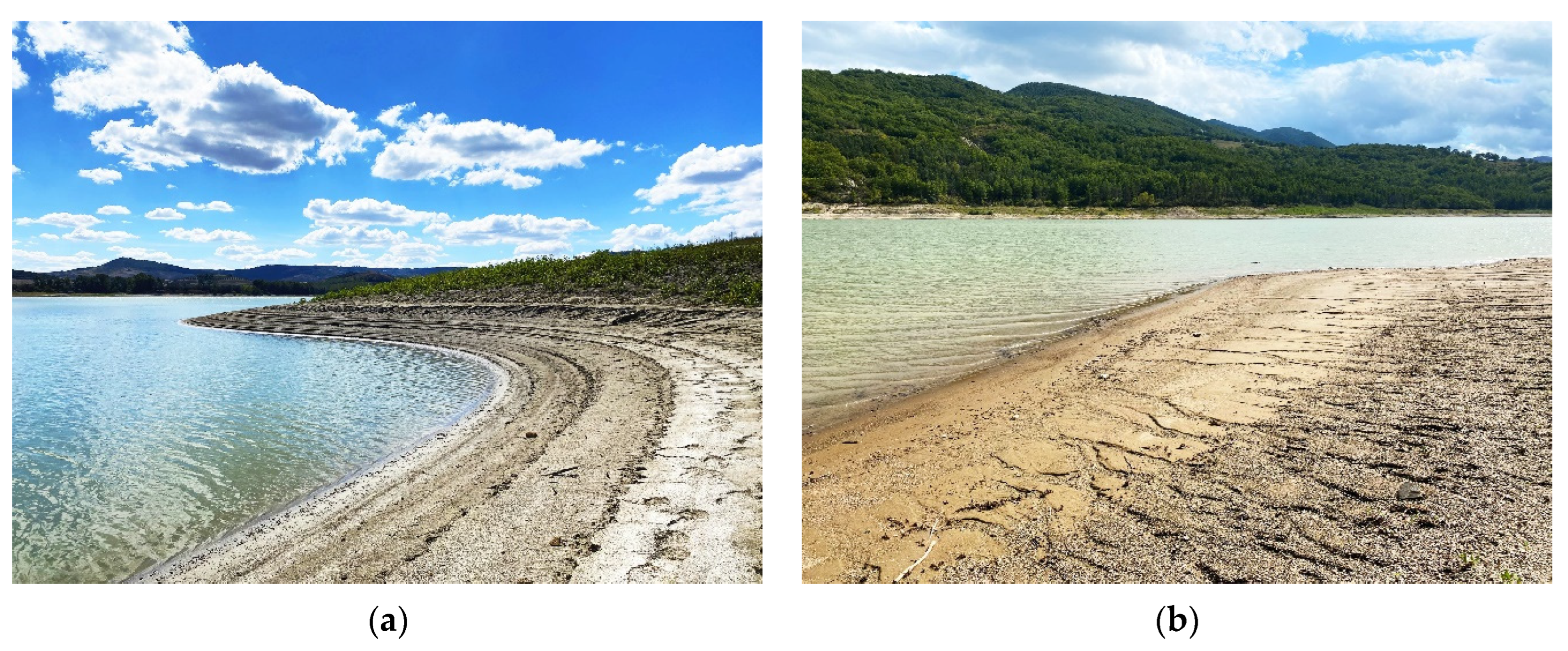
As shown in Martellotta et al., 2024 [67], the granulometric composition of the San Giuliano and Camastra reservoir sediments differs depending on the area from which the samples came. In fact, for both reservoirs, there is a predominance of the sandy component for sediments sampled near the dam and, on the contrary, a greater relevance of the silt-clay component in those coming from the upstream areas. The analyses relating to the organic component show that the organic matter content is greater for surface sediments from the Camastra reservoir than for those sampled from the banks of the San Giuliano reservoir. All sediments, however, have an organic matter content of less than 2%, so it can be considered negligible.

The samples SG_S5, SG_S6, SG_S8, and SG_S11 show the highest heavy metal content, corresponding to a predominant silt-clay grain size component and their position in the upstream areas of the reservoir. Regarding the organic matter content, sediment heavy metal concentration does not directly correlate with the measured values, except for sample SG_S5, for which the higher organic matter content corresponds to the higher heavy metal concentration.

Also, for the Camastra reservoir sediments, the most contaminated samples are located in the upstream areas, near the inlets of the Inferno and Camastra rivers, where the sediments are predominantly characterized by a clayey-silt matrix. In contrast to the San Giuliano sediments, for those in the Camastra, the sediments with the highest contaminant content are also those with the highest organic matter content.

Finally, it is noted that the variation in heavy metal content between all the samples is a direct consequence of the composition of the grain sizes of all the sediments analyzed within the same basin.

A comparison of the heavy metal contamination data in the sediments of the Camastra and the San Giuliano reservoirs with the data found for other reservoirs in the literature reveals that the Ni, Cu, and Zn concentrations are in line with the published parameters, in contrast to Pb, whose values found for the reservoirs examined are always significantly lower [68,69]. It has similar values to those determined for the surface sediments of Lake Taihu in China, except for samples SG_S5 and SG_S6 [70]. For Cr, on the other hand, the concentrations in the Camastra and San Giuliano sediments are always significantly lower than the corresponding values found for the Taihu Lake sediments, and are in line with those identified for Lake Symsar in Poland [71]. The extent of heavy metal contamination in the sediments of the investigated reservoirs is, therefore, not much more serious than in other similar studies.

3.2. Pollution Indices for Sediment Properties Evaluation

The sediment pollution evaluation, essential to defining its compatibility for reuse, was carried out by determining nine indices, which are made explicit in Section 2.4. Each of the indices was then compared with its respective threshold values to identify whether the sediments were polluted or not.

Table 13. Pollution indices estimated for sediments collected at the San Giuliano reservoir.

Pollution Indices	PN	PLI	Igeo	EF	PIavg	PIvector	PIN	MEC	RI
SG_S1	0.28	0.30	−0.18	1.16	0.38	0.63	4.13	0.28	9.83
SG_S2	0.13	0.08	−0.35	0.28	0.11	0.08	1.22	0.12	5.00
SG_S3	0.24	0.10	−0.30	0.39	0.16	0.22	1.77	0.21	9.03
SG_S4	0.25	0.19	−0.24	0.71	0.25	0.35	2.76	0.26	10.58
SG_S5	0.84	0.41	−0.12	1.68	0.63	2.99	28.77	0.80	33.49
SG_S6	0.48	0.31	−0.15	1.36	0.46	1.23	9.67	0.49	20.03
SG_S7	0.15	0.14	−0.26	0.61	0.20	0.19	2.18	0.18	6.84
SG_S8	0.31	0.30	−0.14	1.52	0.41	0.79	4.53	0.28	8.34
SG_S9	0.22	0.24	−0.18	1.21	0.33	0.48	3.64	0.25	8.01
SG_S10	0.17	0.19	−0.22	0.92	0.26	0.29	2.87	0.20	6.22
SG_S11	0.26	0.25	−0.17	1.29	0.35	0.54	3.82	0.26	8.14
SG_S12	0.09	0.11	−0.31	0.45	0.14	0.09	1.57	0.12	4.08

shows the pollution indices determined from the heavy metal shore surface distribution detected by sediment analysis of the San Giuliano reservoir. The shore surface sediments show a condition of absence of pollution or traces concerning most of the indices detected, although not for all. Three pollution indices (PN, PI_vector, and PIN) show the presence of contaminants or a low degree of pollution, with some differences. Nemerow’s pollution index indicates that only sample SG_S5 is characterized by a non-polluted condition, but at the limit (“warning limit”). On the other hand, the PI_vector and PIN indices report moderate pollutant content for only samples SG_S5 and SG_S6 (more evident and relevant for the former, less so for the latter). These sediment samples are the same ones for which As is reported to exceed the threshold value established by [31], thus highlighting how this heavy metal is the main factor responsible for the moderate pollution degree detected. Concerning the average values of all indices, however, the reservoir sediments appear not to be contaminated overall.

Table 14. Pollution indices estimated for sediments collected at the Camastra reservoir.

Pollution Indices	PN	PLI	Igeo	EF	PIavg	PIvector	PIN	MEC	RI
C_S1	0.17	0.22	−0.28	0.28	0.28	0.33	3.08	0.25	8.28
C_S2	0.24	0.28	−0.21	0.36	0.36	0.56	3.96	0.28	8.02
C_S3	0.49	0.41	−0.17	0.55	0.55	1.47	10.61	0.48	15.69
C_S4	0.47	0.38	−0.17	0.53	0.53	1.40	10.27	0.42	13.18
C_S5	0.28	0.31	−0.19	0.41	0.41	0.77	4.55	0.30	8.65
C_S6	0.24	0.26	−0.21	0.36	0.36	0.58	3.93	0.25	7.51
C_S7	0.23	0.27	−0.21	0.37	0.37	0.58	4.02	0.26	7.85
C_S8	0.42	0.36	−0.18	0.52	0.52	1.30	9.58	0.39	13.09
C_S9	0.51	0.39	−0.17	0.55	0.55	1.56	10.81	0.40	12.03
C_S10	0.32	0.32	−0.19	0.43	0.43	0.86	4.77	0.32	10.18
C_S11	0.45	0.37	−0.16	0.53	0.53	1.40	10.03	0.36	10.19
C_S12	0.22	0.25	−0.23	0.34	0.34	0.51	3.72	0.24	7.05
C_S13	0.24	0.25	−0.25	0.32	0.32	0.46	3.54	0.25	7.80

shows the values of the indices calculated for the Camastra reservoir shore surface sediments. It is noted that, for seven of the ten indices determined, the sediments show no polluted condition, identified as “clean” or “unpolluted,” and contamination can be defined as “low” or “absent.” The PI_vector and PIN indices, on the other hand, show that the Camastra sediments are characterized by a low content, or traces, of pollution, but only for the samples named C_S3, C_S4, C_S8, C_S9, and C_S11. Those are the specimens where Co exceeds the limit values; thus, it can be inferred that this heavy metal is responsible for the slight pollution condition identified. Moreover, the average value for each index is always below the thresholds above which sediments can be considered contaminated, even slightly.

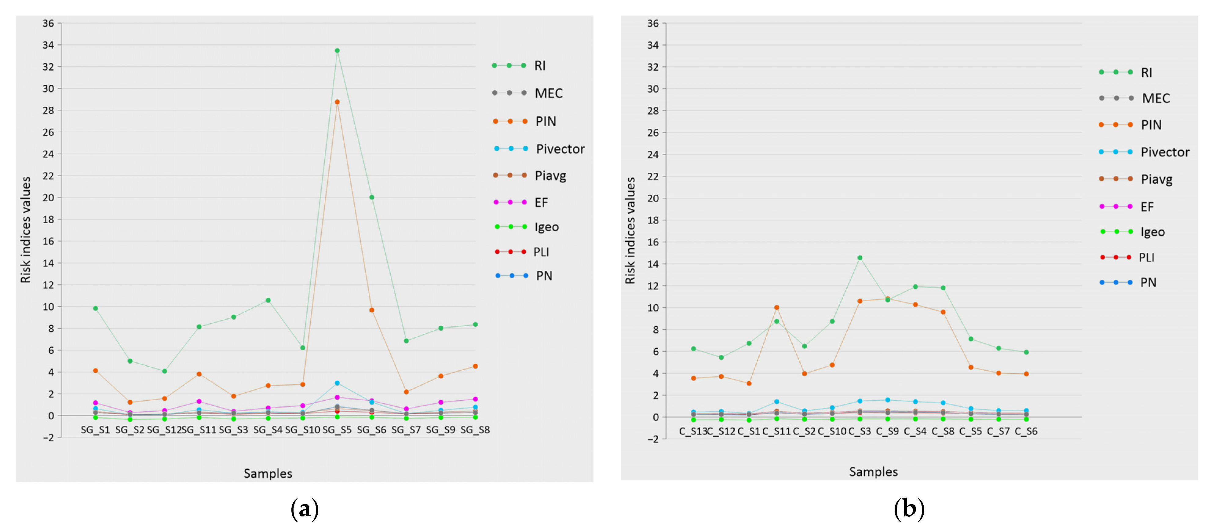
For both reservoirs, the highest values of the indices are associated with the Potential Ecological Risk (RI) index and the Background Enrichment Factor (PIN), even for the samples where the threshold concentration values are exceeded (Figure 5).

The values of the EF and MEC indices, which denote the possible pollution linked to anthropogenic activities, show that the exceedance found for As in the San Giuliano sediments and Co in the Camastra sediments is attributable neither to agronomic practices nor to the possible existence of industries but to the nature of the analyzed materials.

The spatial analysis of pollution indices as a function of the distance from the dam shows that the highest values are recorded for the sediments sampled at the central areas of both reservoirs’ banks, with no pollution in both upstream and downstream areas of the banks, where the pollution indices tend to be almost similar.

Examined indices for surface coastal sediments of the Camastra and the San Giuliano reservoirs are similar to those examined in other studies, both for sediments from reservoirs and for river sediments [38,42,52,68,69,70].

3.3. Multivariate Statistical Evaluation

3.3.1. Cluster Analysis

Cluster analysis (CA) was carried out to assess any similarities between sediments sampled in different areas of the reservoirs (spatial variability). For both the San Giuliano and the Camastra lakes, the assessments performed returned a dendrogram (Figure 6) in which all sampling sites, twelve for the San Giuliano and thirteen for the Camastra, were clustered into two statistically significant clusters, in both cases with a threshold of 60% (Height).

For the San Giuliano, the two clusters consist of sites SG_S2, SG_S3, SG_S4, SG_S7, and SG_S12, and sites SG_S1, SG_S5, SG_S6, SG_S8, SG_S9, SG_S10, and SG_S11, respectively. The two clusters obtained are heterogeneous, containing both upstream and downstream samples belonging to both reservoir banks, indicating that the pollution content is relatively uniform for the entire reservoir and that no peculiar elements significantly influence the pollutant content in sediments. Therefore, similar anthropogenic factors influence the heavy metal content in all samples. The main difference is in the heavy metal pollution content, where the cluster 1 group samples are characterized by a slight heavy metal concentration around the sampling sites, as opposed to the higher contamination level at the sampling sites belonging to cluster 2.

Regarding the Camastra reservoir, the two clusters identified reflect the spatial distribution of sampling sites. The cluster 1 group samples C_S3, C_S4, C_S8, C_S9, C_S10, and C_S11 all belong to the central area of the reservoir; cluster 2, on the other hand, contains samples C_S1, C_S2, C_S5, C_S6, C_S12, and C_S13, located in the downstream and upstream zones. The different pollution levels of specimens, whose probable sources will be discussed in the next section, therefore depend on the location of the sampling sites. The main difference between the areas related to the identified clusters lies in the presence of mobility infrastructure (roads, bridges, etc.) in the upstream and downstream areas, although with limited traffic concentration, in contrast to the central area.

3.3.2. Correlation Matrix

Table 15. Pollutants correlation matrix in the San Giuliano specimens.

	As	Be	Co	Cr	Cu	Ni	Pb	Sb	Tl	V	Zn
As	1
Be	-	1
Co	-	0.696 a,*	1
Cr	-	0.959 a,**	0.812 a,**	1
Cu	-	0.904 a,**	0.893 a,**	0.938 a,**	1
Ni	-	0.862 a,**	0.932 a,**	0.951 a,**	0.937 a,**	1
Pb	-	0.634 a,*	0.969 a,**	0.722 a,**	0.868 a,**	0.858 a,**	1
Sb	0.758 b,**	-	-	-	-	-	-	1
Tl	0.016 b	-	-	-	-	-	-	0.078 b	1
V	-	0.939 a,**	0.818 a,**	0.942 a,**	0.926 a,**	0.903 a,**	0.776 a,**	-	-	1
Zn	-	0.979 a,**	0.687 a,*	0.945 a,*	0.919 a,**	0.833 a,**	0.633 a,*	-	-	0.935 a,**	1

Notes: Bold values (Pearson’s r coefficient or Kendall’s τ coefficient) show significant correlation. ^a Pearson’s r coefficient for heavy metal values with a normal distribution. ^b Kendall’s τ coefficient for heavy metal values with a non-normal distribution. * significance at the 0.05 probability level (p-value < 0.05). ** significance at the 0.01 probability level (p-value < 0.01).

and

Table 16. Pollutants correlation matrix in the Camastra specimens.

	As	Be	Co	Cr	Cu	Ni	Pb	Sb	Tl	V	Zn
As	1
Be	-	1
Co	0.441 b,**	-	1
Cr	-	0.742 a,**	-	1
Cu	-	0.798 a,**	-	0.598 a,*	1
Ni	-	0.580 a,*	-	0.522 a,*	0.777 a,**	1
Pb	0.518 b,**	-	0.750 b,**	-	-	-	1
Sb	-	0.206 a	-	0.171 a	0.412 a	0.815 a,**	-	1
Tl	-	0.634 a,**	-	0.664 a,**	0.302 a	0.068 a	-	−0.285 a	1
V	-	0.817 a,**	-	0.956 a,**	0.577 a,*	0.439 a	-	0.061 a	0.682 a,**	1
Zn	-	0.889 a,**	-	0.566 a,*	0.888 a,**	0.693 a,**	-	0.445 a	0.304 a	0.611 a,**	1

Notes: Bold values (Pearson’s r coefficient or Kendall’s τ coefficient) show significant correlation. ^a Pearson’s r coefficient for heavy metal values with a normal distribution. ^b Kendall’s τ coefficient for heavy metal values with a non-normal distribution. * significance at the 0.05 probability level (p-value < 0.05). ** significance at the 0.01 probability level (p-value < 0.01).

show the correlation matrices of the heavy metals detected in the San Giuliano and Camastra sediments to determine the common pollution sources in the samples. For heavy metals whose samples have a normal distribution, the values of Pearson’s correlation coefficient are given; if the data distribution does not follow the Gaussian curve, the table contains the value of Kendall’s τ coefficient.

For the San Giuliano reservoir, there is a significant positive correlation between some of the heavy metals studied. Pearson’s coefficient values are close to unity, with a p-value of less than 0.01, and are found for several parameters. Be is significantly correlated with Cr, Cu, V, and Zn; Co shows a significant relationship with Ni and Pb. In addition, a relevant correlation is also recorded between Cr, Cu, Ni, V, and Zn, indicating that these elements probably originated from the same source. Regarding the correlation between heavy metals whose data do not follow a normal distribution, Kendall’s τ coefficient values show an important significance degree between As and Sb, with a p-value < 0.01.

For all other heavy metals, the correlations are negative or, at any rate, insignificant, indicating relatively complex pollution sources.

3.4. Ecological Risk Assessment

To assess the potential ecological risk associated with the shore surface distribution of pollutants in sediments sampled at the Camastra and San Giuliano lakes’ banks, the RI index, described in Section 2.4.9, was evaluated [72]. Table 9 and Table 10 show that the contaminant medium values in the investigated shore surface sediments for the calculation of this index (As, Cr, Cu, Ni, Pb, Zn) are, for both reservoirs, consistently lower than the concentration threshold values set by current Italian standards. In addition, values are higher than the toxicity response in the latter case, except for the As value for the Camastra reservoir. Specifically, for the Camastra reservoir, the values of Cr, Cu, Ni, Pb, and Zn are about 30 times, 6 times, 9 times, 3 times, and 42 times higher than the related toxicity response value, respectively; on the contrary, the concentration of As is 70% of the value reported in Table 7. Regarding the San Giuliano reservoir, however, it is found that the concentrations of As, Cr, Cu, Ni, Pb, and Zn are about 1.5 times, 19 times, 3 times, 6.5 times, 2 times, and 22 times higher than the related toxicity response value, indicating that these heavy metals could partly come from contamination sources outside the reservoir [73].

Figure 5 shows, among all indices, that RI ranges from a minimum of 4.08 to a maximum of 33.49 for the San Giuliano reservoir shore surface sediments and from a minimum of 7.05 to a maximum of 15.69 for the Camastra reservoir coastal shore surface sediments. Considering the categories for RI value shown in Table 8, all samples are classified with “low” pollution risk. The distribution of RI values for the San Giuliano reservoir (Figure 5a) almost overlaps with the PIN index and the Camastra reservoir (Figure 5b). Furthermore, for both reservoirs, it is shown that the potential ecological risk of the upstream areas is, on average, higher than that of the downstream areas. Since the potential ecological risk index defines the level of potential risk associated with the presence of pollutants in a certain environment, this study’s results indicate that the areas more susceptible to pollution risk are, for both reservoirs, those upstream, whose lithogenic composition is such that the sediments are potentially less employable.

Finally, for the San Giuliano reservoir, the RI index appears to be highest for samples SG_S5 and SG_S6; in contrast, sediments sampled at the Camastra reservoir banks take the highest value at sites C_S3, C_S4, C_S8, and C_S9. Since the sites mentioned before are the same for which exceedances occurred for As in the San Giuliano sediments and Co in the Camastra sediments, respectively, it is evident that the peak RI value shown in the trends is closely related to and influenced by these heavy metals.

3.5. Metal Pollution Sources

The analyses carried out up to this point, especially the statistical evaluations, were focused on assessing the shore distribution of pollutants for the sampled at surface sediments and, once this was defined, evaluating the possible sources influencing the concentration of heavy metals, according to the procedure in Duodu et al., 2016 [37]. The shore surface sediments of the two reservoirs considered, with different geology, lithology, land use, anthropization, and, more generally, characteristics, show significantly different parameters, facilitating the assessments carried out in this section.

Regarding the exceedance of the concentration threshold value for As at the San Giuliano reservoir, the two shore surface samples (SG_S5 and SG_S6) were spatially close and grouped in the same cluster, so the pollution sources are multiple. The analysis of the geology of the area, both the San Giuliano basin and the catchment areas of the lateral tributaries, shows the predominance of alluvial deposits that contain organic substance, determining the concentration of metals and results in the accumulation of arsenic in the sediments, where it reaches due to the transport by the tributary streams. In addition, the peat that characterizes the surface layer of the soil typically shows a conspicuous As content. An additional factor influencing the higher value of this heavy metal in the shore surface sediments is algal organic matter reaching the lake environment, also introduced by the lateral, temporary, and permanent tributaries. The influence of the organic matter is confirmed by the value above the thresholds of some pollution indices and by what is shown in Table 13 and Table 14, since its accumulation even increases other metals (in the present case, antimony). In addition, further As sources are the sedimentary rocks, where it is usually significant, and the reducing environment that characterizes the upstream area of the lake, as evidenced by the specimen’s dark grey colour; these avoid the transition from oxidation state V to oxidation state III, are much more soluble and, therefore, are more prone to leaching.

Concerning the regulatory limits exceedance for Co in the Camastra shore surface sediments, the primary source of this heavy metal is the ultra-basic magmatic rocks, which concentrate iron–magnesium minerals, in which cobalt tends to accumulate, prevalent within the watershed of the Inferno and Camastra rivers, and their lateral tributaries, which feed the reservoir. In addition, the geological composition of the upstream areas even points to the presence of sedimentary rocks, in which cobalt is also concentrated, as well as in soil with organic matter.

In both reservoirs, Pearson’s correlation test shows a significant correlation between V and Cr, suggesting that the contamination of coastal shore surface sediments is due to anthropogenic input, related to leached ground discharges from rainfall falling into the Camastra reservoir and deriving from the lateral tributaries’ contribution. Ni and Zn also have a significant correlation for both reservoirs, indicating phenomena of diesel and lubricating oil combustion and tire and brake abrasion. This is explained by the accessibility of the reservoir areas by motor vehicles, which can arrive undisturbed within a few meters of the areas where the samples were taken. The further correlation found for both parameters with Cu denotes the presence of iron structures, e.g., the management and regulation organs of the dams, treated with antifouling paints. In addition, the significant correlation between As and Sb for the San Giuliano reservoir suggests a common pollutant source from the mining and smelting of antimony ores.

Finally, the low values found for the EF and MEC indices indicate that the coastal distribution of pollutants is not associated with the presence of industries, which cannot be detected in the areas close to both reservoirs. For this reason, we can assume that the values found relate to the type of rocks that characterize the areas linked to lakes and lithogenic sources.

To improve the sediment quality and limit coastal pollution, various initiatives could be started. In this sense, the improvement could take place through three main actions: the removal of sediment and recycling, the admission of unpolluted water, and the limitation of watershed erosion.

4. Conclusions

The reservoir dredging activities result in the need to manage large quantities of sediment currently labeled as waste and, therefore, disposed of in landfills, with very high environmental costs. In this scenario, it is necessary to identify alternatives for reusing these materials, so sediment characterization activities are crucial, especially those concerning heavy metals.

This research verified that specimens collected at the San Giuliano and Camastra lakes do not exceed the considered contamination threshold values, except for As in two samples of the San Giuliano reservoir and Co in five samples of the Camastra reservoir. The analysis of the contaminants’ spatial distribution highlights that the San Giuliano reservoir’s upstream areas and the Camastra reservoir’s central areas record the highest heavy metal concentrations.

An analysis of the observed results highlights the following main points concerning pollution risk assessment:

• Absence of pollution in almost all samples;
• Higher contamination degree in the central areas of the Camastra reservoir;
• Risk conditions only regarding As for the San Giuliano Lake and Co for the Camastra Lake, even if the average contamination values for the two areas show a limited or no pollution condition;
• The same potential pollution sources exist for both reservoirs due to the geological composition of the related areas.

Therefore, following the analyses, the San Giuliano and the Camastra reservoirs’ sediments lend themselves to potential reuse in various application fields, significantly reducing landfill disposal and, consequently, the associated environmental costs. In this sense, the authors suggest the following possible reuses:

• Construction field, as building materials for the fine part of the sediment, incorporating them into mortars or even replacing part of the sand or cement [74,75,76,77];
• Agriculture, to reconstitute soils;
• Reuse of the coarse part directly as fill or backfill material.

The coarse part can be reused.

In any case, if it is deemed that sediments from both reservoirs where the heavy metal value exceeds the corresponding regulatory limit are unsuitable for the intended reuse, the areas where the limit values are exceeded could be isolated, and only those where there is an absence of contamination could be reused. In this regard, only a tiny percentage of the sampled sediment would be landfilled, thus limiting environmental impacts and ensuring the availability of secondary raw material to replace the current virgin materials, an additional benefit the proposal in this study would achieve.

References

1. Biemans, H.; Haddeland, I.; Kabat, P.; Ludwig, F.; Hutjes, R.W.A.; Heinke, J.; von Bloh, W.; Gerten, D. Impact of reservoirs on river discharge and irrigation water supply during the 20th century. Water Resour. Res. 2011, 47. [Google Scholar] [CrossRef]
2. Lu, Y.; Zeng, Y.; Wang, W. Relation disentanglement, the potential risk assessment, and source identification of heavy metals in the sediment of the Changzhao Reservoir, Zhejiang Province. Environ. Sci. Pollut. Res. 2023, 30, 82625–82636. [Google Scholar] [CrossRef] [PubMed]
3. Niu, Y.; Shah, F.A. Economics of optimal reservoir capacity determination, sediment management, and dam decommissioning. Water Resour. Res. 2021, 57, e2020WR028198. [Google Scholar] [CrossRef]
4. Canlı, O.; Çetintürk, K.; Güzel, B. A comprehensive assessment, source input determination and distribution of persistent organic pollutants (POPs) along with heavy metals (HMs) in reservoir lake sediments from Çanakkale province, Türkiye. Environ. Geochem. Health 2023, 45, 3985–4006. [Google Scholar] [CrossRef]
5. Rovira, A.; Ibàñez, C. Sediment management options for the lower Ebro River and its delta. J. Soils Sediments 2007, 7, 285–295. [Google Scholar] [CrossRef]
6. Kondolf, G.M.; Gao, Y.; Annandale, G.W.; Morris, G.L.; Jiang, E.; Zhang, J.; Cao, Y.; Carling, P.; Fu, K.; Guo, Q.; et al. Sustainable sediment management in reservoirs and regulated rivers: Experiences from five continents. Earth’s Future 2014, 2, 256–280. [Google Scholar] [CrossRef]
7. Cimorelli, L.; Covelli, C.; De Vincenzo, A.; Pianese, D.; Molino, B. Sedimentation in reservoirs: Evaluation of return periods related to operational failures of water supply reservoirs with Monte Carlo simulation. J. Water Resour. Plan. Manag. 2021, 147, 04020096. [Google Scholar] [CrossRef]
8. Mirauda, D.; Pannone, M.; De Vincenzo, A. An entropic model for the assessment of streamwise velocity dip in wide open channels. Entropy 2018, 20, 69. [Google Scholar] [CrossRef]
9. Covelli, C.; Cimorelli, L.; Pagliuca, D.N.; Molino, B.; Pianese, D. Assessment of erosion in river basins: A distributed model to estimate the sediment production over watersheds by a 3-dimensional LS factor in RUSLE model. Hydrology 2020, 7, 13. [Google Scholar] [CrossRef]
10. Palmieri, A.; Shah, F.; Dinar, A. Economics of reservoir sedimentation and sustainable management of dams. J. Environ. Manag. 2001, 61, 149–163. [Google Scholar] [CrossRef]
11. Djeran-Maigre, I.; Razakamanantsoa, A.; Levacher, D.; Hussain, M.; Delfosse, E. A relevant characterization of Usumacinta river sediments for a reuse in earthen construction and agriculture. J. S. Am. Earth Sci. 2023, 125, 104317. [Google Scholar] [CrossRef]
12. Bortali, M.; Rabouli, M.; Yessari, M.; Hajjaji, A. Characterizing harbor dredged sediment for sustainable reuse as construction material. Sustainability 2023, 15, 1834. [Google Scholar] [CrossRef]
13. Cheng, N.; Liu, L.; Hou, Z.; Wu, J.; Wang, Q.; Fu, Y. Pollution characteristics and risk assessment of surface sediments in the urban lakes. Environ. Sci. Pollut. Res. Int. 2021, 17, 22022–22037. [Google Scholar] [CrossRef] [PubMed]
14. Geng, M.; Qian, Z.; Jiang, H.; Huang, B.; Huang, S.; Deng, B.; Peng, Y.; Xie, Y.; Li, F.; Zou, Y.; et al. Assessing the impact of water-sediment factors on water quality to guide river-connected lake water environment improvement. Sci. Total Environ. 2024, 912, 168866. [Google Scholar] [CrossRef]
15. Chiaia-Hernández, A.C.; Casado-Martinez, C.; Lara-Martin, P.; Bucheli, T.D. Sediments: Sink, archive, and source of contaminants. Environ. Sci. Pollut. Res. 2022, 29, 85761–85765. [Google Scholar] [CrossRef]
16. Li, G.; Chen, R.; Li, Z.; Wu, X.; Xiang, K.; Wang, C.; Peng, Y. Ecological Risk and Human Health Assessment of Heavy Metals in Sediments of Datong Lake. Toxics 2025, 13, 560. [Google Scholar] [CrossRef]
17. Gouré-Doubi, H.; Lecomte-Nana, G.; Thery, F.; Peyratout, C.; Anger, B.; Levacher, D. Characterization and valorization of dam sediment as ceramic materials. Int. J. Eng. Innov. Technol. 2015, 4, 84–91. [Google Scholar]
18. Haurine, F.; Cojan, I.; Bruneaux, M.A. Development of an industrial mineralogical framework to evaluate mixtures from reservoir sediments for recovery by the heavy clay industry: Application of the Durance system (France). Appl. Clay Sci. 2016, 132, 508–517. [Google Scholar] [CrossRef]
19. Faure, A.; Coudray, C.; Anger, B.; Moulin, I.; Colina, H.; Izoret, L.; Théry, F.; Smith, A. Beneficial reuse of dam fine sediments as clinker raw material. Constr. Build. Mater. 2019, 218, 365–384. [Google Scholar] [CrossRef]
20. Mesrar, L.; Benamar, A.; Duchemin, B.; Brasselet, S.; Bourdin, F.; Jabrane, R. Engineering properties of dredged sediments as a raw resource for fired bricks. Bull. Eng. Geol. Environ. 2021, 80, 2643–2658. [Google Scholar] [CrossRef]
21. Chahal, H.; Pothier, C.; Djeran-Maigre, I. Study of landfills using GCL for PCB contaminated sediments. In Proceedings of the 5th European Geosynthetics Congress, Valencia, Spain, 16–19 September 2012. [Google Scholar]
22. Kutlu, B. Contamination and ecological risk assessment of heavy metals in surface sediments of the Munzur stream, Turkey. Pol. J. Environ. Stud. 2023, 32, 587–597. [Google Scholar] [CrossRef] [PubMed]
23. Li, X.; Bing, J.; Zhang, J.; Guo, L.; Deng, Z.; Wang, D.; Liu, L. Ecological risk assessment and sources identification of heavy metals in surface sediments of a river–reservoir system. Sci. Total Environ. 2022, 842, 156683. [Google Scholar] [CrossRef]
24. Proshad, R.; Kormoker, T.; Al, M.A.; Islam, M.S.; Khadka, S.; Idris, A.M. Receptor model-based source apportionment and ecological risk of metals in sediments of an urban river in Bangladesh. J. Hazard. Mater. 2022, 423, 127030. [Google Scholar] [CrossRef] [PubMed]
25. Wu, W.; Qu, S.; Nel, W.; Ji, J. Tracing and quantifying the sources of heavy metals in the upper and middle reaches of the Pearl River Basin: New insights from Sr-Nd-Pb multi-isotopic systems. Chemosphere 2022, 288, 132630. [Google Scholar] [PubMed]
26. Muller, G. Index of geoaccumulation in sediments of the Rhine River. Geol. J. 1969, 2, 109–118. [Google Scholar]
27. Tomlinson, D.L.; Wilson, J.G.; Harris, C.R.; Jeffrey, D.W. Problems in the assessment of heavy-metal levels in estuaries and the formation of a pollution index. Helgoländer Meeresunters. 1980, 33, 566–575. [Google Scholar] [CrossRef]
28. Gong, Q.; Deng, J.; Xiang, Y.; Wang, Q.; Yang, L. Calculating pollution indices by heavy metals in ecological geochemistry assessment and a case study in parks of Beijing. J. China Univ. Geosci. 2008, 19, 230–241. [Google Scholar]
29. Brady, J.P.; Ayoko, G.A.; Martens, W.N.; Goonetilleke, A. Enrichment, distribution and sources of heavy metals in the sediments of Deception Bay, Queensland, Australia. Mar. Pollut. Bull. 2014, 81, 248–255. [Google Scholar]
30. Vidal, D.E.; Bay, S.M. Comparative sediment quality guideline performance for predicting sediment toxicity in southern California, USA. Environ. Toxicol. Chem. 2005, 24, 3173–3182. [Google Scholar] [CrossRef]
31. Italian Decree n. 120/2017. Available online: https://www.gazzettaufficiale.it/eli/id/2017/08/07/17G00135/sg (accessed on 22 March 2025).
32. Terzi, M.H.; Kalkan, M. Evaluation of soil pollution by heavy metal using index calculations and multivariate statistical analysis. Environ. Monit. Assess. 2024, 196, 443. [Google Scholar] [CrossRef]
33. Zhang, T.; Wang, M.; Bai, G.; Liu, J.; Li, P.; Zhang, Y.; Xia, S. Distribution characteristics, risk assessment, and source analysis of heavy metals in surface sediments and near-lakeshore soils of a plateau lake in China. Gondwana Res. 2023, 115, 191–200. [Google Scholar] [CrossRef]
34. Izah, S.C.; Richard, G.; Aigberua, A.O.; Ekakitie, O. Variations in reference values utilized for the evaluation of complex pollution indices of potentially toxic elements: A critical review. Environ. Chall. 2021, 5, 100322. [Google Scholar] [CrossRef]
35. Enjavinejad, S.M.; Zahedifar, M.; Moosavi, A.A.; Khosravani, P. Integrated application of multiple indicators and geographic information system-based approaches for comprehensive assessment of environmental impacts of toxic metals-contaminated agricultural soils and vegetables. Sci. Total Environ. 2024, 926, 171747. [Google Scholar] [CrossRef]
36. Hamzenejhad, R. Quantitative assessment of soil heavy metals pollution. Appl. Soil Res. 2020, 8, 37–52. [Google Scholar]
37. Duodu, G.O.; Goonetilleke, A.; Ayoko, G.A. Comparison of pollution indices for the assessment of heavy metal in Brisbane River sediment. Environ. Pollut. 2016, 219, 1077–1091. [Google Scholar] [CrossRef] [PubMed]
38. Ferreira, S.L.C.; da Silva Junior, J.B.; dos Santos, I.F.; de Oliveira, O.M.C.; Cerda, V.; Queiroz, A.F. Use of pollution indices and ecological risk in the assessment of contamination from chemical elements in soils and sediments–Practical aspects. Trends Environ. Anal. Chem. 2022, 35, e00169. [Google Scholar] [CrossRef]
39. Baran, A.; Tack, F.M.G.; Delemazure, A.; Wieczorek, J.; Tarnawski, M.; Birch, G. Metal contamination in sediments of dam reservoirs: A multi-facetted generic risk assessment. Chemosphere 2023, 310, 136760. [Google Scholar] [CrossRef]
40. Liu, Y.; Zhou, Z.; Gong, W.; Xu, Y.; Ding, Q.; Cui, L. Distribution, risk assessment of heavy metals in sediments, and their potential risk on water supply safety of a drinking water reservoir, middle China. Environ. Sci. Pollut. Res. 2023, 30, 73702–73713. [Google Scholar] [CrossRef]
41. Liu, S.; Yu, F.; Lang, T.; Ji, Y.; Fu, Y.; Zhang, J.; Ge, C. Spatial distribution of heavy metal contaminants: The effects of water-sediment regulation in the Henan section of the Yellow River. Sci. Total Environ. 2023, 892, 164568. [Google Scholar] [CrossRef]
42. Liang, R.Z.; Gu, Y.G.; Li, H.S.; Han, Y.J.; Niu, J.; Su, H.; Jordan, R.W.; Man, X.T.; Jiang, S.J. Multi-index assessment of heavy metal contamination in surface sediments of the Pearl River estuary intertidal zone. Mar. Pollut. Bull. 2023, 186, 114445. [Google Scholar] [CrossRef]
43. Wang, W.; Wu, F.; Yin, T.; Jiang, S.; Tang, S. Distribution, source, and contamination assessment of heavy metals in surface sediments of the Zhifu Bay in northern China. Mar. Pollut. Bull. 2023, 194, 115449. [Google Scholar] [CrossRef]
44. ISO 17402:2008; Soil Quality—Requirements and Guidance for the Selection and Application of Methods for the Assessment of Bioavailability of Contaminants in Soil and Soil Materials. International Organization for Standardization (ISO): Geneva, Switzerland, 2008. Available online: https://www.iso.org/standard/38349.html (accessed on 15 March 2025).
45. EPA standard 3051A; Microwave Assisted acid Digestion of Sediments, Sludges, Soils, and Oils. Environmental Protection Agency (EPA): Washington, DC, USA, 2007. Available online: https://www.epa.gov/sites/default/files/2015-12/documents/3051a.pdf (accessed on 15 March 2025).
46. Islam, M.S.; Shammi, R.S.; Jannat, R.; Kabir, M.H.; Islam, M.S. Spatial distribution and ecological risk of heavy metal in surface sediment of Old Brahmaputra River, Bangladesh. Chem. Ecol. 2023, 39, 173–201. [Google Scholar] [CrossRef]
47. UNI EN ISO 9001:2015; Quality Management Systems—Requirements. Italian Organization for Standardization (UNI): Milan, Italy, 2015. Available online: https://store.uni.com/uni-en-iso-9001-2015-a1-2024 (accessed on 15 March 2025).
48. UNI EN ISO 17025:2018; General Requirements for the Competence of Testing and Calibration Laboratories. Italian Organization for Standardization (UNI): Milan, Italy, 2018. Available online: https://store.uni.com/uni-cei-en-iso-iec-17025-2018 (accessed on 15 March 2025).
49. Kowalska, J.B.; Mazurek, R.; Gąsiorek, M.; Zaleski, T. Pollution indices as useful tools for the comprehensive evaluation of the degree of soil contamination–A review. Environ. Geochem. Health 2018, 40, 2395–2420. [Google Scholar] [CrossRef] [PubMed]
50. Ahirvar, B.P.; Das, P.; Srivastava, V.; Kumar, M. Perspectives of heavy metal pollution indices for soil, sediment, and water pollution evaluation: An insight. Total Environ. Res. Themes 2023, 6, 100039. [Google Scholar] [CrossRef]
51. Varol, M. Assessment of heavy metal contamination in sediments of the Tigris River (Turkey) using pollution indices and multivariate statistical techniques. J. Hazard. Mater. 2011, 195, 355–364. [Google Scholar] [CrossRef]
52. Barbieri, M. The importance of enrichment factor (EF) and geoaccumulation index (Igeo) to evaluate the soil contamination. J. Geol. Geophys. 2016, 5, 1–4. [Google Scholar] [CrossRef]
53. Chen, T.-B.; Zheng, Y.-M.; Lei, M.; Huang, Z.-C.; Wu, H.-T.; Chen, H.; Fan, K.-K.; Yu, K.; Wu, X.; Tian, Q.-Z. Assessment of heavy metal pollution in surface soils of urban parks in Beijing, China. Chemosphere 2005, 60, 542–551. [Google Scholar] [CrossRef]
54. Sakan, S.M.; Đorđević, D.S.; Manojlović, D.D.; Predrag, P.S. Assessment of heavy metal pollutants accumulation in the Tisza river sediments. J. Environ. Manag. 2009, 90, 3382–3390. [Google Scholar] [CrossRef]
55. Sucharovà, J.; Suchara, I.; Hola, M.; Marikova, S.; Reimann, C.; Boyd, R.; Filzmoser, P.; Englmaier, P. Top-/bottom-soil ratios and enrichment factors: What do they really show? Appl. Geochem. 2012, 27, 138–145. [Google Scholar] [CrossRef]
56. Bhuiyan, M.A.; Parvez, L.; Islam, M.A.; Dampare, S.B.; Suzuki, S. Heavy metal pollution of coal mine-affected agricultural soils in the northern part of Bangladesh. J. Hazard. Mater. 2010, 173, 384–392. [Google Scholar] [CrossRef]
57. Kloke, A. Contents of Arsenic, Cadmium, Chromium, Fluorine, Lead, Mercury and Nickel in Plants Grown on Contaminated soil. In Proceedings of the UN-ECE Symposium, Geneva, Switzerland, 7 August 1979. [Google Scholar]
58. Chen, H.; Chen, Z.; Chen, Z.; Ou, X.; Chen, J. Calculation of Toxicity Coefficient of Potential Ecological Risk Assessment of Rare Earth Elements. Bull. Environ. Contam. Toxicol. 2020, 104, 582–587. [Google Scholar] [CrossRef] [PubMed]
59. Li, Q.; Chen, M.; Zheng, X.; Chen, W. Determination of tungsten’s toxicity coefficient for potential ecological risk assessment. Environ. Res. Commun. 2023, 5, 025003. [Google Scholar] [CrossRef]
60. Simeonov, V.; Einax, J.; Tsakovski, S.; Kraft, J. Multivariate statistical assessment of polluted soils. Open Chem. 2005, 3, 1–9. [Google Scholar] [CrossRef]
61. Shapiro, S.S.; Wilk, M.B. An analysis of variance test for normality (complete samples). Biometrika 1965, 52, 591–611. [Google Scholar] [CrossRef]
62. Royston, P. Approximating the Shapiro-Wilk W-test for non-normality. Stat. Comput. 1992, 2, 117–119. [Google Scholar] [CrossRef]
63. Hanusz, Z.; Tarasinska, J.; Zielinski, W. Shapiro-Wilk test with known mean. Revstat Stat. J. 2016, 14, 89–100. [Google Scholar] [CrossRef]
64. Kendall, M.G. A new measure of rank correlation. Biometrika 1938, 30, 81–93. [Google Scholar] [CrossRef]
65. Akoto, O.; Yakubu, S.; Ofori, L.A.; Bortey-Sam, N.; Boadi, N.O.; Horgah, J.; Sackey, L.N. Multivariate studies and heavy metal pollution in soil from gold mining area. Heliyon 2023, 9, e12661. [Google Scholar] [CrossRef]
66. Italian Decree n. 152/2006. Available online: https://www.gazzettaufficiale.it/dettaglio/codici/materiaAmbientale (accessed on 18 March 2025).
67. Martellotta, A.M.N.; Levacher, D.; Gentile, F.; Ranieri, G.; Trabace, T.; Piccinni, A.F. A Relevant Characterization and Compatibility for Reuse the Sediments from Reservoirs in Southern Italy. Appl. Sci. 2024, 14, 727. [Google Scholar] [CrossRef]
68. Guo, W.; Huo, S.; Xi, B.; Zhang, J.; Wu, F. Heavy metal contamination in sediments from typical lakes in the five geographic regions of China: Distribution, bioavailability, and risk. Ecol. Eng. 2015, 81, 243–255. [Google Scholar] [CrossRef]
69. Xu, Y.; Wu, Y.; Han, J.; Li, P. The current status of heavy metal in lake sediments from China: Pollution and ecological risk assessment. Ecol. Evol. 2017, 7, 5454–5466. [Google Scholar] [CrossRef] [PubMed]
70. Niu, Y.; Jiang, X.; Wang, K.; Xia, J.; Jiao, W.; Niu, Y.; Yu, H. Meta analysis of heavy metal pollution and sources in surface sediments of Lake Taihu, China. Sci. Total Environ. 2020, 700, 134509. [Google Scholar] [CrossRef] [PubMed]
71. Kuriata-Potasznik, A.; Szymczyk, S.; Skwierawski, A.; Glińska-Lewczuk, K.; Cymes, I. Heavy metal contamination in the surface layer of bottom sediments in a flow-through lake: A case study of Lake Symsar in Northern Poland. Water 2016, 8, 358. [Google Scholar] [CrossRef]
72. Zhang, Z.; Lu, Y.; Li, H.; Tu, Y.; Liu, B.; Yang, Z. Assessment of heavy metal contamination, distribution and source identification in the sediments from the Zijiang River, China. Sci. Total Environ. 2018, 645, 235–243. [Google Scholar] [CrossRef] [PubMed]
73. Ye, J.-H.; Yu, T.; Xu, Z.-T.; Liu, H.-Y.; Cai, Q.-R. Distribution and probabilistic integrated ecological risk assessment of heavy metals in the surface water of Poyang Lake, China. Chin. J. Anal. Chem. 2021, 49, 29–34. [Google Scholar] [CrossRef]
74. Junakova, N.; Junak, J. Recycling of reservoir sediment material as a binder in concrete. Procedia Eng. 2017, 180, 1292–1297. [Google Scholar] [CrossRef]
75. Anger, B.; Levacher, D.; Théry, F. A minimal characterization identification approach for pre-selecting dam fine sediments reuse options. In Proceedings of the 8th International SedNet Conference, Lisbon, Portugal, 6–9 November 2013; Available online: https://sednet.org/download/2013-poster9-Anger-et-al.pdf (accessed on 4 July 2023).
76. Valenti, G.; Bernardo, G.; Marroccoli, M.; Molino, B. Beneficial reuse of reservoir sediment in the cement industry. In Proceedings of the 2nd International Conference on the Remediation of Contaminated Sediments, Venice, Italy, 30 September–3 October 2003; Available online: https://hdl.handle.net/11695/14474 (accessed on 7 July 2023).
77. Rozière, E.; Samara, M.; Loukili, A.; Damidot, D. Valorisation of sediments in self-consolidating concrete: Mix-design and microstructure. Constr. Build. Mater. 2015, 81, 1–10. [Google Scholar] [CrossRef]
Figure 1. Map of the San Giuliano (a) and Camastra (b) reservoirs and the sampling sites (red points).
Water 17 02042 g001
Figure 2. Rainfall trends for the two lakes in the sampling years (the dotted lines represents the average rainfall values for each reservoirs).
Water 17 02042 g002
Figure 3. Sediments sampled at the hydraulic left bank of the San Giuliano (a) and the Camastra (b) lakes.
Water 17 02042 g003
Figure 4. Heavy metal values detected in deposits collected at the San Giuliano (a) and Camastra (b) lakes, ordered as distance from the dam increases.
Water 17 02042 g004
Figure 5. Pollution indices for samples taken at the San Giuliano (a) and Camastra (b) reservoirs, ordered as distance from the dam increases.
Water 17 02042 g005
Figure 6. Dendrogram highlighting the clustering of the sampling sites of the San Giuliano (a) and the Camastra (b) reservoir (* indicates the significance at the 0.05 probability level).
Water 17 02042 g006