Flood Susceptibility Assessment Using Multi-Tier Feature Selection and Ensemble Boosting Machine Learning Models

Abstract

Flood susceptibility modeling (FSM) plays a key role in advancing proactive disaster risk reduction and spatial planning. This research developed FSM for the Buzău River catchment in Romania—a region historically vulnerable to recurrent flood events—using four state-of-the-art ensemble boosting algorithms: AdaBoost, CatBoost, LightGBM, and XGBoost. Initially, a comprehensive set of 13 flood conditioning factors was assessed, which was subsequently narrowed down to 9 essential factors through multi-tier feature selection strategies. Analysis of performance via receiver operating characteristic (ROC) andprecision–recall curves showed only marginal differences between the models; however, CatBoost excelled with an area under the ROC curve (AUC) of 0.972 and an average precision (AP) of 0.971, with XGBoost following closely behind. The SHAP (SHapley Additive exPlanations) analysis of the CatBoost model indicated that the Slope, Distance from Rivers, Topographic Wetness Index (TWI), and Land Use/Land Cover (LULC) are the key contributing factors. The novelty of this research is found in its comparative analysis of AdaBoost alongside three gradient boosting algorithms—CatBoost, LightGBM, and XGBoost—while utilizing explainable artificial intelligence (XAI) and a multi-tier feature selection strategy to create FSM that are precise and comprehensible. These strategies deliver robust tools for managing flood risks and reinforce the viability of data-driven modeling in the various catchments of Europe.

1. Introduction

Flooding represents a critical and persistent threat worldwide, threatening human lives and inflicting significant economic damage. It is exacerbated by global warming and increasing urbanization [1,2,3,4]. Projections indicate that the design-level flood frequency will rise for about 47%, 55%, 70%, and 74% of watersheds during warming intervals of 1.5, 2.0, 2.5, and 3.0 °C according to the SSP245 scenario [2]. Between 1990 and 2022, 4713 floods were documented worldwide, impacting over 3.2 billion individuals, leading to 218,353 fatalities, and incurring economic losses exceeding 1.3 trillion USD [5]. Europe’s flood risks and vulnerabilities are comparable to those observed globally. Liu et al. [5] report that 15.02% of all floods worldwide occurred in Europe, affecting 16,669,245 people and causing 5543 fatalities. Flooding represents one of the most prevalent and costly hazards in Europe [6], resulting in damage that averages over 12 billion Euros each year [7].

The Danube River Basin (DRB) is an international river basin in Europe, having experienced floods throughout its history [8,9]. The research by Leščešen et al. [10] revealed a trend of increasing extreme events in the Danube River projected for both the winter and summer seasons. During the last century, the floodplains of the DRB have experienced substantial human interventions, resulting in notable changes to their hydromorphology; specifically, the size of these floodplains has been reduced by 68%, which has greatly affected the river’s inherent capacity to mitigate floods [11]. According to a more recent investigation by Eder et al. [12], the area of Danube floodplains has diminished by roughly 79% due to anthropogenic activities. The nations situated in the eastern part of the DRB, including Romania [13,14], Bulgaria [15], Serbia [16,17], Moldova [18], and Ukraine [19], face severe flooding issues due to intricate hydro-climatic factors and rising land use demands. Nearly 97.8% of the territory of Romania lies within the DRB, which extends across several countries [20]. Romania encompasses roughly 30% of the entire area of the DRB within its administrative boundaries [20]. Consequently, Romania is one of the severely flood-prone countries in the region, regularly facing both riverine and flash flood events [20,21,22].

Flooding in Romania is a persistent hazard driven by a combination of climatic, geographic, and anthropogenic factors [21,23,24]. The country’s multifaceted topography, ranging from the Carpathian Mountains to the Danube Delta, makes it particularly prone to various types of floods. Intense precipitation and rapid snowmelt are major natural factors [25,26,27], whereas human activities such as deforestation, improper land management, and insufficient drainage systems play a crucial role in exacerbating flooding [20,28,29]. Romania’s economy suffers an average annual loss of about 140 million Euros due to floods, with some counties facing losses that surpass 4% of their local GDP [30].

Significant flood disasters in Romania occurred in 1970, 1975, 1983, 1988, 1991 [27,31], 2005, 2006, 2008, 2010, 2012, 2018, and 2021 [14,22,31,32,33]. In Romania, the 2005 European floods resulted in 60 fatalities and damages amounting to 1.66 billion Euros, the 2006 European floods had a profound impact on the entire Danubian watershed, the 2010 floods led to 6 fatalities and damages of 1 billion USD, and the 2021 European floods battered 37 of the 41 counties, as well as the capital, Bucharest [22,32,34]. The 1897 floods were among the most catastrophic, leading to the overflow of the Danube River and producing extensive damage to Galați and Brăila cities, with infrastructure such as roads, bridges, and railway tracks suffering extensively [35]. The major flood event that occurred in 2018 is considered one of the most devastating flood disasters in central Romania, notably in Brasov County, resulting in damages that surpass 6.5 million Euros [33]. The recent 2024 Central European floods, triggered by Storm Boris, had a devastating effect on Romania, especially the counties of Galați and Vaslui, where floodwaters attained depths of 1.5 to 2 m [36,37]. Given Romania’s substantial exposure to flood hazards due to its extensive coverage within the DRB, it is crucial to develop reliable flood susceptibility models (FSMs) to facilitate effective risk management and land use planning.

In recent decades, FSM has gained significant importance as a crucial tool for mitigating disaster risks and promoting sustainable watershed management. Conventional statistical techniques such as Frequency Ratio [38], Index of Entropy [39], Logistic Regression [40], and Weights-of-Evidence [38], along with semi-quantitative approaches like Analytic Hierarchy Process (AHP) [41], Analytic Network Process [42], and Fuzzy-AHP [41], have been extensively utilized for FSM. However, recent developments in AI-based data-driven methods have led to a growing adoption of machine learning (ML) or deep learning models such as Random Forest [43], Decision Trees [43], Support Vector Machines [44], Naïve Bayes [45], Adaptive Boosting (AdaBoost) [46], eXtreme Gradient Boosting (XGBoost) [43], Light Gradient Boosting Machine (LightGBM) [46], Categorical Boosting (CatBoost) [43], K-Nearest Neighbors [47], Artificial Neural Networks [47], and Convolutional Neural Networks [48] for FSM due to their superior performance in capturing nonlinear relationships and intricate interactions among factors [49].

Ensemble learning is a technique that integrates predictions from multiple base (weak) models to attain enhanced performance [50,51] by reducing bias, enhancing generalizability, and improving predictive accuracy [52]. This concept includes three fundamental approaches: bagging, boosting, and stacking [50]. Boosting serves as a strategy that transforms weak learners into strong classifier by decreasing bias and possible variance [50]. AdaBoost and gradient boosting (GB) algorithms—including CatBoost, LightGBM, and XGBoost—are all ensemble ML techniques; however, they vary in their boosting strategies. AdaBoost integrates several weak classifiers to form a robust classifier through a weighted majority voting mechanism, with the impact of each classifier determined by its accuracy [53,54]. GB algorithms iteratively optimize a loss function through gradient descent by creating new models that address the residual errors from prior models [55,56,57].

Despite many studies applying ML algorithms, only Aydin and Iban [46] have performed a comprehensive comparative analysis of traditional boosting methods like AdaBoost against GB algorithms such as CatBoost, LightGBM, and XGBoost for FSM. Unexpectedly, AdaBoost surpassed the performance of the other three GB algorithms. Existing literature commonly disregards the fact that the performance of these three GB algorithms can vary considerably depending on the dataset characteristics and the geographical context of the study. While there is a scarcity of studies that directly compare these algorithms in the context of FSM, comparative assessments have been carried out in other fields. In some of these studies, CatBoost excelled compared to other GB algorithms because of its effective management of categorical data [58,59], whereas in others, XGBoost or LightGBM produced superior outcomes [46,60]. This variability emphasizes the importance of conducting comparative studies to ascertain the most suitable algorithm for specific geospatial applications like FSM. Moreover, while most FSM studies primarily emphasize topographic and hydrological factors, new indices obtained from remote sensing, despite their demonstrated effectiveness in measuring imperviousness, vegetation health, and water presence, are still underused, yet they are crucial for precise FSM [61,62]. Additionally, the physical properties of soil are infrequently considered in FSM, even though they significantly influence soil infiltration, water retention, and runoff patterns [63,64,65].

This investigation tackles the identified gap by rigorously assessing the performance and predictive strength of four ensemble boosting ML models. This comparison is particularly significant as it not only measures the performance of AdaBoost in relation to three prevalent GB algorithms, but also compares these GB algorithms amongst themselves to determine the most efficient one for FSM in a real-world hydrological setting. This modeling is novel as it adopts a multi-tier feature selection strategy that utilizes Variance Inflation Factor (VIF), Condition Index (CI), Mutual Information (MI), and Information Gain (IG) to guarantee the inclusion of only the most pertinent and non-redundant factors. Additionally, the modeling integrated a diverse and innovative set of 13 factors, including lesser-used remote sensing (RS) indices such as the Normalized Difference Impervious Surface Index (NDISI), Normalized Difference Greenness Index (NDGI), Urban Index (UI), and Land Surface Water Index (LSWI). These indices are proficient in capturing aspects of imperviousness, vegetation status, and surface water availability, soil clay content and soil bulk density, which offer critical insights into permeability and surface runoff processes.

This study developed susceptibility models for the Buzău River catchment through the application of AdaBoost and three GB algorithms. It integrates a diverse array of 13 conditioning factors (CFs), blending both traditional topographic and hydrological factors with advanced RS indices and soil physical characteristics. A multi-tier feature selection strategy will be utilized to optimize performance and ensure robustness, incorporating VIF, CI, MI, and IG techniques to determine the most pertinent factors. The model’s efficacy will be measured using a range of performance metrics, and the relevance of the factors will be evaluated through SHapley Additive exPlanations (SHAP) values.

2. Materials and Methods

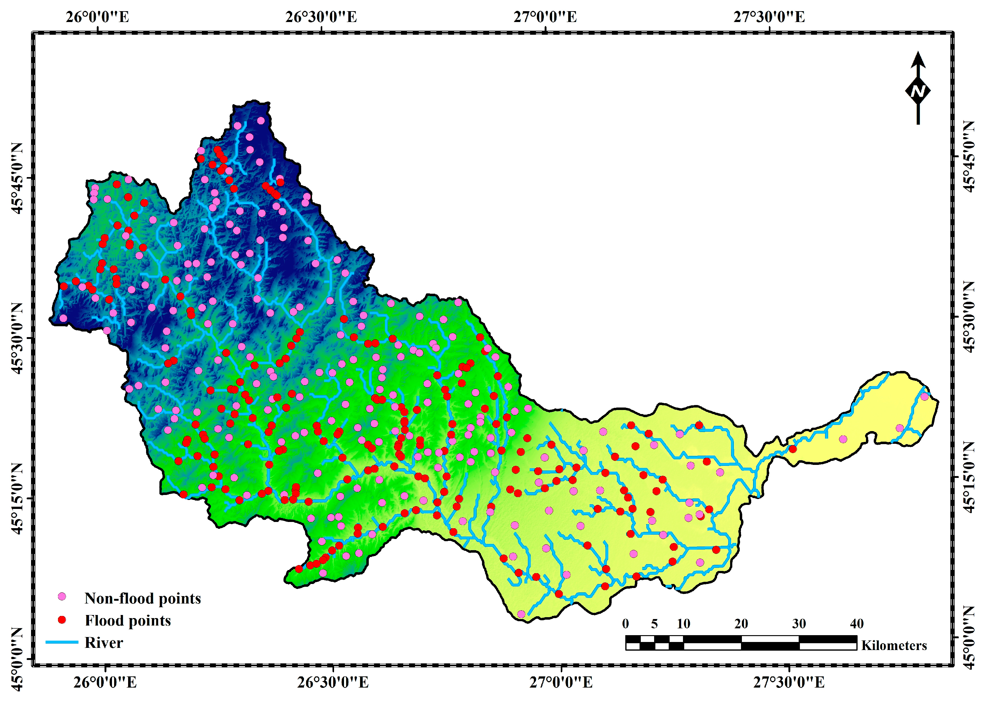
2.1. Study Area: Overview of the Buzău River Catchment

The Buzău River basin (Figure 1) is situated in the south-eastern region of Romania and serves as a left tributary to the Siret River [66]. Originating from the Ciucaș Mountains within the Curvature Carpathians, the Buzău River has an overall length of 302 km [66]. This catchment area encompasses 5264 km² [66] and receives an average annual precipitation of about 750 mm/year [67].

The catchment region covers five counties: Covasna, Brăila, Brașov, Buzău, and Prahova, along with 116 territorial-administrative units [66]. The catchment showcases a varied topography, from the steep northern Carpathian Mountain slopes to the southern low-lying plains. The basin features thick forests in the upper basin, along with agricultural and urbanized zones downstream, where uncontrolled development and land degradation have amplified the risk of flooding. The Buzău River is among the rivers in Romania that face the greatest risk of flooding, having experienced significant flood events in recent decades [66], making it a crucial region for FSM.

2.2. Methodological Framework for Susceptibility Modeling

The modeling process employed a multi-tier feature selection strategy, followed by the application of four ensemble boosting algorithms and multiple evaluation metrics, as well as explainable artificial intelligence (XAI) techniques such as SHAP to analyze flood susceptibility (Figure 2).

The modeling was performed on the Kaggle and Google Colab platforms, which provide cloud-based environments with significant computational power. In this analysis, the pixel served as the main spatial and mapping unit, featuring a spatial resolution of 30 m, which guarantees uniform input across all geospatial layers.

2.3. Flood Inventory Dataset and Data Splitting Strategy

This research compiled a total of 205 locations of flood occurrences from earlier studies conducted by Costache et al. [67,68]. The inventory comprises flood events that resulted in socio-economic damage between 1990 and 2020 [67], categorized as the positive class (indicating flood presence) within the FSM framework. An equivalent number of non-flood points (205) were randomly generated to maintain a balanced dataset from regions with no documented flood history. These non-flood sites represent the negative class (indicating flood absence) and were selected carefully to avoid overlap with flood-affected regions, thus maintaining a clear distinction. The dataset, comprising 410 spatial points (205 flood and 205 non-flood locations), was randomly partitioned into two subsets: 70% of the data (287 points) was designated for model training, and the remaining 30% (123 points) was allocated for model validation (Figure 3). The 70:30 split ratio is commonly employed because it facilitates effective model training and precise performance assessment [69,70].

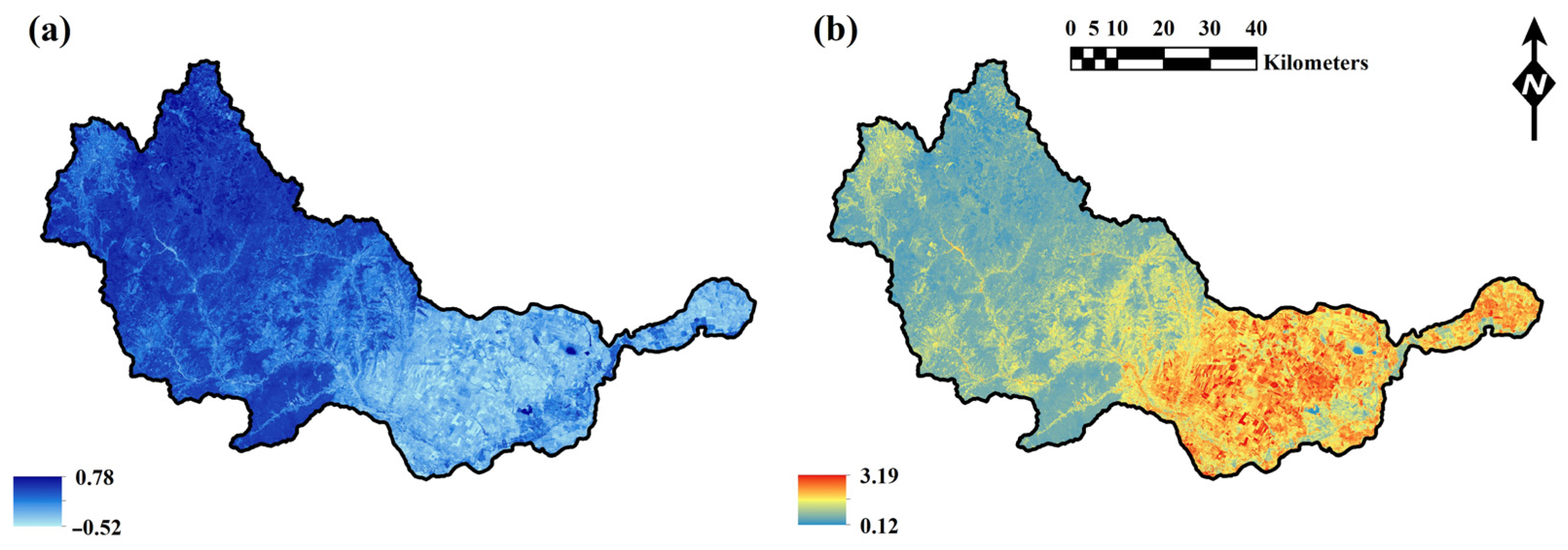
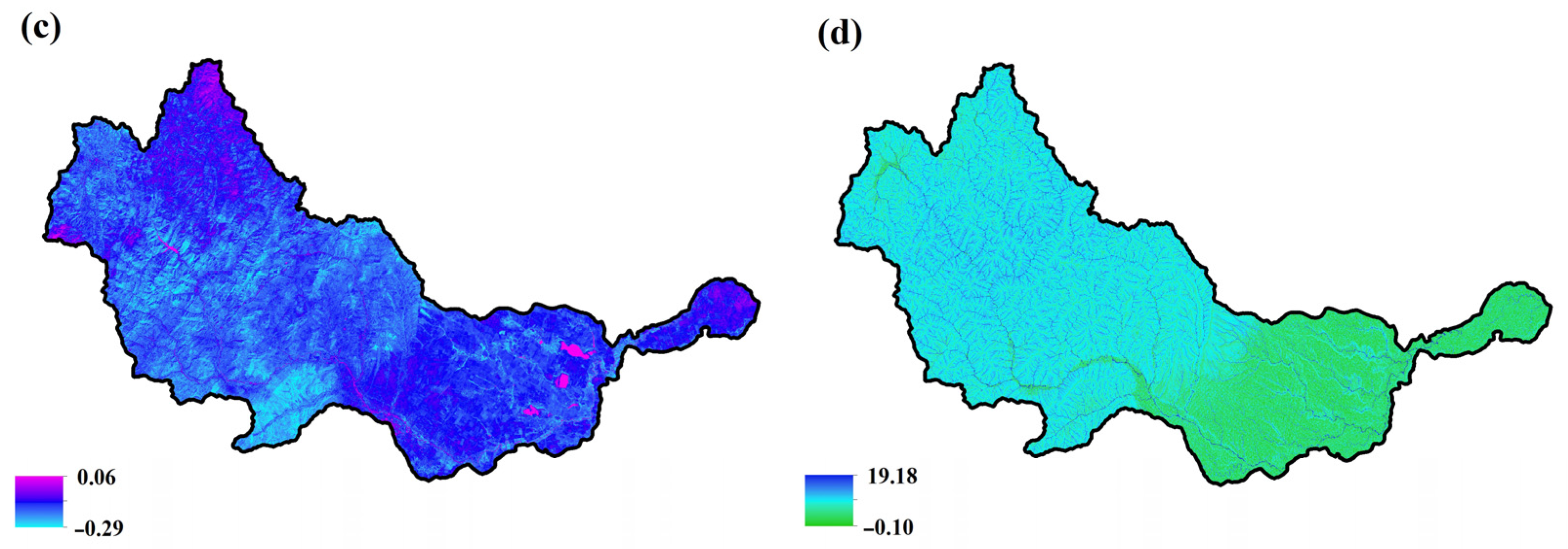
2.4. Derivation of Conditioning Factors

Based on earlier studies [41,71,72,73], the modeling process selected 13 CFs, which are presented in

Table 1. Overview of the datasets and conditioning factors derived for the modeling, including their sources and spatial resolutions.

Dataset	Source	Conditioning Factor	Scale/Spatial Resolution
SRTM DEM	https://earthexplorer.usgs.gov/ (accessed on 20 April 2025)	Slope	30 m
		Elevation
		Stream Power Index (SPI)
		Topographic Wetness Index (TWI)
CORINE Land Cover	https://land.copernicus.eu/en/products/corine-land-cover (accessed on 20 April 2025)	Land Use/Land Cover (LULC)	100 m
SoilGrids	https://soilgrids.org/ (accessed on 20 April 2025)	Soil Clay Content	250 m
		Soil Bulk Density
HydroSHEDS	https://www.hydrosheds.org/products/hydrorivers (accessed on 20 April 2025)	Distance from Rivers	-
Landsat 8 and 9 imagery	https://earthexplorer.usgs.gov/ (accessed on 20 April 2025)	Normalized Difference Impervious Surface Index (NDISI)	100 m
Sentinel-2 imagery	https://browser.dataspace.copernicus.eu/ (accessed on 20 April 2025)	Urban Index (UI)	20 m
		Normalized Difference Greenness Index (NDGI)	10 m
		Normalized Difference Water Index (NDWI)	10 m
		Land Surface Water Index (LSWI)	20 m

.

Slope, elevation, SPI, and TWI were obtained from the DEM utilizing SAGA GIS version 9.5.1 (Institute of Geography at the University of Hamburg). SPI and TWI values were determined based on Equations (1) and (2) [72]. The LULC data were sourced from the CORINE Land Cover portal, whereas the soil clay content and bulk density were acquired from the SoilGrids portal. River networks were obtained from the HydroSHEDS portal (https://www.hydrosheds.org/products), and the distance to these rivers was computed utilizing the Euclidean Distance tool in ArcGIS 10.8 (ESRI, Romania). The five-year (2020–2024) mean UI, NDGI, NDWI, and LSWI were computed using Sentinel-2 surface reflectance data, while NDISI was derived from Landsat 8 and 9 (NASA) data. All five indices were derived using the Google Earth Engine platform, which provides efficient access to multi-temporal satellite imagery and facilitates large-scale geospatial analysis. The selection of a five-year mean aims to mitigate the effects of seasonal and interannual fluctuations, thus providing a more consistent and accurate estimate of land surface conditions. The UI, NDISI, NDGI, NDWI, and LSWI were calculated utilizing Equations (3)–(7) [74,75,76,77,78], respectively.

$$\mathrm{S}\mathrm{P}\mathrm{I}=\alpha \times tan\beta$$

(1)

$$\mathrm{T}\mathrm{W}\mathrm{I}=\mathit{ln}\left({\displaystyle \frac{\alpha }{tan\beta }}\right)$$

(2)

where $\alpha$ = catchment area and $\beta$ = slope angle.

$$\mathrm{U}\mathrm{I}={\displaystyle \frac{SWIR2 -NIR}{SWIR2+NIR}}$$

(3)

$$\mathrm{N}\mathrm{D}\mathrm{I}\mathrm{S}\mathrm{I}={\displaystyle \frac{T_b-(MNDWI+NIR+SWIR1)/3}{T_b+(MNDWI+NIR+SWIR1)/3}}$$

(4)

$$\mathrm{N}\mathrm{D}\mathrm{G}\mathrm{I}={\displaystyle \frac{\alpha \times Green+\left(1-\alpha \right)\times NIR-Red}{\alpha \times Green+\left(1-\alpha \right)\times NIR+Red}}$$

(5)

$$\mathrm{N}\mathrm{D}\mathrm{W}\mathrm{I}={\displaystyle \frac{Green-NIR}{Green+NIR}}$$

(6)

$$\mathrm{L}\mathrm{S}\mathrm{W}\mathrm{I}={\displaystyle \frac{NIR-SWIR}{NIR+SWIR}}$$

(7)

where $T_b$ = brightness temperature, $\alpha$ = weighted parameter, SWIR = Short-Wave Infrared band, NIR = Near-Infrared band, Green = Green band, Red = Red band, and MNDWI = Modified Normalized Difference Water Index [41].

2.5. Feature Selection Techniques

In this modeling, the feature selection process includes the evaluation of multicollinearity and the implementation of feature selection algorithms to discard multicollinear and non-relevant factors. The key challenge posed by multicollinearity is its tendency to inflate standard errors, resulting in unstable estimates and unreliable interpretations [79]. Irrelevant and redundant factors may negatively influence algorithms’ complexity and functionality, leading to suboptimal results or performance [80]. The feature selection process involves removing irrelevant and redundant factors to boost the performance of algorithms and the accuracy of model outputs [80,81].

2.5.1. Variance Inflation Factor (VIF)

VIF is a statistical indicator utilized to measure the degree of multicollinearity among CFs [70]. A VIF score greater than 10 signifies multicollinearity, which was determined through Equation (8) [82]. Typically, researchers discard all factors that have VIF scores exceeding 10 in one step. However, this study implemented a step-wise analysis of multicollinearity and factor removal, which allowed for a more accurate identification and retention of impactful factors. This approach guarantees that only the most problematic factors are omitted, without compromising important predictive data.

$$\mathrm{V}\mathrm{I}\mathrm{F}={\displaystyle \frac{1}{1-R_j^2}}$$

(8)

where $R_j^2$ = coefficient of determination (R²) for the jth factor.

2.5.2. Condition Index (CI)

CI is the square root of the ratio of the maximum eigenvalue to each eigenvalue, as outlined in Equation (9) [83]. Multicollinearity is deemed absent if the CI is 10 or lower, moderate if it ranges from 10 to 30, and severe if it is 30 or higher [84].

$$\mathrm{C}\mathrm{I}=\sqrt{{\displaystyle \frac{{\lambda }_{max}}{{\lambda }_i}}}$$

(9)

where ${\lambda }_{max}$ = maximum eigenvalue and ${\lambda }_i$ = ith eigenvalue.

2.5.3. Mutual Information (MI)

MI is a filter-based approach that measures the degree of interdependence among variables, effectively capturing linear and nonlinear associations [85]. MI is a benchmark for choosing appropriate feature subsets by assessing the quantity of information, feature offers concerning the target variable [86]. MI(X;Y) was computed by applying Equation (10) [85,87].

$$\mathrm{M}\mathrm{I}(X;Y)=\sum _{x\in X}\sum _{y\in Y}p\left(x,y\right) log\left({\displaystyle \frac{p(x,y)}{p\left(x\right) p\left(y\right)}}\right)$$

(10)

where X and Y = two random variables, $p\left(x,y\right)$ = joint probability distribution, and $p\left(x\right)$ and $p\left(y\right)$ = marginal distributions.

2.5.4. Information Gain (IG)

IG is an entropy-based approach that evaluates the information supplied by a feature [81]. The gain (y, A), calculated from the output data categorized by feature A, was computed according to Equation (11) [88].

$$\mathrm{g}\mathrm{a}\mathrm{i}\mathrm{n}\left(y,A\right)=entropy\left(y\right)-{\sum }_{C\in vals\left(A\right)}{\displaystyle \frac{y_c}{y}}entropy \left(y_c\right)$$

(11)

with val(A) = possible values of feature A, $y$ = number of samples, and $y_c$ = subset of $y$.

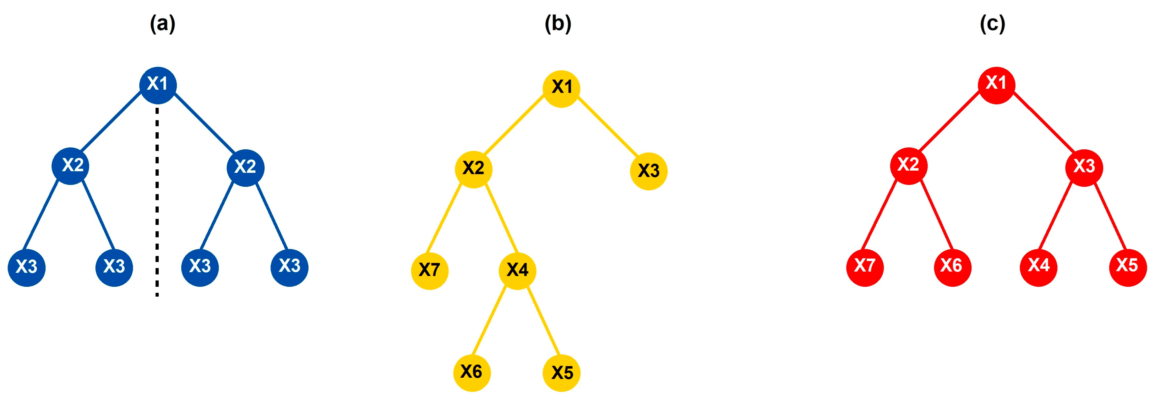
2.6. Machine Learning (ML) Algorithms

2.6.1. Adaptive Boosting (AdaBoost)

AdaBoost is an algorithm based on decision trees that creates a collection of stumps, which are basic trees consisting of a single node and two leaves, typically only one level deep [89,90]. It adopts an iterative approach to learn from these stumps and integrates them into an ensemble [90]. AdaBoost operates by minimizing an exponential loss function, making it sensitive to data noise and outliers [91]. Despite this challenge, it effectively decreases bias and variance, improving overall performance [91].

2.6.2. Gradient Boosting Algorithms

Categorical Boosting (CatBoost): CatBoost can efficiently address both categorical and numerical factors without requiring preprocessing steps such as one-hot encoding or label encoding, instead relying on its inherent ‘ordered boosting’ approach to manage categorical data [92]. Each model is trained on fresh data by utilizing ordered boosting, which helps alleviate the biases commonly linked to standard GB algorithms [91]. CatBoost employs ‘oblivious decision trees’ (Figure 4a), which maintain the same splitting criterion at every tree level, creating balanced structures that are less likely to overfit [93,94].

Light Gradient Boosting Machine (LightGBM): LightGBM presents three novel strategies designed to enhance the efficiency of training: a histogram-based approach for split finding, Exclusive Feature Bundling (EFB), and Gradient-Based One-Side Sampling (GOSS) [92,93]. The histogram-based split finding technique accelerates the training and reduces memory requirements by binning continuous feature values before identifying the best splits [92]. EFB applies heuristics to identify and merge groups of mutually exclusive features, decreasing the dataset’s dimensionality [93]. GOSS utilizes gradients to sample the most critical instances of the dataset during each iteration, ensuring the training set distribution remains unchanged [93]. LightGBM builds trees leaf-wise (Figure 4b), resulting in quicker convergence and greater accuracy [91].

eXtreme Gradient Boosting (XGBoost): XGBoost builds additive models sequentially, allowing for the optimization of any differentiable loss function [91]. It incorporates regularization techniques (L1 and L2) to reduce overfitting, thereby enhancing the model’s ability to generalize [91]. Additionally, XGBoost applies second-order Taylor series approximations of the loss function to improve both accuracy and computational efficiency [59,91]. It supports parallel processing and internally addresses missing values [91]. XGBoost mainly follows a level-wise tree growth strategy (Figure 4c), where all nodes at a specific depth are split before advancing deeper, which helps control overfitting and maintain balanced trees [94].

2.7. Performance Evaluation Techniques

2.7.1. Mean Absolute Error (MAE) and Root Mean Square Error (RMSE)

MAE and RMSE serve as key indicators of absolute error, primarily applied in model fitting, validation, selection, and comparison [95]. The MAE and RMSE values were computed based on Equations (12) and (13) [51].

$$\mathrm{M}\mathrm{A}\mathrm{E}={\displaystyle \frac{1}{n}}\sum _{i=1}^n\left|Y_i-{\tilde{Y}}_i\right|$$

(12)

$$\mathrm{R}\mathrm{M}\mathrm{S}\mathrm{E}=\sqrt{{\displaystyle \frac{1}{n}}\sum _{i=1}^n{(Y_i-{\tilde{Y}}_i)}^2}$$

(13)

where $Y_i$ = actual value, ${\tilde{Y}}_i$ = predicted value, and n = number of observations.

2.7.2. R-Squared (R²)

The R-squared (R²) serves as a quantitative measure of how effectively a model captures the variability of the dependent factor as influenced by the independent factors [96]. It represents the proportion of the variation explained by the model out of the overall variation [51], with possible values spanning from 0 (indicating a lack of fit) to 1 (indicating a perfect fit) [97]. R² was derived through the application of Equation (14) [51].

$${\mathrm{R}}^2=1-{\displaystyle \frac{\sum _1^n{\left(D_{act}-D_{pre}\right)}^2}{\sum _1^n{\left(D_{act}-{\overline{D}}_{act}\right)}^2}}$$

(14)

where $D_{act}$ = actual value, $D_{pre}$ = predicted value, ${\overline{D}}_{act}$ = mean, and n = number of observations.

2.7.3. Accuracy, Precision, Recall, and F1-Score

Accuracy, precision, recall, and F1-score, key performance metrics ranging from 0 (denoting poor performance) to 1 (denoting perfect performance), were computed using Equations (15)–(18) [82,98], respectively.

$$\mathrm{A}\mathrm{c}\mathrm{c}\mathrm{u}\mathrm{r}\mathrm{a}\mathrm{c}\mathrm{y}={\displaystyle \frac{TP+TN}{TP+FP+FN+TN}}$$

(15)

$$\mathrm{P}\mathrm{r}\mathrm{e}\mathrm{c}\mathrm{i}\mathrm{s}\mathrm{i}\mathrm{o}\mathrm{n}={\displaystyle \frac{TP}{TP+FP}}$$

(16)

$$\mathrm{R}\mathrm{e}\mathrm{c}\mathrm{a}\mathrm{l}\mathrm{l}={\displaystyle \frac{TP}{TP+FN}}$$

(17)

$$\mathrm{F}1\text{-}\mathrm{s}\mathrm{c}\mathrm{o}\mathrm{r}\mathrm{e}=2\times {\displaystyle \frac{Precision\times Recall}{Precision+Recall}}$$

(18)

where TP (TN) = True Positives (Negatives), FP (FN) = False Positives (Negatives).

2.7.4. Kappa Index (κ-Index)

Cohen’s Kappa index (κ-index) is a statistical indicator that evaluates the extent of agreement, with values spanning −1 to +1 [82,99]. A score of −1 reflects total disagreement, 0 indicates a lack of agreement beyond random chance, and +1 signifies total agreement [82,99]. The κ-index was derived based on Equation (19) [82].

$$\mathsf{\kappa }\text{-}\mathrm{i}\mathrm{n}\mathrm{d}\mathrm{e}\mathrm{x}={\displaystyle \frac{P_{obs}-P_{exp}}{1-P_{exp}}}$$

(19)

where $P_{obs}$ = observed agreement and $P_{exp}$ = expected agreement.

2.7.5. Receiver Operating Characteristic (ROC) Curve

The ROC curve represents a graph that plots the True Positive Rate (TPR) on the Y-axis against the False Positive Rate (FPR) on the X-axis, serving as a measure of overall performance [100,101]. The area under the ROC Curve (AUC) is applied to quantify this performance [100], with AUC values ranging from 0.5 (random performance) to 1 (perfect performance) [102].

2.7.6. Precision Recall Curve (PRC)

The PRC, featuring recall on the X-axis and precision on the Y-axis, is regarded as a more informative tool than the ROC curve for evaluating performance in datasets with class imbalance [103]. Higher average precision (AP) scores signify superior model performance, with a score of 1 indicating perfect performance and 0 denoting poor performance [104].

2.8. Factor Importance Evaluation: SHapley Additive exPlanations (SHAP)

SHAP elucidates a prediction by illustrating the contribution of each feature to the variation from the model’s baseline value [105,106]. It is grounded in coalitional game theory [105] and employs a linear explanatory model (Equation (20)) to approximate the original prediction model [107,108]. SHAP will quantify and visualize the impact of each conditioning factor on the predictions made by the model. This will facilitate a more profound comprehension of the relative significance of each factor in relation to flood susceptibility, thus improving the interpretability of the model and aiding in more informed decision-making.

$$f\left(x\right)=g\left(x^{\prime }\right)={\varnothing }_0+\sum _{i=1}^M{\varnothing }_i{x}_i^{\prime }$$

(20)

where $f\left(x\right)$ = original model, $g\left(x^{\prime }\right)$ = explanation model, M = number of input features, ${\varnothing }_0$ = base value, ${\varnothing }_i$ = SHAP value, and $x_i^{\prime }\in \left\{\mathrm{0,1}\right\}$ = presence (1) or absence (0) of the i-th feature.

The computation of the SHAP value was performed based on Equation (21) [107].

$${\varnothing }_i=\sum _{z^{\prime }\subseteq x^{\prime }\backslash \left\{i\right\}}{\displaystyle \frac{\left|z^{\prime }\right|!·(M -\left|z^{\prime }\right| -1)!}{M!}}\left[f_x\left(z^{\prime }\cup \left\{i\right\}\right) -f_x\left(z^{\prime }\right)\right]$$

(21)

where $z^{\prime }\subseteq x^{\prime }\backslash \left\{i\right\}$ = potential subsets of the simplified input, without feature $i$, $\left|z^{\prime }\right|$ = number of features in the subset $z^{\prime }$, ${\displaystyle \frac{\left|z^{\prime }\right|!·(M -\left|z^{\prime }\right| -1)!}{M!}}$ = SHAP weight, $f_x(z^{\prime }\cup \left\{i\right\})$ = output of the model when utilizing subset $z^{\prime }$ with feature $i$, and $f_x\left(z^{\prime }\right)$ = model output when utilizing solely the subset $z^{\prime }$.

3. Results

3.1. Conditioning Factors Selected Through Various Feature Selection Methods

An analysis of the multicollinearity for the 13 CFs was performed, identifying three factors with VIF scores surpassing 10 (

Table A1. Initial VIF scores of all conditioning factors before removal of multicollinear factors.

Sl. No.	Conditioning Factor	VIF Score
1	LSWI	138.576
2	UI	68.691
3	NDISI	33.641
4	Soil Clay Content	8.081
5	NDGI	7.756
6	Soil Bulk Density	6.694
7	TWI	4.996
8	Elevation	3.594
9	Slope	3.592
10	SPI	3.234
11	NDWI	2.570
12	Distance from Rivers	1.487
13	LULC	1.378

). To mitigate this issue, a two-tier selection approach was implemented. During the first stage, the factor with the highest VIF score, LSWI, was discarded, and the multicollinearity was re-evaluated, indicating that two CFs continued to display multicollinearity (

Table A2. VIF scores after the first iteration of removing the most collinear conditioning factor.

Sl. No.	Conditioning Factor	VIF Score
1	UI	23.294
2	NDISI	20.292
3	Soil Clay Content	7.857
4	NDGI	6.603
5	Soil Bulk Density	6.569
6	TWI	4.949
7	Slope	3.583
8	SPI	3.170
9	Elevation	3.048
10	NDWI	2.309
11	Distance from Rivers	1.487
12	LULC	1.373

). At the second stage, the subsequent factor with the highest VIF score (UI) was removed, and the multicollinearity was re-evaluated (

Table 2. Variance Inflation Factor (VIF) scores of the conditioning factors.

Sl. No.	Conditioning Factor	VIF Score
1	Soil Clay Content	7.844
2	Soil Bulk Density	6.548
3	NDGI	6.330
4	NDISI	5.566
5	TWI	4.888
6	Slope	3.539
7	SPI	3.072
8	Elevation	2.872
9	NDWI	1.763
10	Distance from Rivers	1.486
11	LULC	1.360

).

Thus, it was established that all remaining 11 CFs maintained VIF scores beneath the threshold of 10. In addition, the CI for all 11 CFs was determined to be beneath the critical threshold of 30 (

Table 3. Condition index (CI) of the conditioning factors used in the modeling.

Sl. No.	Conditioning Factor	CI
1	TWI	7.550
2	Distance from Rivers	6.490
3	SPI	5.810
4	Slope	3.400
5	NDWI	2.960
6	NDISI	2.460
7	NDGI	2.360
8	LULC	1.940
9	Elevation	1.570
10	Soil Bulk Density	1.310
11	Soil Clay Content	1.000

), thereby validating that all multicollinear factors have been effectively eliminated.

To ensure the exclusion of irrelevant factors, the MI scores for the 11 CFs were computed. The analysis revealed that Slope (0.452), TWI (0.403), and Distance from Rivers (0.348) had the highest MI scores, indicating their significant relevance for inclusion, while Soil Clay Content (0.042) and NDWI (0.012) displayed the lowest MI scores, implying minimal relevance (

Table 4. Conditioning factors and their corresponding Mutual Information (MI) scores.

Sl. No.	Conditioning Factor	MI Score
1	Slope	0.452
2	TWI	0.403
3	Distance from Rivers	0.348
4	SPI	0.211
5	LULC	0.187
6	Elevation	0.146
7	Soil Bulk Density	0.141
8	NDGI	0.107
9	NDISI	0.100
10	Soil Clay Content	0.042
11	NDWI	0.012

). Despite the variation in scores, none were zero, and therefore all 11 CFs were retained for subsequent analysis.

Subsequently, IG-based feature selection was implemented due to its effectiveness with tree-based ML algorithms. The analysis demonstrated that SPI (0.000) and NDWI (0.001) exhibited negligible IG scores (

Table 5. Information Gain (IG) scores of the conditioning factors.

Sl. No.	Conditioning Factor	IG Score
1	Slope	0.451
2	Distance from Rivers	0.400
3	TWI	0.375
4	LULC	0.326
5	NDGI	0.116
6	NDISI	0.110
7	Elevation	0.099
8	Soil Bulk Density	0.088
9	Soil Clay Content	0.007
10	NDWI	0.001
11	SPI	0.000

), reflecting their limited relevance; thus, these two factors were discarded. Consequently, the multi-tier feature selection approach led to the identification of nine relevant factors (Figure 5 and Figure 6) and the elimination of four irrelevant factors (Figure A1).

3.2. Flood Susceptibility Models and Their Performance

The susceptibility maps were produced utilizing four ML models—AdaBoost (Figure 7a), CatBoost (Figure 7b), LightGBM (Figure 7c), and XGBoost (Figure 7d)—based on nine CFs. All maps pinpointed the river network and low-lying regions as areas of significant susceptibility.

Table 6. Performance evaluation of the models using MAE, RMSE, and R² metrics on both training and testing datasets.

Model	MAE		RMSE		R2
	Train	Test	Train	Test	Train	Test
AdaBoost	0.088	0.117	0.173	0.229	0.880	0.787
CatBoost	0.074	0.097	0.146	0.182	0.919	0.838
LightGBM	0.082	0.111	0.164	0.211	0.892	0.804
XGBoost	0.079	0.102	0.151	0.192	0.914	0.817

illustrates the models’ performance as measured by MAE, RMSE, and R² for both datasets. CatBoost exhibited the most superior performance, recording the lowest MAE (0.074) and RMSE (0.146) on the training set, as well as the lowest MAE (0.097) and RMSE (0.182) on the testing set. It also achieved the highest R² scores of 0.919 and 0.838 for the training and testing sets, respectively.

3.3. Results of Susceptibility Model Evaluation Using Various Performance Metrics

Among the assessed models, CatBoost excelled with a precision of 0.928, recall of 0.917, F1-score of 0.913, accuracy of 0.912, and a κ-index of 0.841, as indicated in

Table 7. Performance comparison of flood susceptibility models using various evaluation metrics.

	AdaBoost	CatBoost	LightGBM	XGBoost
Precision	0.904	0.928	0.906	0.916
Recall	0.887	0.917	0.885	0.909
F1-Score	0.885	0.913	0.894	0.908
Accuracy	0.886	0.912	0.894	0.908
κ-index	0.782	0.841	0.801	0.825

. It consistently achieved superior results compared to AdaBoost, LightGBM, and XGBoost.

In addition, CatBoost achieved the best overall performance, reaching the highest ROC-AUC score of 0.972, trailed by XGBoost with 0.971, LightGBM with 0.967, and AdaBoost with 0.964 (Figure 8).

The PRC-AP was similarly the highest for CatBoost (0.971), followed by XGBoost (0.967), AdaBoost (0.963), and LightGBM (0.961) (Figure 9). These findings underscore the enhanced capability of GB models—CatBoost, XGBoost, and LightGBM—compared to AdaBoost.

4. Discussion

4.1. Role and Importance of Conditioning Factors

The SHAP-driven factor importance assessment for the CatBoost model, identified as the top performer, revealed that Slope (0.232) and Distance from Rivers (0.155) were the most influential CFs (

Table 8. SHAP-based importance of conditioning factors (mean absolute SHAP).

Sl. No.	Conditioning Factor	Mean_Abs_SHAP
1	Slope	0.232
2	Distance from Rivers	0.155
3	TWI	0.061
4	LULC	0.034
5	NDISI	0.026
6	Soil Bulk Density	0.022
7	Elevation	0.019
8	NDGI	0.017
9	Soil Clay Content	0.015

). The SHAP summary plot (Figure 10) visually represents how each factor influences the model’s predictions, emphasizing that Slope and Distance from Rivers contributed most significantly and consistently across the dataset. Many studies [61,71,109] have identified Slope, Distance from Rivers, and LULC as key contributing factors. Specifically, Costache et al. [68] reported these three as the most influential CFs in the Buzău River catchment.

Slope, with a mean SHAP value of 0.232, stands out as the most critical factor, likely due to its strong effect on surface runoff and water accumulation processes. Steeper slopes facilitate greater surface runoff and limit infiltration, while flatter terrains tend to gather water, thus amplifying flood risks [110,111]. Ranking second (0.155), the Distance from Rivers illustrates the vulnerability of areas adjacent to river channels. Areas near rivers face higher risk due to the immediate impact of river overflow during periods of high discharge; during heavy rainfall, rising river levels tend to inundate the surrounding low-lying regions first [112,113]. TWI (0.061) exhibited a notable impact, emphasizing the crucial role of terrain morphology in retaining water and directing flow. The TWI indicates possible water accumulation within the landscape; elevated values signify areas at risk of saturation and runoff concentration, which can lead to flooding [72,114].

LULC has a moderate contribution of 0.034, suggesting that land management practices and surface conditions play a significant role in flooding. LULC impacts flooding by altering land–rainfall interactions, where urban and agricultural regions enhance surface runoff due to their reduced capacity for infiltration [41,115]. The compaction of soil on agricultural land, caused by heavy machinery and livestock, can facilitate flooding by reducing permeability and hindering water infiltration [116,117]. Moreover, repeated tilling can result in the loss of organic matter and degradation of soil structure [118], consequently heightening surface runoff during heavy rainfall events. Furthermore, the transformation of natural vegetation into agricultural land removes deep-rooted plants that play a crucial role in absorbing and regulating rainwater. Irrigation methods and inadequate drainage can lead to soil saturation, which reduces its ability to absorb further rainfall and raises the risk of flooding [119].

Among the moderately important factors, NDISI (0.026) and Soil Bulk Density (0.022) exhibited limited but relevant influences, indicating secondary contributions to flood occurrence. Higher NDISI values reflect impervious surfaces such as roads and buildings [120], which hinder infiltration and amplify surface runoff, consequently raising the chance of flooding [121,122]. Prior investigations [4,123] emphasized the impact of soil sealing on flooding, illustrating how alterations to the natural hydraulic network can lead to increased flood risk. An increase in bulk density results in reduced soil porosity and infiltration [124], which consequently heightens the probability of surface runoff and flooding.

Elevation plays a crucial role by dictating the natural pathways for water flow; regions at lower elevations are more likely to gather runoff and are at a higher risk of inundation, especially in the event of significant rainfall or river surges [111,125]. NDGI assesses the density and health of vegetation, reflecting trends of degradation and regeneration [126]. Areas with lower NDGI, which denote sparse or unhealthy vegetation [126,127], can heighten the probability of flooding due to the diminished ability of the soil to absorb water, thereby facilitating quicker surface runoff [128]. Clay-dominant soils possess lower permeability, which hinders infiltration and allows for water to remain for longer durations, consequently promoting flooding [41,129].

The SHAP analysis indicates that elevation (0.019), NDGI (0.017), and Soil Clay Content (0.015) have a relatively minor significance, implying their limited effect in the Buzău catchment. Although elevation typically influences hydrological flow and retention behavior, the Buzău catchment may feature localized flooding events that are more concentrated in topographically low areas, irrespective of their absolute elevation. Consequently, local variations in elevation—such as depressions or valleys—may be more significant than the overall elevation.

The NDGI, indicative of vegetation greenness, may have a limited impact during intense rainfall events, as vegetation’s ability to reduce runoff diminishes. Likewise, while the clay content in soil can play a role in determining infiltration capacity, this effect may be overshadowed by other soil characteristics, including bulk density. This analysis indicates that although these factors are not entirely irrelevant, their influence is relatively limited within this modeling framework.

4.2. Interpretation of Model Performance Outcomes

The modeling process revealed that CatBoost achieved the highest performance, with XGBoost, LightGBM, and AdaBoost ranking next. Several studies [58,59,89,91,94,130,131,132] have identified CatBoost as the most effective model among GB algorithms. In contrast, other research has found that XGBoost [93] or LightGBM [60,133] may be more effective. This variation in results underscores the significance of dataset characteristics, feature composition, and preprocessing techniques in determining model efficacy. The superior performance of CatBoost can be linked to its ability to effectively handle categorical variables without one-hot encoding, as well as its application of ordered boosting and symmetric (oblivious) trees [51,134]. These characteristics are recognized for boosting model accuracy and decreasing overfitting [51,134]. This is particularly useful in FSM, where both continuous and categorical inputs are commonly utilized.

XGBoost also demonstrated commendable performance, probably owing to its well-optimized training architecture, proficient parallel processing capabilities, and flexibility regarding objective functions [135,136]. Moreover, its advanced regularization techniques contribute to enhanced generalizability [135]. LightGBM employs a leaf-wise tree growth strategy that is efficient, yet it can cause instability in datasets that are smaller or contain noise [137]. This could account for its comparatively lower performance in this modeling, indicating that LightGBM may be less appropriate for FSM tasks that involve spatial heterogeneity or class imbalance. In this comparison, AdaBoost demonstrated the lowest performance. This is due to its vulnerability to noisy data and outliers, as it amplifies the weight of misclassified instances, which may diminish the overall performance when compared to GB algorithms [138]. Overall, the results bolster the prevailing view that CatBoost is a robust and effective option, especially when dealing with categorical factors. These conclusions are in line with recent literature and stress the need for model selection to be adapted to the specific characteristics of the dataset and the goals of the modeling process.

5. Conclusions

This research emphasizes the efficacy of ensemble boosting algorithms, especially CatBoost, for FSM in the Buzău River catchment, an ecologically and hydrologically sensitive region within the Danube River Basin. Through the integration of multi-tier feature selection and SHAP-based interpretability, this research not only boosts model accuracy but also improves transparency in recognizing essential factors driving floods. The study reveals that Slope, Distance from Rivers, TWI, and LULC are key contributors to flood susceptibility in this catchment. From a policy viewpoint, the conclusions endorse the necessity for targeted land-use planning measures, including more rigorous zoning regulations in critical areas and the integration of sustainable practices in watershed management. Authorities must prioritize the protection and surveillance of low-lying zones and riverine areas while also incorporating topographic and hydrological information into regional disaster management plans. The methodological framework outlined in this research can be adapted to other flood-prone locales and underscores the critical need for science-driven policies to foster climate-resilient communities.

One notable limitation of this study is the lack of an in-depth analysis of model uncertainty and sensitivity testing. Although performance metrics were employed to assess the model, they do not completely encompass the range of uncertainty present in the input data, model parameters, or algorithmic framework, nor do they evaluate the model’s sensitivity to variations in individual input factors. Moreover, the analysis incorporated CORINE Land Cover data from 2018, which is the most current dataset that is available. Despite the application of more recent RS-based indices to reflect current surface conditions, the reliance on 2018 land cover data may restrict the accurate representation of the most recent LULC conditions.

References

1. Petrucci, O.; Aceto, L.; Bianchi, C.; Bigot, V.; Brázdil, R.; Pereira, S.; Kahraman, A.; Kılıç, Ö.; Kotroni, V.; Llasat, M.C.; et al. Flood Fatalities in Europe, 1980–2018: Variability, Features, and Lessons to Learn. Water 2019, 11, 1682. [Google Scholar] [CrossRef]
2. Chen, J.; Shi, X.; Gu, L.; Wu, G.; Su, T.; Wang, H.M.; Kim, J.S.; Zhang, L.; Xiong, L. Impacts of Climate Warming on Global Floods and Their Implication to Current Flood Defense Standards. J. Hydrol. 2023, 618, 129236. [Google Scholar] [CrossRef]
3. Furtak, K.; Wolińska, A. The Impact of Extreme Weather Events as a Consequence of Climate Change on the Soil Moisture and on the Quality of the Soil Environment and Agriculture—A Review. CATENA 2023, 231, 107378. [Google Scholar] [CrossRef]
4. Gatto, A.; Martellozzo, F.; Clo’, S.; Ciulla, L.; Segoni, S. The Downward Spiral Entangling Soil Sealing and Hydrogeological Disasters. Environ. Res. Lett. 2024, 19, 084023. [Google Scholar] [CrossRef]
5. Liu, Q.; Du, M.; Wang, Y.; Deng, J.; Yan, W.; Qin, C.; Liu, M.; Liu, J. Global, Regional and National Trends and Impacts of Natural Floods, 1990–2022. Bull. World Health Organ. 2024, 102, 410–420. [Google Scholar] [CrossRef]
6. Paprotny, D.; Terefenko, P.; Śledziowski, J. HANZE v2.1: An Improved Database of Flood Impacts in Europe from 1870 to 2020. Earth Syst. Sci. Data 2024, 16, 5145–5170. [Google Scholar] [CrossRef]
7. Economic Losses from Weather- and Climate-Related Extremes in Europe. Available online: https://www.eea.europa.eu/en/analysis/indicators/economic-losses-from-climate-related (accessed on 13 May 2025).
8. Morlot, M.; Brilly, M.; Šraj, M. Characterisation of the Floods in the Danube River Basin through Flood Frequency and Seasonality Analysis. Acta Hydrotech. 2019, 32, 73–89. [Google Scholar] [CrossRef]
9. Bezak, N.; Petan, S.; Kobold, M.; Brilly, M.; Bálint, Z.; Balabanova, S.; Cazac, V.; Csík, A.; Godina, R.; Janál, P.; et al. A Catalogue of the Flood Forecasting Practices in the Danube River Basin. River Res. Appl. 2021, 37, 909–918. [Google Scholar] [CrossRef]
10. Leščešen, I.; Basarin, B.; Pavić, D.; Mudelsee, M.; Pekarova, P.; Mesaroš, M. Are Extreme Floods on the Danube River Becoming More Frequent? A Case Study of Bratislava Station. J. Water Clim. Chang. 2024, 15, 1300–1312. [Google Scholar] [CrossRef]
11. Hein, T.; Schwarz, U.; Habersack, H.; Nichersu, I.; Preiner, S.; Willby, N.; Weigelhofer, G. Current Status and Restoration Options for Floodplains along the Danube River. Sci. Total Environ. 2016, 543, 778–790. [Google Scholar] [CrossRef]
12. Eder, M.; Perosa, F.; Hohensinner, S.; Tritthart, M.; Scheuer, S.; Gelhaus, M.; Cyffka, B.; Kiss, T.; Van Leeuwen, B.; Tobak, Z.; et al. How Can We Identify Active, Former, and Potential Floodplains? Methods and Lessons Learned from the Danube River. Water 2022, 14, 2295. [Google Scholar] [CrossRef]
13. Romanescu, G.; Stoleriu, C. Causes and Effects of the Catastrophic Flooding on the Siret River (Romania) in July–August 2008. Nat. Hazards 2013, 69, 1351–1367. [Google Scholar] [CrossRef]
14. Romanescu, G.; Cimpianu, C.I.; Mihu-Pintilie, A.; Stoleriu, C.C. Historic Flood Events in NE Romania (Post-1990). J. Maps 2017, 13, 787–798. [Google Scholar] [CrossRef]
15. Sekulova, F.; van den Bergh, J.C.J.M. Floods and Happiness: Empirical Evidence from Bulgaria. Ecol. Econ. 2016, 126, 51–57. [Google Scholar] [CrossRef]
16. Momčilović Petronijević, A.; Petronijević, P. Floods and Their Impact on Cultural Heritage—A Case Study of Southern and Eastern Serbia. Sustainability 2022, 14, 14680. [Google Scholar] [CrossRef]
17. Petrović, A.M.; Leščešen, I.; Radevski, I. Unveiling Torrential Flood Dynamics: A Comprehensive Study of Spatio-Temporal Patterns in the Šumadija Region, Serbia. Water 2024, 16, 991. [Google Scholar] [CrossRef]
18. Ana, J. Assessment of Pluvial Floods Potential on the Rivers of the Republic of Moldova. Present Environ. Sustain. Dev. 2018, 12, 121–133. [Google Scholar] [CrossRef]
19. Agayar, E.; Armon, M.; Wernli, H. The Catastrophic Floods in 2008, 2010 and 2020 in Western Ukraine: Hydrometeorological Processes and the Role of Upper-Level Dynamics. In Proceedings of the EGU General Assembly 2025, Vienna, Austria, 27 April–2 May 2025. [Google Scholar] [CrossRef]
20. Albano, R.; Samela, C.; Crăciun, I.; Manfreda, S.; Adamowski, J.; Sole, A.; Sivertun, Å.; Ozunu, A. Large Scale Flood Risk Mapping in Data Scarce Environments: An Application for Romania. Water 2020, 12, 1834. [Google Scholar] [CrossRef]
21. Albulescu, A.C. Exploring the Links between Flood Events and the COVID-19 Infection Cases in Romania in the New Multi-Hazard-Prone Era. Nat. Hazards 2023, 117, 1611–1631. [Google Scholar] [CrossRef]
22. Armaş, I.; Dobre, D.; Fekete, A.; Rufat, S.; Albulescu, A.C. Hinging on the Preparedness of First Responders. A Case Study on the 2021 Flood Operations in Romania. Int. J. Disaster Risk Red. 2025, 116, 105008. [Google Scholar] [CrossRef]
23. Costache, R.; Crăciun, A.; Ciobotaru, N.; Bărbulescu, A. Intelligent Methods for Estimating the Flood Susceptibility in the Danube Delta, Romania. Water 2024, 16, 3511. [Google Scholar] [CrossRef]
24. Popescu, N.C.; Bărbulescu, A. A Practical Approach on Reducing the Flood Impact: A Case Study from Romania. Appl. Sci. 2024, 14, 10378. [Google Scholar] [CrossRef]
25. Popa, M.C.; Simion, A.G.; Peptenatu, D.; Dima, C.; Draghici, C.C.; Florescu, M.; Dobrea, C.R.; Diaconu, D.C. Spatial Assessment of Flash-flood Vulnerability in the Moldova River Catchment (N Romania) Using the FFPI. J. Flood Risk Manag. 2020, 13, e12624. [Google Scholar] [CrossRef]
26. Costache, R.; Arabameri, A.; Costache, I.; Crăciun, A.; Md Towfiqul Islam, A.R.; Abba, S.I.; Sahana, M.; Pham, B.T. Flood Susceptibility Evaluation through Deep Learning Optimizer Ensembles and GIS Techniques. J. Environ. Manag. 2022, 316, 115316. [Google Scholar] [CrossRef]
27. Ionescu, C.S.; Gogoașe-Nistoran, D.E.; Baciu, C.A.; Cozma, A.; Motovilnic, I.; Brașovanu, L. The Impact of a Clay-Core Embankment Dam Break on the Flood Wave Characteristics. Hydrology 2025, 12, 56. [Google Scholar] [CrossRef]
28. Constantin-Horia, B.; Simona, S.; Gabriela, P.; Adrian, S. Human Factors in the Floods of Romania. In Proceedings of the Threats to Global Water Security; Jones, J.A.A., Vardanian, T.G., Hakopian, C., Eds.; Springer: Dordrecht, The Netherlands, 2009; pp. 187–192. [Google Scholar] [CrossRef]
29. Peptenatu, D.; Grecu, A.; Simion, A.G.; Gruia, K.A.; Andronache, I.; Draghici, C.C.; Diaconu, D.C. Deforestation and Frequency of Floods in Romania. In Water Resources Management in Romania; Negm, A.M., Romanescu, G., Zeleňáková, M., Eds.; Springer International Publishing: Cham, Switzerland, 2020; pp. 279–306. [Google Scholar] [CrossRef]
30. World Bank. Romania Water Diagnostic Report: Moving Toward EU Compliance, Inclusion, and Water Security; World Bank: Washington, DC, USA, 2018. [Google Scholar]
31. Cojoc, G.M.; Romanescu, G.; Tirnovan, A. Exceptional Floods on a Developed River: Case Study for the Bistrita River from the Eastern Carpathians (Romania). Nat. Hazards 2015, 77, 1421–1451. [Google Scholar] [CrossRef]
32. Stancalie, G.; Craciunescu, V.; Irimescu, A. Development of a Downstream Emergency Response Service for Flood and Related Risks in Romania Based on Satellite Data. E3S Web Conf. 2016, 7, 17007. [Google Scholar] [CrossRef]
33. Tudose, N.C.; Ungurean, C.; Davidescu, Ș.; Clinciu, I.; Marin, M.; Nita, M.D.; Adorjani, A.; Davidescu, A. Torrential Flood Risk Assessment and Environmentally Friendly Solutions for Small Catchments Located in the Romania Natura 2000 Sites Ciucas, Postavaru and Piatra Mare. Sci. Total Environ. 2020, 698, 134271. [Google Scholar] [CrossRef]
34. Romanescu, G.; Stoleriu, C.C. Exceptional Floods in the Prut Basin, Romania, in the Context of Heavy Rains in the Summer of 2010. Nat. Hazard. Earth Syst. Sci. 2017, 17, 381–396. [Google Scholar] [CrossRef]
35. Ionita, M.; Nagavciuc, V. Shedding Light on the Devastating Floods in June 1897 in Romania: Early Instrumental Observations and Synoptic Analysis. J. Hydrometeorol. 2024, 25, 1729–1745. [Google Scholar] [CrossRef]
36. Romania: Floods-DREF Operation N° MDRRO006—Romania|ReliefWeb. Available online: https://reliefweb.int/report/romania/romania-floods-dref-operation-ndeg-mdrro006 (accessed on 26 May 2025).
37. Floods in Central-Eastern Europe—September 2024. Available online: http://emergency.copernicus.eu/news/floods-in-central-eastern-europe-september-2024/ (accessed on 26 May 2025).
38. Rahmati, O.; Pourghasemi, H.R.; Zeinivand, H. Flood Susceptibility Mapping Using Frequency Ratio and Weights-of-Evidence Models in the Golastan Province, Iran. Geocarto Int. 2016, 31, 42–70. [Google Scholar] [CrossRef]
39. Sharma, A.; Poonia, M.; Rai, A.; Biniwale, R.B.; Tügel, F.; Holzbecher, E.; Hinkelmann, R. Flood Susceptibility Mapping Using GIS-Based Frequency Ratio and Shannon’s Entropy Index Bivariate Statistical Models: A Case Study of Chandrapur District, India. ISPRS Int. J. Geo-Inf. 2024, 13, 297. [Google Scholar] [CrossRef]
40. Edamo, M.L.; Ayele, E.G.; Ukumo, T.Y.; Kassaye, A.A.; Haile, A.P. Capability of Logistic Regression in Identifying Flood-Susceptible Areas in a Small Watershed. H2Open J. 2024, 7, 351–374. [Google Scholar] [CrossRef]
41. Senan, C.P.C.; Ajin, R.S.; Danumah, J.H.; Costache, R.; Arabameri, A.; Rajaneesh, A.; Sajinkumar, K.S.; Kuriakose, S.L. Flood Vulnerability of a Few Areas in the Foothills of the Western Ghats: A Comparison of AHP and F-AHP Models. Stoch. Environ. Res. Risk Assess. 2023, 37, 527–556. [Google Scholar] [CrossRef]
42. Yariyan, P.; Avand, M.; Abbaspour, R.A.; Torabi Haghighi, A.; Costache, R.; Ghorbanzadeh, O.; Janizadeh, S.; Blaschke, T. Flood Susceptibility Mapping Using an Improved Analytic Network Process with Statistical Models. Geomat. Nat. Hazard. Risk 2020, 11, 2282–2314. [Google Scholar] [CrossRef]
43. Lyu, H.M.; Yin, Z.Y. Flood Susceptibility Prediction Using Tree-Based Machine Learning Models in the GBA. Sustain. Cities Soc. 2023, 97, 104744. [Google Scholar] [CrossRef]
44. Tehrany, M.S.; Pradhan, B.; Mansor, S.; Ahmad, N. Flood Susceptibility Assessment Using GIS-Based Support Vector Machine Model with Different Kernel Types. CATENA 2015, 125, 91–101. [Google Scholar] [CrossRef]
45. Chen, W.; Li, Y.; Xue, W.; Shahabi, H.; Li, S.; Hong, H.; Wang, X.; Bian, H.; Zhang, S.; Pradhan, B.; et al. Modeling Flood Susceptibility Using Data-Driven Approaches of Naïve Bayes Tree, Alternating Decision Tree, and Random Forest Methods. Sci. Total Environ. 2020, 701, 134979. [Google Scholar] [CrossRef]
46. Aydin, H.E.; Iban, M.C. Predicting and Analyzing Flood Susceptibility Using Boosting-Based Ensemble Machine Learning Algorithms with SHapley Additive ExPlanations. Nat. Hazards 2023, 116, 2957–2991. [Google Scholar] [CrossRef]
47. Yu, H.; Luo, Z.; Wang, L.; Ding, X.; Wang, S. Improving the Accuracy of Flood Susceptibility Prediction by Combining Machine Learning Models and the Expanded Flood Inventory Data. Remote Sens. 2023, 15, 3601. [Google Scholar] [CrossRef]
48. Wang, Y.; Fang, Z.; Hong, H.; Peng, L. Flood Susceptibility Mapping Using Convolutional Neural Network Frameworks. J. Hydrol. 2020, 582, 124482. [Google Scholar] [CrossRef]
49. Chen, C.; Wang, J.; Li, D.; Sun, X.; Zhang, J.; Yang, C.; Zhang, B. Unraveling Nonlinear Effects of Environment Features on Green View Index Using Multiple Data Sources and Explainable Machine Learning. Sci. Rep. 2024, 14, 30189. [Google Scholar] [CrossRef] [PubMed]
50. Mienye, I.D.; Sun, Y. A Survey of Ensemble Learning: Concepts, Algorithms, Applications, and Prospects. IEEE Access 2022, 10, 99129–99149. [Google Scholar] [CrossRef]
51. Ajin, R.S.; Segoni, S.; Fanti, R. Optimization of SVR and CatBoost Models Using Metaheuristic Algorithms to Assess Landslide Susceptibility. Sci. Rep. 2024, 14, 24851. [Google Scholar] [CrossRef]
52. Roy, D.K.; Sarkar, T.K.; Munmun, T.H.; Paul, C.R.; Datta, B. A Review on the Applications of Machine Learning and Deep Learning to Groundwater Salinity Modeling: Present Status, Challenges, and Future Directions. Discov. Water 2025, 5, 16. [Google Scholar] [CrossRef]
53. Ding, Y.; Zhu, H.; Chen, R.; Li, R. An Efficient AdaBoost Algorithm with the Multiple Thresholds Classification. Appl. Sci. 2022, 12, 5872. [Google Scholar] [CrossRef]
54. Hussain, S.S.; Zaidi, S.S.H. AdaBoost Ensemble Approach with Weak Classifiers for Gear Fault Diagnosis and Prognosis in DC Motors. Appl. Sci. 2024, 14, 3105. [Google Scholar] [CrossRef]
55. Sarker, I.H. Machine Learning: Algorithms, Real-World Applications and Research Directions. SN Comput. Sci. 2021, 2, 160. [Google Scholar] [CrossRef]
56. Ganie, S.M.; Pramanik, P.K.D.; Zhao, Z. Ensemble Learning with Explainable AI for Improved Heart Disease Prediction Based on Multiple Datasets. Sci. Rep. 2025, 15, 13912. [Google Scholar] [CrossRef]
57. Rizkallah, L.W. Enhancing the Performance of Gradient Boosting Trees on Regression Problems. J. Big Data 2025, 12, 35. [Google Scholar] [CrossRef]
58. Abujayyab, S.K.M.; Kassem, M.M.; Khan, A.A.; Wazirali, R.; Coşkun, M.; Taşoğlu, E.; Öztürk, A.; Toprak, F. Wildfire Susceptibility Mapping Using Five Boosting Machine Learning Algorithms: The Case Study of the Mediterranean Region of Turkey. Adv. Civ. Eng. 2022, 2022, 3959150. [Google Scholar] [CrossRef]
59. Deng, J.; Ji, W.; Liu, H.; Li, L.; Wang, Z.; Hu, Y.; Wang, Y.; Zhou, Y. Development and Validation of a Machine Learning-Based Framework for Assessing Metabolic-Associated Fatty Liver Disease Risk. BMC Public Health 2024, 24, 2545. [Google Scholar] [CrossRef] [PubMed]
60. Nguyen, N.; Ngo, D. Comparative Analysis of Boosting Algorithms for Predicting Personal Default. Cogent Econ. Fin. 2025, 13, 2465971. [Google Scholar] [CrossRef]
61. Hajji, S.; Krimissa, S.; Abdelrahman, K.; Boudhar, A.; Elaloui, A.; Ismaili, M.; El Bouzekraoui, M.; Chikh Essbiti, M.; Kahal, A.Y.; Mondal, B.K.; et al. Enhancing Flood Prediction through Remote Sensing, Machine Learning, and Google Earth Engine. Front. Water 2025, 7, 1514047. [Google Scholar] [CrossRef]
62. Tian, J.; Chen, Y.; Yang, L.; Li, D.; Liu, L.; Li, J.; Tang, X. Enhancing Urban Flood Susceptibility Assessment by Capturing the Features of the Urban Environment. Remote Sens. 2025, 17, 1347. [Google Scholar] [CrossRef]
63. Shi, S.; Zhao, F.; Ren, X.; Meng, Z.; Dang, X.; Wu, X. Soil Infiltration Properties Are Affected by Typical Plant Communities in a Semi-Arid Desert Grassland in China. Water 2022, 14, 3301. [Google Scholar] [CrossRef]
64. Zhang, H.; Liu, Q.; Liu, S.; Li, J.; Geng, J.; Wang, L. Key Soil Properties Influencing Infiltration Capacity after Long-Term Straw Incorporation in a Wheat (Triticum Aestivum L.)—Maize (Zea Mays L.) Rotation System. Agric. Ecosyst. Environ. 2023, 344, 108301. [Google Scholar] [CrossRef]
65. Wang, D.; Chen, J.; Tang, Z.; Zhang, Y. Effects of Soil Physical Properties on Soil Infiltration in Forest Ecosystems of Southeast China. Forests 2024, 15, 1470. [Google Scholar] [CrossRef]
66. Popa, M.C.; Peptenatu, D.; Drăghici, C.C.; Diaconu, D.C. Flood Hazard Mapping Using the Flood and Flash-Flood Potential Index in the Buzău River Catchment, Romania. Water 2019, 11, 2116. [Google Scholar] [CrossRef]
67. Costache, R.; Arabameri, A.; Elkhrachy, I.; Ghorbanzadeh, O.; Pham, Q.B. Detection of Areas Prone to Flood Risk Using State-of-the-Art Machine Learning Models. Geomat. Nat. Hazards Risk 2021, 12, 1488–1507. [Google Scholar] [CrossRef]
68. Costache, R.; Popa, M.C.; Tien Bui, D.; Diaconu, D.C.; Ciubotaru, N.; Minea, G.; Pham, Q.B. Spatial Predicting of Flood Potential Areas Using Novel Hybridizations of Fuzzy Decision-Making, Bivariate Statistics, and Machine Learning. J. Hydrol. 2020, 585, 124808. [Google Scholar] [CrossRef]
69. Nguyen, Q.H.; Ly, H.-B.; Ho, L.S.; Al-Ansari, N.; Le, H.V.; Tran, V.Q.; Prakash, I.; Pham, B.T. Influence of Data Splitting on Performance of Machine Learning Models in Prediction of Shear Strength of Soil. Math. Probl. Eng. 2021, 2021, 4832864. [Google Scholar] [CrossRef]
70. Segoni, S.; Ajin, R.S.; Nocentini, N.; Fanti, R. Insights Gained from the Review of Landslide Susceptibility Assessment Studies in Italy. Remote Sens. 2024, 16, 4491. [Google Scholar] [CrossRef]
71. Kaya, C.M.; Derin, L. Parameters and Methods Used in Flood Susceptibility Mapping: A Review. J. Water Clim. Chang. 2023, 14, 1935–1960. [Google Scholar] [CrossRef]
72. Mabdeh, A.N.; Ajin, R.S.; Razavi-Termeh, S.V.; Ahmadlou, M.; Al-Fugara, A. Enhancing the Performance of Machine Learning and Deep Learning-Based Flood Susceptibility Models by Integrating Grey Wolf Optimizer (GWO) Algorithm. Remote Sens. 2024, 16, 2595. [Google Scholar] [CrossRef]
73. Islam, T.; Zeleke, E.B.; Afroz, M.; Melesse, A.M. A Systematic Review of Urban Flood Susceptibility Mapping: Remote Sensing, Machine Learning, and Other Modeling Approaches. Remote Sens. 2025, 17, 524. [Google Scholar] [CrossRef]
74. Suharyadi, R.; Umarhadi, D.A.; Awanda, D.; Widyatmanti, W. Exploring Built-Up Indices and Machine Learning Regressions for Multi-Temporal Building Density Monitoring Based on Landsat Series. Sensors 2022, 22, 4716. [Google Scholar] [CrossRef]
75. Oñate-Valdivieso, F.; Oñate-Paladines, A.; Collaguazo, M. Spatiotemporal Dynamics of Soil Impermeability and Its Impact on the Hydrology of an Urban Basin. Land 2022, 11, 250. [Google Scholar] [CrossRef]
76. Cao, R.; Feng, Y.; Liu, X.; Shen, M.; Zhou, J. Uncertainty of Vegetation Green-Up Date Estimated from Vegetation Indices Due to Snowmelt at Northern Middle and High Latitudes. Remote Sens. 2020, 12, 190. [Google Scholar] [CrossRef]
77. Laonamsai, J.; Julphunthong, P.; Saprathet, T.; Kimmany, B.; Ganchanasuragit, T.; Chomcheawchan, P.; Tomun, N. Utilizing NDWI, MNDWI, SAVI, WRI, and AWEI for Estimating Erosion and Deposition in Ping River in Thailand. Hydrology 2023, 10, 70. [Google Scholar] [CrossRef]
78. Xiang, K.; Yuan, W.; Wang, L.; Deng, Y. An LSWI-Based Method for Mapping Irrigated Areas in China Using Moderate-Resolution Satellite Data. Remote Sens. 2020, 12, 4181. [Google Scholar] [CrossRef]
79. Chan, J.Y.L.; Leow, S.M.H.; Bea, K.T.; Cheng, W.K.; Phoong, S.W.; Hong, Z.W.; Chen, Y.L. Mitigating the Multicollinearity Problem and Its Machine Learning Approach: A Review. Mathematics 2022, 10, 1283. [Google Scholar] [CrossRef]
80. Odhiambo Omuya, E.; Onyango Okeyo, G.; Waema Kimwele, M. Feature Selection for Classification Using Principal Component Analysis and Information Gain. Expert Syst. Appl. 2021, 174, 114765. [Google Scholar] [CrossRef]
81. Qu, K.; Xu, J.; Hou, Q.; Qu, K.; Sun, Y. Feature Selection Using Information Gain and Decision Information in Neighborhood Decision System. Appl. Soft Comp. 2023, 136, 110100. [Google Scholar] [CrossRef]
82. Sinha, A.; Nikhil, S.; Ajin, R.S.; Danumah, J.H.; Saha, S.; Costache, R.; Rajaneesh, A.; Sajinkumar, K.S.; Amrutha, K.; Johny, A.; et al. Wildfire Risk Zone Mapping in Contrasting Climatic Conditions: An Approach Employing AHP and F-AHP Models. Fire 2023, 6, 44. [Google Scholar] [CrossRef]
83. Kim, J.H. Multicollinearity and Misleading Statistical Results. Korean J. Anesthesiol. 2019, 72, 558–569. [Google Scholar] [CrossRef]
84. Dar, I.S.; Chand, S.; Shabbir, M.; Kibria, B.M.G. Condition-Index Based New Ridge Regression Estimator for Linear Regression Model with Multicollinearity. Kuwait J. Sci. 2023, 50, 91–96. [Google Scholar] [CrossRef]
85. Huang, L.; Zhou, X.; Shi, L.; Gong, L. Time Series Feature Selection Method Based on Mutual Information. Appl. Sci. 2024, 14, 1960. [Google Scholar] [CrossRef]
86. Sulaiman, M.A.; Labadin, J. Feature Selection with Mutual Information for Regression Problems. In Proceedings of the 2015 9th International Conference on IT in Asia (CITA), Sarawak, Malaysia, 4–5 August 2015; pp. 1–6. [Google Scholar] [CrossRef]
87. Vergara, J.R.; Estévez, P.A. A Review of Feature Selection Methods Based on Mutual Information. Neural Comput. Appl. 2014, 24, 175–186. [Google Scholar] [CrossRef]
88. Prasetiyowati, M.I.; Maulidevi, N.U.; Surendro, K. Determining Threshold Value on Information Gain Feature Selection to Increase Speed and Prediction Accuracy of Random Forest. J. Big Data 2021, 8, 84. [Google Scholar] [CrossRef]
89. Omer, Z.M.; Shareef, H. Comparison of Decision Tree Based Ensemble Methods for Prediction of Photovoltaic Maximum Current. Energy Convers. Manag. X 2022, 16, 100333. [Google Scholar] [CrossRef]
90. Khan, A.A.; Chaudhari, O.; Chandra, R. A Review of Ensemble Learning and Data Augmentation Models for Class Imbalanced Problems: Combination, Implementation and Evaluation. Expert Syst. Appl. 2024, 244, 122778. [Google Scholar] [CrossRef]
91. Levent, İ.; Şahin, G.; Işık, G.; van Sark, W.G.J.H.M. Comparative Analysis of Advanced Machine Learning Regression Models with Advanced Artificial Intelligence Techniques to Predict Rooftop PV Solar Power Plant Efficiency Using Indoor Solar Panel Parameters. Appl. Sci. 2025, 15, 3320. [Google Scholar] [CrossRef]
92. Shen, F.; Jha, I.; Isleem, H.F.; Almoghayer, W.J.K.; Khishe, M.; Elshaarawy, M.K. Advanced Predictive Machine and Deep Learning Models for Round-Ended CFST Column. Sci. Rep. 2025, 15, 6194. [Google Scholar] [CrossRef]
93. Boldini, D.; Grisoni, F.; Kuhn, D.; Friedrich, L.; Sieber, S.A. Practical Guidelines for the Use of Gradient Boosting for Molecular Property Prediction. J. Cheminform. 2023, 15, 73. [Google Scholar] [CrossRef]
94. So, B. Enhanced Gradient Boosting for Zero-Inflated Insurance Claims and Comparative Analysis of CatBoost, XGBoost, and LightGBM. Scandinav. Actuar. J. 2024, 10, 1013–1035. [Google Scholar] [CrossRef]
95. Karunasingha, D.S.K. Root Mean Square Error or Mean Absolute Error? Use Their Ratio as Well. Inform. Sci. 2022, 585, 609–629. [Google Scholar] [CrossRef]
96. Romeo, G. Chapter 13—Data Analysis for Business and Economics. In Elements of Numerical Mathematical Economics with Excel; Romeo, G., Ed.; Academic Press: Boston, MA, USA, 2020; pp. 695–761. [Google Scholar] [CrossRef]
97. Ross, S.M. Chapter 12—Linear Regression. In Introductory Statistics, 3rd ed.; Ross, S.M., Ed.; Academic Press: Boston, MA, USA, 2010; pp. 537–604. [Google Scholar] [CrossRef]
98. AlZoman, R.M.; Alenazi, M.J.F. A Comparative Study of Traffic Classification Techniques for Smart City Networks. Sensors 2021, 21, 4677. [Google Scholar] [CrossRef]
99. Feizizadeh, B.; Darabi, S.; Blaschke, T.; Lakes, T. QADI as a New Method and Alternative to Kappa for Accuracy Assessment of Remote Sensing-Based Image Classification. Sensors 2022, 22, 4506. [Google Scholar] [CrossRef]
100. Nayak, R.; Pati, U.C.; Das, S.K. A Comprehensive Review on Deep Learning-Based Methods for Video Anomaly Detection. Image Vis. Comput. 2021, 106, 104078. [Google Scholar] [CrossRef]
101. Nahm, F.S. Receiver Operating Characteristic Curve: Overview and Practical Use for Clinicians. Korean J. Anesthesiol. 2022, 75, 25–36. [Google Scholar] [CrossRef] [PubMed]
102. Melo, F. Area under the ROC Curve. In Encyclopedia of Systems Biology; Dubitzky, W., Wolkenhauer, O., Cho, K.-H., Yokota, H., Eds.; Springer: New York, NY, USA, 2013; pp. 38–39. [Google Scholar] [CrossRef]
103. Fu, G.-H.; Xu, F.; Zhang, B.-Y.; Yi, L.-Z. Stable Variable Selection of Class-Imbalanced Data with Precision-Recall Criterion. Chemom. Intell. Lab. Syst. 2017, 171, 241–250. [Google Scholar] [CrossRef]
104. Saito, T.; Rehmsmeier, M. The Precision-Recall Plot Is More Informative than the ROC Plot When Evaluating Binary Classifiers on Imbalanced Datasets. PLoS ONE 2015, 10, e0118432. [Google Scholar] [CrossRef]
105. Rasheed, K.; Qayyum, A.; Ghaly, M.; Al-Fuqaha, A.; Razi, A.; Qadir, J. Explainable, Trustworthy, and Ethical Machine Learning for Healthcare: A Survey. Comput. Biol. Med. 2022, 149, 106043. [Google Scholar] [CrossRef]
106. Keleko, A.T.; Kamsu-Foguem, B.; Ngouna, R.H.; Tongne, A. Health Condition Monitoring of a Complex Hydraulic System Using Deep Neural Network and DeepSHAP Explainable XAI. Adv. Eng. Softw. 2023, 175, 103339. [Google Scholar] [CrossRef]
107. Huang, X.; Kroening, D.; Ruan, W.; Sharp, J.; Sun, Y.; Thamo, E.; Wu, M.; Yi, X. A Survey of Safety and Trustworthiness of Deep Neural Networks: Verification, Testing, Adversarial Attack and Defence, and Interpretability. Comput. Sci. Rev. 2020, 37, 100270. [Google Scholar] [CrossRef]
108. Mangalathu, S.; Hwang, S.-H.; Jeon, J.-S. Failure Mode and Effects Analysis of RC Members Based on Machine-Learning-Based SHapley Additive ExPlanations (SHAP) Approach. Eng. Struct. 2020, 219, 110927. [Google Scholar] [CrossRef]
109. Khodaei, H.; Nasiri Saleh, F.; Nobakht Dalir, A.; Zarei, E. Future Flood Susceptibility Mapping under Climate and Land Use Change. Sci. Rep. 2025, 15, 12394. [Google Scholar] [CrossRef]
110. Tariq, A.; Yan, J.; Ghaffar, B.; Qin, S.; Mousa, B.G.; Sharifi, A.; Huq, M.E.; Aslam, M. Flash Flood Susceptibility Assessment and Zonation by Integrating Analytic Hierarchy Process and Frequency Ratio Model with Diverse Spatial Data. Water 2022, 14, 3069. [Google Scholar] [CrossRef]
111. Al-Kindi, K.M.; Alabri, Z. Investigating the Role of the Key Conditioning Factors in Flood Susceptibility Mapping Through Machine Learning Approaches. Earth Syst. Environ. 2024, 8, 63–81. [Google Scholar] [CrossRef]
112. Suwanno, P.; Yaibok, C.; Pornbunyanon, T.; Kanjanakul, C.; Buathongkhue, C.; Tsumita, N.; Fukuda, A. GIS-Based Identification and Analysis of Suitable Evacuation Areas and Routes in Flood-Prone Zones of Nakhon Si Thammarat Municipality. IATSS Resear. 2023, 47, 416–431. [Google Scholar] [CrossRef]
113. Wang, Z.; Chen, X.; Qi, Z.; Cui, C. Flood Sensitivity Assessment of Super Cities. Sci. Rep. 2023, 13, 5582. [Google Scholar] [CrossRef] [PubMed]
114. Agarwal, D.S.; Bharat, A. Nature-Based Solutions for Flood–Drought Mitigation Using a Composite Framework: A Case-Based Approach. J. Water Clim. Chang. 2023, 14, 778–795. [Google Scholar] [CrossRef]
115. Ma, S.; Wang, L.-J.; Jiang, J.; Zhao, Y.-G. Land Use/Land Cover Change and Soil Property Variation Increased Flood Risk in the Black Soil Region, China, in the Last 40 Years. Environ. Impact Assess. Rev. 2024, 104, 107314. [Google Scholar] [CrossRef]
116. Saco, P.M.; McDonough, K.R.; Rodriguez, J.F.; Rivera-Zayas, J.; Sandi, S.G. The Role of Soils in the Regulation of Hazards and Extreme Events. Philos. Trans. R. Soc. B 2021, 376, 20200178. [Google Scholar] [CrossRef]
117. Mileusnić, Z.I.; Saljnikov, E.; Radojević, R.L.; Petrović, D.V. Soil Compaction Due to Agricultural Machinery Impact. J. Terramech. 2022, 100, 51–60. [Google Scholar] [CrossRef]
118. Singh, O.; Shahi, U.P.; Dutta, D.; Shivangi; Rajput, V.D.; Singh, A. Strategic Tillage for Improved Soil Health and Nutrient Dynamics. In Strategic Tillage and Soil Management—New Perspectives; de Sousa, R.N., Ed.; IntechOpen: London, UK, 2024. [Google Scholar] [CrossRef]
119. Szejba, D. Importance of the Influence of Drained Clay Soil Retention Properties on Flood Risk Reduction. Water 2020, 12, 1315. [Google Scholar] [CrossRef]
120. Zhang, F.; Gao, Y. Composite Extraction Index to Enhance Impervious Surface Information in Remotely Sensed Imagery. Egypt. J. Remote Sens. Sp. Sci. 2023, 26, 141–150. [Google Scholar] [CrossRef]
121. Öztürk, Ş.; Yılmaz, K.; Dinçer, A.E.; Kalpakcı, V. Effect of Urbanization on Surface Runoff and Performance of Green Roofs and Permeable Pavement for Mitigating Urban Floods. Nat. Hazard 2024, 120, 12375–12399. [Google Scholar] [CrossRef]
122. Shrestha, S.; Dahal, D.; Poudel, B.; Banjara, M.; Kalra, A. Flood Susceptibility Analysis with Integrated Geographic Information System and Analytical Hierarchy Process: A Multi-Criteria Framework for Risk Assessment and Mitigation. Water 2025, 17, 937. [Google Scholar] [CrossRef]
123. Pistocchi, A.; Calzolari, C.; Malucelli, F.; Ungaro, F. Soil Sealing and Flood Risks in the Plains of Emilia-Romagna, Italy. J. Hydrol. Reg. Stud. 2015, 4, 398–409. [Google Scholar] [CrossRef]
124. Frene, J.P.; Pandey, B.K.; Castrillo, G. Under Pressure: Elucidating Soil Compaction and Its Effect on Soil Functions. Plant Soil 2024, 502, 267–278. [Google Scholar] [CrossRef]
125. Ashfaq, S.; Tufail, M.; Niaz, A.; Muhammad, S.; Alzahrani, H.; Tariq, A. Flood Susceptibility Assessment and Mapping Using GIS-Based Analytical Hierarchy Process and Frequency Ratio Models. Glob. Planet. Chang. 2025, 251, 104831. [Google Scholar] [CrossRef]
126. Nedkov, R. Normalized Differential Greenness Index for Vegetation Dynamics Assessment. Comptes Rendus De L’academie Bulg. Des Sci. 2017, 70, 1143–1146. [Google Scholar]
127. Xu, J.; Tang, Y.; Xu, J.; Chen, J.; Bai, K.; Shu, S.; Yu, B.; Wu, J.; Huang, Y. Evaluation of Vegetation Indexes and Green-Up Date Extraction Methods on the Tibetan Plateau. Remote Sens. 2022, 14, 3160. [Google Scholar] [CrossRef]
128. Hidayat, M.; Djufri, D.; Basri, H.; Ismail, N.; Idroes, R.; Ikhwali, M.F. Influence of Vegetation Type on Infiltration Rate and Capacity at Ie Jue Geothermal Manifestation, Mount Seulawah Agam, Indonesia. Heliyon 2024, 10, e25783. [Google Scholar] [CrossRef]
129. Firoozi, A.A.; Firoozi, A.A. Water Erosion Processes: Mechanisms, Impact, and Management Strategies. Result. Eng. 2024, 24, 103237. [Google Scholar] [CrossRef]
130. Sahin, E.K. Comparative Analysis of Gradient Boosting Algorithms for Landslide Susceptibility Mapping. Geocarto Int. 2022, 37, 2441–2465. [Google Scholar] [CrossRef]
131. Szczepanek, R. Daily Streamflow Forecasting in Mountainous Catchment Using XGBoost, LightGBM and CatBoost. Hydrology 2022, 9, 226. [Google Scholar] [CrossRef]
132. Yavuz Ozalp, A.; Akinci, H.; Zeybek, M. Comparative Analysis of Tree-Based Ensemble Learning Algorithms for Landslide Susceptibility Mapping: A Case Study in Rize, Turkey. Water 2023, 15, 2661. [Google Scholar] [CrossRef]
133. Heddam, S. Explainability of Machine Learning Using Shapley Additive ExPlanations (SHAP): CatBoost, XGBoost and LightGBM for Total Dissolved Gas Prediction. In Machine Learning and Granular Computing: A Synergistic Design Environment; Pedrycz, W., Chen, S.-M., Eds.; Springer: Cham, Switzerland, 2024; pp. 1–25. [Google Scholar] [CrossRef]
134. Hancock, J.T.; Khoshgoftaar, T.M. CatBoost for Big Data: An Interdisciplinary Review. J. Big Data 2020, 7, 94. [Google Scholar] [CrossRef] [PubMed]
135. Kharazi Esfahani, P.; Peiro Ahmady Langeroudy, K.; Khorsand Movaghar, M.R. Enhanced Machine Learning—Ensemble Method for Estimation of Oil Formation Volume Factor at Reservoir Conditions. Sci. Rep. 2023, 13, 15199. [Google Scholar] [CrossRef] [PubMed]
136. Onyelowe, K.C.; Kamchoom, V.; Hanandeh, S.; Ebid, A.M.; Llamuca Llamuca, J.L.; Cayán Martínez, J.C.; Rose, E.; Awoyera, P.; Avudaiappan, S. Predicting the Strengths of Basalt Fiber Reinforced Concrete Mixed with Fly Ash Using AML and Hoffman and Gardener Techniques. Sci. Rep. 2025, 15, 12074. [Google Scholar] [CrossRef] [PubMed]
137. Ileri, K. Comparative Analysis of CatBoost, LightGBM, XGBoost, RF, and DT Methods Optimised with PSO to Estimate the Number of k-Barriers for Intrusion Detection in Wireless Sensor Networks. Int. J. Mach. Learn. Cyber. 2025. [Google Scholar] [CrossRef]
138. Chakraborty, D.; Ghosh, A.; Saha, S. Chapter 2—A Survey on Internet-of-Thing Applications Using Electroencephalogram. In Emergence of Pharmaceutical Industry Growth with Industrial IoT Approach; Balas, V.E., Solanki, V.K., Kumar, R., Eds.; Academic Press: Boston, MA, USA, 2020; pp. 21–47. [Google Scholar] [CrossRef]
Figure 1. (a) Location of the Buzău River catchment in Romania, (b) Carpathian and Balkan mountain ranges and the Danube Delta region, and (c) Buzău River catchment, highlighting the river network and elevation range.
Water 17 02041 g001
Figure 2. The flowchart of the susceptibility modeling framework.
Water 17 02041 g002
Figure 3. Spatial distribution of flood and non-flood points within the Buzău River catchment.
Water 17 02041 g003
Figure 4. Tree structures and split indexes: (a) CatBoost, (b) LightGBM, and (c) XGBoost.
Water 17 02041 g004
Figure 5. Conditioning factors: (a) Slope, (b) Elevation, (c) Distance from Rivers, (d) Topographic Wetness Index (TWI), (e) Soil Bulk Density, and (f) Soil Clay Content.
Water 17 02041 g005
Figure 6. Conditioning factors: (a) Normalized Difference Impervious Surface Index (NDISI), (b) Normalized Difference Greenness Index (NDGI), and (c) Land Use/Land Cover (LULC).
Water 17 02041 g006
Figure 7. Susceptibility maps: (a) AdaBoost, (b) CatBoost, (c) LightGBM, and (d) XGBoost.
Water 17 02041 g007
Figure 8. Comparison of ROC curves for the four susceptibility models to assess their predictive performance.
Water 17 02041 g008
Figure 9. Precision–recall curves of the four susceptibility models: AdaBoost, CatBoost, LightGBM, and XGBoost.
Water 17 02041 g009
Figure 10. SHAP summary plot showing factor importance and impact on model predictions (SD = Distance from Rivers, SBD = Soil Bulk Density, and SCC = Soil Clay Content).
Water 17 02041 g010