Abstract
This study presents a one-dimensional solver of the shallow water equations designed for the wet-bed step Riemann problem. Nonlinear mass and momentum equations incorporating shock and rarefaction waves in a straight one-dimensional channel are expressed as a pair of equations that depend solely on local depth values either side of the step. These unified equations are uniquely designed for the four conditions involving shock and rarefaction waves that can occur in the Step Riemann Problem. The Levenberg–Marquardt method is used to solve these simplified nonlinear equations. Four verification tests are considered for shallow free surface flow in a wet-bed channel with a step. These cases involve two rarefactions, opposing shock-like hydraulic bores, and a rarefaction and shock-like bore. The numerical predictions are in close agreement with existing theory, demonstrating that the method is very effective at solving the wet-bed step Riemann problem.
1. Introduction
The shallow water equations (SWEs), obtained by depth-integration of the continuity and Navier–Stokes (NS) equations [1,2,3], are extensively utilized in the simulation of river flows. Many different solvers have been proposed for the shallow water equations. For example, Bender and Öffner [4] developed entropy-conservative Discontinuous Galerkin (DG) methods for solving the stochastic hyperbolic shallow water equations, which propagate uncertainty from input to output using generalized polynomial chaos. In the context of machine learning, Yao et al. [5] proposed a hybrid theory-data-driven modeling technique based on the SWEs which combined physical laws with data-driven corrections to enhance model accuracy and adaptability. Yao et al. demonstrated the effectiveness of their deep learning method for an idealized dam break flow over a flat bed, and simulated an actual landslide that occurred at Yichang, China in 2019.
Both the SWEs and their inviscid counterparts, the Euler equations, belong to nonlinear hyperbolic systems of conservation laws for which advanced solvers have been developed for problems involving steep or even discontinuous gradients in the dependent variables (e.g., flow depth and mass flux). For example, Li et al. [6] proposed a high-order hybrid Weighted Essentially Non-Oscillatory (WENO) scheme, termed WENO-MS, that combines third- and fifth-order finite-difference modified WENO schemes for high-order reconstructions in different flow regions, enabling the WENO scheme to capture shocks while properly modeling smooth flow regions. This approach offers improved robustness and efficiency compared to classical WENO schemes. Zhang et al. [7] developed a finite difference scheme that maintains the entropy condition for hyperbolic systems, enhancing the stability and accuracy of their simulations both at discontinuities and in smooth flow regions. Zahran and Abdalla [8] proposed a central random choice method (CRCM) that merges central Arbitrary DERivatives (ADER) techniques with random sampling, resulting in a scheme that is more accurate, simpler to implement, and requires less computational memory than earlier conventional schemes. Zehran and Abdalla verified their scheme for a wide range of benchmark tests including vortex evolution, double Mach reflection, and shock flow past a forward-facing step. Given that traditional polynomial-based schemes may face challenges in capturing complex flow features, Fu et al. [9] proposed the non-polynomial-based Targeted Essentially Non-Oscillatory (TENO) scheme to address such issues, offering improved resolution with respect to small-scale structures and discontinuities in compressible flows such as occur in double Mach reflection, etc. [10]. Deng et al. [11] recently developed a high-resolution shock-capturing scheme called Reconstruction Operators on Unified-Normalise-variable Diagram (ROUND) for application on non-uniform meshes. ROUND overcomes the previous requirement to calculate smoothness indicators, and is proven to be accurate, efficient and robust when applied to high-speed compressible flows involving both small-scale flow structures and strong shock waves.
To further enhance the numerical efficiency of nonlinear hyperbolic solvers, Leveque proposed the Large Time Step (LTS) scheme which overcomes the limitation of the Courant–Friedrichs–Lewy (CFL) condition that CFL < 1 for numerical solvers of scalar hyperbolic conservation laws [12]. The scheme was expanded to the SWEs by Murillo et al. [13] and Morales-Hernández and Murillo [14] using a rarefaction splitting method based on an Approximate Riemann Solver (ARS) to avoid entropy violation. The scheme was later extended to 2D on both structured [15] and unstructured grids [16]. Xu et al. [17] introduced an Exact Riemann Solver (ERS) to LTS which better split the rarefaction waves and enabled a larger CFL number to be attained, thus enhancing computational efficiency. Qian et al. [18] extended LTS to the Euler equations by including nonlinear wave interactions and a multi-wave approximation for rarefaction processes. An LTS wave adding scheme was proposed by Dong and Liu [19] who later developed a second-order LTS version [20]. Lindqvist et al. [21] identified the least and most diffusive total variation diminishing (TVD) schemes in an LTS framework and proposed a one-parameter family of LTS-TVD schemes. LTS was also applied to the simulation of a two-layer fluid problem by Prebeg et al. [22]. Harten [23] suggested an alternative LTS scheme which coalesced multiple steps into a single step by operator merging. Harten’s approach was extended to the SWEs by Xu et al. [24] and the Euler equations by Qian and Lee [25].
Unlike the Euler equations, which are also nonlinear hyperbolic systems derived from continuity and the Navier–Stokes equations, the SWEs are inhomogeneous. In engineering practice, source terms, related to bed topography and bed resistance, have to be evaluated using specially designed methods when simulating actual shallow flows. For example, García-Navarro and Cendón [26] retained only part of the split flux difference depending on the conserved variables when determining the convective flux. Rogers et al. [27] presented an algebraic technique that balanced the flux gradient and source terms when using a Roe scheme. Liang and Borthwick [28] proposed a stage-discharge method with flux and source terms that were properly balanced when computing shallow flows with wet-dry fronts over complex topography. Zhang et al. [29] developed well-balanced, energy-stable, adaptive moving mesh finite difference schemes that maintain the ‘lake at rest’ steady state and are adaptable to shallow flow over varying bed topography.
Another method that can handle the riverbed source term involves a direct solver of the Step Riemann Problem (SRP). Although great effort has been put into developing a high-precision Riemann solver of the SRP, the choice of solver remains a subject of debate, with two approaches commonly used. One method, suggested by Alcrudo and Benkhaldoun [30] and Bukreev et al. [31], utilizes conservation of mass and energy principles, and assumes that the riverbed slope tends to infinity at the discontinuity in the SRP, invalidating the momentum conservation equation. In practice, turbulence causes energy dissipation, meaning that energy is not conserved during flow over the step, leading to a flaw in the foregoing theory. Galloüet et al. [32], Chinnayya et al. [33], and Andrianov [34] noted that the Riemann invariant is conserved in characteristic space because the contact discontinuity is a standing wave, thus inevitably enforcing conservation of mass and energy. Aleksyuk and Belikov [35,36] addressed the issue of multiple solutions arising from conservation of mass and energy by introducing a condition for the conservation of mass at a discontinuity. The second approach employs conservation of mass and momentum. For example, Bernetti et al. [37] imposed energy conservation as a constraint to verify the validity of numerical predictions obtained using mass-momentum conservation. Xu et al. [38] obtained a high-precision solution for mass and momentum conservation by applying Levenberg–Marquardt (LM) iteration. Using mass and momentum conservation, Rosatti and Begnudelli [39] discovered that when the upstream riverbed is at a higher elevation than the downstream riverbed, the flow energy increases rather than decreases, which contradicts the laws of physics. As a result, this approach remains contentious, and no definitive conclusion has been reached.
The present study applies the second of the two SRP approaches discussed above to shallow flow over a step in a one-dimensional channel with a wet-bed throughout. Our paper advances the subject through the derivation of unified equations specifically designed for the four conditions involving shock and rarefaction waves that can occur in the Step Riemann Problem. The structure of our paper is as follows. Section 2 introduces shock and rarefaction conditions and describes their integration. Section 3 derives simplified equations that apply to the four Riemann states for the SRP. Section 4 describes the results obtained for four benchmark test problems. Finally, Section 5 summarizes the main findings of this study.
2. Step Riemann Problem
We consider shallow flow in one spatial dimension along a straight open channel. Assuming hydrostatic pressure and ignoring friction, the shallow water equations (Saint-Venant equations) [40] derived by depth-averaging the continuity and NS equations can be expressed as follows:
where
in which U is the vector of dependent variables, F(U) is the vector of horizontal mass and momentum fluxes, t is time, x is horizontal distance along the channel, z is bed elevation, h is the water depth, u is the average flow velocity, and g is gravitational acceleration.
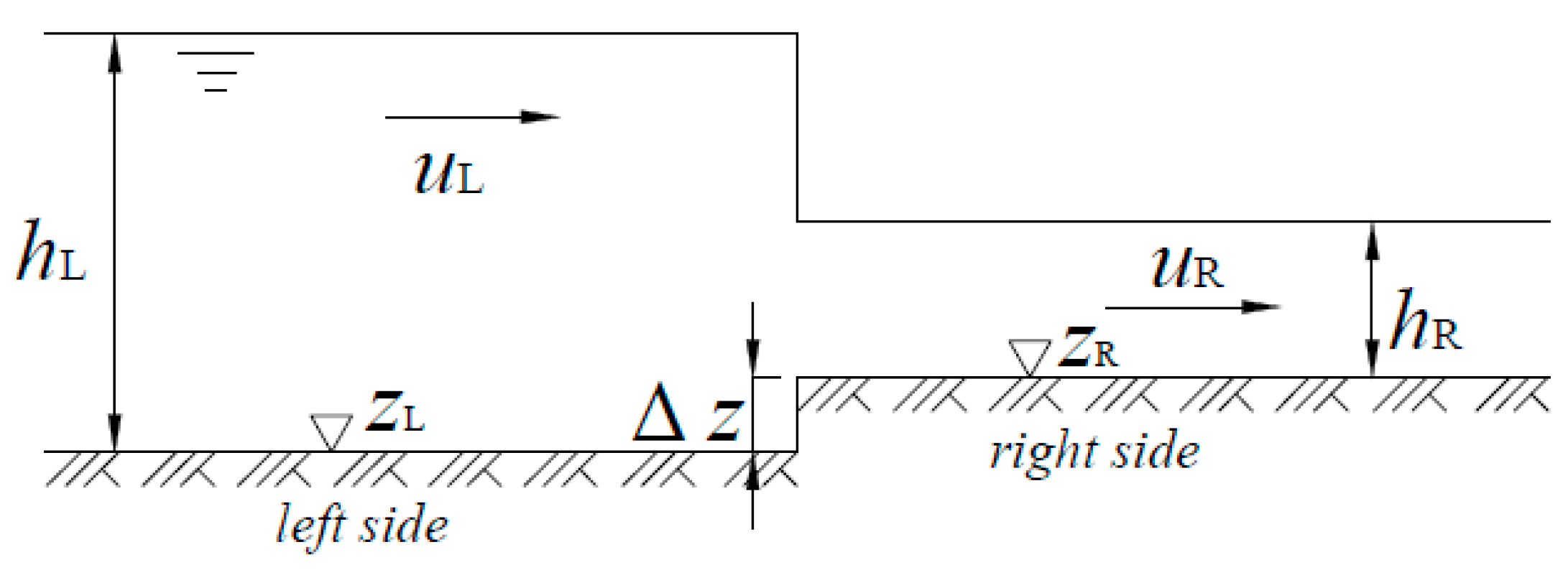
Figure 1 provides a detailed illustration of the SRP for a sudden step of height ∆z in the channel bed. Here, the bed is wet throughout the channel. Local depth, bulk velocity, and bed elevation are represented by (hL, UL, and zL) to the immediate left (upstream) of the step and (hR, UR, and zR) to the immediate right (downstream) of the step.
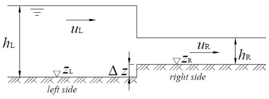
Figure 1.
Close-up view of wet-step Riemann problem at a cell interface.
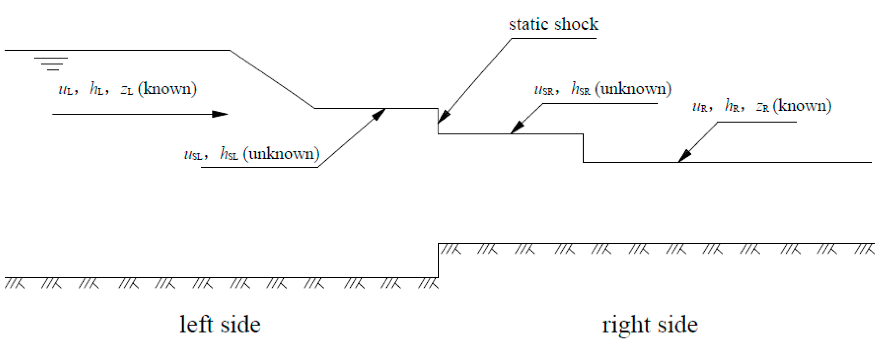
Figure 2 illustrates one of four possible Riemann solutions for the SRP. At the step, a static shock occurs with zero celerity. Immediately either side of the static shock, the variables uSL, hSL, uSR, and hSR are unknown and can be determined from relations with known variables uL, hL, zL, uR, and hR.
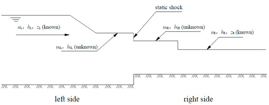
Figure 2.
Riemann solution for shallow flow over a wetted step.
If the left side is a rarefaction wave, the Riemann invariants are as follows:
If the left side is a shock-like hydraulic bore, the Riemann invariants are as follows:
where s is the speed of the shock.
If the right side is a rarefaction wave, then
If the right side is a shock, then
The static shock satisfies the following relationships:
where
Table 1 summarizes the Riemann states for the SRP.

Table 1.
Conventional equations of Riemann solver for wet-bed SRP.
3. Solution Methodology
We rewrite Equation (2) as
where
Taking the derivative of Equation (9) with respect to hSL, then
Similarly, Equation (4) is rewritten as
in which
Differentiating Equation (12) with respect to hSR yields the following:
Setting
Equation (3) becomes:
and
Combining Equations (16) and (17):
where
Substituting Equations (16) and (19) into Equation (18) gives
Rearranging,
From Equation (19):
Substituting Equation (22) into Equation (21) yields:
Based on Equation (15)
Substituting Equation (24) into Equation (21) gives:
Substituting Equation (23) into Equation (25) gives:
Differentiating Equations (9) and (26) with respect to hSL yields:
where
Similarly, for the right shock, we obtain:
and
where
Rewriting Equations (6) and (7), we have
and
where uSL is given by Equations (9) and (26), uSR is given by Equations (12) and (29), and D is given by Equation (8). Taking the derivative of Equation (32) with respect to hSL,
Differentiating Equation (32) with respect to hSR, we obtain:
where uSR is given by Equations (12) and (29), and is given by Equations (14) and (30). Differentiating Equation (34) with respect to hSL gives:
where uSL is given by Equations (9) and (26), is given by Equations (11) and (27), and . Differentiating Equation (33) with respect to hSR, we obtain
where uSR is given by Equations (12) and (29), and is given by Equations (14) and (30).
Table 2 summarizes the equations derived for the Riemann states in the SRP.
Table 2.
New equations for Riemann solver of wet-bed SRP.
In the numerical model, we use the Levenberg–Marquardt method [41] (the source code can be downloaded from the website of the Utah University) to solve for hSL and hSR by configuring the main equation and Jacobi matrix according to Table 2. Then, uSL and uSR and the wave speed are determined either side of the step.
From the menu of functions available in the original code, we choose the f02 function which is called in subroutine lmder1_test and configure it with f1 Equation (32) and f2 Equation (33) as below:
in which uls is uSL, urs is uSR, r is D, h1 is hSL, and h2 is hSR as given in Equations (32) and (33). The uls, urs and r variables are determined from Equations (8), (9), (11), (12), (14), (26), (27), (29), and (30) and the code inserted in the subroutine given in lmder1_test. The last 2 variables, h1 and h2, are unknowns that are then determined.
fvec(1) = h1*uls − h2*urs;
fvec(2) = h1*uls*uls + 0.5*g*h1*h1 − h2*urs*urs − 0.5*gr*h2*h2 − r;
4. Results
Our proposed Riemann solver for the wet-bed SRP is tested for four benchmark cases involving different combinations of rarefactions and shock-like hydraulic bores in a straight, open channel containing a sudden step. The set-up and numerical results for each case are described below.
4.1. Case 1: Rarefaction-Static Shock-Rarefaction
This first case investigates flow over a 1 m high step within an otherwise horizontal channel of total length 25 m. The step is located at the middle of the channel and extends downstream, such that the bed elevation z = 0 for x < 12.5 m and z = 1 m for x ≥ 12.5 m.
Table 3 lists the initial conditions. Please note that the initial values of hSL and hSR at x = 12.5 m are both set to 5.0 m. The converged results obtained using LM iteration are hSL = 4.39958 m, uSL = 2.576215 m/s, hSR = 2.92406 m, and uSR = 3.87621 m/s. Figure 3 compares our numerical solution obtained on a grid of 250 cells at time t = 0.79932 s with the exact analytical solution derived by Murillo and García-Navarro [42]. The agreement is excellent, except for slight discrepancies at the smoothed ends of the rarefaction waves.
Table 3.
Initial conditions for rarefaction-static shock-rarefaction.
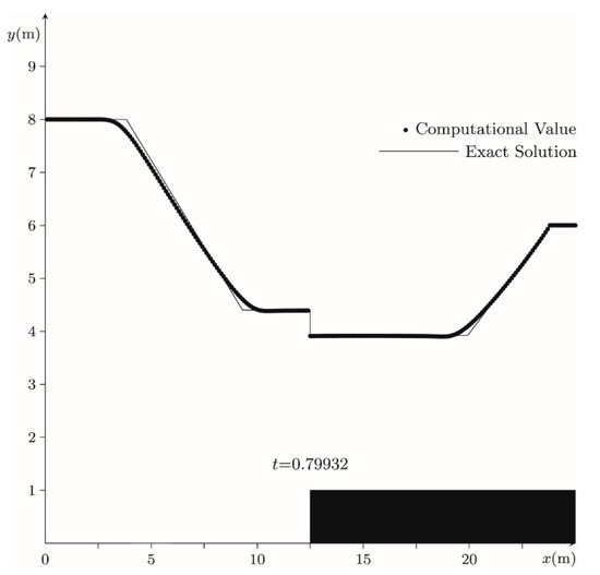
Figure 3.
Case 1: present numerical and exact [42] local free-surface elevation profiles.
4.2. Case 2: Shock-Static Shock-Shock
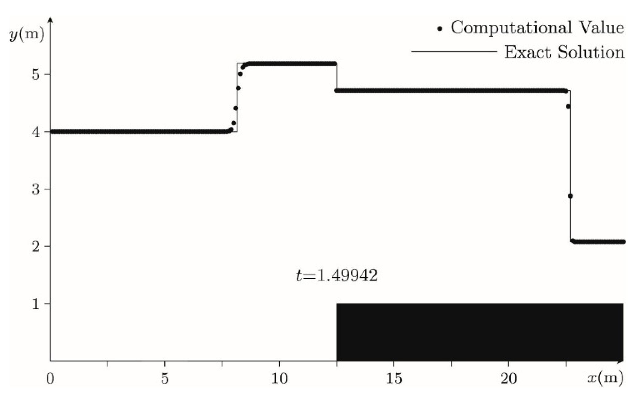
The second case examines a tidal bore encountering a river flow.
Table 4 lists the initial conditions: on the left side of the step interface, there is a flow moving to the right with a depth of 4 m and a velocity of 4.75 m/s, while on the right side, the flow moves to the left with a depth of 1.0838 m and a speed of 2.1854 m/s.
Table 4.
Initial conditions for shock-static shock-shock.
The initial values of hSL and hSR are again set to 5.0 m. After application of LM iteration, the converged results are hSL = 5.19336 m, uSL = 2.99267 m/s, hSR = 3.71648 m, and uSR = 4.18192 m/s. Figure 4 compares the converged free-surface elevation profile along the channel on a grid of 250 grid cells at time t = 1.48842 s with the exact solution obtained by Murillo and García-Navarro [42]. Again, the two solutions are almost identical, except for a slight smoothing effect on the front face of the leftward propagating bore at x~7 m.
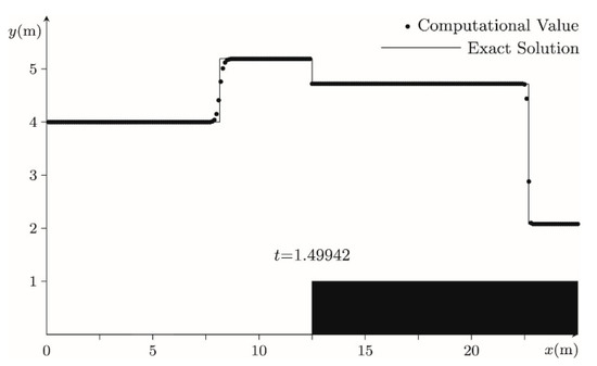
Figure 4.
Case 2: present numerical and exact [42] local free-surface elevation profiles.
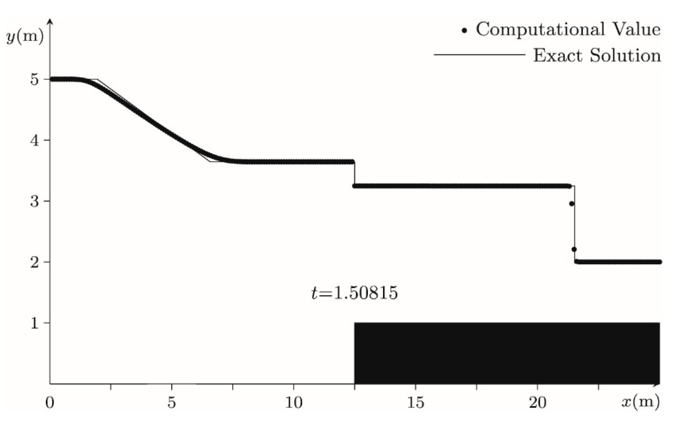
4.3. Case 3: Rarefaction-Static Shock-Shock
This scenario involves a dam-break event occurring over a wet bed, with the water in the open channel initially at rest. The channel is 25 m in length and is divided into 250 computational cells. Table 5 provides the starting flow parameters on both sides of the step interface.
Table 5.
Initial conditions for dam break in a channel with a step.
Our results converge to hSL = 3.64399 m, uSL = 2.08243 m/s, hSR = 2.24788 m, and uSR = 3.32036 m/s. Figure 5 shows the outstanding agreement obtained between the predicted profile by the present numerical scheme at t = 1.30815 s and the exact solution given by Murillo and García-Navarro [42].
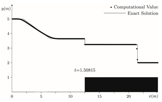
Figure 5.
Case 3: present numerical and exact [42] local free-surface elevation profiles.
4.4. Case 4: Comparison Between Present Algorithm and That of Xu et al. [38]
The foregoing classical cases do not distinguish between the present algorithm and that previously proposed by Xu et al. [38], with both algorithms giving the same results after several iterative steps, and the present method requiring 1 or 2 more steps. To examine the robustness of the new scheme, we consider the following case where hL = 0.142500 m, uL = 1.263158 m/s, hR = 0.148000 m, uR = 1.216216 m/s, and dz = 0.005500 m. We found that Xu et al.’s [38] algorithm was unable to achieve convergence whereas the present method provided the correct result: hSL = 0.14912 m, uSL = 1.20887 m/s, hSR = 0.14925 m, and uSR = 1.22638 m/s. This case demonstrates that the method proposed herein is more robust than the previous algorithm suggested by Xu et al. [38]. The exact solution given by Murillo and García-Navarro [42] is hSL = 0.14525 m, uSL = 1.263158 m/s, hSR = 0.1425 m, uSR = 1.263158 m/s.
5. Conclusions
This study has derived a pair of governing equations whose two dependent variables comprise local depths to the immediate left and right of an abrupt step in a one-dimensional wet-bed open channel. The equations are unified in representing combined shock and rarefaction conditions and are solved using the iterative Levenberg–Marquardt method. The new approach is simpler and more robust than previous methods and is demonstrated to give correct predictions of rarefaction and shock-like hydraulic bores for three classic benchmark and one realistic cases. The excellent agreement between the present model predictions and established analytical solutions demonstrates that our algorithm performs effectively over the range of cases considered herein. In future work, we intend to carry out a thorough comparison between our algorithm and previous numerical schemes in order to evaluate the relative errors and CPU run times on the same platform. It is also intended to extend the present algorithm to dry-bed cases and two-horizontal dimensions in space for the model to be applicable to more general simulations of practical engineering interest.
Author Contributions
Methodology, R.X.; Software, R.X.; Validation, R.X.; Writing—original draft, R.X.; Writing—review & editing, A.G.L.B. All authors have read and agreed to the published version of the manuscript.
Funding
This research received no external funding.
Data Availability Statement
Data is contained within the article.
Conflicts of Interest
The authors declare no conflict of interest.
References
- Abbott, M.B. Computational Hydraulics. In Elements of The Theory of Free Surface Flows; Pitman: London, UK, 1979; p. 326. [Google Scholar]
- Cunge, J.A.; Holly, F.M.; Verwey, A. Practical Aspects of Computational River Hydraulics; Pitman: London, UK, 1980; p. 416. [Google Scholar]
- Tan, W.Y. Shallow Water Hydrodynamics. In Elsevier Oceanography Series; Elsevier: Amsterdam, The Netherlands, 1992; Volume 55, p. 433. [Google Scholar]
- Bender, J.; Öffner, P. Entropy-Conservative Discontinuous Galerkin Methods for the Shallow Water Equations with Uncertainty. Commun. Appl. Math. Comput. 2024, 6, 1978–2010. [Google Scholar] [CrossRef]
- Yao, S.; Kan, G.; Liu, C.; Tang, J.; Cheng, D.; Guo, J.; Jiang, H. A Hybrid Theory-Driven and Data-Driven Modeling Method for Solving the Shallow Water Equations. Water 2023, 15, 3140. [Google Scholar] [CrossRef]
- Li, L.; Wang, Z.; Zhao, Z.; Zhu, J. A new high order hybrid WENO scheme for hyperbolic conservation laws. Numer. Methods Partial. Differ. Equ. 2023, 39, 4347–4376. [Google Scholar] [CrossRef]
- Zhang, Z.; Zhou, X.; Li, G.; Qian, S.; Niu, Q. A New Entropy Stable Finite Difference Scheme for Hyperbolic Systems of Conservation Laws. Mathematics 2023, 11, 2604. [Google Scholar] [CrossRef]
- Zahran, Y.H.; Abdalla, A.H. Central random choice methods for hyperbolic conservation laws. Ric. Di Mat. 2022, 73, 2091–2130. [Google Scholar] [CrossRef]
- Fu, L.; Hu, X.Y.; Adams, N.A. A family of high-order targeted ENO schemes for compressible-fluid simulations. J. Comput. Phys. 2016, 305, 333–359. [Google Scholar] [CrossRef]
- Liang, T.; Fu, L. A new type of non-polynomial based TENO scheme for hyperbolic conservation laws. J. Comput. Phys. 2023, 497, 112618. [Google Scholar] [CrossRef]
- Deng, X.; Jiang, Z.-H.; Yan, C. Efficient ROUND schemes on non-uniform grids applied to discontinuous Galerkin schemes with Godunov-type finite volume sub-cell limiting. J. Comput. Phys. 2025, 522, 113575. [Google Scholar] [CrossRef]
- Leveque, R.J. Large Time Step Shock-Capturing Techniques for Scalar Conservation Laws. SIAM J. Numer. Anal. 1982, 19, 1091–1109. [Google Scholar] [CrossRef]
- Murillo, J.; García-Navarro, P.; Brufau, P.; Burguete, J. Extension of an explicit finite volume method to large time steps (CFL>1): Application to shallow water flows. Int. J. Numer. Methods Fluids 2006, 50, 63–102. [Google Scholar] [CrossRef]
- Morales-Hernandez, M.; García-Navarro, P.; Murillo, J. A large time step 1D upwind explicit scheme (CFL> 1): Application to shallow water equations. J. Comput. Phys. 2012, 231, 6532–6557. [Google Scholar] [CrossRef]
- Morales-Hernández, M.; Hubbard, M.E.; García-Navarro, P. A 2D extension of a Large Time Step explicit scheme (CFL>1) for unsteady problems with wet/dry boundaries. J. Comput. Phys. 2014, 263, 303–327. [Google Scholar] [CrossRef]
- Morales-Hernández, M.; Lacasta, A.; Murillo, J.; García-Navarro, P. A Large Time Step explicit scheme (CFL>1) on unstructured grids for 2D conservation laws: Application to the homogeneous shallow water equations. Appl. Math. Model. 2017, 47, 294–317. [Google Scholar] [CrossRef]
- Xu, R.; Zhong, D.; Wu, B.; Fu, X.; Miao, R. A Large Time Step Godunov Scheme for Free-surface Shallow Water Equations. Chin. Sci. Bull. 2014, 59, 2534–2540. [Google Scholar] [CrossRef]
- Qian, Z.; Lee, C.-H. A class of large time step Godunov schemes for hyperbolic conservation laws and applications. J. Comput. Phys. 2011, 230, 7418–7440. [Google Scholar] [CrossRef]
- Dong, H.; Liu, F. Large time step wave adding scheme for systems of hyperbolic conservation laws. J. Comput. Phys. 2018, 374, 331–360. [Google Scholar] [CrossRef]
- Liu, F.; Dong, H. Second-order large time step wave adding scheme for hyperbolic conservation laws. J. Comput. Phys. 2020, 408, 109279. [Google Scholar] [CrossRef]
- Lindqvist, S.; Aursand, P.; Flåtten, T.; Solberg, A.A. Large Time Step TVD Schemes for Hyperbolic Conservation Laws. SIAM J. Numer. Anal. 2016, 54, 2775–2798. [Google Scholar] [CrossRef]
- Prebeg, M.; Flåtten, T.; Müller, B. Large Time Step Roe scheme for a common 1D two-fluid model. Appl. Math. Model. 2017, 44, 124–142. [Google Scholar] [CrossRef]
- Harten, A. On a Large Time-Step High Resolution scheme. Math. Comput. 1986, 46, 379–399. [Google Scholar] [CrossRef]
- Xu, R.; Borthwick, A.G.L.; Xu, B. Application of Large Time Step TVD High Order Scheme to Shallow Water Equations. Atmosphere 2022, 13, 1856. [Google Scholar] [CrossRef]
- Qian, Z.; Lee, C.-H. On large time step TVD scheme for hyperbolic conservation laws and its efficiency evaluation. J. Comput. Phys. 2012, 231, 7415–7430. [Google Scholar] [CrossRef]
- García-Navarro, P.; Cendón, E.V. On numerical treatment of the source terms in the shallow water equations. Comput. Fluids 2000, 29, 951–979. [Google Scholar] [CrossRef]
- Rogers, B.D.; Borthwick, A.G.; Taylor, P.H. Mathematical balancing of flux gradient and source terms prior to using Roe’s approximate Riemann solver. J. Comput. Phys. 2003, 192, 422–451. [Google Scholar] [CrossRef]
- Liang, Q.; Borthwick, A.G. Adaptive quadtree simulation of shallow flows with wet-dry fronts over complex topography. Comput. Fluids 2009, 38, 221–234. [Google Scholar] [CrossRef]
- Zhang, Z.; Duan, J.; Tang, H. High-order accurate well-balanced energy stable adaptive moving mesh finite difference schemes for the shallow water equations with non-flat bottom topography. J. Comput. Phys. 2023, 492, 112451. [Google Scholar] [CrossRef]
- Alcrudo, F.; Benkhaldounb, F. Exact solutions to the Riemann problem of the shallow water equations with a bottom step. Comput. Fluids 2001, 30, 643–671. [Google Scholar] [CrossRef]
- Bukreev, V.I.; Gusev, A.V.; Ostapenko, V.V. Breakdown of a discontinuity of the free fluid surface over a bottom step in a channel. Fluid Dyn. 2003, 38, 889–899. [Google Scholar] [CrossRef]
- Gallouët, T.; Hérard, J.-M.; Seguin, N. Some Approximate Godunov schemes to compute shallow-water equations with topography. Comput. Fluids 2003, 32, 479–513. [Google Scholar] [CrossRef]
- Chinnayya, A.; LeRoux, A.Y.; Seguin, N. A well-balanced numerical scheme for the approximation of the shallow-water equations with topography: The resonance phenomenon. Int. J. Finite Vol. 2004, 1, 1–33. [Google Scholar]
- Andrianov, N. Performance of numerical methods on the non-unique solution to the Riemann problem for the shallow water equations. Int. J. Num. Methods Fluids 2005, 47, 825–831. [Google Scholar] [CrossRef]
- Aleksyuk, A.I.; Belikov, V.V. The uniqueness of the exact solution of the Riemann problem for the shallow water equations with discontinuous bottom. J. Comput. Phys. 2019, 390, 232–248. [Google Scholar] [CrossRef]
- Aleksyuk, A.I.; Malakhov, M.A.; Belikov, V.V. The exact Riemann solver for the shallow water equations with a discontinuous bottom. J. Comput. Phys. 2022, 450, 110801. [Google Scholar] [CrossRef]
- Bernetti, R.; Titarev, V.; Toro, E. Exact solution of the Riemann problem for the shallow water equations with discontinuous bottom geometry. J. Comput. Phys. 2008, 227, 3212–3243. [Google Scholar] [CrossRef]
- Xu, R.; Borthwick, A.G.; Ma, H.; Xu, B. Godunov-type large time step scheme for shallow water equations with bed-slope source term. Comput. Fluids 2022, 233, 105222. [Google Scholar] [CrossRef]
- Rosatti, G.; Begnudelli, L. The Riemann Problem for the one-dimensional, free-surface Shallow Water Equations with a bed step: Theoretical analysis and numerical simulations. J. Comput. Phys. 2010, 229, 760–787. [Google Scholar] [CrossRef]
- Toro, E.F. Riemann Solvers and Numerical Methods for Fluid Dynamics. In A Practical Introduction, 3rd ed.; Springer: Berlin/Heidelberg, Germany, 2009. [Google Scholar]
- Dold, A.; Eckmann, B. The Levenberg-Marquardt algorithm Implementation and theory. In Lecture Notes in Mathematics; Springer: Berlin/Heidelberg, Germany, 1977. [Google Scholar]
- Murillo, J.; García-Navarro, P. Weak solutions for partial differential equations with source terms: Application to the shallow water equations. J. Comput. Phys. 2010, 229, 4327–4368. [Google Scholar] [CrossRef]

Disclaimer/Publisher’s Note: The statements, opinions and data contained in all publications are solely those of the individual author(s) and contributor(s) and not of MDPI and/or the editor(s). MDPI and/or the editor(s) disclaim responsibility for any injury to people or property resulting from any ideas, methods, instructions or products referred to in the content. |
© 2025 by the authors. Licensee MDPI, Basel, Switzerland. This article is an open access article distributed under the terms and conditions of the Creative Commons Attribution (CC BY) license (https://creativecommons.org/licenses/by/4.0/).