Abstract
This study aimed to compare linear and non-linear regional flood frequency analysis (RFFA) models where streamflow data of 88 catchments of New South Wales (NSW), Australia, were utilized. The Quantile Regression Technique (QRT) was selected as the linear model and an Artificial Neural Network (ANN) as the non-linear model. Six different flood quantiles were considered, which are annual exceedance probabilities of 1 in 2 (Q2), 1 in 5 (Q5), 1 in 10 (Q10), 1 in 20 (Q20), 1 in 50 (Q50), and 1 in 100 (Q100). The selected two RFFA models were compared using a split-sample validation technique (70% data for training and 30% data for testing) and several statistical indices like relative error (RE), absolute median relative error (REr), bias, the median ratio of the predicted and observed flood quantiles (Qr), and the root mean square error (RMSE). The ANN model exhibited smaller bias values for Q2, Q5, Q20, and Q50 and smaller Qr values for Q10, Q20, and Q50. The REr values for the ANN model were found to be lower for smaller return periods (Q2, Q5, and Q10). The overall REr value considering all six AEPs for the ANN model is 35%, which is 37% for the QRT model. The results of this study could assist to select a suitable RFFA technique for design application in the study area.
1. Introduction
In recent years, flood damage has noticeably increased worldwide [1]. Floods affect many people globally each year [2]. Flood damage can be reduced by building flood-safe infrastructure using a risk-based approach. A design flood/flood quantile is used in this risk-based design [3]. A streamflow associated with a specific annual exceedance probability (AEP) or return period is called a design flood or flood quantile. For a gauged catchment having sufficiently long recorded flood data, at-site flood frequency analysis (FFA) is generally adopted to estimate design floods [4,5]. However, FFA is not directly applicable to ungauged catchments due to a lack of recorded flood data at the location of interest. Regional flood frequency analysis (RFFA) is one of the most widely adopted methods for ungauged catchments. In RFFA, flood-related information is conveyed from a group of gauged catchments to ungauged ones on the assumption of catchment similarity [6,7].
In RFFA, several linear methods have previously been applied such as the probabilistic rational method (PRM) [8,9], the index flood method (IFM) [10,11], the quantile regression technique (QRT) [12,13], kriging [14,15], and the generalized additive model (GAM) [16,17]. The PRM is an approximate method for estimating design floods for small- to medium-sized catchments [18]. The PRM was the recommended technique for design flood estimation at ungauged catchments in the 3rd edition of the Australian Rainfall and Runoff (ARR) guideline (ARR 1987) [19]. However, Rahman et al. [9] noted that the flood quantile estimates derived from PRM has no uncertainty measure. The IFM method relies on the identification of homogeneous regions (e.g., using Hosking and Wallis criteria) [20]. Application of the IFM was unsuccessful for Australia since homogeneous regions could not be identified [21]. The QRT may not need a perfect homogeneous region like the IFM as noted by Haddad and Rahman [22]. The QRT develops regression equations where a flood quantile is considered as a dependent variable and the chosen catchment characteristics as independent variables. The United States Geological Survey recommended the QRT for RFFA in the 1960s [23]. Rahman et al. [24] compared the QRT and the parameter regression technique (PRT) using independent component (IC) regression based on data from 88 catchments in New South Wales (NSW), Australia. The QRT with four predictors performed better than the PRT with all the ICs as predictor variables [24].
The PRM, QRT, and IFM all are dependent on linearity assumptions, which are hardly satisfied in hydrological situations, as rainfall runoff is a fundamentally non-linear process [25]. Recently, Artificial Intelligence (AI)-based techniques have shown a better performance in simulating non-linear problems [26]. Different AI-based techniques were tested based on regionalisation, e.g., an artificial neural network (ANN) [27,28], support vector regression (SVR) [29,30], gene expression programming (GEP) [31,32], an adaptive fuzzy inference system (ANFIS) [33,34], random forest (RF) [35,36,37], and Extreme Gradient Boosting (XGB) [38,39].
A number of ANN-based RFFA techniques provided accurate design flood estimates as noted below. Dawson et al. [28] showed that ANNs could provide more accurate design flood estimates than the IFM. Filipova et al. [40] used catchment and flood data of over 4000 catchments in the USA and found that an ANN model with one hidden layer provided a similar performance as complex multi-layered ANN models. Aziz et al. [41] utilised data from 452 gauged catchments across eastern Australia to develop an ANN model and conducted a comparative analysis against the QRT. The study concluded that the ANN model demonstrated superior performance over the QRT model when limited to two predictor variables.
Given the inherently non-linear nature of the rainfall-runoff process, traditional linear RFFA methods often fall short in delivering accurate design flood estimates when compared to non-linear approaches such as ANNs. Despite this, there is a noticeable lack of comprehensive studies directly comparing linear and non-linear RFFA methods within the Australian context. Notably, the current ARR guidelines continue to recommend regression-based linear RFFA techniques for general application. This study aims to address this gap by evaluating and comparing the performance of linear and non-linear RFFA methods specifically for New South Wales (NSW), Australia. The findings are expected to enhance understanding of regional flood behaviour in NSW and support the development of more robust and precise RFFA models. Ultimately, this work could inform future updates to the ARR guidelines by incorporating improved non-linear methodologies for flood estimation.
2. Study Area and Data Selection
New South Wales (NSW) state in Australia was chosen for this research as it has better quality streamflow data as compared to other Australian states. A total of 88 gauged catchments were chosen in this research, which were unaffected by major regulation (like reservoir/dam) and land use changes. Generally, about 20-year-long streamflow data are needed from each station in a region to carry out meaningful RFFA [42]. The AMF data length ranges from 25 to 89 years for the selected catchments.
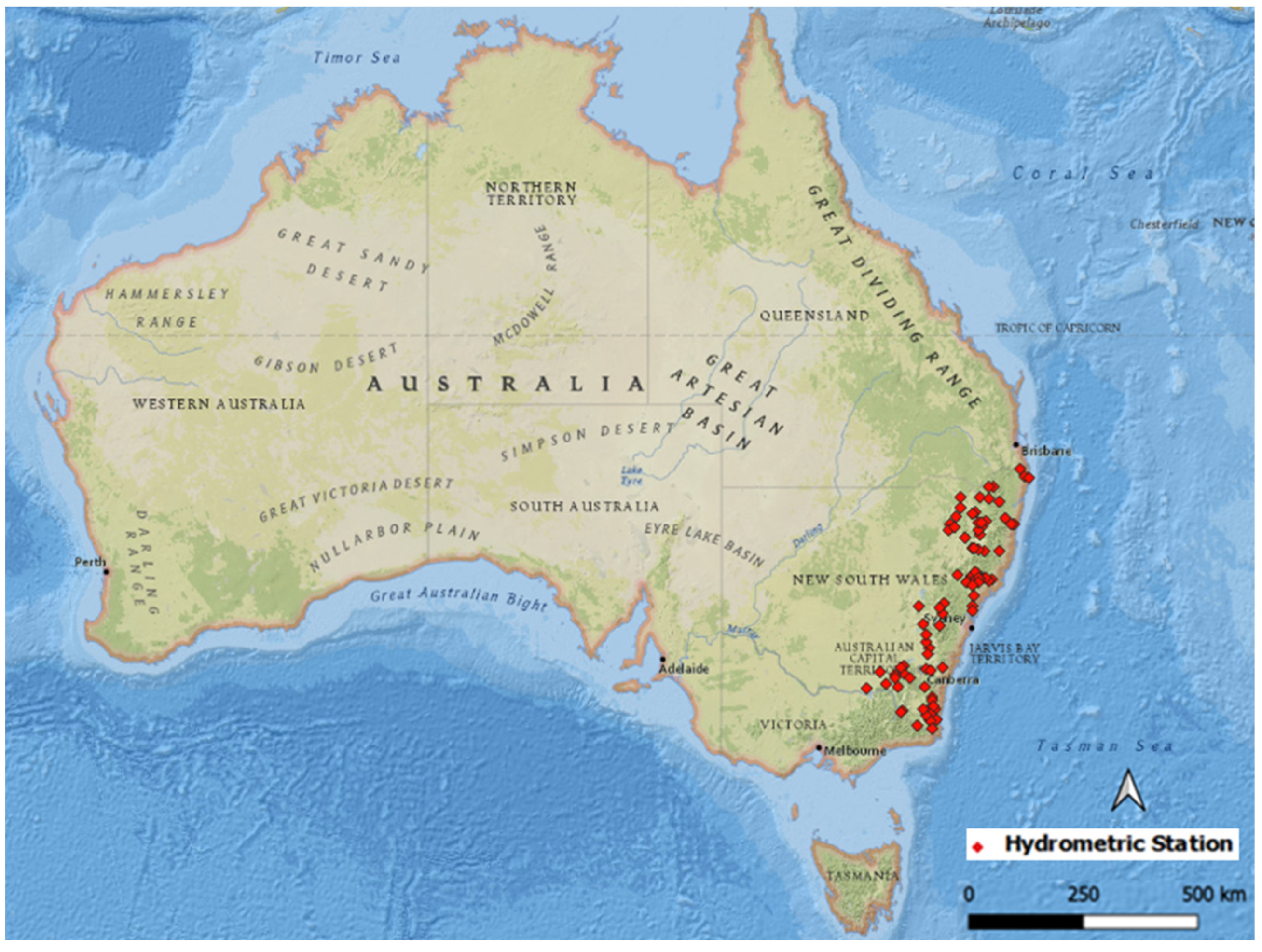
Figure 1 shows the location of the study sites. Log-Pearson Type 3 (LP3) distribution was adopted to carry out FFA using the annual maximum flood (AMF) data of the chosen sites, since LP3 usually provides more accurate quantile estimates [42]. For FFA, FLIKE 2019 software [4] was used. Design floods/flood quantiles for six AEPs were estimated, which are 1 in 2, 1 in 5, 1 in 10, 1 in 20, 1 in 50, and 1 in 100 (denoted by Q2, Q5, Q10, Q20, Q50, and Q100, respectively).

Figure 1.
Location of 88 selected sites.
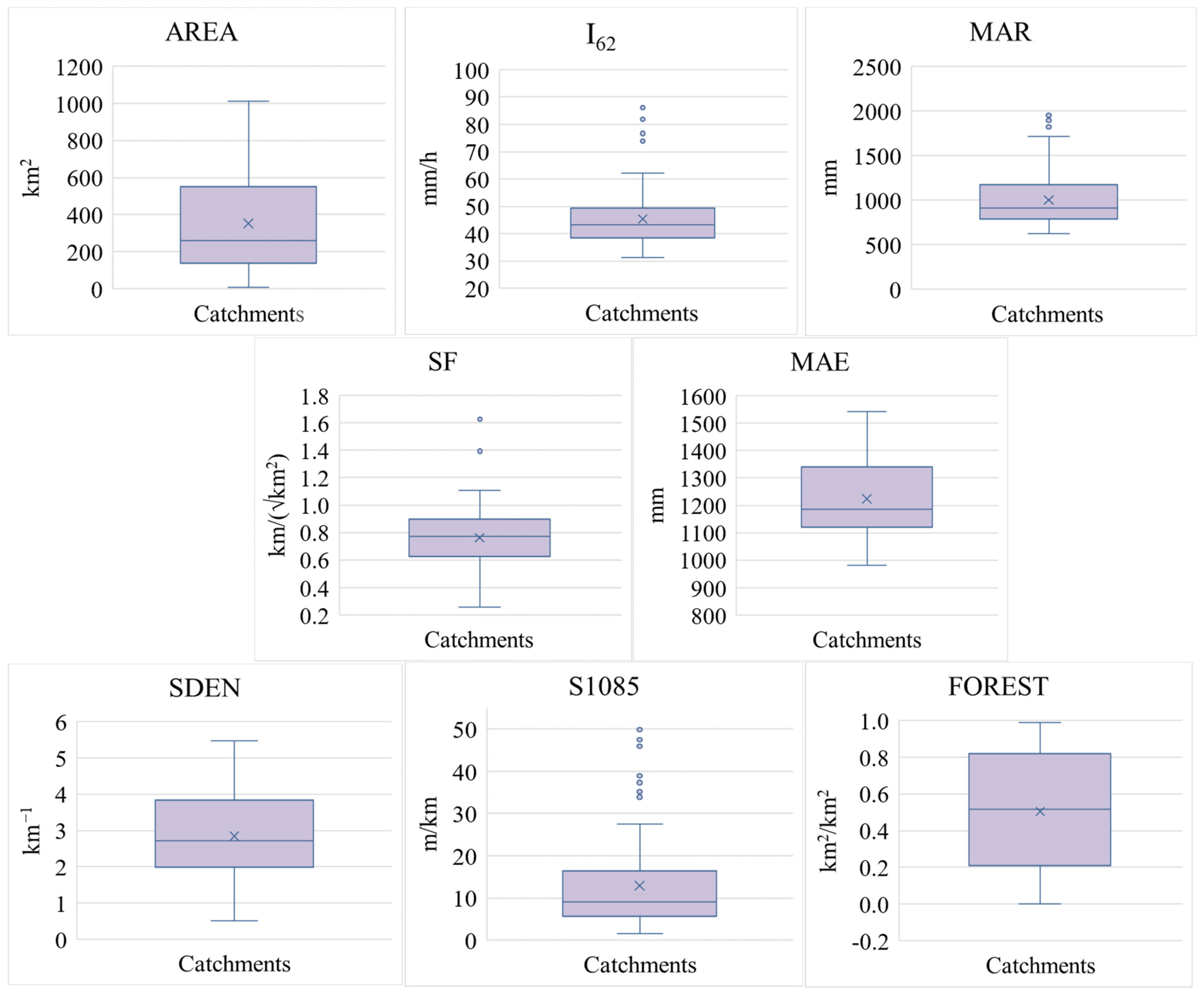
In an RFFA study, the selection of climatic and catchment characteristics (predictor variables) is an important step. Several previous studies used eight catchment characteristics to develop RFFA models for southeast Australia [41,43], as shown in Table 1. These were also adopted in this study.

Table 1.
Summary data of the chosen catchment characteristics.
The data for AREA, I62. MAR, and MAE were collected from the Australian Government website. The data of SF, SDEN, S1085, and FOREST were obtained from 1:100,000 topographic maps as explained in Rahman et al. [24]. Table 1 summarises these data and Figure 2 shows boxplots of the selected catchment characteristics for the selected 88 stations.
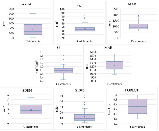
Figure 2.
Boxplots of selected catchment characteristics for the selected 88 stations.
Catchment characteristics are often correlated [22]. The correlations could be either positive or negative. Table 2 presents correlation coefficients among the predictor variables. It may be noted from Table 2 that I62, MAR, and MAE are highly correlated. SDEN is moderately correlated with I62, MAR, and MAE, whereas FOREST has moderate correlations with I62, MAR, and S1085. With AREA, all other predictors are negatively correlated, and among them, MAR and S1085 show a moderate correlation. SF shows a very low correlation with other predictors.
Table 2.
Correlation coefficient of the selected catchment characteristics for the 88 stations.
3. Methodology
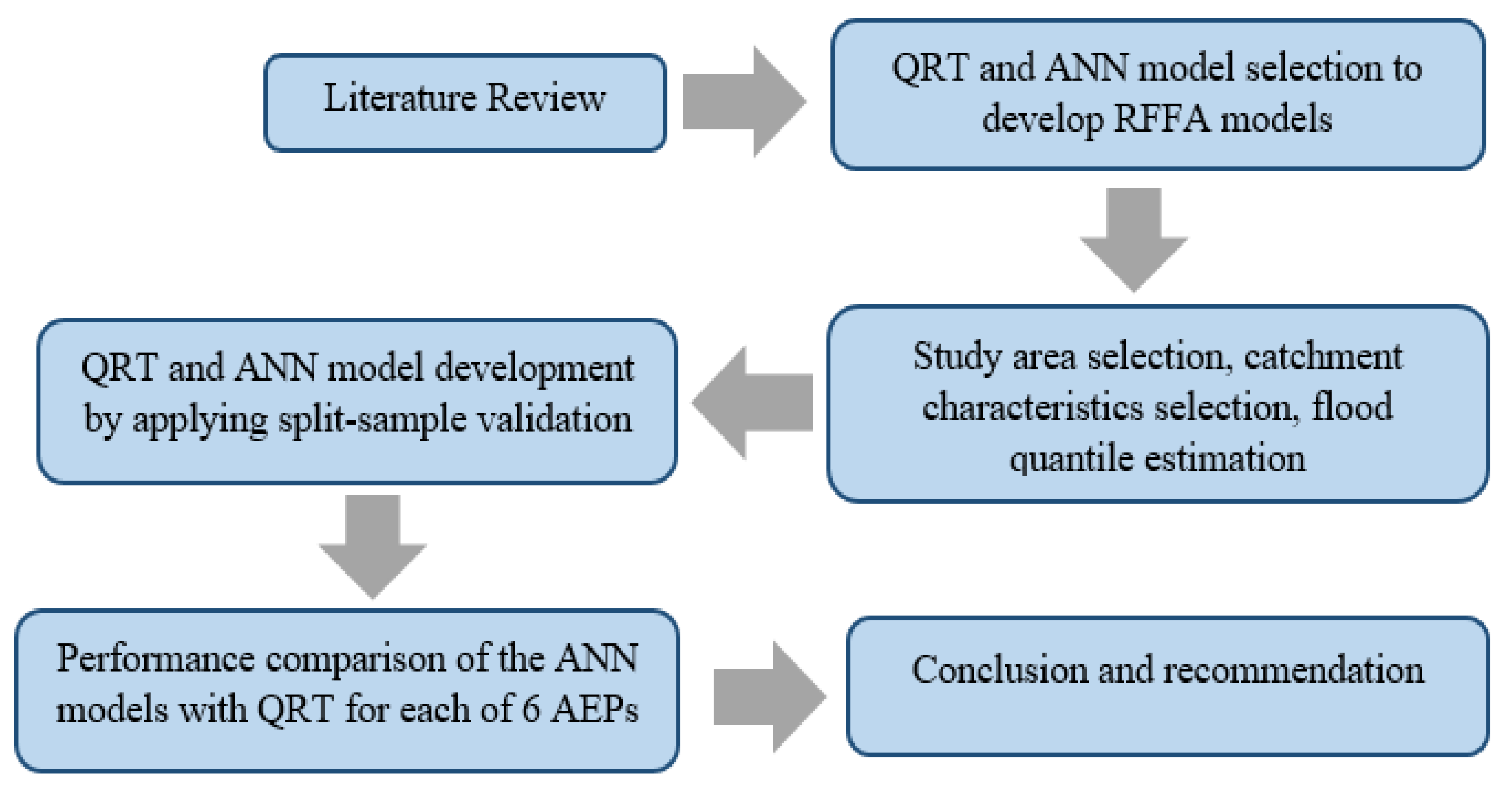
In this study, the adopted overall methodology is illustrated in Figure 3. In the beginning, the exploration of previous RFFA studies helped to understand assumptions associated with different RFFA methods. Then, the 88 hydrometric stations were selected from NSW, Australia. Streamflow data were checked for inconsistency and gaps, and catchment data (Table 1) were extracted. Afterwards, both the dependent and independent variables were log-transformed to develop the QRT, which makes the prediction equations more suitable for handling skewed data.
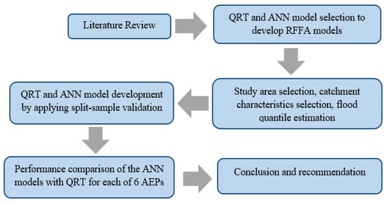
Figure 3.
Methodology adopted in this study.
This study adopted the ANN and the QRT models since these are the most widely used non-linear and linear models for RFFA, respectively. Separate ANN and QRT models were developed for each of the six return periods. The models were tested by implementing a split-sample validation (70% data for training and 30% data for testing). In the split-sample validation technique, the dataset was divided randomly for training and testing. It should be noted that other validation methods such as Mote Carlo cross-validation, as explained by Haddad et al. [44], could be applied. For the ANN model, hyperparameters were maintained as mentioned in Section 3.2. Finally, the results of both the models were compared by applying five statistical measures (presented in Section 3.3). The two RFFA models (QRT and ANN) adopted in this study are explained below.
3.1. QRT
In the QRT, an estimation model is formulated by regressing a flood quantile (e.g., Q2) with a set of catchment characteristics.
The general form of the equation is as follows:
Here, QT = flood discharge for a given AEP of 1 in T, the independent variables X = (X1, X2, …, X8), and the regression coefficients are β0, β1, β2, …, β8. The regression coefficients can be estimated by several techniques; however, the ordinary least-squares (OLS) method is one of the commonly adopted methods.
3.2. ANN
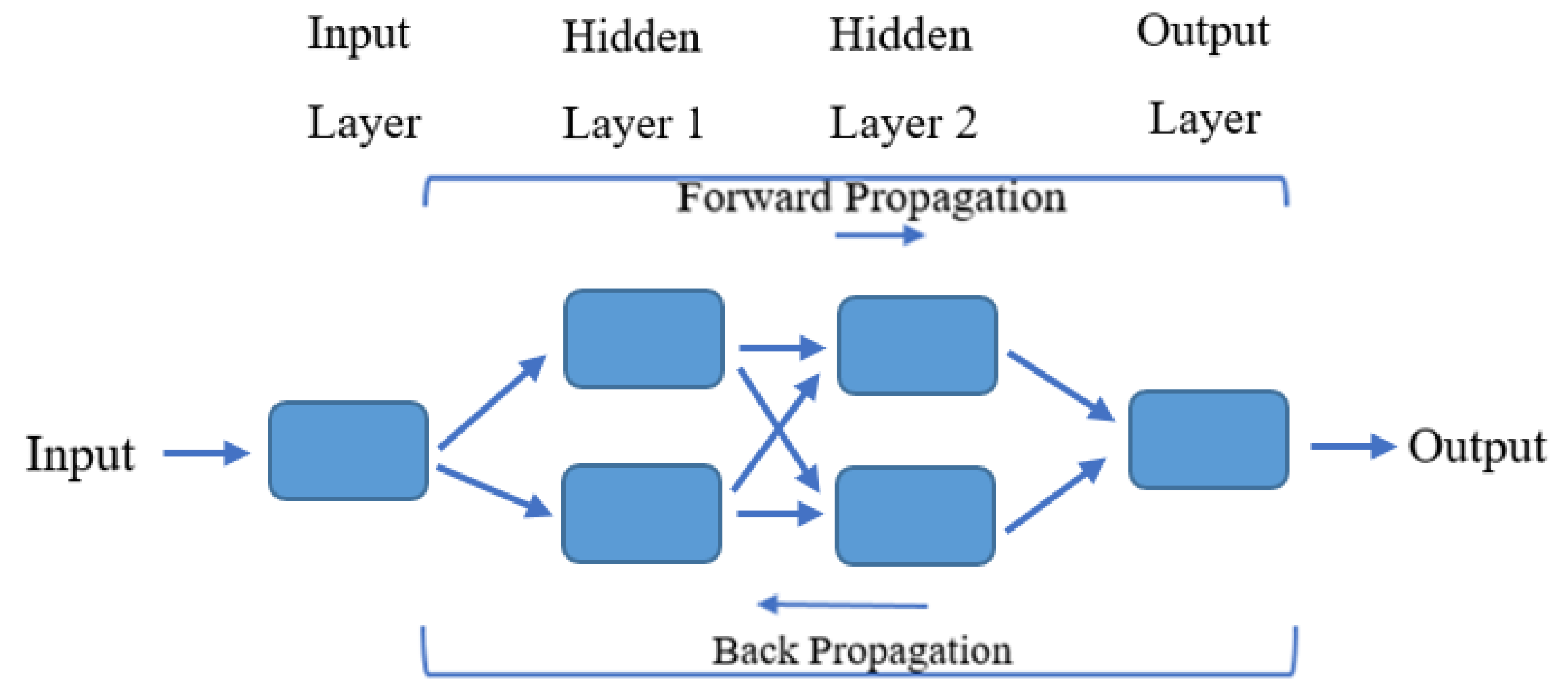
The concept of artificial neural networks (ANNs) originates from the functioning of biological neural systems. McCulloch and Pitts [45] proposed a mathematical formulation of the very first ANN model. ANN architectures can vary, including single-layer, double-layer, and multilayer designs. In a multilayer network, the first component is the input layer, followed by one or more hidden layers, and concluding with the output layer. Each layer has a connection to the following or the same layer nodes depending on the model type. Two nodes are connected via a weight connection network and an activation function, which stimulate the neuron initially. Information flows from the input layer through the hidden layer(s) and ultimately reaches the output layer, which is called forward propagation. The ANN model makes predictions by manipulating model parameters and weights by using a backpropagation (BP) process [46]. Figure 4 shows the concept of the multilayer ANN model. ANN model overfitting is related to the model architecture and the number of data points used in the model training. In this study, an ANN learning rate of 0.01 and maximum iterations of 1001 were adopted. The number of hidden layers maintained is 3–5 so that the model does not suffer from overfitting [47,48,49]. As the activation function, a Rectified Linear Unit (ReLU) was adopted to create a non-linearity aspect to the ANN model.
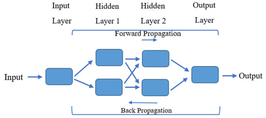
Figure 4.
Multilayer ANN model concept.
3.3. Statistical Indices
Several statistical indices (Equations (1)–(6)) were utilized for evaluating the developed RFFA techniques. Both the observed and estimated flood quantiles were log-transformed by calculating the root mean square error (RMSE) and bias. The reason behind using log-transformed flood quantiles is to reduce the influence by the large flood peaks in modelling [50]. In finding the relative error percentage (RE), median absolute relative error (REr) and Qr ratio, observed flood quantiles (Qobs) and predicted flood quantiles (Qpred) are adopted. For all the statistical measures, the lowest values are preferred except the Qr where the preferred value is 1.00.
Here, for the test catchments, Qobs is the observed flood quantile from FFA, and Qpred is the predicted flood quantile for the test catchment, obtained from the developed prediction equation based on the QRT and ANN.
4. Results
Table 3 provides the REr, bias, and median Qr values for the QRT and ANN models (based on 27 test catchments). Table 3 reveals that the ANN model outperforms the QRT model in terms of REr for Q2, Q5, and Q10, bias for Q2, Q5, Q20, and Q50, and median Qr for Q10, Q20, and Q50. The overall median REr considering all the six AEPs for the ANN model is 35.45% (which is 37.44% for the QRT). The overall median bias for the ANN model (0.026) is much smaller than that for the QRT model (−0.050). Furthermore, the overall Qr value for the ANN model is closer to the ideal value of 1.00 than that of the QRT model. It should be noted here that none of the two models performed equally well (Table 3) across all the six AEPs and the three statistical indices.
Table 3.
Three statistical measures for the two models (QRT and ANN).
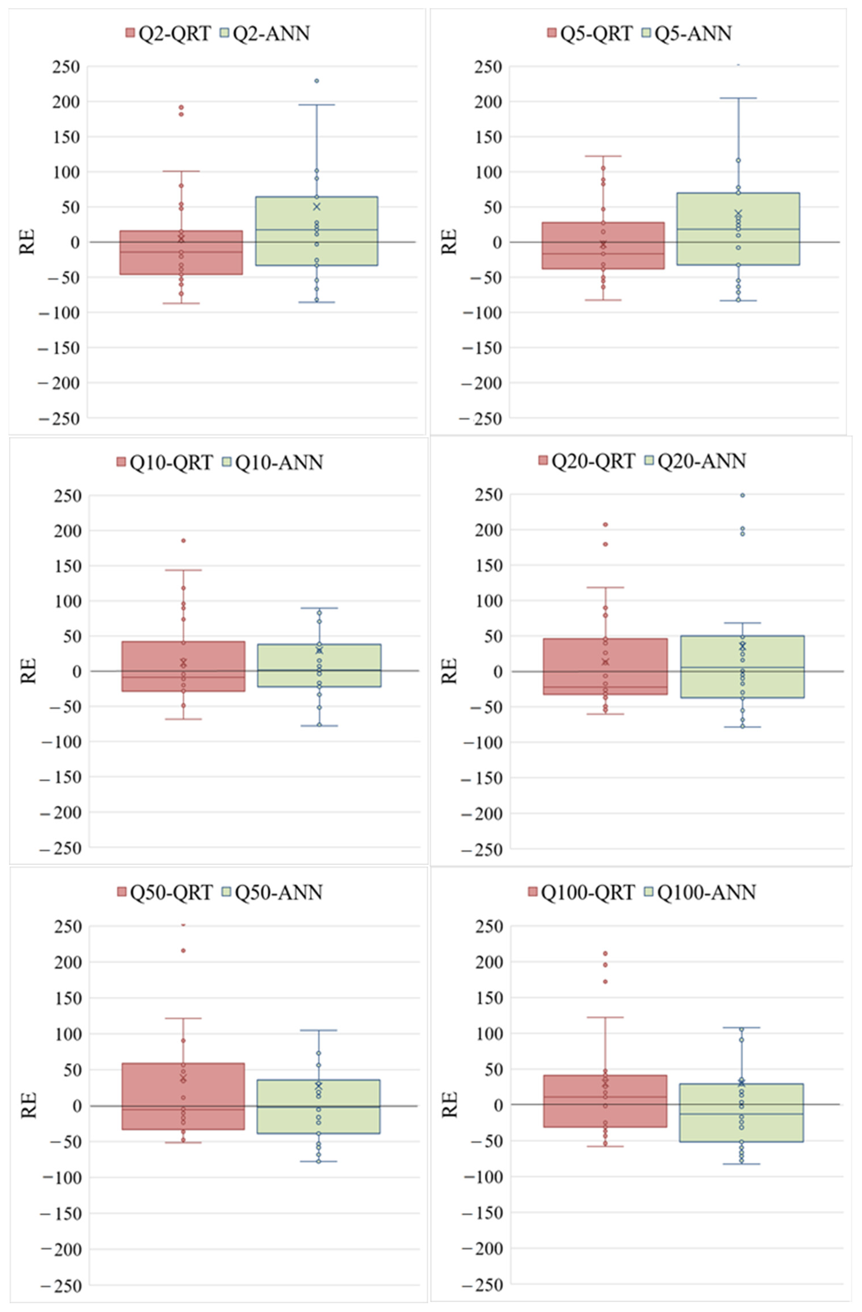
Figure 5 shows RE box plots associated with the QRT and ANN models for the six AEPs. For the ANN model, the box widths for Q10, Q20, and Q50 are narrower than those for the QRT. In relation to bias, the ANN performs better for Q10, Q20, and Q50 than does the QRT. For Q100, the box width is very similar for both the models, and for Q2 and Q50, the box width for the QRT model is much narrower than that for the ANN model. In terms of bias, the ANN model provides very good results (where the 0-0 reference line very well aligns with the median value, represented by the solid line with the box).
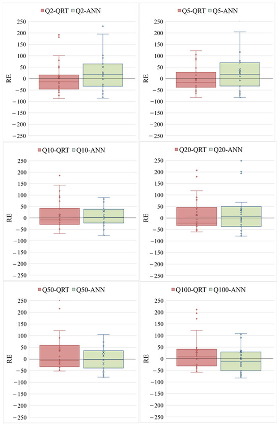
Figure 5.
Boxplot of RE values associated with QRT and ANN models.
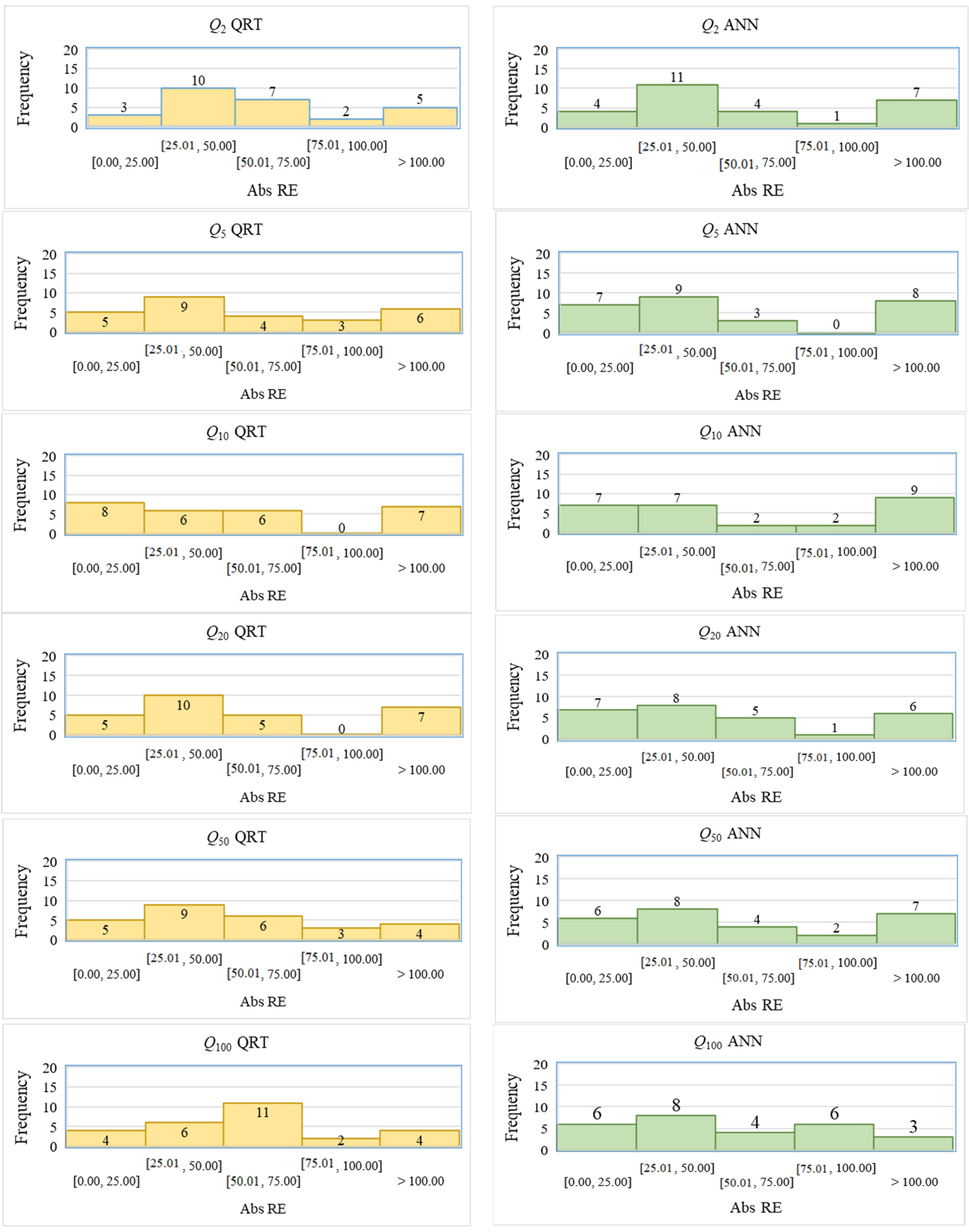
Figure 6 represents histograms of the Abs RE values associated with the QRT and ANN models. This figure shows that for the ANN model, the number of stations with Abs RE values less than 25% is higher for all the AEPs except Q2. However, the ANN shows a higher number of stations with Abs RE values more than 100% for Q2, Q5, and Q20 compared to the QRT model. These results show that generally, the ANN model outperforms the QRT model by producing smaller values of the Abs RE for most of the stations. It should be noted that for a few catchments, the ANN model did not perform well, resulting in higher Abs RE values. It would be necessary to carry out further study to find out the reason for this poorer performance.
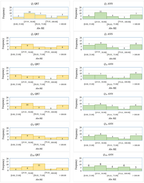
Figure 6.
Histogram of Abs RE values in QRT and ANN for six AEPs.
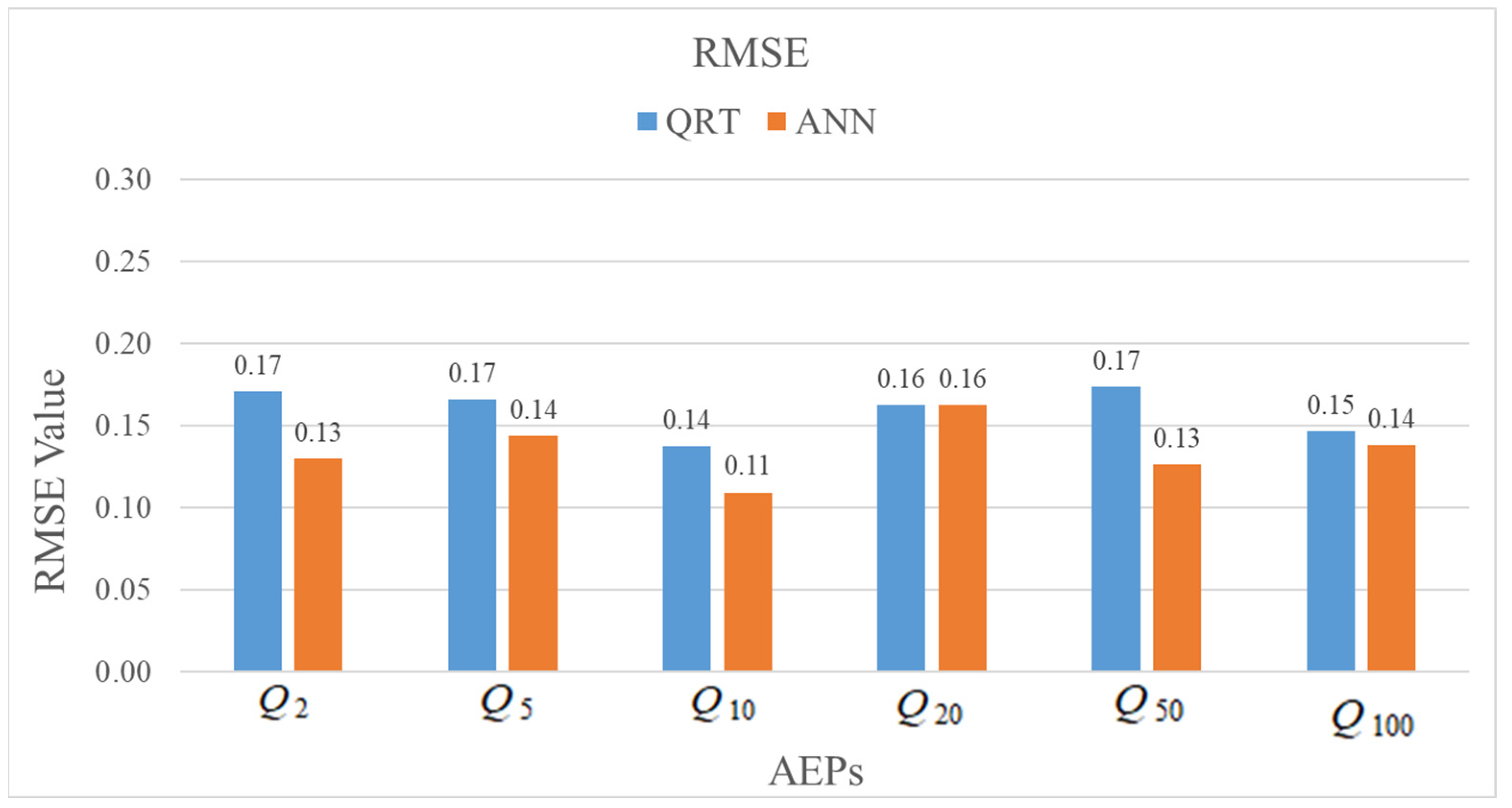
Figure 7 presents the RMSE bar plot for the QRT and ANN models, which shows that the ANN produces smaller RMSE values for all the AEPs except the Q20. For Q20, both the models show similar RMSE values
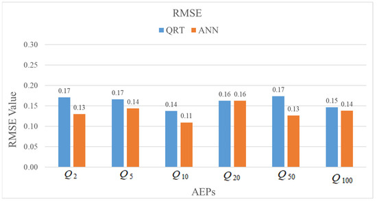
Figure 7.
RMSE bar plot for QRT and ANN models for six AEPs.
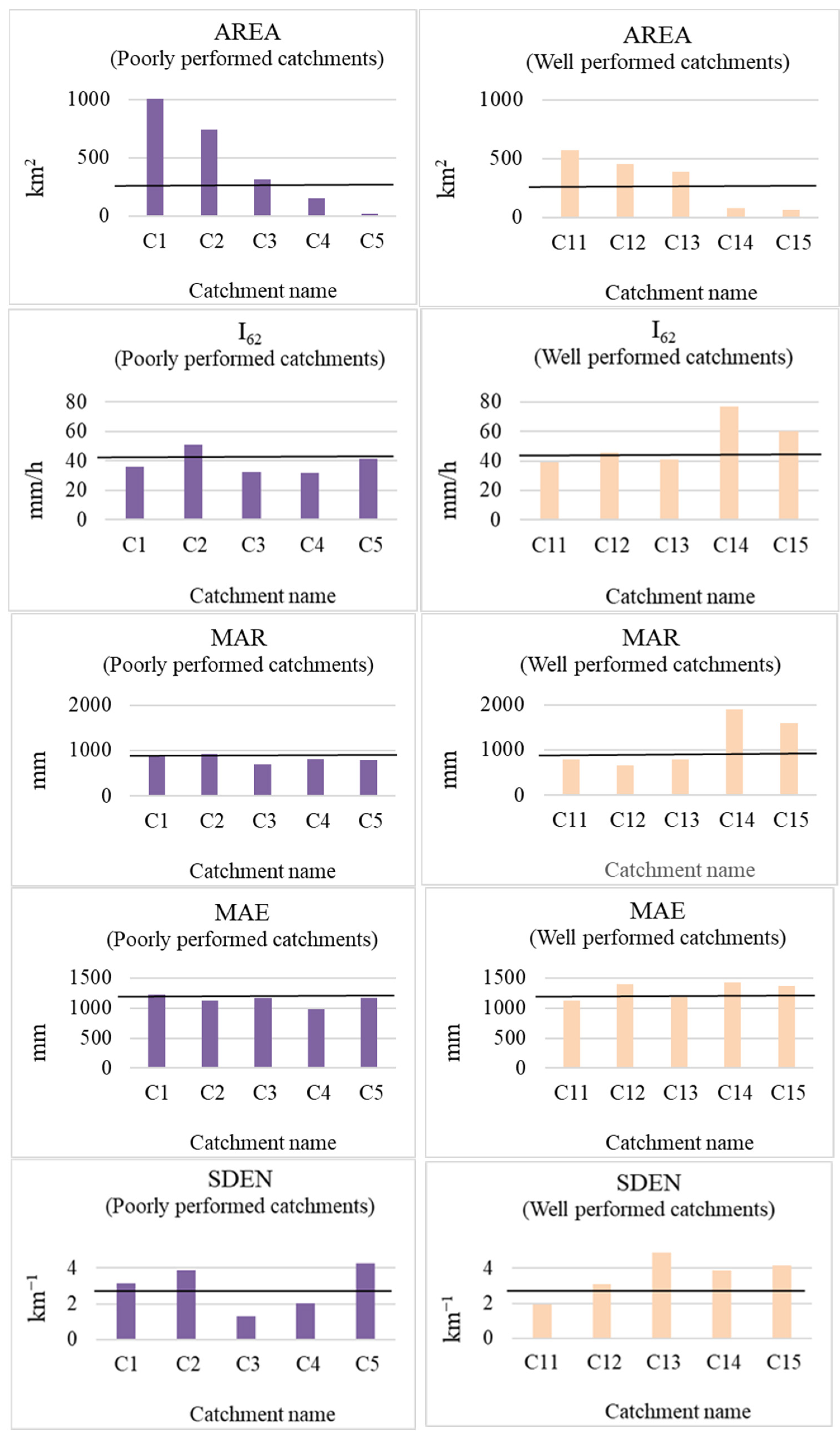
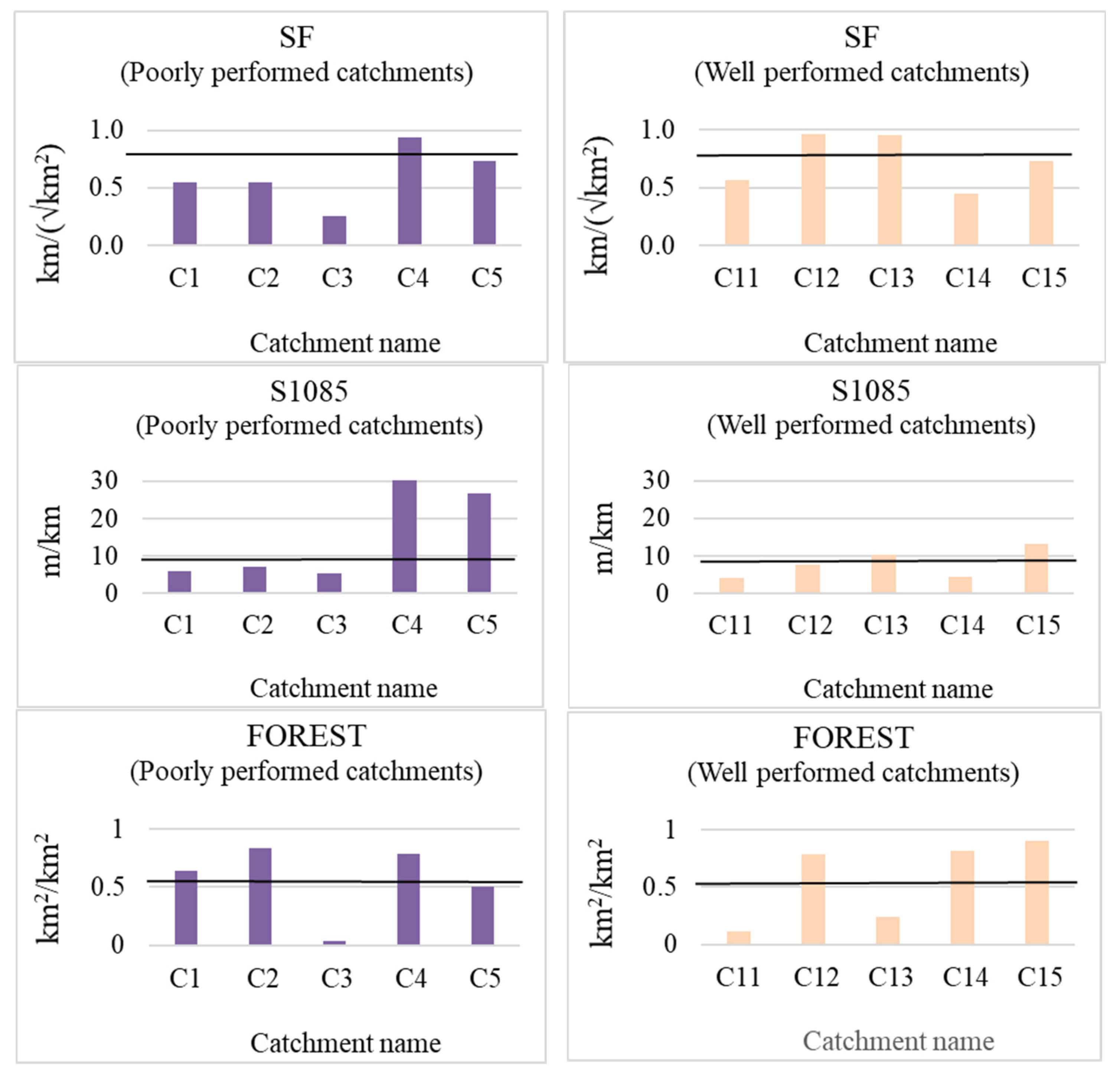
To evaluate the ANN model performance in depth for this study, five poorly performed catchments based on Qr values higher than 1.5 and five well-performed catchments based on Qr values in the range of 0.99–1.01 were selected. From Figure 8, it can be stated that the poorly performed catchments have relatively higher AREA and smaller SDEN values, and the well-performed catchments have a smaller AREA and a higher I62 and MAR (i.e., smaller and wetter catchments).

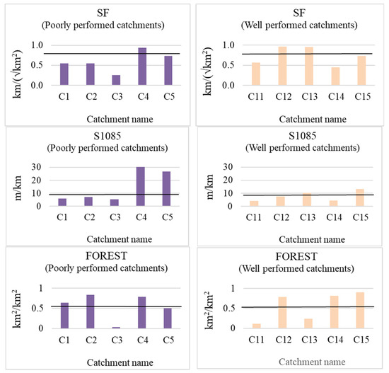
Figure 8.
Poorly performed catchments (C1, C2, C3, C4, and C5) and well-performed catchments (C11, C12, C13, C14, and C15) characteristics in the ANN (thick line represents the median value of a catchment characteristic considering all the 88 catchments).
5. Discussion
To compare the performance of the ANN model of this study, REr values for the six AEPs were compared with few other RFFA studies (Table 4). Rima et al. [51] compared the GAM and the parameter regression technique (PRT) for RFFA using data from NSW. In their study, the GAM outperformed the PRT with REr values ranging from 33 to 39%. In another study, Ali and Rahman [52] carried out a kriging-based RFFA study where REr values for NSW were found in the range of 28.2–35.9%. In another study, Zalnezhad et al. [43] compared SVM- and ANN-based RFFA models for Australia where the ANN model showed better performance than the SVM with REr values ranging from 33 to 54%. Similarly, Aziz et al. [41] compared ANN and GEP models with the QRT for southeast Australia. They revealed that the ANN outperformed the other models with REr values in the range of 36–46%. The ARR-recommended RFFA model [42] in Australia showed REr values ranging from 57.3 to 64.1% in NSW. The ARR-recommended RFFA model used a LOO validation technique and 558 catchments from eastern Australia. Compared to the other studies mentioned in Table 4, the ANN model of this study showed generally better/comparable results by showing lower REr values ranging from 31.9 to 39.6% in NSW.
Table 4.
Comparison of results of this study with other ones based on the literature.
Different methods perform differently; for example, the kriging method performs well in the dense stream gauging network. The eastern part of Australia is an ideal region for kriging-based methods, as this region has a dense stream gauging network. It should be noted that the ARR method used a larger dataset from all the Australian states and the LOO validation technique, whereas this study used a smaller dataset from the NSW state and adopted a split-sample validation technique. Generally, the LOO validation technique provides higher relative error values than the split-sample validation technique. The main limitations of the current study are that it compares only two RFFA methods (ANN and QRT) and it applies the ordinary least-squares method to develop the QRT method.
6. Conclusions
This study focuses on the development of RFFA for NSW, Australia, using data from 88 catchments. It compared QRT- and ANN-based RFFA models. A split-sample validation technique (70% data for training and 30% data for testing) was used to evaluate the performances of these models based on five statistical measures for six different AEPs. It was found that the ANN model outperforms the QRT model in particular for smaller return periods (Q2, Q5, and Q10); however, the median relative error values for higher return periods are similar for both the methods. For the ANN model, the median relative error values range from 31.89 to 39.56%, and are 36.30–40.40% for the QRT model. The ANN model outperforms the currently recommended RFFA model in the Australian Rainfall and Runoff (ARR) guideline. The ANN model generally performs better than the QRT for smaller and wetter catchments. It should be noted that for fewer catchments, the ANN models perform poorly, showing a high estimation error. To improve the ANN model in subsequent research, these unusual catchments need to be investigated further. Future studies should apply bootstrapping and Monte Carlo cross-validation to evaluate the model performance of the ANN model in a more comprehensive manner. The ANN model developed here should be tested in other Australian states so that it can be applied nationally.
Author Contributions
Data analysis, investigation, and manuscript drafting: N.A.; investigation and editing: R.S.M.H.R.; conceptualisation, investigation, editing, and supervision: K.H.; conceptualisation, editing, and supervision: A.R. All authors have read and agreed to the published version of the manuscript.
Funding
This research received no external funding.
Data Availability Statement
The data used in this study can be obtained from Australian Government authorities by paying a prescribed fee.
Acknowledgments
The authors would like to acknowledge the Australian Rainfall and Runoff Revision Project 5 team for providing some of the data used in this study. TUFLOW FLIKE was provided freely by the FLIKE sales team. Streamflow data were obtained from WaterNSW.
Conflicts of Interest
The authors declare no conflicts of interest.
References
- Jongman, B.; Ward, P.J.; Aerts, J.C.J.H. Global exposure to river and coastal flooding: Long term trends and changes. Glob. Environ. Change 2012, 22, 823–835. [Google Scholar] [CrossRef]
- Pinos, J.; Quesada-Román, A. Flood Risk-Related Research Trends in Latin America and the Caribbean. Water 2021, 14, 10. [Google Scholar] [CrossRef]
- Nofal, O.M.; Van De Lindt, J.W. Understanding flood risk in the context of community resilience modeling for the built environment: Research needs and trends. Sustain. Resilient Infrastruct. 2022, 7, 171–187. [Google Scholar] [CrossRef]
- Kuczera, G.; Franks, S. At-site flood frequency analysis. In Australian Rainfall & Runoff, Chapter 2, Book 3; Ball, J., Babister, M., Nathan, R., Weeks, W., Weinmann, E., Retallick, M., Testoni, I., Eds.; Commonwealth of Australia: Sydney, Australia, 2019. [Google Scholar]
- Cunnane, C. Review of statistical models for flood frequency estimation. In Hydrologic Frequency Modelling; Springer: Dordrecht, The Netherlands, 1987; pp. 49–95. [Google Scholar]
- Shu, C.; Ouarda, T.B.M.J. Flood frequency analysis at ungauged sites using artificial neural networks in canonical correlation analysis physiographic space. Water Resour. Res. 2007, 43. [Google Scholar] [CrossRef]
- Sen, Z. Regional drought and flood frequency analysis: Theoretical consideration. J. Hydrol. 1980, 46, 265–279. [Google Scholar] [CrossRef]
- Pilgrim, D.H.; Cordery, I. Chapter 9: Flood Runoff. Handbook of Hydrology; McGraw-Hill: New York, NY, USA, 1993. [Google Scholar]
- Rahman, A.; Haddad, K.; Zaman, M.; Kuczera, G.; E Weinmann, P. Design Flood Estimation in Ungauged Catchments: A Comparison Between the Probabilistic Rational Method and Quantile Regression Technique for NSW. Australas. J. Water Resour. 2011, 14, 127–139. [Google Scholar] [CrossRef]
- Dalrymple, T. Flood-Frequency Analyses (No. 1543); US Government Printing Office: Washington, DC, USA, 1960. [Google Scholar]
- Smith, A.; Sampson, C.; Bates, P. Regional flood frequency analysis at the global scale. Water Resour. Res. 2015, 51, 539–553. [Google Scholar] [CrossRef]
- Stedinger, J.R.; Tasker, G.D. Regional Hydrologic Analysis: 1. Ordinary, Weighted, and Generalized Least Squares Compared. Water Resour. Res. 1985, 21, 1421–1432. [Google Scholar] [CrossRef]
- Ouarda, T.B.M.J.; Ba, K.M.; Diaz-Delgado, C.; Carsteanu, A.; Chokmani, K.; Gingras, H.; Quentin, E.; Trujillo, E.; Bobée, B. Intercomparison of regional flood frequency estimation methods at ungauged sites for a Mexican case study. J. Hydrol. 2008, 348, 40–58. [Google Scholar] [CrossRef]
- Archfield, S.A.; Pugliese, A.; Castellarin, A.; Skøien, J.O.; Kiang, J.E. Topological and canonical kriging for design flood prediction in ungauged catchments: An improvement over a traditional regional regression approach? Hydrol. Earth Syst. Sci. 2013, 17, 1575–1588. [Google Scholar] [CrossRef]
- Faulkner, D.; Warren, S.; Burn, D. Design floods for all of Canada. Canad. Water Resour. J. Rev. Canad. Ressour. Hydr. 2016, 41, 398–411. [Google Scholar] [CrossRef]
- Chebana, F.; Charron, C.; Ouarda, T.B.M.J.; Martel, B. Regional Frequency Analysis at Ungauged Sites with the Generalized Additive Model. J. Hydrometeorol. 2014, 15, 2418–2428. [Google Scholar] [CrossRef]
- Msilini, A.; Charron, C.; Ouarda, T.B.M.J.; Masselot, P. Flood frequency analysis at ungauged catchments with the GAM and MARS approaches in the Montreal region, Canada. Can. Water Resour. J Rev. Can. Ressour. Hydr. 2022, 47, 111–121. [Google Scholar] [CrossRef]
- Kuichling, E. The Relation Between the Rainfall and the Discharge of Sewers in Populous Districts. Trans. Am. Soc. Civ. Eng. 1889, 20, 1–56. [Google Scholar] [CrossRef]
- Pilgrim, E.; Institution of Engineers Australia Pilgrim, D.H.; Canterford, R.P. Australian Rainfall and Runoff; Institution of Engineers: Sydney, Australia, 1987. [Google Scholar]
- Hosking, J.R.M.; Wallis, J.R. Some statistics useful in regional frequency analysis. Water Resour. Res. 1993, 29, 271–281. [Google Scholar] [CrossRef]
- Bates, B.C.; Rahman, A.; Mein, R.G.; Weinmann, P.E. Climatic and physical factors that influence the homogeneity of regional floods in southeastern Australia. Water Resour. Res. 1998, 34, 3369–3381. [Google Scholar] [CrossRef]
- Haddad, K.; Rahman, A. Regional flood frequency analysis in eastern Australia: Bayesian GLS regression-based methods within fixed region and ROI framework–Quantile Regression vs. Parameter Regression Technique. J. Hydrol. 2012, 430, 142–161. [Google Scholar] [CrossRef]
- Gupta, V.K.; Mesa, O.J.; Dawdy, D.R. Multiscaling theory of flood peaks: Regional quantile analysis. Water Resour. Res. 1994, 30, 3405–3421. [Google Scholar] [CrossRef]
- Rahman, A.S.; Khan, Z.; Rahman, A. Application of independent component analysis in regional flood frequency analysis: Comparison between quantile regression and parameter regression techniques. J. Hydrol. 2020, 581, 124372. [Google Scholar] [CrossRef]
- Sivakumar, B.; Singh, V.P. Hydrologic system complexity and nonlinear dynamic concepts for a catchment classification framework. Hydrol. Earth Syst. Sci. 2012, 16, 4119–4131. [Google Scholar] [CrossRef]
- Sharafati, A.; Haghbin, M.; Motta, D.; Yaseen, Z.M. The application of soft computing models and empirical formulations for hydraulic structure scouring depth simulation: A comprehensive review, assessment and possible future research direction. Arch. Comput. Methods Eng. 2021, 28, 423–447. [Google Scholar] [CrossRef]
- Jingyi, Z.; Hall, M. Regional flood frequency analysis for the Gan-Ming River basin in China. J. Hydrol. 2004, 296, 98–117. [Google Scholar] [CrossRef]
- Dawson, C.; Abrahart, R.; Shamseldin, A.; Wilby, R. Flood estimation at ungauged sites using artificial neural networks. J. Hydrol. 2006, 319, 391–409. [Google Scholar] [CrossRef]
- Allahbakhshian-Farsani, P.; Vafakhah, M.; Khosravi-Farsani, H.; Hertig, E. Regional flood frequency analysis through some machine learning models in semi-arid regions. Water Resour. Manag. 2020, 34, 2887–2909. [Google Scholar] [CrossRef]
- Vafakhah, M.; Bozchaloei, S.K. Regional analysis of flow duration curves through support vector regression. Water Resour. Manag. 2020, 34, 283–294. [Google Scholar] [CrossRef]
- Seckin, N.; Guven, A. Estimation of peak flood discharges at ungauged sites across Turkey. Water Resour. Manag. 2012, 26, 2569–2581. [Google Scholar] [CrossRef]
- Zorn, C.R.; Shamseldin, A.Y. Peak flood estimation using gene expression programming. J. Hydrol. 2015, 531, 1122–1128. [Google Scholar] [CrossRef]
- Garmdareh, E.S.; Vafakhah, M.; Eslamian, S.S. Regional flood frequency analysis using support vector regression in arid and semi-arid regions of Iran. Hydrol. Sci. J. 2018, 63, 426–440. [Google Scholar] [CrossRef]
- Bozchaloei, S.K.; Vafakhah, M. Regional analysis of flow duration curves using adaptive neuro-fuzzy inference system. J. Hydrol. Eng. 2015, 20, 06015008. [Google Scholar] [CrossRef]
- Desai, S.; Ouarda, T.B. Regional hydrological frequency analysis at ungauged sites with random forest regression. J. Hydrol. 2021, 594, 125861. [Google Scholar] [CrossRef]
- Esmaeili-Gisavandani, H.; Zarei, H.; Tehrani, M.R.F. Regional flood frequency analysis using data-driven models (M5, random forest, and ANFIS) and a multivariate regression method in ungauged catchments. Appl. Water Sci. 2023, 13, 139. [Google Scholar] [CrossRef]
- Tramblay, Y.; El Khalki, E.M.; Khedimallah, A.; Sadaoui, M.; Benaabidate, L.; Boulmaiz, T.; Boutaghane, H.; Dakhlaoui, H.; Hanich, L.; Ludwig, W.; et al. Regional flood frequency analysis in North Africa. J. Hydrol. 2024, 630, 130678. [Google Scholar] [CrossRef]
- Jarajapu, D.C.; Rathinasamy, M.; Agarwal, A.; Bronstert, A. Design flood estimation using extreme Gradient Boosting-based on Bayesian optimization. J. Hydrol. 2022, 613, 128341. [Google Scholar] [CrossRef]
- Mangukiya, N.K.; Sharma, A. Alternate pathway for regional flood frequency analysis in data-sparse region. J. Hydrol. 2024, 629, 130635. [Google Scholar] [CrossRef]
- Filipova, V.; Hammond, A.; Leedal, D.; Lamb, R. Prediction of flood quantiles at ungauged catchments for the contiguous USA using Artificial Neural Networks. Hydrol. Res. 2022, 53, 107–123. [Google Scholar] [CrossRef]
- Aziz, K.; Haque, M.M.; Rahman, A.; Shamseldin, A.Y.; Shoaib, M. Flood estimation in ungauged catchments: Application of artificial intelligence based methods for Eastern Australia. Stoch. Environ. Res. Risk Assess. 2017, 31, 1499–1514. [Google Scholar] [CrossRef]
- Rahman, A.; Haddad, K.; Kuczera, G.; Weinmann, E. Regional Flood Methods. In Australian Rainfall and Runoff: A Guide to Flood Estimation. Book 3, Peak Flow Estimation; Commonwealth of Australia: Sydney, Australia, 2019; pp. 105–146. [Google Scholar]
- Zalnezhad, A.; Rahman, A.; Nasiri, N.; Vafakhah, M.; Samali, B.; Ahamed, F. Comparing Performance of ANN and SVM Methods for Regional Flood Frequency Analysis in South-East Australia. Water 2022, 14, 3323. [Google Scholar] [CrossRef]
- Haddad, K.; Rahman, A.; Zaman, M.; Shrestha, S. Applicability of Monte Carlo cross validation technique for model development and validation using generalised least squares regression. J. Hydrol. 2013, 482, 119–128. [Google Scholar] [CrossRef]
- Mcculloch, W.S.; Pitts, W.H. A logical calculus of the ideas immanent in nervous activity. Bull. Math. Biophys. 1943, 5, 115–133. [Google Scholar] [CrossRef]
- Rumelhart, D.E.; Hinton, G.E.; Williams, R.J. Learning representations by back-propagating errors. Nature 1986, 323, 533–536. [Google Scholar] [CrossRef]
- Rathore, P.S.; Dadich, N.; Jha, A.; Pradhan, D. Effect of learning rate on neural network and convolutional neural network. Int. J. Eng. Res. Technol. 2018, 6, 1–8. [Google Scholar]
- Ying, X. An overview of overfitting and its solutions. In Journal of Physics: Conference Series; IOP Publishing: Bristol, UK, 2019; Volume 1168, p. 022022. [Google Scholar]
- Deng, T. Effect of the number of hidden layer neurons on the accuracy of the back propagation neural network. Highlights Sci. Eng. Technol. 2023, 74, 462–468. [Google Scholar] [CrossRef]
- Jackson, E.K.; Roberts, W.; Nelsen, B.; Williams, G.P.; Nelson, E.J.; Ames, D.P. Introductory overview: Error metrics for hydrologic modelling—A review of common practices and an open source library to facilitate use and adoption. Environ. Model. Softw. 2019, 119, 32–48. [Google Scholar] [CrossRef]
- Rima, L.; Haddad, K.; Rahman, A. Generalised Additive Model-Based Regional Flood Frequency Analysis: Parameter Regression Technique Using Generalised Extreme Value Distribution. Water 2025, 17, 206. [Google Scholar] [CrossRef]
- Ali, S.; Rahman, A. Development of a kriging-based regional flood frequency analysis technique for South-East Australia. Nat. Hazards 2022, 114, 2739–2765. [Google Scholar] [CrossRef]
Disclaimer/Publisher’s Note: The statements, opinions and data contained in all publications are solely those of the individual author(s) and contributor(s) and not of MDPI and/or the editor(s). MDPI and/or the editor(s) disclaim responsibility for any injury to people or property resulting from any ideas, methods, instructions or products referred to in the content. |
© 2025 by the authors. Licensee MDPI, Basel, Switzerland. This article is an open access article distributed under the terms and conditions of the Creative Commons Attribution (CC BY) license (https://creativecommons.org/licenses/by/4.0/).