Optimizing Hydrodynamic Regulation in Coastal Plain River Networks in Eastern China: A MIKE11-Based Partitioned Water Allocation Framework for Flood Control and Water Quality Enhancement

Abstract

The effective management of river networks in coastal plains is crucial to flood control, water quality improvement, and sustainable flow distribution. This study aims to optimize the hydrodynamic performance of a plain river network in eastern China through water diversion and circulation scheduling, addressing challenges such as channel narrowing and sedimentation. This research study utilized a partitioned water allocation approach modeled in MIKE11 to simulate the effects of various diversion projects, including locks and connecting rivers, on the primary conveyance channel and supporting rivers. The simulation results indicated that flow velocities exceeded 0.1 m/s in most rivers, with significant improvements in flood discharge and water quality in the main conveyance channel and one supporting river. However, some sections of the network showed poor hydrodynamic performance due to narrow channels, encroachment, and sedimentation, and smaller rivers exhibited inadequate flow capacity. The findings provide critical insights for optimizing hydrodynamic regulation in coastal plain river systems, emphasizing the need to address specific issues to enhance overall network performance and flood resilience.

1. Introduction

The effective management of river networks is crucial to flood control, water quality improvement, and ecological restoration, particularly in coastal plain areas. As development accelerates, maintaining the hydrodynamic balance of these systems becomes increasingly complex. The concept of diversion loop capacity, which refers to the flow capacity of a river network influenced by water level changes, plays a significant role in the regulation of water resources and flood mitigation [1]. Optimizing hydraulic connectivity through efficient gate and dam regulation can enhance the overall performance of the diversion loop, offering social, economic, and ecological benefits. However, the complexity of river systems and the diverse factors affecting their hydrodynamics, such as sedimentation, encroachment, and flow direction, present significant challenges. The focus of this study is optimizing hydrodynamic performance in plain river networks through effective water allocation strategies that improve both flood conveyance and water quality.

The hydrodynamic modeling of rivers has evolved significantly since the late 18th century, with early research focusing on wave speed and flow dynamics. In 1775, Laplace and Lagrange introduced a formula for wave speed, marking the beginning of hydrodynamic research. Later, in 1843, St. Venant developed the basic equations of motion for viscous incompressible fluids, which laid the foundation for subsequent river modeling. The St. Venant equations, further refined in 1871, mathematically describe non-constant flow phenomena and have been widely used to model river dynamics in both theoretical and applied studies [2]. Over the years, these equations were solved numerically by discretizing time and space derivatives, with various methods such as finite difference, finite element, and finite volume approaches being employed to solve one-dimensional tidal flow equations [3]. Notable scholars like Droulers [4], Nguyen and Kawano [5], and Sen and Garg [6], have contributed to enhancing the accuracy of these numerical methods, including the hierarchical and three-level solution techniques for solving one-dimensional St. Venant equations.

Two-dimensional models, which assume the uniform distribution of physical variables in the vertical direction, emerged in the 1950s to study water flow motion in simpler systems. These models are particularly useful for simulating water bodies like rivers, lakes, and coastal regions, where stratification effects can often be neglected. DeViend [7] performed extensive experiments on hydrodynamic factors affecting river channels, particularly in curved flumes, which provided valuable data for improving two-dimensional modeling techniques. River networks, however, are inherently three-dimensional systems where flow direction, water depth, and topography vary. The complexity of these systems, especially in natural river channels, has led to the development of three-dimensional hydrodynamic models. Lin [8] and Wu [9] contributed to the hydrodynamic modeling of open channels by addressing three-dimensional problems, and Jiang et al. [10] used the finite volume method to model material transport in rivers. Chen et al. [11] applied three-dimensional hydrodynamic models to study sediment and phosphorus dynamics in Lake Okeechobee, USA, shedding light on the interaction between hydrodynamics and water quality.

Alongside advances in hydrodynamic modeling, significant research has focused on optimizing water diversion and flow regulation systems. Nie et al. [12] developed a mathematical model using a genetic algorithm to construct an emergency scheduling system for a long-distance aqueduct, and its operation was analyzed. Zhao et al. [13] focused on the sluice gate scheduling system in an irrigation area, proposing a joint scheduling framework for a distributed sluice gate community. To improve the characterization of water quality and algal transport in trunk canals under complex scheduling conditions, Jing et al. [14] employed principal component analysis (PCA) to study the key factors affecting algae, creating a comprehensive index to reflect the distribution of water quality and algae transport in the MR trunk canal. This allowed for the exploration of how environmental and hydrodynamic factors change within the river–gate coupling system. Zhang et al. [15] combined water quantity and quality dispatch models by using a Backpropagation algorithm and soil and water evaluation tools to explore the efficient operation of dams and locks at the basin scale. Yu et al. [16,17] conducted simulations to address the ecological management of river networks, specifically focusing on sluice gate operations, flood management, and ecological dispatching in plain areas, while studying “one-tide” flooding, drainage, and ecological dispatching issues. Zhang et al. developed a numerical model for a single river reach as a human-made case study, analyzing its downstream regulation capabilities. Similarly, Weng et al. [18] proposed a multi-gate management model based on ecological principles, utilizing the MIKE21 model and the Physical Habitat Simulation (PHABSIM) model to calculate flow dynamics, incorporating parameters such as velocity, water depth, and salinity.

Water diversion circulation routes are optimized based on a range of evaluation indicators selected from different perspectives. These indicators focus on water system patterns, structural connectivity, and hydraulic connectivity. While much attention has been given to water system patterns and structural connectivity, hydraulic connectivity has often been less emphasized. Cui et al. [19] analyzed the diversion circulation of two river networks under high- and low-flow conditions, comparing them with structural connectivity using graph theory. Brierley et al. [20], Tetzlat et al. [21], and Ali et al. [22] similarly examined the structural connectivity of river networks in relation to diversion circulation. Jain et al. [23] categorized diversion circulation into active, inactive, partially active, and non-connected states based on water system patterns and structural connectivity and developed the Ganges River health evaluation system. Phillips et al. [24] established a framework for evaluating hydraulic connectivity in rivers, considering factors like flow resistance and hydrological processes.

Inter-basin hydrodynamic regulation not only improves the distribution of water resources but also accelerates the hydrodynamic processes in receiving river networks, restoring the ecological health of these systems, slowing wetland degradation, and enhancing water body environments. Various international projects have been initiated to improve basin hydrodynamics and restore river network environments, such as the northern Lake Teganuma water regulation project in Chiba Prefecture, Japan; the Lake Pontchartrain diversion project in Louisiana, USA; the Ruhr River water transfer project in Germany; and the Moscow River water regulation project in Russia [25,26,27]. These projects illustrate the global efforts to optimize water resource management and restore river ecosystems through hydrodynamic regulation.

While previous research has primarily focused on individual aspects of river system management, there is a need for integrated approaches that consider both hydrodynamics and the ecological impacts of water diversion in plain river networks. This study aims to optimize the hydrodynamic performance of a plain river network in eastern China through effective water allocation strategies, particularly by regulating gates and dams to improve flood conveyance and water quality. We employ a partitioned water allocation model in DHI MIKE11 [28] to simulate the hydrodynamic effects of water diversion in a river network influenced by various structural and operational factors. The focus of this study is to explore how water diversion and circulation scheduling can enhance hydraulic performance while addressing challenges such as channel narrowing, sedimentation, and flow capacity in smaller river sections. Our findings provide valuable insights into optimizing river network management strategies, ensuring that flood control and water quality objectives are met while maintaining the ecological balance of the system.

2. Materials and Methods

2.1. Modeling

The numerical simulation of river networks is based on the St. Venant equations for open-channel flow, with DHI MIKE11 [28] serving as the modeling platform. The main governing equations are as follows.

(1)

Open-Channel Flow Control Equations

The one-dimensional unsteady flow fundamental equations describing the motion of water in open channels are the St. Venant equations, which include the continuity equation and the momentum equation:

$$B_T{\displaystyle \frac{\partial Z}{\partial t}}+{\displaystyle \frac{\partial Q}{\partial x}}=q$$

(1)

$${\displaystyle \frac{\partial Q}{\partial t}}+{\displaystyle \frac{\partial }{\partial t}}\left({\displaystyle \frac{Q^2}{A}}\right)+gA{\displaystyle \frac{\partial Z}{\partial x}}+gA{\displaystyle \frac{\left|Q\right|Q}{K^2}}=0$$

(2)

$q$—lateral inflow into the river channel (m³/s);

$B_T$—equivalent river width (m);

$A$—cross-sectional area of flow (m²);

$Z$—water level at the section (m);

$Q$—discharge at the section (m³/s);

$K$—discharge modulus (m³/s).

(2)

Node Equations

River segments are interconnected, and the points of connection are known as nodes. Each node must satisfy two continuity conditions: the flow continuity condition and the dynamic continuity condition.

① Flow Continuity Condition

The flow at each node must adhere to the principle of mass conservation, meaning that the flow entering the node at any given moment must equal the change in the node’s water storage:

$${\displaystyle \sum }_{j=1}^n{Q}_i^j={\displaystyle \frac{d{\omega }_i}{dt}}$$

(3)

$Q_i^j$—flow discharge of river j entering node i (m³/s);

${\omega }_i$—volume of water stored at node I (m³);

$n$—number of rivers flowing into node i.

Nodes may have regulation and storage function, and their continuity equation takes the following form:

$${\displaystyle \frac{\partial H}{\partial t}}={\displaystyle \frac{\sum Q_t}{S_t}}$$

(4)

$S_t$—cross-sectional area of flow at the node at time t (m²);

$H$—water level at the node (m);

$\sum Q_t$—sum of node flows at time t (m³/s).

The differential form of the node equation is

$$H_{t+\Delta t}=H_t+{\displaystyle \frac{\sum {\overline{Q}}_t\Delta t}{{\overline{S}}_t}}$$

(5)

For nodes without storage capacity,

$$\sum {\overline{Q}}_t=0$$

(6)

② Dynamic Connection Conditions

At a certain node, the water level and flow velocity at each connected river cross-section must comply with the actual dynamic connection conditions, which must satisfy the Bernoulli equation.

If the node has no storage effect, then the dynamic connection conditions are simplified to

$$H_i=H_n$$

(7)

$H_i$—water level of the river section connected to the node (m);

$H_n$—water level at the node (m).

If a gate, weir, or significant change occurs in the cross-sectional area at the node, the dynamic connection condition is

$$a{H}_i+b{Q}_i+c{H}_j+d{Q}_j=e$$

(8)

When the node is a gate or weir, e is not zero; when the node shows a significant change in cross-sectional area, e is zero.

The entire river network is a system composed of multiple river sections and connecting nodes. The governing equation for the water volume within the river network’s water volume is derived by combining the governing equations for each river section with the connection conditions at each node, as well as the initial and boundary conditions. By numerically solving this system of differential equations, hydraulic variables such as water level and flow velocity at specified cross-sections along the river at each node can be determined.

(3)

Internal Boundary Treatment

The model accounts for three primary types of internal boundary conditions: concentrated lateral inflow, sudden changes in cross-sectional flow area, and flow over weirs and gates.

① Concentrated Lateral Inflow: For concentrated lateral inflow, a virtual river segment with Δx_j = 0 can be assumed to satisfy the basic continuity equation

$$\left\{\begin{array}{c}{Z}_j=Z_{j+1}\\ Q_j+Q_f=Q_{j+1}\end{array}\right.$$

(9)

$Z_j$, $Z_{j+1}$—water levels at sections j and j+1 (m);

$Q_j$, $Q_{j+1}$—flow velocity at sections j and j+1 (m³/s);

$Q_f$—concentrated lateral inflow (m³/s).

② Sudden Changes in Flow Cross-Section: After generalizing the boundary as a series of one-dimensional river segments connected end to end, the cross-sectional areas at each section may not change continuously, and sudden changes in the flow cross-section may occur. The compatibility condition for this situation is

$$\left\{\begin{array}{c}{Q}_j=Q_{j+1}\\ Z_j+{\displaystyle \frac{u_j^2}{2g}}=Z_{j+1}+{\displaystyle \frac{u_{j+1}^2}{2g}}+\zeta {\displaystyle \frac{{\left(u_j-u_{j+1}\right)}^2}{2g}}\end{array}\right.$$

(10)

$u_j$,$u_{j+1}$—flow velocities at sections j and j+1 (m/s);

$\zeta$—local resistance coefficient;

$g$—acceleration due to gravity (m²/s).

③ Flow Over Weirs and Gates: In practical engineering, gates are commonly installed in rivers to control the water volume or water level. There are three scenarios for the flow of water through these gates:

(1)

Close the gate

$$Q=0$$

(11)

(2)

Open-gate diversion ($Z_d>Z_u$)

If $\left(Z_u-Z_0\right)\le {\displaystyle \frac{2}{3}}\left(Z_d-Z_0\right)$, for free outflow,

$$Q=u_1\varphi B\sqrt{2g}{\left(Z_d-Z_0\right)}^{{\displaystyle \frac{3}{2}}}$$

(12)

If $\left(Z_u-Z_0\right)>{\displaystyle \frac{2}{3}}\left(Z_d-Z_0\right)$, for flooding out of the stream,

$$Q=u_2\varphi B\sqrt{2g}\left(Z_d-Z_0\right)\sqrt{Z_d-Z_u}$$

(13)

(3)

Open-gate drainage ($Z_d<Z_u$)

If $\left(Z_d-Z_0\right)\le {\displaystyle \frac{2}{3}}\left(Z_u-Z_0\right)$, for free outflow,

$$Q=u_1\varphi B\sqrt{2g}{\left(Z_u-Z_0\right)}^{{\displaystyle \frac{3}{2}}}$$

(14)

If $\left(Z_d-Z_0\right)>{\displaystyle \frac{2}{3}}\left(Z_u-Z_0\right)$, for flooding out of the stream,

$$Q=u_2\varphi B\sqrt{2g}\left(Z_u-Z_0\right)\sqrt{Z_u-Z_d}$$

(15)

$u_1$—flow coefficient of free outflow;

$u_2$—flow coefficient of the submerged outflow;

$\varphi$—relative opening height of the gate;

$B$—width of the gate hole (m);

$Q$—drainage flow discharge (m³/s);

$Z_u$—water level upstream from the gate (m);

$Z_d$—water level downstream from the gate (m);

$Z_0$—gate bottom elevation (m).

Furthermore, the outflow from the pumping station is determined based on the designed pumping capacity and the dispatching mode.

2.2. Model Solving

The models were solved via MIKE11 [28] developed by the Danish Hydraulic Institute (DHI), a widely recognized and reliable tool for river hydraulic simulations. Mike11 is known for its strong capabilities in river hydraulics and water environment modeling, making it a trusted software application for the numerical simulation of river networks. The basic principle behind solving the model is starting from tributaries to main streams, from upstream to downstream. That is, the river network is decomposed into a sequence of individual rivers, each solved using the calculation method for single rivers.

The coastal river network within the defined calculation range was simplified and processed according to the relevant conventions of calculation software, as shown in Figure 1. The major rivers in the study area are listed in

Table 1. Major rivers in the study area.

	River Name	Abbreviation
1	Datang River	DT River
2	Husha River	HS River
3	Dongheng River	DH River
4	Chaotang River	CT River
5	Sizhaopu River	SP River
6	Daheng River	DA River
7	Liuzao River	LZ River
8	Wuzao River	WZ River
9	Sizao River	SZ River
10	Sanzao River	SA River
11	Zhoutang River	ZT River
12	Xianshenglu River	XS River
13	Shishan River	SS River
14	Dongcheng River	DC River
15	Jinshanhou River	JS River
16	Danshanmiao River	DS River
17	Yubo River	YB River
18	Maojiacao River	MJ River
19	Xiaoji River	XJ River
20	Dahekou River	DK River
21	Huatuodian River	HT River
22	Zhaojialu River	ZL River
23	Zhong River	ZH River
24	Zhoujia River	ZJ River
25	Laoyizao River	LY River
26	Xiyangsi River	XY River
27	Chengdongxincun River	CD River
28	Xinan River	XA River
29	Mingshanlu River	ML River
30	Miaoshan River	MS River
31	Xiwuzao River	XW River
32	Xisizao River	XZ River
33	Xiliuzao River	XL River
34	Xisanzao River	XI River
35	Fanghuanglu River	FH River
36	Jiangjiayan River	JY River
37	Lijiacao River	LJ River
38	Jibu River	JB River
39	Yao River	YA River

. Based on the 38 branches shown in Figure 1, the entire central area river network was divided into 51 calculation sections. In total, 315 calculation cross-sections were established across these 51 sections to meet the needs of the simulation. The roughness of the side walls for each section was preliminarily set between 0.025 and 0.035. For the calculation process, it was assumed that there is only one flow entrance on the west side of the Datang (DT) River and one drainage outlet on the Sanzao (SA) River extension. The drainage outlet is controlled by a gate that regulates the water level at the outlet, which ranges from 1.95 m to 0.9 m. Reasonable values were chosen for different calculation schemes, and the calculation time step was set to 60 s.

The model was calibrated using trial-and-error and sensitivity analyses, incorporating historical hydrological records. Key parameters (roughness, water level, and boundary conditions) were adjusted to ensure that the simulated hydrodynamics matched the regional hydrological regime, such as the annual flood peak in the main rivers.

The following section presents the different hydraulic characteristic simulation schemes designed for different calculation purposes. It also includes an analysis of the numerical simulation results for these schemes to estimate the hydraulic characteristics after the implementation of the central area river network water diversion loop project. These results offer valuable insights into the potential improvements to the river network’s water environment and provide the necessary technical data for the next phase of the project, formulating the water diversion loop project’s dispatch operation plan.

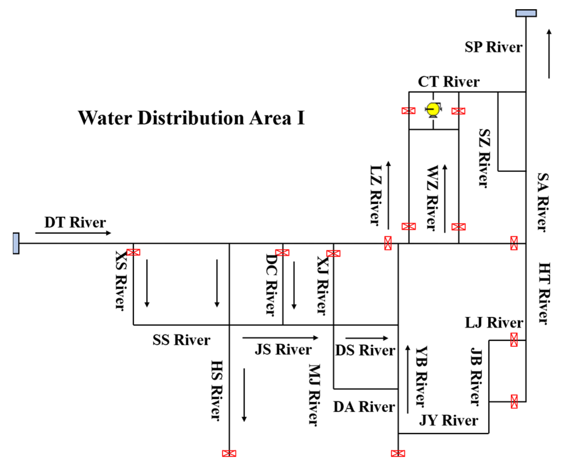
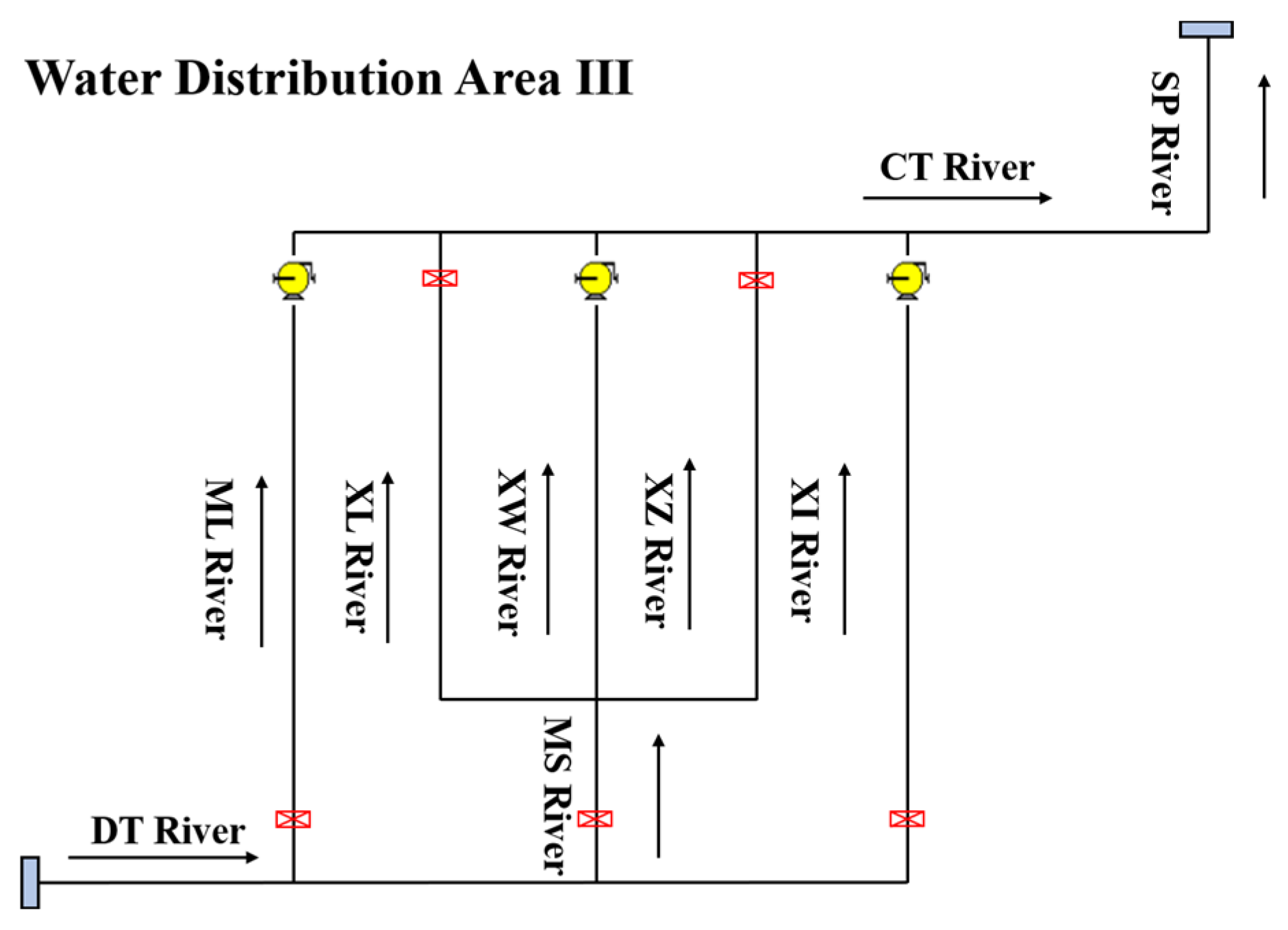
2.3. Design of Zoned Water Distribution Programs

According to the topographic features and river network characteristics of the study area, combined with the layout of control buildings at the river network nodes, a zoning water distribution scheme is designed to optimize the system’s response to low-flow conditions. The proposed zoned water distribution program divides the river network of the study area into three water distribution areas, labeled I to III, from east to west. Building on the general network (Figure 1), Figure 2, Figure 3 and Figure 4 illustrate detailed water distribution routes and control structures. Specifically, the design incorporates the implications of the diversion loop-through to address critical hydrodynamic challenges; these loop-throughs serve as interconnected flow paths in each zone, allowing controlled water redirection to bypass narrow or silted channels (as in Figure 4 for area III). The loop-throughs in Figure 4 enhance hydraulic connectivity, reduce low-flow stagnation, and boost flood discharge efficiency by creating alternative routes.

3. Results

3.1. Calculation Conditions

Based on the river network zoning results for the study area and the layout of the junction control buildings, a numerical simulation is conducted to evaluate the operational conditions of the high-flow zoned water distribution scheme.

Table 2. Main calculation conditions for zoned water distribution.

Water Distribution Area	Initial Water Level of River Network (m)	SP River Outlet Water Level (m)	Condition No.
I	1.75	0.9	1
		1.75	2
II	1.75	0.9	3
		1.75	4
III	1.75	0.9	5
		1.75	6

outlines conditions for evaluating high-flow scenarios, where SP River outlet levels regulate the hydraulic gradients in the network.

3.2. Simulation Results and Analysis

For the boundary and initial conditions of the water zone distribution scheme mentioned above, six scenarios (Cases 1–6, Table 2) were designed for calculation. A numerical simulation was then conducted using software. The key calculation results for these scenarios are summarized in

Table 3. Numerical simulation results for Case 1.

River	Flux (m3/s)	Inlet Level (m)	Outlet Level (m)	Maximum Flow Velocity (m/s)	Minimum Flow Velocity (m/s)	Flow
CT River 8	4.000	1.290	1.290	0.180	0.110	West → East
CT River 9	7.600	1.290	1.290	0.290	0.270
DT River 1	12.000	1.880	1.880	0.190	0.190	West → East
DT River 2	12.000	1.860	1.850	0.191	0.190
DT River 3	8.800	1.850	1.820	0.246	0.226
DT River 4	8.800	1.820	1.815	0.265	0.250
DT River 5	8.800	1.815	1.810	0.285	0.285
DT River 6	1.800	1.810	1.810	0.060	0.060
DT River 7	1.780	1.810	1.810	0.060	0.060
DT River 8	0.000	1.810	1.410	0.000	0.000
DT River 9	7.000	1.410	1.409	0.280	0.280
DT River 10	3.100	1.409	1.409	0.120	0.120
DT River 11	0.600	1.409	1.408	0.025	0.025
DA River 1	9.500	1.640	1.560	0.400	0.340	West → East
DA River 2	5.000	1.560	1.550	0.210	0.190
LZ River	3.900	1.409	1.290	0.320	0.150	South → North
WZ River	3.700	1.409	1.289	0.230	0.140	South → North
SZ River	0.150	1.330	1.290	0.026	0.004	South → North
SP River	12.000	1.290	0.900	0.800	0.600	South → North
SA River	4.200	1.408	1.290	0.320	0.170	South → North
ZT River	0.150	1.330	1.330	0.018	0.014	East → West
XS River	3.200	1.850	1.840	0.360	0.013	North → South
SS River	3.200	1.840	1.800	0.345	0.200	West → East
HS River 1	7.000	1.810	1.800	0.280	0.250	North → South
HS River 2	9.500	1.800	1.640	0.320	0.290
DC River	1.750	1.810	1.800	0.280	0.110	South → North
JS River 1	0.800	1.810	1.800	0.045	0.050	West → East
JS River 2	2.500	1.800	1.790	0.230	0.210	West → East
DS River	1.300	1.790	1.450	0.580	0.580	West → East
YB River 1	7.000	1.410	1.450	0.370	0.350	South → North
YB River 2	5.700	1.450	1.560	0.310	0.210	South → North
MJ River	1.300	1.790	1.790	0.065	0.065	South → North
XJ River	0.020	1.810	1.790	0.000	0.002	South → North
DK River	1.300	1.790	1.530	0.930	0.850	East → West
HT River	5.000	1.410	1.550	0.340	0.320	South → North

,

Table 4. Numerical simulation results for Case 2.

River	Flux (m3/s)	Inlet Level (m)	Outlet Level (m)	Maximum Flow Velocity (m/s)	Minimum Flow Velocity (m/s)	Flow
CT River 8	4.300	1.855	1.855	0.140	0.080	West → East
CT River 9	8.000	1.855	1.853	0.220	0.080
DT River 1	12.000	2.140	2.120	0.166	0.166
DT River 2	12.000	2.120	2.120	0.167	0.167
DT River 3	8.800	2.120	2.109	0.210	0.197
DT River 4	8.800	2.109	2.100	0.230	0.215
DT River 5	8.800	2.100	2.095	0.250	0.250
DT River 6	2.000	2.095	2.095	0.058	0.058
DT River 7	2.000	2.095	2.095	0.058	0.058
DT River 8	0.000	2.095	1.894	0.000	0.000
DT River 9	7.000	1.894	1.890	0.000	0.000
DT River 10	2.700	1.890	1.890	0.082	0.082
DT River 11	1.000	1.890	1.890	0.030	0.030
DA River 1	9.000	1.990	1.960	0.320	0.280	West → East
DA River 2	5.000	1.960	1.950	0.170	0.160
LZ River	4.300	1.890	1.855	0.210	0.113	South → North
WZ River	3.700	1.890	1.855	0.150	0.100	South → North
SZ River	0.125	1.865	1.853	0.017	0.004	South → North
SP River	12.000	1.853	1.750	0.430	0.430	South → North
SA River	3.900	1.890	1.853	0.210	0.120	South → North
ZTH River	0.130	1.867	1.867	0.010	0.009	East → West
XS River	3.200	2.120	2.110	0.300	0.114	North → South
SS River	3.200	2.110	2.090	0.290	0.170	West → East
HS River 1	6.800	2.090	2.090	0.235	0.210	North → South
HS River 2	9.000	2.090	1.995	0.270	0.250
DC River	1.800	2.095	2.090	0.220	0.090	South → North
JS River 1	0.800	2.090	2.090	0.040	0.040	West → East
JS River 2	2.500	2.090	2.080	0.200	0.200	West → East
DS River	1.300	2.080	1.908	0.470	0.470	West → East
YB River 1	7.000	1.893	1.908	0.280	0.260	South → North
YB River 2	5.500	1.908	1.955	0.240	0.160	South → North
MJ River	1.400	2.080	2.080	0.070	0.070	South → North
XJ River	0.000	2.095	2.080	0.000	0.000	South → North
DK River	1.500	2.080	1.940	0.800	0.700	East → West
HT River	5.000	1.950	1.890	0.260	0.200	South → North

,

Table 5. Numerical simulation results for Case 3.

River	Flux (m3/s)	Inlet Level (m)	Outlet Level (m)	Maximum Flow Velocity (m/s)	Minimum Flow Velocity (m/s)	Flow
CT River 5	6.500	1.918	1.910	0.188	0.180	West → East
CT River 6	10.000	1.910	1.899	0.270	0.191
CT River 7	12.000	1.899	1.872	0.380	0.350
CT River 8	12.000	1.872	1.866	0.400	0.244
CT River 9	12.000	1.866	1.853	0.340	0.320
DT River 1	12.000	2.010	1.995	0.177	0.177	West → East
DT River 2	12.000	1.995	1.995	0.178	0.178
DT River 3	12.000	1.995	1.955	0.300	0.300
DT River 4	12.000	1.955	1.934	0.340	0.320
DT River 5	5.500	1.934	1.932	0.168	0.168
DT River 6	5.500	1.932	1.928	0.169	0.169
DT River 7	0.300	1.928	1.928	0.010	0.010
DT River 8	0.300	1.928	1.928	0.010	0.010
DT River 9	0.000	1.928	1.928	0.000	0.000
ZL River	6.500	1.934	1.918	0.160	0.130	South → North
ZH River	1.750	1.921	1.917	0.065	0.055	South → North
ZJ River 1	5.200	1.928	1.921	0.160	0.210	South → North
ZJ River 2	3.300	1.921	1.919	0.095	0.095
ZJ River 3	1.800	1.919	1.917	0.050	0.048
ZJ River 4	3.600	1.917	1.910	0.130	0.100
LYA River	0.280	1.928	1.928	0.030	0.010	South → North
XY River	1.550	1.919	1.909	0.150	0.150	West → East
CD River	0.087	1.928	1.920	0.100	0.009	West → East
XA River 1	0.380	1.909	1.909	0.190	0.013	South → North
XA River 2	1.900	1.909	1.899	0.090	0.074	South → North
SP River	12.000	1.853	1.750	0.440	0.430	South → North

,

Table 6. Numerical simulation results for Case 4.

River	Flux (m3/s)	Inlet Level (m)	Outlet Level (m)	Maximum Flow Velocity (m/s)	Minimum Flow Velocity (m/s)	Flow
CT River 5	6.940	1.435	1.418	0.255	0.247	West → East
CT River 6	10.200	1.418	1.395	0.360	0.350
CT River 7	12.000	1.395	1.330	0.490	0.450
CT River 8	12.000	1.330	1.315	0.530	0.320
CT River 9	12.000	1.315	1.285	0.450	0.320
DT River 1	12.000	1.640	1.610	0.216	0.216	West → East
DT River 2	12.000	1.610	1.600	0.220	0.220
DT River 3	12.000	1.600	1.520	0.390	0.370
DT River 4	12.000	1.520	1.470	0.430	0.420
DT River 5	5.050	1.470	1.470	0.204	0.204
DT River 6	5.050	1.470	1.460	0.204	0.204
DT River 7	0.200	1.460	1.460	0.206	0.206
DT River 8	0.200	1.460	1.460	0.010	0.010
DT River 9	0.000	1.460	1.460	0.010	0.010
ZL River	7.000	1.470	1.435	0.220	0.175	South → North
ZH River	1.600	1.440	1.435	0.085	0.070	South → North
ZJ River1	4.800	1.460	1.440	0.280	0.200	South → North
ZJ River 2	3.100	1.440	1.440	0.115	0.110
ZJ River 3	1.700	1.440	1.430	0.066	0.064
ZJ River 4	3.400	1.430	1.417	0.160	0.130
LYA River	0.260	1.460	1.460	0.042	0.011	South → North
XY River	1.350	1.440	1.420	0.175	0.066	West → East
CD River	0.076	1.440	1.460	0.011	0.011	West → East
XA River 1	0.340	1.420	1.420	0.230	0.015	South → North
XA River 2	1.700	1.420	1.395	0.120	0.100	South → North
SP River	12.000	1.285	0.900	0.800	0.606	South → North

,

Table 7. Numerical simulation results for Case 5.

River	Flux (m3/s)	Inlet Level (m)	Outlet Level (m)	Maximum Flow Velocity (m/s)	Minimum Flow Velocity (m/s)	Flow
CT River 1	3.400	1.958	1.955	0.104	0.084	West → East
CT River 2	6.400	1.955	1.954	0.180	0.170
CT River 3	8.400	1.954	1.956	0.230	0.220
CT River 4	12.000	1.956	1.940	0.330	0.330
CT River 5	12.000	1.940	1.915	0.340	0.330
CT River 6	12.000	1.915	1.900	0.330	0.350
CT River 7	12.000	1.900	1.875	0.380	0.350
CT River 8	12.000	1.875	1.866	0.400	0.245
CT River 9	12.000	1.866	1.854	0.340	0.320
DT River 1	12.000	2.015	1.995	0.176	0.176
DT River 2	8.600	1.995	1.995	0.126	0.126
DT River 3	3.600	1.995	1.990	0.085	0.009
ML River	3.400	1.995	1.955	0.150	0.112	South → North
MS River	4.900	1.995	1.960	0.280	0.180
XW River	2.900	1.960	1.955	0.088	0.086
XL River	0.000	1.960	1.955	0.000	0.000
XZ River	2.000	1.960	1.954	0.090	0.076
XI River	3.600	1.990	1.950	0.190	0.085
SP River	12.000	1.853	1.750	0.430	0.350

and

Table 8. Numerical simulation results for Case 6.

River	Flux (m3/s)	Inlet Level (m)	Outlet Level( m)	Maximum Flow Velocity (m/s)	Minimum Flow Velocity (m/s)	Flow
CT River 1	2.100	1.250	1.250	0.092	0.072	West → East
CT River 2	4.100	1.250	1.250	0.170	0.072
CT River 3	5.500	1.250	1.250	0.215	0.205
CT River 4	8.000	1.250	1.235	0.320	0.310
CT River 5	8.000	1.235	1.200	0.330	0.320
CT River 6	8.000	1.200	1.180	0.320	0.310
CT River 7	8.000	1.180	1.140	0.380	0.340
CT River 8	8.000	1.140	1.130	0.400	0.235
CT River 9	8.000	1.130	1.110	0.330	0.310
DT River 1	8.000	1.370	1.340	0.173	0.173
DT River 2	5.900	1.340	1.340	0.132	0.130
DT River 3	2.500	1.340	1.330	0.090	0.100
ML River	2.100	1.340	1.250	0.160	0.106	South → North
MS River	3.400	1.340	1.270	0.300	0.195
XW River	2.150	1.270	1.250	0.106	0.094
XL River	0.000	1.270	1.260	0.000	0.000
XZ River	1.350	1.270	1.250	0.104	0.080
XI River	2.500	1.330	1.250	0.220	0.080
SP River	8.000	1.110	0.900	0.455	0.530

, providing a detailed overview of the simulation outcomes under various conditions.

When the diversion loop-through flow is set to 12 m³/s, the hydraulic simulation results for the water distribution scheme of each sub-district show significant improvements in the flow conditions across the river network. The main findings from the analysis of these results are as follows:

(1)

The flow velocities in each section of the river network are conducive to enhancing drainage capacity.

The simulation results indicate that the majority of the rivers in the network have flow velocities greater than 0.1 m/s. The DT and CT Rivers, as the main water conveyance rivers, exhibit high overland flow and elevated flow velocity, which is very conducive to enhancing the drainage capacity and improving the water environment of the river network.

(2)

While the mobility in most river sections is satisfactory under the high-flow zoned water distribution, some individual sections still exhibit poor mobility.

Under the high-flow zoned water distribution, the mobility of most river sections is relatively satisfactory. However, some individual river sections still exhibit poor mobility, which significantly hinders the enhancement in drainage capacity. Notably, the XL and FH Rivers (the front part of the XI River) are in poor condition, which seriously affects the enhancement in drainage capacity. The XL River has a narrower channel cross-section, with more significant channel encroachment and siltation occurring quite regularly at the bottom of the river, which leads to a serious lack of overflow capacity in this section. The FH River, connected to the DT River through small-diameter culverts, is essentially partitioned, limiting the flow between the two rivers. The smaller river segments of the JS Transverse River, the MJ River, and the XJ River are located in the city center and have high environmental sensitivity; they have the same poor water environment conditions and small overflow capacities. During the implementation of the water diversion and circulation project, engineering measures such as clearing obstacles, siltation, river bank reconstruction, etc., must be adopted for the XL River, the JS Transverse River, the MJ River, the XJ River, etc., in order to restore and enhance these rivers’ overflow capacities. Furthermore, the water-blocking culvert between the FH and DT Rivers should be opened to facilitate interconnection between these two crucial flood-draining rivers, thereby laying the foundation for improved flood-draining capacity and overall water environment conditions.

(3)

Appropriately lowering the water level at the outlet of the river network is conducive to enhancing the drainage capacity and improving the water environment of the river network.

In the case of the same transfer flow velocity from the DT River inlet pumping station, appropriately lowering the drainage outlet level of the SP River can increase the hydraulic gradient of the large river network, enhance the mobility of the entire river network, and increase the flow velocity, which is beneficial to enhancing the drainage capacity and improving the water environment of the river network.

(4)

During the implementation of the diversion loop-through, the highest water level in the river network meets the required flood control requirements. In Calculation Condition 4, the highest water level at the DT River inlet pumping station reaches 2.02 m, which is slightly below the alert level of 2.1 m. This value represents the upper limit of water level control and indicates that flood control measures should be carefully monitored to prevent exceeding this threshold.

4. Discussion

The generally low water levels and slow flow velocities in the sections of the river network hinder the flood discharge capacity of the central area. While the DT and CT Rivers, along with the SA, SS, and DS Rivers, have relatively high flow velocities (greater than 0.1 m/s), most other sections of the river network exhibit very low flow velocities. This results in poor mobility, which is unfavorable for effectively transporting floodwater away from the central area. Implementing zoned scheduling is an effective approach to enhancing the river network’s water conveyance and flood discharge capabilities. The zoning plan aligns with the central river network’s topography, as validated by 34% higher flood discharge efficiency in Zone III (Figure 4) compared with unzoned scenarios. This demonstrates that diversion loop-throughs can serve as a technical reference for urban river management, particularly in improving flood resilience and water quality co-benefits. In future water diversion loop work, attention should be given to the following two critical issues:

(1)

Correctly selecting a suitable water conveyance flow velocity for water diversion and distribution methods

Under the existing zoning plan and the current river network, the water diversion flow velocity for the water loop must be matched accordingly. Otherwise, it will be difficult to increase the river network flow velocity, enhance the flood discharge capacity, and improve the river network water environment. If the water diversion flow velocity is too small, the overall mobility improvement in the river network is not significant, and improvements in the water environment become limited. However, a higher water diversion flow velocity is not always better; an excessively high flow velocity may cause the water level at the DT River entrance to be too high, exceeding the warning water level. At the same time, the operation of the pumping station should also be considered. In practice, the water diversion and distribution methods should be chosen based on the specific needs of the project, taking into account the zoning plan, pumping station operational status, river network acceptance capacity, and transmission capacity. The primary objective is to improve the flow velocity and enhance flood discharge capacity of the river network.

(2)

The scientific and rational regulation of the import and export water levels and the initial water level of the river network

In addition to the water diversion flow velocity, the initial water level of the river network and the import and export water levels play key roles in the mobility of water during the diversion process. While the river network’s initial water level has a relatively small impact, the water level at the drainage outlet has a more significant influence. When implementing the water diversion loop, the river network’s water environment should be thoroughly considered. The import and export water levels, as well as the flow velocity, should be scientifically regulated to optimize performance. According to relevant calculations and analyses, the water diversion loop performs best when the SP River drainage outlet’s water level is lower than 1.75 m. If the river network’s own water level is high, a “discharge first, then divert” method can be used to lower the water level before the water diversion loop is activated. This will enhance the mobility of the water, increase flow velocities, and improve the flood discharge capacity. If feasible, the pump at the DT River sluice gate should not be started, and the sluice gate’s own flow should be utilized to move water through the central river network.

5. Conclusions

The primary objective of this study was to enhance flood discharge capacity and improve the water environment in the central river network through optimized water diversion loop engineering. To achieve this, a comprehensive hydraulic simulation analysis was conducted using MIKE11 software, which is well-recognized for its reliability in simulating river hydraulics and water environment dynamics. Multi-scenario simulations were carried out based on different zoning and water distribution schemes, taking into account the existing topographical conditions, river network characteristics, and the strategic layout of hydraulic control structures.

The simulation results demonstrated notable improvements in flow velocity and water mobility for most river sections in the designed high-flow zoned water distribution scenario, especially in the DT, CT, SA, SS, and DS Rivers, which achieved flow velocities greater than 0.1 m/s. However, the simulations also revealed areas of insufficient flow capacity, particularly in river sections such as the XL, FH, JS Transverse, MJ, and XJ Rivers. These sections require targeted engineering interventions, including channel widening, sediment removal, and improved connectivity, to ensure adequate flood conveyance and environmental conditions. Furthermore, careful regulation of inlet and outlet water levels was identified as critical to maximizing the effectiveness of the water diversion scheme. Specifically, maintaining the drainage outlet level below 1.75 m in the SP River and selecting an appropriate water conveyance flow velocity proved essential to optimal performance.

In conclusion, through detailed hydraulic simulation and targeted zoning strategies, this study provides a scientifically justified and economically feasible approach to improving flood management and river water quality. The recommendations presented serve as valuable technical references for future water diversion loop projects, emphasizing strategic control of water levels and flows, coupled with targeted infrastructure enhancements, to significantly boost the river network’s flood discharge capacity and environmental sustainability.

References

1. Jiang, Y.Z.; Ye, Y.T.; Wang, H. Intelligent control and emergency treatment system of water quality and quantity for the interconnected river system network based on the internet of things. Xitong Gongcheng Lilun Yu Shijian/Syst. Eng. Theory Pract. 2014, 34, 1895–1903. [Google Scholar]
2. De Saint Venant, B. Theories du Movement Non-permannent des Beaux avec Application auxcures des Rivers el. Pintroduction des maeresdansleurlit. Acad. Sci. Comptesre-Kus 1871, 73, 148–154. [Google Scholar]
3. Wu, W.; Vieira, D.A.; Wang, S.S. One-dimensional numerical model for nonuniform sediment transport under unsteady flow in channel networks. J. Hydraul. Eng. 2004, 130, 913–923. [Google Scholar] [CrossRef]
4. Fread, D.L. Technique for implicit dynamic routing in rivers with tributaries. Water Resour. Res. 1973, 9, 918–926. [Google Scholar] [CrossRef]
5. Nguyen, Q.K.; Kawano, H. Simultaneous solution for hood routing in channel networks. J. Hydraul. Eng. 1995, 121, 744–750. [Google Scholar] [CrossRef]
6. Sen, D.J.; Garg, N.K. Efficient solution technique for den dritie channel networks using. J. Hydraul. Eng. 1998, 124, 831–839. [Google Scholar] [CrossRef]
7. De Vriend, H.J. Mathematical model of steady flow in curved shallow channels. J. Hydraul. Res. 1977, 15, 37–54. [Google Scholar] [CrossRef]
8. Falconer, R.A.; Lin, B. Three-dimensional modelling of water quality in the Humber Estuary. Water Res. 1997, 31, 1092–1102. [Google Scholar] [CrossRef]
9. Wu, W.; Rodi, W.; Wenka, T. 3D Numerical Modeling of Flow and Sediment Transport in Open Channels. J. Hydraul. Eng. 2000, 126, 4–15. [Google Scholar] [CrossRef]
10. Ye, J.; McCorquodale, J.A. Simulation of Curved Open Channel Flows by 3D Hydrodynamic Model. J. Hydraul. Eng. 1998, 124, 687–698. [Google Scholar] [CrossRef]
11. Chen, X.; Sheng, Y.P. Three-Dimensional Modeling of Sediment and Phosphorus Dynamics in Lake Okeechobee, Florida: Spring 1989 Simulation. J. Environ. Eng. 2005, 131, 359–374. [Google Scholar] [CrossRef]
12. Nie, Y.-H.; Liao, L.-M.; Huang, G.-B.; Lei, X.; Cai, S.; Yu, Y.; Li, H. Research on emergency control mode of sluice gates in water delivery canal. MATEC Web Conf. 2018, 246, 01005. [Google Scholar] [CrossRef]
13. Zhao, C.P.; Ning, Q. Research and design of distributed sluice group joint dispatch system based on WCF and OPC technology. Second. WRI World Congr. Softw. Eng. 2010, 2, 37–40. [Google Scholar]
14. Jing, Z.; Chen, H.; Cao, H.; Tang, X.; Shang, Y.; Liang, Y.; Luo, P.; Luo, H. Spatial and temporal characteristics, influencing factors and prediction models of water quality and algae in early stage of Middle Route of South-North Water Diversion Project. Environ. Sci. Pollut. Res. 2021, 29, 23520–23544. [Google Scholar] [CrossRef]
15. Zhang, Y.; Xia, J.; Chen, J.; Zhang, M. Water quantity and quality optimization modeling of dams operation based on SWAT in Wenyu River Catchment, China. Environ. Monit. Assess. 2010, 173, 409–430. [Google Scholar] [CrossRef]
16. Yu, W.; Geng, B.; Yu, H.; Yu, H. Study on ecological regulation of coastal plain sluice. Earth Environ. Sci. 2018, 113, 012224. [Google Scholar] [CrossRef]
17. Zhang, Y.; Xia, J.; Shao, Q.; Zhang, X. Experimental and simulation studies on the impact of sluice regulation on water quantity and quality processes. J. Hydrol. Eng. 2012, 17, 467–477. [Google Scholar] [CrossRef]
18. Weng, X.; Jiang, C.; Yuan, M.; Zhang, M.; Zeng, T.; Jin, C. An ecologically dispatch strategy using environmental flows for a cascade multi-sluice system: A case study of the Yongjiang River Basin, China. Ecol. Indic. 2021, 121, 107053. [Google Scholar] [CrossRef]
19. Cui, B.; Wang, C.; Tao, W.; You, Z. River channel network design for drought and flood control: A case study of Xiaoqinghe River basin, Jinan City, China. J. Environ. Manag. 2009, 90, 3675–3686. [Google Scholar] [CrossRef]
20. Brierley, G.; Fryirs, K.; Jain, V. Landscape connectivity: The geographic basis of geomorphic applications. Area 2006, 38, 165–174. [Google Scholar] [CrossRef]
21. Tetzlaff, D.; Soulsby, C.; Bacon, P.J.; Youngson, A.F.; Gibbins, C.; Malcolm, I.A. Connectivity between landscapes and riverscapes-a unifying theme in integrating hydrology and ecology in catchment science? Hydrol. Process. 2007, 21, 1385–1389. [Google Scholar] [CrossRef]
22. Ali, G.A.; Roy, A.G. Revisiting Hydrologic Sampling Strategies for an Accurate Assessment of Hydrologic Connectivity in Humid Temperate Systems. Geogr. Compass 2009, 3, 350–374. [Google Scholar] [CrossRef]
23. Jain, V.; Tandon, S. Conceptual assessment of (dis)connectivity and its application to the Ganga River dispersal system. Geomorphology 2010, 118, 349–358. [Google Scholar] [CrossRef]
24. Phillips, R.W.; Spence, C.; Pomeroy, J.W. Connectivity and runoff dynamics in heterogeneous basins. Hydrol. Process. 2011, 25, 3061–3075. [Google Scholar] [CrossRef]
25. Amano, Y.; Takahashi, K.; Machida, M. Competition between the cyanobacterium Microcystis aeruginosa and the diatom Cyclotella sp. under nitrogen-limited condition caused by dilution in eutrophic lake. J. Appl. Phycol. 2011, 24, 965–971. [Google Scholar] [CrossRef]
26. Lane, R.R.; Day, J.W.; Kemp, G.; Demcheck, D.K. The 1994 experimental opening of the Bonnet Carre Spillway to divert Mississippi River water into Lake Pontchartrain, Louisiana. Ecol. Eng. 2001, 17, 411–422. [Google Scholar] [CrossRef]
27. Bode, H.; Evers, P.; Albrecht, D. Integrated water resources management in the Ruhr River Basin, Germany. Water Sci. Technol. 2003, 47, 81–86. [Google Scholar] [CrossRef]
28. DHI. MIKE11. Computer Software; DHI Water & Environment: Hørsholm, Denmark, 2023. [Google Scholar]
Figure 1. Generalization of the river network in the study area.
Water 17 01829 g001
Figure 2. Schematic diagram of water distribution area I of the water diversion loop-through project.
Water 17 01829 g002
Figure 3. Schematic diagram of water distribution area II of the diversion loop-through project.
Water 17 01829 g003
Figure 4. Schematic diagram of water distribution area III of the diversion loop-through project.
Water 17 01829 g004