Deep Learning-Based Retrieval of Chlorophyll-a in Lakes Using Sentinel-1 and Sentinel-2 Satellite Imagery

Abstract

Remote sensing and AI models have been utilized for monitoring Chlorophyll-a (Chl-a), a primary indicator of eutrophication across broad water bodies. Previous studies have primarily relied on optical remote sensing data for assessing Chl-a’s spectral characteristics. Synthetic-aperture radar (SAR) data, which contain valuable information about surface algae containing Chl-a, remains underutilized despite its high potential for improving Chl-a retrieval accuracy. Therefore, this study aims to develop a Convolutional neural network (CNN) based Chl-a retrieval model utilizing both SAR data and optical data in Korean lakes. The model dataset was established by acquiring Chl-a concentration data and Sentinel-1/2 imagery from the Copernicus Open Access Hub. The CNN model trained on both optical and SAR data exhibited superior performance (R² = 0.7992, RMSE = 10.3282 mg/m³, RPD = 2.2315) compared with the model trained exclusively on optical data. Moreover, SAR data exhibited moderate variable importance among all variables, demonstrating their efficacy as input variables for Chl-a concentration estimation. Furthermore, the CNN model estimated Chl-a concentrations with a spatial distribution that matched the observed spatial heterogeneity of Chl-a concentrations. These results are expected to serve as a foundation for future research on remote monitoring of Chl-a using such data.

1. Introduction

The eutrophication of aquatic ecosystems worldwide remains a major challenge for the international community. It is primarily caused by the introduction of excessive nutrients into water bodies from various anthropogenic activities such as land-use change, agricultural fertilizer application and detergent discharge [1,2]. It has several negative environmental and ecological impacts, including deterioration of water quality, loss of biodiversity and shifts in species composition [3]. Eutrophication also threatens human health and causes economic losses, affecting industries such as fisheries, recreation and water treatment [4,5]. To mitigate the impacts of eutrophication, water quality monitoring and management based on indicators that reflect the trophic status of aquatic ecosystems has been researched [6,7]. Chlorophyll-a (Chl-a), the primary type of chlorophyll, serves as a key indicator of the trophic state of water bodies [8].

Chl-a concentrations have traditionally been measured through in situ sampling methods. These approaches are inherently time-intensive and spatially constrained, thereby limiting comprehensive assessment of spatial distribution patterns across large aquatic systems. Consequently, remote sensing technologies have emerged as a powerful alternative for monitoring Chl-a concentration heterogeneity over extensive spatial scales [9]. Optical remote sensing has been widely employed based on the distinctive spectral characteristics of Chl-a. Specifically, Chl-a exhibits high reflectance in the green wavelength region while demonstrating strong absorption in both blue and red spectral bands [10].

Historically, band ratio algorithms have been the predominant approach for remote sensing-based Chl-a estimation, utilizing mathematical relationships between multiple spectral bands to isolate wavelengths most strongly correlated with Chl-a concentrations [11,12,13]. However, these empirical models have demonstrated limited transferability across diverse aquatic environments, failing to maintain consistent performance across varying water body characteristics [14]. Recent advances in artificial intelligence have introduced machine learning and deep learning frameworks that effectively capture nonlinear relationships within multi-spectral data while providing enhanced robustness across different aquatic systems [15,16,17,18]. Deep learning architectures, in particular, have gained considerable attention due to their superior performance compared with traditional machine learning approaches in lacustrine environments [19].

While previous investigations employing optical imagery coupled with AI models have demonstrated promising results for algal bloom assessment, significant uncertainties persist in optically complex inland waters [20]. To address these limitations inherent in optical remote sensing within optically complex aquatic environments, supplementary data sources are essential. Synthetic Aperture Radar (SAR) technology presents a viable complementary approach, particularly given its cloud-penetrating capabilities that overcome optical imagery limitations during adverse weather conditions. SAR has proven effective in detecting algae-induced surface phenomena in freshwater systems and has been successfully implemented both as a standalone tool and in fusion with optical datasets for algal bloom monitoring [21,22,23,24]. Furthermore, SAR acquisitions provide unique insights into surface roughness characteristics and dielectric properties that remain inaccessible through conventional optical remote sensing methodologies [25]. Given that algae and Chl-a-containing phytoplankton communities significantly influence both surface roughness patterns and dielectric properties of water surfaces, SAR data demonstrates substantial potential for Chl-a concentration retrieval [1]. This potential is further supported by documented strong correlations between SAR backscatter signatures and Chl-a concentrations [26,27], as well as successful applications in floating macroalgae detection studies [28]. Despite this promising evidence, SAR integration in Chl-a estimation research remains underexplored, necessitating comprehensive evaluation of its efficacy as an independent predictor variable.

This study aims to integrate AI model with optical and SAR data to analyze algal blooms by learning both spectral characteristics and surface roughness properties of affected water bodies. The model utilized in situ Chl-a concentration measurements from lakes across South Korea that have been continuously affected by algal blooms [29,30,31]. Corresponding Sentinel-1 SAR data and Sentinel-2 optical imagery were also employed for these study areas. To determine the contribution of SAR data as input variables in the model, two models were constructed: one that integrated both optical and SAR data, and another that utilized solely on optical image data. The performance of these models was then compared. Additionally, variable importance of the model was calculated to verify the contribution of SAR data. The model that demonstrated superior performance was applied to retrieve Chl-a concentrations across the study area and generate remote sensing monitoring results. If SAR data enhance the performance of Chl-a retrieval, it is expected to provide more accurate remote sensing monitoring information.

2. Materials and Methods

The overall research procedure consisted of (1) collection of Sentinel-1/2 data from the Copernicus Open Access Hub and Chl-a concentration data from the Water Environment Information System; (2) preprocessing of Sentinel-1/2 data and selection of key variables; (3) construction of the dataset after spatiotemporal matching between Sentinel-1/2 data and Chl-a concentration data; (4) division into training and test datasets followed by model training; (5) analysis of variable importance about the optimal model after model evaluation; and (6) estimation of Chl-a concentration distribution (Figure 1).

2.1. Study Stie

This study analyzes data from 76 sampling sites in 35 lakes within 201 water quality monitoring networks in South Korea. It focuses on lakes for which both Sentinel-1 and Sentinel-2 satellite imagery is available on the same date between 2019 and 2024 (Figure 2). South Korea’s hydrological characteristics are marked by concentrated precipitation during the summer [32], and water resources are primarily managed through artificial structures such as reservoirs and dams, in addition to natural lakes. However, most lakes in South Korea are classified as eutrophic [33], making continuous monitoring of water quality essential for the sustainable use of water resources. The 35 lakes included in this study vary in their hydromorphological characteristics and trophic status. The lake surface areas range from 0.4 to 97 km², with mean Chl-a concentrations ranging from 0.73 to 69.97 mg/m³ (

Table 1. Characteristics of lakes within the study area. Chl-a value are presented as mean/standard deviation of Chl-a concentration data measured at each lake during the study period (e.g., 6.16/3.95).

Name	Lacation		No. of Sampling Sites	Lake Area	Chl-a (mg/m3)
	Latitude	Longitude
Ganwol	36°61′68″	126°47′8″	2	26.4	69.97/63.48
Gyeongcheonji	36°02′35″	127°23′93″	2	3.2	8.17/7.5
Gyeongpo	37°79′94″	128°90′98″	2	0.9	16.58/25.39
Gwangdong	37°34′16″	128°94′98″	1	1	5.87/5.45
Gimcheon Buhang	35°98′51″	127°99′49″	1	2.5	5.46/4.56
Nakdong estuary	37°00′07″	127°99′64″	2	2.2	21.73/16.26
Namgang	35°10′19″	128°01′53″	3	23.6	3.41/2.70
Dalbang	37°50′67″	129°03′43″		0.5	4.57/3.94
Daeahji	35°98′12″	127°26′19″	3	2.3	4.67/3.02
Daecheong	36°37′11″	127°49′56″	6	72.8	7.63/10.10
Dae	36°99′71″	126°46′97″	3	60.4	33.49/29.47
Doam	37°36′14″	128°42′27″	2.2	2.2	25.03/33.11
Milyang	38°25′44″	128°55′64″	2	3	2.87/2.15
Boryeong	36°24′15″	126°65′59″	3	5.8	4.69/5.30
Bohyeonsan	35°84′61″	129°27′1″	1	1.5	11.55/9.03
Bunam	36°62′86″	126°36′26″	3	1.4	39.31/27.51
Sapgyo	36°37′11″	127°49′56″	3	28.3	48.08/45.54
Soyang	35°83′53″	129°50′95″	5	70	1.60/1.59
Asan	36°91′43″	126°92′33″	3	24.3	21.78/26.60
Yongdam	36°02′35″	127°23′93″	4	36.2	6.38/4.17
Unmun	37°08′12″	127°26′87″	1	7.8	6.16/3.95
Woncheonji	34°82′39″	128°63′66″	3	0.4	18.19/9.02
Uiam	35°98′51″	127°99′49″	3	17	7.52/6.29
Imha	36°24′15″	126°65′59″	3	26.4	1.85/0.89
Jangseong	36°62′86″	126°36′26”	2	6.9	9.32/7.36
Jangheung	35°54′59″	127°53′63″	4	10.3	5.02/2.94
Junam	37°72′42″	127°42′58″	1	7.8	65.15/57.20
Juam	35°67′71″	126°55′97″	3	33	8.03/8.72
Cheongpyeong	37°72′42″	127°42′58″	3	17.6	3.54/3.66
Chuncheon	37°97′90″	127°65′10″	3	2.7	5.94/4.63
Chungju	37°00′07″	127°99′64″	4	97	3.06/3.69
Chungju jojeongji	37°40′19″	127°86′36″	1	3.4	3.56/3.93
Paldang	35°98′12″	127°26′19″	5	36.5	18.30/17.89
Hapcheon	36°57′99″	128°78′21″	3	25	0.73/0.54
Hwacheon	35°84′61″	129°27′1″	3	38.2	2.04/1.11

).

2.2. Data Collection

2.2.1. Sentinel-1 & Sentinel-2

The European Union and the European Space Agency have jointly developed the Sentinel satellites to monitor the Earth’s atmosphere, oceans, and land, supporting environmental management and climate change mitigation efforts [34]. The Sentinel-1 mission consists of a constellation of two satellites, Sentinel-1A and Sentinel-1B, sharing the same orbital plane and providing SAR data with a revisit time of approximately six days [35]. The Copernicus Open Access Hub provides Single Look Complex data, which include both amplitude and phase information, as well as Ground Range Detected (GRD) data, which undergoes multi-look and terrain correction. GRD data were used in this study (https://dataspace.copernicus.eu/, accessed on 7 April 2025). The Sentinel-2 mission comprises two satellites, Sentinel-2A and Sentinel-2B, and delivers Multi-Spectral Imager data across 13 bands, with a revisit time of approximately five days [36]. Additionally, Sentinel-2 images provide Level-1C data (top-of-atmosphere reflectance values) before atmospheric correction and Level-2A data after atmospheric correction [37]. In this study, Level-2A data (surface reflectance values) pre-processed using the Sen2Cor algorithm were obtained from the Copernicus Open Access Hub.

2.2.2. Chl-a Concentration

The Water Environment Information System provides comprehensive data on water bodies across South Korea, including information on water quality, sediments, and radioactive materials (https://water.nier.go.kr/web, accessed on 7 April 2025). For this study, we collected Chl-a concentration data from 76 sampling sites across 35 lakes. The sampling frequency for Chl-a concentrations ranges from weekly to monthly, depending on the sampling sites, with the number of measurement points varying by lake. In the Water Environment Information System, Chl-a concentration is determined using the following procedure:

• Filter an appropriate volume of sample (from 100 mL to 2000 mL) through a glass fiber filter (GF/F, 47 mm).
• Transfer the filter paper and an appropriate volume of acetone solution (9:1 ratio, 5 to 10 mL) into a tissue grinder and homogenize the mixture.
• Place the homogenized sample in a stoppered centrifuge tube, seal it, and store it in darkness at 4 °C for 24 h.
• After 24 h, centrifuge the sample at a centrifugal force of 500 g for 20 min, or filter it using a solvent-resistant syringe filter.
• Transfer an appropriate volume of the supernatant from the centrifuged sample into a 10 mm path-length absorption cell. Measure the absorbance at 663 nm, 645 nm, 630 nm, and 750 nm, using acetone (9:1) as a blank.
• Calculate the Chl-a concentration based on the measured absorbance values using Equation (1).

$$Concentraion of Chl-a (\mathrm{m}\mathrm{g}/{\mathrm{m}}^3)={\displaystyle \frac{(11.64X_1-2.16X_2+0.10X_3)\times V_1}{V_2}}$$

(1)

In the equation, $X_1$ represents OD663–OD750, $X_2$ represents OD645–OD750, $X_3$ represents OD630–OD750, $V_1$ denotes the volume of the extracted supernatant (mL), and $V_2$ indicates the volume of the filtered water sample (L).

2.3. Data Curation

2.3.1. Preprocessing Satellite Imagery

The Sentinel-1 GRD data, which undergo basic corrections, require additional preprocessing to address noise and terrain distortions [35]. In this study, the following steps were applied to the Sentinel-1 GRD data: precise orbital information was applied using Orbit File, additive thermal noise was removed through Thermal Noise Removal, radiometric anomalies at image boundaries were corrected with Border Noise Removal, backscatter values were calibrated to corrected radiometric values, a speckle filter was applied to reduce noise, terrain correction was performed to mitigate geometric distortions, and amplitude data were converted to decibel scale (

Table 2. SNAP parameters for Sentinel-1 GRD data preprocessing.

Processing	Parameter	Value
Apply Orbit File	Polynomial Degree	33
Thermal Noise Removal	Remove Thermal Noise	True
Border Noise Removal	Border Limit	500
	Trim Threshold	0.5
Calibration	Output Format	Sigma0
Speckle-Filter	Filter Type	Lee Sigma
	Filter Size	3 × 3
	Window Size	7 × 7
	Sigma Value	0.9
Terrain Correction	DEM	SRTM 3Sec
	Resampling Method	Bilinear Interpolation
	Pixel Spacing	10.0 m

). For the Sentinel-2 data, spectral bands were stacked after resampling to a spatial resolution of 10 m, including visible, near-infrared, and red-edge bands, which are primarily used to estimate Chl-a concentrations [19,38], along with the scene classification layer (SCL).

2.3.2. Construct Chl-a Retrieval Algorithm Datasets

Datasets were constructed for deep learning and evaluation of a remote sensing-based Chl-a retrieval algorithm. Initially, data with different temporal resolutions (Sentinel-1: 6–12 days, Sentinel-2: 5–10 days, Chl-a: weekly to monthly) were spatiotemporally matched. A pixel window centered on the sampling sites in the coincident Sentinel imagery was used for spatiotemporal matching with Chl-a concentrations. The pixel window size was set to 3 × 3, considering that with Sentinel-1/2’s spatial resolution of 10m, a larger window size (e.g., 5 × 5) might be influenced by terrestrial features surrounding the water body. Sentinel-1 imagery provided matched VV and VH polarization data, while Sentinel-2 imagery contributed spectral reflectance values from bands B2 to B8A, along with SCL data. The SCL data were used to identify cloud cover in the spatiotemporally matched datasets, and Sentinel-2 imagery showing water bodies was visually inspected to exclude scenes affected by cloud cover. This process resulted in the construction of the final dataset for the Chl-a retrieval algorithm development.

2.4. Deep Learning-Based Retrieval of Chl-a

2.4.1. Construct CNN Models

Convolutional Neural Network (CNN) models are designed to mimic the structure and function of human neurons and the brain’s visual cortex, making them highly effective for image-processing tasks [39,40]. These models have been widely applied in various computer vision domains, including object detection, image classification, and regression analysis using remote sensing data [41,42,43]. In this study, we developed a CNN-based model for retrieving Chl-a concentrations from remote sensing data. The CNN model was structured with five convolutional layers and two linear layers (i.e., two fully connected layers), enabling it to extract key features from the data. The final fully connected layer performed Chl-a concentration estimation based on feature representations extracted by the preceding layers (Figure 3). To optimize the model’s performance, the number of input and output channels for each layer was determined through a hyperparameter grid search. Additionally, the model hyperparameters were configured as follows: the number of epochs was set to 1000, batch size was fixed at 10, and a learning rate of 0.001 was applied (

Table 3. The hyperparameter information.

Hyperparameter	Value
Epoch	1000
Batch size	10
Learning rate	0.001

). Two CNN models were constructed: Model A, which utilized both Sentinel-2 and Sentinel-1 data as input variables, and Model B, which utilized solely Sentinel-2 data for comparative analysis. Both models were independently optimized and trained in Python 3.10.11 and PyTorch 2.0.0 environments.

2.4.2. Model Evaluation

The performance of the two trained CNN models was evaluated using two metrics: R-squared (R²), Root Mean Square Error (RMSE), Ratio of Performance to Deviation (RPD), and bias. The R² metric is calculated as follows: 2. Calculate the sum of the squared differences between the observed values ($y_i^{obs}$) and the predicted values by the models ($y_i^{pred}$), divide this value by the sum of the squared differences between the observed values, and subtract this result from 1. An R² value closer to 1, calculated in this manner, indicates better performance. RMSE, on the other hand, is the square root of the sum of the squared differences between the observed values and the predicted values, divided by the number of samples (n). A smaller RMSE value indicates better performance. RPD indicates the goodness of fit of a model, with values above 2.0 considered to represent a stable model, values between 1.4 and 2.0 indicating a fair model, and values below 1.4 denoting a poor model [44]. Bias is defined as the mean difference between observed and predicted values [45], with values closer to zero being ideal; positive bias indicates a tendency toward overestimation, while negative bias suggests a tendency toward underestimation.

$$R^2=1-{\displaystyle \frac{\sum _{i=1}^n{(y_i^{obs}-y_i^{pred})}^2}{\sum _{i=1}^n{(y_i^{obs}-{\overline{y}}^{obs})}^2}}$$

(2)

$$RMSE=\sqrt{{\displaystyle \frac{\sum _{i=1}^n{(y_i^{obs}-y_i^{pred})}^2}{n}}}$$

(3)

$$RPD={\displaystyle \frac{\sigma \left(y_i^{obs}\right)}{RMSE}}$$

(4)

$$Bias={\displaystyle \frac{\sum _{i=1}^n(y_i^{pred}-y_i^{obs})}{n}}$$

(5)

2.4.3. Model Explanations

After model evaluation, we utilized eXplainable Artificial Intelligence (XAI) techniques to analyze which variables played significant roles when the model estimated Chl-a concentrations. Shapley Additive exPlanations (SHAP) is one of the XAI techniques widely used for variable importance and contribution analysis [46]. SHAP is based on the Shapley value from game theory and calculates variable importance by analyzing changes in model performance according to the presence or absence of variables in the model [47]. SHAP is constructed in various forms, including Tree SHAP, Deep SHAP, and Kernel SHAP, to accommodate different model types and computational efficiency requirements [48]. In this study, we performed variable importance analysis based on Deep SHAP using the DeepExplainer from SHAP version 0.42.1.

3. Results

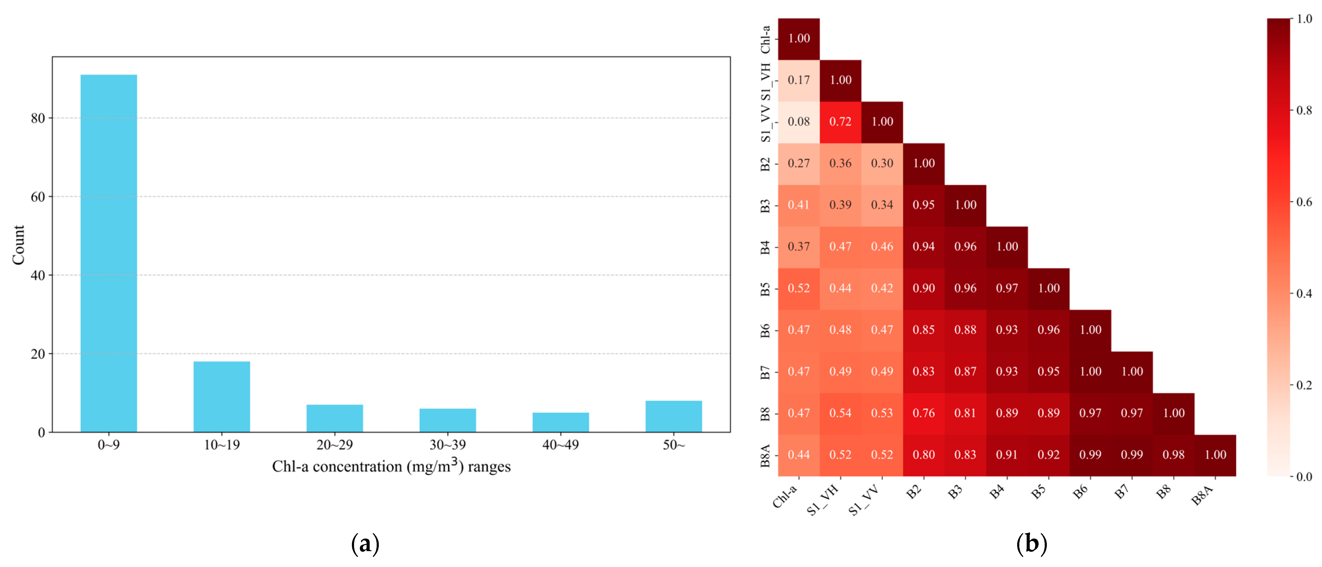
3.1. Characteristics of the Chl-a Retrieval Algorithm Datasets

In this study, datasets were constructed for CNN model training and evaluation, consisting of 135 samples (

Table A1. Sentinel-1/2 and Chl-a concentration acquisitions used for the construction of the dataset. The mean and standard deviation of Chl-a measured on the same date as the Sentinel-1/2 imagery acquisition are presented in ‘mean (standard deviation)’ format.

Image Date	Sentinel-1 Relative Orbit Number	Sentinel-2 Tile ID	No. of Samples	No. of Lakes	Chl-a (mg/m3)
28 January 2019	54	T52SCG T52SDF	4	3	5.93 (11.38)
3 April 2019	127	T52SCG T52SBF T52SDE T52SBD	12	4	7.15 (22.21)
3 May 2019	134	T52SCE T52SCH T52SDF	9	4	2.09 (3.25)
2 July 2019	134	T52SBF T52SCF	5	3	46 (1552.63)
1 August 2019	127	T52SCF	2	1	3 (2)
8 August 2019	54	T52SDG	1	1	64.6
30 September 2019	127	T52SBF T52SDF	4	2	104.43 (9310.18)
6 November 2019	61	T52SDE T52SDD	7	3	9.29 (52.50)
11 November 2019	134	T52SDD	2	1	1.05 (0.604)
4 February 2020	54	T52SDE	2	2	0.95 (1.13)
5 March 2020	61	T52SDF	2	1	1 (0.02)
23 March 2020	54	T52SCG T52SCF T52SDF	11	5	17.07 (102.62)
8 June 2020	127	T52SDF	1	1	1.1
25 August 2020	134	T52SCF T52SCE	8	3	17.3 (277.72)
6 October 2020	127	T52SDE	3	1	1.17 0.04)
23 November 2020	127	T52SCF T52SCD T52SDG	3	3	3.93 (9.16)
4 January 2021	134	T52SDF	1	1	1.1
3 February 2021	127	T52SDF	1	1	1.1
18 March 2021	54	T52SCH	3	1	1.07 (0.30)
23 March 2021	127	T52SCG	1	1	3.4
21 June 2021	134	T52SCH T52SCG	7	2	16.31 (227.26)
21 July 2021	127	T52SBF	4	2	82.73 (6106.68)
19 October 2021	134	T52SCD	1	1	6.2
17 January 2022	127	T52SDG	1	1	1.9
24 January 2022	54	T52SDG	1	1	1.7
17 May 2022	127	T52SCD T52SDF	2	2	1.6 (0.02)
8 November 2022	54	T52SCG T52SDE	6	3	1.87 (8.53)
13 March 2023	127	T52SDF T52SCG T52SCF	8	4	16.68 (249.75)
20 March 2023	54	T52SCF	1	1	5.7
8 November 2023	127	T52SDF T52SDD	4	2	1.65 (0.04)
20 November 2023	127	T52SDF	1	1	1.6
7 March 2024	127	T52SBF	1	1	31
5 July 2024	127	T52SCG	1	1	0.4
3 September 2024	127	T52SCF	12	1	32.27 (39.40)
10 September 2024	54	T52SDG T52SDE	3	8	17.48 (1520.31)

). The majority of the samples (91) had low Chl-a concentrations, ranging from 0 to 9 mg/m³, while only five samples had Chl-a concentrations between 40 and 49 mg/m³, making this concentration range the least common (Figure 4a). As Chl-a concentrations increased, the number of corresponding samples decreased, with fewer samples available for concentrations of 50 mg/m³ or higher. The Chl-a concentrations exhibited a positive correlation (ranging from 0.27 to 0.52) with reflectance values from the eight Sentinel-2 spectral bands (B2 to B8, B8A) (Figure 4b). Among these, the reflectance of the visible spectral bands (B2, B3, and B4) showed a lower correlation with Chl-a concentrations compared with near-infrared and red-edge bands. In contrast, the VH polarization data from Sentinel-1 displayed a weak correlation with Chl-a concentrations (r = 0.17), while the VV polarization data exhibited an even lower correlation (r = 0.08).

3.2. Performance of the Chl-a Retrieval Algorithm

In optimizing CNN model A, the configuration of the layers was as follows: the first and second convolutional layers each comprised 120 filters, the third and fourth convolutional layers each contained 80 filters, and the fifth convolutional layer utilized 72 filters (

Table 4. The layer information of each optimized CNN structure. For CNN 2D layers, values are displayed as (input channel, output channel), while linear layers are represented as (input feature, output feature).

Layer	Model A	Model B
Conv2D + ReLU + Batch normalization	(10, 120)	(8, 88)
Conv2D + ReLU + Batch normalization	(120, 120)	(88, 88)
Conv2D + ReLU + Batch normalization	(120, 80)	(88, 56)
Conv2D + ReLU + Batch normalization	(80, 80)	(56, 56)
Conv2D + ReLU + Batch normalization	(80, 72)	(56, 32)
Flatten	(72, 72)	(32, 32)
Linear + ReLU	(72, 80)	(32, 56)
Linear + ReLU	(80, 120)	(56, 88)
Linear + ReLU	(120, 1)	(88, 1)

). The output feature of the first linear layer was set to 80, while the second linear layer had an output feature of 120. For CNN model B, the layer configuration was adjusted as follows: the first and second convolutional layers each comprised 88 filters, the third and fourth convolutional layers each contained 56 filters, and the fifth convolutional layer implemented 32 filters. The output features for the linear layers were set to 56 for the first and 88 for the second.

CNN Model A, which used both Sentinel-2 and Sentinel-1 data, did not show a significant difference in training performance compared with Model B, which used only Sentinel-2 data. The test performance of CNN Model A resulted in an R² of 0.7992, RMSE of 10.3282 mg/m³, RPD of 2.2315 and bias of −0.4360 mg/m³. For CNN Model B, the test performance yielded an R² of 0.7075, an RMSE of 12.4649 mg/m³, a RPD of 1.8439, and a bias of 0.1625 mg/m³. For the test dataset, CNN Model A outperformed Model B, achieving better results in R², RMSE, and RFD (

Table 5. Performance of CNN models.

	Model A		Model B
	Train	Test	Train	Test
R2	0.8958	0.7992	0.8939	0.7075
RMSE (mg/m3)	11.3303	10.3282	11.2962	12.4649
RPD	3.0604	2.2315	3.0696	1.8489
Bias (mg/m3)	−0.0529	−0.4360	0.6826	0.1625

). Bias assessment revealed that CNN model A consistently underestimated the target values, whereas CNN model B showed a systematic overestimation pattern. Both CNN models exhibited tendencies to underestimate Chl-a concentration values in the 0 to 50 mg/m³ range (Figure 5). However, there was a tendency to overestimate as the values approached mg/m³, and due to the higher magnitude of overestimation errors, CNN model B exhibited a positive bias value. Thus, Model A demonstrated a more balanced predictive performance, with reduced tendencies for both overestimation and underestimation compared with Model B.

3.3. Evaluation of Variable Importance

Analysis of variable importance in CNN model A using SHAP revealed high importance for bands B5, B8a, and B8 (Figure 6). Phytoplankton induces spectral reflectance peaks at approximately 700 nm due to the minimization of the combined absorption of water and phytoplankton [49], which explains the high variable importance of B5 (705 nm) in the Chl-a concentration model. The NIR region exhibits reduced interference from factors that disrupt phytoplankton spectral characteristics, such as suspended particulate matter and colored dissolved organic matter, accounting for the high variable importance observed in B8 and B8a bands located in this region [50]. Notably, VV and VH polarization data from Sentinel-1 demonstrated high variable importance despite showing a lower correlation with Chl-a concentration compared with bands B3, B6, and B7.

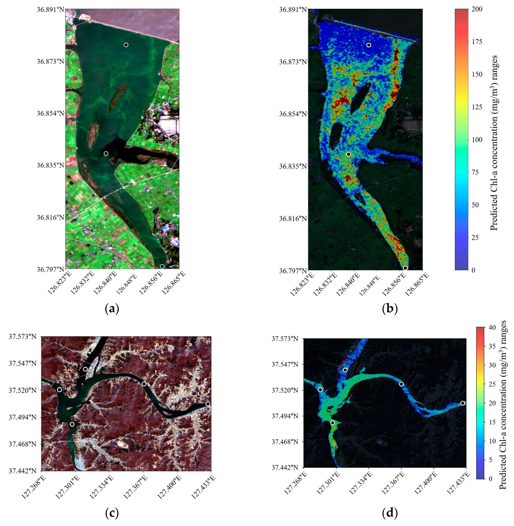
3.4. Spatial Distribution of Chl-a Concentration

The optimized CNN model A was applied to retrieve Chl-a concentrations in Sapgyo and Paldang Lakes in South Korea (Figure 7). On 30 September 2019, high Chl-a concentrations of 210 mg/m³ and 160.4 mg/m³ were recorded at sampling sites 2 and 3 in Sapgyo Lake, respectively. Based on coincident Sentinel-1 and Sentinel-2 imagery, the model-retrieved Chl-a concentrations at these sites were 150 mg/m³ and 143.2 mg/m³, respectively. Sampling site 1 in Sapgyo Lake recorded a lower Chl-a concentration of 41 mg/m³, which the model estimated to be 26.1 mg/m³. Overall, the model tended to underestimate Chl-a concentrations while successfully differentiating between high and low-concentration areas across the lake. On 23 March 2020, the lowest Chl-a concentration at Paldang Lake was recorded at sampling site 1, with a value of 6.9 mg/m³. Relatively high Chl-a concentrations (26.1 mg/m³, 18.5 mg/m³, 16.5 mg/m³, and 39.4 mg/m³, respectively) were observed at sampling sites 2 to 5. The model-based Chl-a retrieval results for these five sampling sites (7.8 mg/m³, 16.1 mg/m³, 12.3 mg/m³, 14.2 mg/m³, 23.2 mg/m³, respectively) also showed a tendency to underestimate, similar to the findings for Sapgyo Lake. CNN model A exhibited patterns consistent with the actual Chl-a concentration distributions in two lakes with distinct hydrological characteristics.

4. Discussion

4.1. Effect of SAR Data on Chl-a Retrieval

The performance of CNN Model A, which uses both Sentinel-1 SAR data and Sentinel-2 optical imagery as input variables, was compared with that of CNN Model B, which utilizes solely Sentinel-2 optical imagery. The training performance of CNN Model A was slightly higher than that of Model B, while its test performance was superior to that of Model B. The enhanced performance of CNN Model A appears to be due to the additional use of Sentinel-1 SAR data. Although the correlation between Sentinel-1 VV and VH polarization backscatter and Chl-a concentration was low, it cannot be concluded that variables with low correlation coefficients do not contribute to model performance [51]. Correlation coefficients fundamentally quantify linear relationships between variables and do not account for potential nonlinear associations [52]. However, since deep learning models like CNN can capture such nonlinear relationships through activation functions [53], even with low correlation, Sentinel-1 VV and VH polarization data may contribute to performance improvement. Indeed, SHAP analysis revealed that Sentinel-1 VV and VH polarization data exhibited higher variable importance than some optical band data that had shown a high correlation with Chl-a concentration. This result reflects the model’s ability to capture radar backscattering properties. Biological surfactants released by algae, which are the source of Chl-a, reduce both water surface tension and radar wave backscattering [54].

4.2. Evaluation of SAR and Optical Imagery-Based Remote Monitoring

As shown in Figure 7b, Sapgyo Lake, where Chl-a concentrations were estimated, features major inflow streams such as the Sapgyocheon and the Gokgyocheon, as well as a breakwater to block tidal currents. On 30 September 2019, when remote monitoring was conducted, high Chl-a concentrations were measured at sampling site 3 in Sapgyo Lake, where the Sapgyocheon flows into the lake, and at sampling site 2, where the Gokgyocheon mixes with the lake. In contrast, low Chl-a concentrations were observed at sampling site 1 in Sapgyo Lake, near the breakwater. Model A-based Chl-a retrieval results showed that high concentrations were estimated near sampling sites 2 and 3 in Sapgyo Lake, while low concentrations were estimated near sampling site 1. The model distinguished between high and low-concentration areas but tended to underestimate Chl-a concentrations overall. This underestimation appears to be due to the limited amount of data above 50 mg/m³ in the training dataset. It is expected that this bias will be addressed if the data imbalance in the training dataset is corrected [55]. Another cause of underestimation is attributed to the ‘packaging effect,’ wherein pigments are highly concentrated within phytoplankton cells, resulting in decreased light absorption efficiency [56]. On the other hand, Paldang Lake has three inflow streams—the Gyeongancheon, the Bukhangang River, and the Namhangang River— each of which has different water quality characteristics, as shown in Figure 7d. On 23 March 2020, when remote sensing monitoring was conducted, the highest Chl-a concentration was recorded at sampling site 5 in the Gyeongancheon inflow area of Paldang Lake. In contrast, the lowest Chl-a concentration was observed at sampling site 2, located near the water gate. This was followed by sampling site 3, situated at the location where the Namhangang flows into the lake, and sampling site 4, where the Bukhangang enters Paldang Lake. Sampling site 1 in Paldang Lake, located where the Namhangang flows into the lake, was positioned relatively far from Paldang Lake compared with the other four sampling sites, resulting in the lowest Chl-a concentration. Within Paldang Lake, CNN Model A successfully differentiated between areas with high and low concentrations based on in situ measurements, although it tended to underestimate the concentration. Therefore, in future studies, resolving data imbalances by acquiring additional data from high-concentration areas and increasing the diversity of training data seems to enhance the accuracy of remote sensing-based Chl-a monitoring.

4.3. Effect of Small Dataset on Model Performance

While deep learning models such as CNNs demonstrate superior performance when trained on large datasets, they risk overfitting when applied to limited training data [57]. In this study, we collected 135 samples of concurrent data from Sentinel-1/2 and Chl-a concentration measurements with varying temporal resolutions. Applying CNN models to this relatively small dataset of 135 samples presents a risk of overfitting. Nevertheless, we determined that deep learning approaches like CNNs are more suitable than traditional machine learning methods for analyzing the complex relationship between SAR data and Chl-a concentrations [58]. To mitigate potential overfitting, we incorporated batch normalization layers into our CNN architecture [59]. However, it is important to acknowledge that batch normalization alone cannot completely eliminate the risk of overfitting. Given our data constraints, future work should explore additional techniques such as data augmentation, semi-supervised learning [60], and self-supervised learning methods [61], which are specifically designed for scenarios with limited labeled data.

5. Conclusions

In this study, to evaluate the effectiveness of SAR data for Chl-a retrieval based on remote sensing, a CNN, designated as Model A, was developed using both Sentinel-1 SAR data and Sentinel-2 optical imagery as input variables for 35 lakes across South Korea. Its performance was compared with that of CNN Model B, which was trained using only Sentinel-2 optical imagery as input variables. On the test dataset, Model A demonstrated superior performance (R² = 0.7992, RMSE = 10.3282 mg/m³, RPD = 2.2315) compared with Model B (R² = 0.7075, RMSE = 12.4649 mg/m³, RPD = 1.8439). Additionally, the variable importance of Model A showed moderate contributions from Sentinel-1 VV (0.96) and VH (0.71) among all variables. These results suggest that incorporating Sentinel-1 SAR data can significantly enhance the performance of Chl-a retrieval models.

However, this study has a main limitation. Model A was trained on a relatively small and imbalanced dataset (91 samples) with a limited representation of high Chl-a concentrations. Consequently, the model tended to underestimate Chl-a concentrations across studied lakes. Future research should focus on expanding the training dataset and addressing class imbalance to enhance the accuracy of remote sensing-based Chl-a monitoring. Despite these limitations, this study demonstrates improved Chl-a retrieval performance through SAR data integration, providing a foundational reference for future research utilizing combined SAR and optical remote sensing approaches.

References

1. Zhang, Y.; Hallikainen, M.; Zhang, H.; Duan, H.; Li, Y.; San Liang, X. Chlorophyll-a estimation in turbid waters using combined SAR Data with hyperspectral reflectance Data: A case study in Lake Taihu, China. IEEE J. Sel. Top. Appl. Earth Obs. Remote Sens. 2018, 11, 1325–1336. [Google Scholar] [CrossRef]
2. Xiong, J.; Lin, C.; Cao, Z.; Hu, M.; Xue, K.; Chen, X.; Ma, R. Development of remote sensing algorithm for total phosphorus concentration in eutrophic lakes: Conventional or machine learning? Water Res. 2022, 215, 118213. [Google Scholar] [CrossRef] [PubMed]
3. Ayele, H.S.; Atlabachew, M. Review of characterization, factors, impacts, and solutions of Lake eutrophication: Lesson for lake Tana, Ethiopia. Environ. Sci. Pollut. Res. 2021, 28, 14233–14252. [Google Scholar] [CrossRef] [PubMed]
4. Dodds, W.K.; Bouska, W.W.; Eitzmann, J.L.; Pilger, T.J.; Pitts, K.L.; Riley, A.J.; Schloesser, J.T.; Thornbrugh, D.J. Eutrophication of US freshwaters: Analysis of potential economic damages. Environ. Sci. Technol. 2009, 43, 12–19. [Google Scholar] [CrossRef]
5. Riza, M.; Ehsan, M.N.; Pervez, M.N.; Khyum, M.M.O.; Cai, Y.; Naddeo, V. Control of eutrophication in aquatic ecosystems by sustainable dredging: Effectiveness, environmental impacts, and implications. Case Stud. Chem. Environ. Eng. 2023, 7, 100297. [Google Scholar] [CrossRef]
6. Kim, H.G.; Hong, S.; Chon, T.-S.; Joo, G.-J. Spatial patterning of chlorophyll a and water-quality measurements for determining environmental thresholds for local eutrophication in the Nakdong River basin. Environ. Pollut. 2021, 268, 115701. [Google Scholar] [CrossRef]
7. Suresh, K.; Tang, T.; Van Vliet, M.T.; Bierkens, M.F.; Strokal, M.; Sorger-Domenigg, F.; Wada, Y. Recent advancement in water quality indicators for eutrophication in global freshwater lakes. Environ. Res. Lett. 2023, 18, 063004. [Google Scholar] [CrossRef]
8. Duan, H.; Zhang, Y.; Zhang, B.; Song, K.; Wang, Z. Assessment of chlorophyll-a concentration and trophic state for Lake Chagan using Landsat TM and field spectral data. Environ. Monit. Assess. 2007, 129, 295–308. [Google Scholar] [CrossRef]
9. Chen, C.; Chen, Q.; Li, G.; He, M.; Dong, J.; Yan, H.; Wang, Z.; Duan, Z. A novel multi-source data fusion method based on Bayesian inference for accurate estimation of chlorophyll-a concentration over eutrophic lakes. Environ. Model. Softw. 2021, 141, 105057. [Google Scholar] [CrossRef]
10. Park, J.; Khanal, S.; Zhao, K.; Byun, K. Remote sensing of chlorophyll-a and water quality over Inland Lakes: How to alleviate geo-location error and temporal discrepancy in model training. Remote Sens. 2024, 16, 2761. [Google Scholar] [CrossRef]
11. Yang, Z.; Reiter, M.; Munyei, N. Estimation of chlorophyll-a concentrations in diverse water bodies using ratio-based NIR/Red indices. Remote Sens. Appl. Soc. Environ. 2017, 6, 52–58. [Google Scholar] [CrossRef]
12. Gons, H.J.; Auer, M.T.; Effler, S.W. MERIS satellite chlorophyll mapping of oligotrophic and eutrophic waters in the Laurentian Great Lakes. Remote Sens. Environ. 2008, 112, 4098–4106. [Google Scholar] [CrossRef]
13. Dall’Olmo, G.; Gitelson, A.A. Effect of bio-optical parameter variability on the remote estimation of chlorophyll-a concentration in turbid productive waters: Experimental results. Appl. Opt. 2005, 44, 412–422. [Google Scholar] [CrossRef] [PubMed]
14. Jiang, W.; Knight, B.R.; Cornelisen, C.; Barter, P.; Kudela, R. Simplifying regional tuning of MODIS algorithms for monitoring chlorophyll-a in coastal waters. Front. Mar. Sci. 2017, 4, 151. [Google Scholar] [CrossRef]
15. Cao, Q.; Yu, G.; Sun, S.; Dou, Y.; Li, H.; Qiao, Z. Monitoring water quality of the Haihe River based on ground-based hyperspectral remote sensing. Water 2021, 14, 22. [Google Scholar] [CrossRef]
16. Cao, Z.; Ma, R.; Duan, H.; Pahlevan, N.; Melack, J.; Shen, M.; Xue, K. A machine learning approach to estimate chlorophyll-a from Landsat-8 measurements in inland lakes. Remote Sens. Environ. 2020, 248, 111974. [Google Scholar] [CrossRef]
17. Ha, N.T.T.; Thao, N.T.P.; Koike, K.; Nhuan, M.T. Selecting the best band ratio to estimate chlorophyll-a concentration in a tropical freshwater lake using sentinel 2A images from a case study of Lake Ba Be (Northern Vietnam). ISPRS Int. J. Geo-Inf. 2017, 6, 290. [Google Scholar] [CrossRef]
18. Pyo, J.; Hong, S.M.; Jang, J.; Park, S.; Park, J.; Noh, J.H.; Cho, K.H. Drone-borne sensing of major and accessory pigments in algae using deep learning modeling. GIScience Remote Sens. 2022, 59, 310–332. [Google Scholar] [CrossRef]
19. Llodrà-Llabrés, J.; Martínez-López, J.; Postma, T.; Pérez-Martínez, C.; Alcaraz-Segura, D. Retrieving water chlorophyll-a concentration in inland waters from Sentinel-2 imagery: Review of operability, performance and ways forward. Int. J. Appl. Earth Obs. Geoinf. 2023, 125, 103605. [Google Scholar] [CrossRef]
20. Shen, M.; Luo, J.; Cao, Z.; Xue, K.; Qi, T.; Ma, J.; Liu, D.; Song, K.; Feng, L.; Duan, H. Random forest: An optimal chlorophyll-a algorithm for optically complex inland water suffering atmospheric correction uncertainties. J. Hydrol. 2022, 615, 128685. [Google Scholar] [CrossRef]
21. Wu, L.; Sun, M.; Min, L.; Zhao, J.; Li, N.; Guo, Z. An improved method of algal-bloom discrimination in Taihu Lake using Sentinel-1A data. In Proceedings of the 2019 6th Asia-Pacific Conference on Synthetic Aperture Radar (APSAR), Xiamen, China, 26–29 November 2019; pp. 1–5. [Google Scholar]
22. Zahir, M.; Su, Y.; Shahzad, M.I.; Ayub, G.; Rehman, S.U.; Ijaz, J. A review on monitoring, forecasting, and early warning of harmful algal bloom. Aquaculture 2024, 593, 741351. [Google Scholar] [CrossRef]
23. Gao, L.; Li, X.; Kong, F.; Yu, R.; Guo, Y.; Ren, Y. AlgaeNet: A deep-learning framework to detect floating green algae from optical and SAR imagery. IEEE J. Sel. Top. Appl. Earth Obs. Remote Sens. 2022, 15, 2782–2796. [Google Scholar] [CrossRef]
24. Lavrova, O.Y.; Mityagina, M. Manifestation specifics of hydrodynamic processes in satellite images of intense phytoplankton bloom areas. Izv. Atmos. Ocean. Phys. 2016, 52, 974–987. [Google Scholar] [CrossRef]
25. Xin, Y.; Luo, J.; Xu, Y.; Sun, Z.; Qi, T.; Shen, M.; Qiu, Y.; Xiao, Q.; Huang, L.; Zhao, J. SSAVI-GMM: An automatic algorithm for mapping submerged aquatic vegetation in shallow lakes using Sentinel-1 SAR and Sentinel-2 MSI data. IEEE Trans. Geosci. Remote Sens. 2024, 62, 4416610. [Google Scholar] [CrossRef]
26. Cen, H.; Jiang, J.; Han, G.; Lin, X.; Liu, Y.; Jia, X.; Ji, Q.; Li, B. Applying deep learning in the prediction of chlorophyll-a in the East China Sea. Remote Sens. 2022, 14, 5461. [Google Scholar] [CrossRef]
27. Hamze-Ziabari, S.M.; Foroughan, M.; Lemmin, U.; Barry, D.A. Monitoring mesoscale to submesoscale processes in large lakes with Sentinel-1 SAR imagery: The case of Lake Geneva. Remote Sens. 2022, 14, 4967. [Google Scholar] [CrossRef]
28. Qi, L.; Wang, M.; Hu, C.; Holt, B. On the capacity of Sentinel-1 synthetic aperture radar in detecting floating macroalgae and other floating matters. Remote Sens. Environ. 2022, 280, 113188. [Google Scholar] [CrossRef]
29. Kim, J.; Lee, T.; Seo, D. Algal bloom prediction of the lower Han River, Korea using the EFDC hydrodynamic and water quality model. Ecol. Model. 2017, 366, 27–36. [Google Scholar] [CrossRef]
30. Shin, J.; Lee, G.; Kim, T.; Cho, K.H.; Hong, S.M.; Kwon, D.H.; Pyo, J.; Cha, Y. Deep learning-based efficient drone-borne sensing of cyanobacterial blooms using a clique-based feature extraction approach. Sci. Total Environ. 2024, 912, 169540. [Google Scholar] [CrossRef]
31. Lee, S.; Choi, B.; Kim, S.J.; Kim, J.; Kang, D.; Lee, J. Relationship between freshwater harmful algal blooms and neurodegenerative disease incidence rates in South Korea. Environ. Health 2022, 21, 116. [Google Scholar] [CrossRef]
32. Kim, Y.W.; Kim, T.; Shin, J.; Lee, D.-S.; Park, Y.-S.; Kim, Y.; Cha, Y. Validity evaluation of a machine-learning model for chlorophyll a retrieval using Sentinel-2 from inland and coastal waters. Ecol. Indic. 2022, 137, 108737. [Google Scholar] [CrossRef]
33. Seo, A.; Lee, K.; Kim, B.; Choung, Y. Classifying plant species indicators of eutrophication in Korean lakes. Paddy Water Environ. 2014, 12, 29–40. [Google Scholar] [CrossRef]
34. Gomarasca, M.A.; Tornato, A.; Spizzichino, D.; Valentini, E.; Taramelli, A.; Satalino, G.; Vincini, M.; Boschetti, M.; Colombo, R.; Rossi, L. Sentinel for applications in agriculture. Int. Arch. Photogramm. Remote Sens. Spat. Inf. Sci. 2019, 42, 91–98. [Google Scholar] [CrossRef]
35. Filipponi, F. Sentinel-1 GRD Preprocessing Workflow. Proceedings 2019, 18, 11. [Google Scholar] [CrossRef]
36. Phiri, D.; Simwanda, M.; Salekin, S.; Nyirenda, V.R.; Murayama, Y.; Ranagalage, M. Sentinel-2 data for land cover/use mapping: A review. Remote Sens. 2020, 12, 2291. [Google Scholar] [CrossRef]
37. Sola, I.; García-Martín, A.; Sandonís-Pozo, L.; Álvarez-Mozos, J.; Pérez-Cabello, F.; González-Audícana, M.; Llovería, R.M. Assessment of atmospheric correction methods for Sentinel-2 images in Mediterranean landscapes. Int. J. Appl. Earth Obs. Geoinf. 2018, 73, 63–76. [Google Scholar] [CrossRef]
38. Kwong, I.H.; Wong, F.K.; Fung, T. Automatic mapping and monitoring of marine water quality parameters in Hong Kong using Sentinel-2 image time-series and Google Earth Engine cloud computing. Front. Mar. Sci. 2022, 9, 871470. [Google Scholar] [CrossRef]
39. Bhatt, D.; Patel, C.; Talsania, H.; Patel, J.; Vaghela, R.; Pandya, S.; Modi, K.; Ghayvat, H. CNN variants for computer vision: History, architecture, application, challenges and future scope. Electronics 2021, 10, 2470. [Google Scholar] [CrossRef]
40. Alzubaidi, L.; Zhang, J.; Humaidi, A.J.; Al-Dujaili, A.; Duan, Y.; Al-Shamma, O.; Santamaría, J.; Fadhel, M.A.; Al-Amidie, M.; Farhan, L. Review of deep learning: Concepts, CNN architectures, challenges, applications, future directions. J. Big Data 2021, 8, 53. [Google Scholar] [CrossRef]
41. Segal-Rozenhaimer, M.; Li, A.; Das, K.; Chirayath, V. Cloud detection algorithm for multi-modal satellite imagery using convolutional neural-networks (CNN). Remote Sens. Environ. 2020, 237, 111446. [Google Scholar] [CrossRef]
42. Song, J.; Gao, S.; Zhu, Y.; Ma, C. A survey of remote sensing image classification based on CNNs. Big Earth Data 2019, 3, 232–254. [Google Scholar] [CrossRef]
43. Xue, M.; Hang, R.; Liu, Q.; Yuan, X.-T.; Lu, X. CNN-based near-real-time precipitation estimation from Fengyun-2 satellite over Xinjiang, China. Atmos. Res. 2021, 250, 105337. [Google Scholar] [CrossRef]
44. Li, F.; Wang, L.; Liu, J.; Wang, Y.; Chang, Q. Evaluation of leaf N concentration in winter wheat based on discrete wavelet transform analysis. Remote Sens. 2019, 11, 1331. [Google Scholar] [CrossRef]
45. Watanabe, F.; Alcântara, E.; Imai, N.; Rodrigues, T.; Bernardo, N. Estimation of chlorophyll-a concentration from optimizing a semi-analytical algorithm in productive inland waters. Remote Sens. 2018, 10, 227. [Google Scholar] [CrossRef]
46. Mosca, E.; Szigeti, F.; Tragianni, S.; Gallagher, D.; Groh, G. SHAP-based explanation methods: A review for NLP interpretability. In Proceedings of the 29th International Conference on Computational Linguistics, Gyeongju, Republic of Korea, 12–17 October 2022; pp. 4593–4603. [Google Scholar]
47. Zhang, J.; Ma, X.; Zhang, J.; Sun, D.; Zhou, X.; Mi, C.; Wen, H. Insights into geospatial heterogeneity of landslide susceptibility based on the SHAP-XGBoost model. J. Environ. Manag. 2023, 332, 117357. [Google Scholar] [CrossRef]
48. Lundberg, S.M.; Lee, S.-I. A unified approach to interpreting model predictions. In Advances in Neural Information Processing Systems, Proceedings of the NIPS’17: Proceedings of the 31st International Conference on Neural Information Processing Systems, Long Beach, CA, USA, 4–9 December 2017; Curran Associates Inc.: Red Hook, NY, USA, 2017; Volume 30. [Google Scholar]
49. Bramich, J.; Bolch, C.J.; Fischer, A. Improved red-edge chlorophyll-a detection for Sentinel 2. Ecol. Indic. 2021, 120, 106876. [Google Scholar] [CrossRef]
50. Tran, M.D.; Vantrepotte, V.; Loisel, H.; Oliveira, E.N.; Tran, K.T.; Jorge, D.; Mériaux, X.; Paranhos, R. Band ratios combination for estimating chlorophyll-a from sentinel-2 and sentinel-3 in coastal waters. Remote Sens. 2023, 15, 1653. [Google Scholar] [CrossRef]
51. Gregorutti, B.; Michel, B.; Saint-Pierre, P. Correlation and variable importance in random forests. Stat. Comput. 2017, 27, 659–678. [Google Scholar] [CrossRef]
52. Janse, R.J.; Hoekstra, T.; Jager, K.J.; Zoccali, C.; Tripepi, G.; Dekker, F.W.; Van Diepen, M. Conducting correlation analysis: Important limitations and pitfalls. Clin. Kidney J. 2021, 14, 2332–2337. [Google Scholar] [CrossRef]
53. Namatēvs, I. Deep convolutional neural networks: Structure, feature extraction and training. Inf. Technol. Manag. Sci. 2017, 20, 40–47. [Google Scholar] [CrossRef]
54. Zhang, T.; Hu, H.; Ma, X.; Zhang, Y. Long-term spatiotemporal variation and environmental driving forces analyses of algal blooms in Taihu Lake based on multi-source satellite and land observations. Water 2020, 12, 1035. [Google Scholar] [CrossRef]
55. Kowatsch, D.; Müller, N.M.; Tscharke, K.; Sperl, P.; Bötinger, K. Imbalance in Regression Datasets. arXiv 2024, arXiv:2402.11963. [Google Scholar] [CrossRef]
56. Szeto, M.; Werdell, P.; Moore, T.; Campbell, J. Are the world’s oceans optically different? J. Geophys. Res. Ocean. 2011, 116, C00H04. [Google Scholar] [CrossRef]
57. Pasupa, K.; Sunhem, W. A comparison between shallow and deep architecture classifiers on small dataset. In Proceedings of the 2016 8th International Conference on Information Technology and Electrical Engineering (ICITEE), Yogyakarta, Indonesia, 5–6 October 2016; pp. 1–6. [Google Scholar]
58. Janiesch, C.; Zschech, P.; Heinrich, K. Machine learning and deep learning. Electron. Mark. 2021, 31, 685–695. [Google Scholar] [CrossRef]
59. Ioffe, S.; Szegedy, C. Batch normalization: Accelerating deep network training by reducing internal covariate shift. In Proceedings of the 32nd International Conference on Machine Learning, Lille, France, 7–9 July 2015; pp. 448–456. [Google Scholar]
60. Shi, X.; Gu, L.; Li, X.; Jiang, T.; Gao, T. Automated spectral transfer learning strategy for semi-supervised regression on Chlorophyll-a retrievals with Sentinel-2 imagery. Int. J. Digit. Earth 2024, 17, 2313856. [Google Scholar] [CrossRef]
61. Rani, V.; Nabi, S.T.; Kumar, M.; Mittal, A.; Kumar, K. Self-supervised learning: A succinct review. Arch. Comput. Methods Eng. 2023, 30, 2761–2775. [Google Scholar] [CrossRef]
Figure 1. Study flow for Chl-a retrieval algorithm.
Water 17 01718 g001
Figure 2. Study area. Red dots indicate the location of lakes used in the research.
Water 17 01718 g002
Figure 3. Architecture of CNN model for retrieval of Chl-a.
Water 17 01718 g003
Figure 4. Data characteristics. (a) Data distribution by Chl-a concentration intervals; (b) Correlation coefficients between Chl-a concentration and Sentinel-1, 2 variables.
Water 17 01718 g004
Figure 5. Comparisons between observed and predicted Chl-a concentration using (a) CNN model A and (b) CNN model B. The green dashed line represents the 1:1 line.
Water 17 01718 g005
Figure 6. Variable importance of CNN model A on (a) training data and (b) test data.
Water 17 01718 g006
Figure 7. Sentinel-2 imagery and corresponding Chl-a concentration estimation results. (a) Sentinel-2 image of Sapgyo Lake on 30 September 2019; (b) Chl-a concentration estimation results for Sapgyoho on 30 September 2019; (c) Sentinel-2 image of Paldang Lake on 23 March 2020; (d) Chl-a concentration estimation results for Paldangho on 23 March 2020.
Water 17 01718 g007