Abstract
Accurate estimation of soil moisture content (SMC) is crucial for effective water management, enabling improved monitoring of water stress and a deeper understanding of hydrological processes. While satellite remote sensing provides broad coverage, its spatial resolution often limits its ability to capture small-scale variations in SMC, especially in landscapes with diverse land-cover types. Unmanned aerial vehicles (UAVs) equipped with hyperspectral sensors offer a promising solution to overcome this limitation. This study compares the effectiveness of Sentinel-2, Landsat-8/9 multispectral data and UAV hyperspectral data (from 339.6 nm to 1028.8 nm with spectral bands) in estimating SMC in a research farm consisting of bare soil, cropland and grassland. A DJI Matrice 100 UAV equipped with a hyperspectral spectrometer collected data on 14 field campaigns, synchronized with satellite overflights. Five machine-learning algorithms including extreme learning machines (ELMs), Gaussian process regression (GPR), partial least squares regression (PLSR), support vector regression (SVR) and artificial neural network (ANN) were used to estimate SMC, focusing on the influence of land cover on the accuracy of SMC estimation. The findings indicated that GPR outperformed the other models when using Landsat-8/9 and hyperspectral photography data, demonstrating a tight correlation with the observed SMC (R2 = 0.64 and 0.89, respectively). For Sentinel-2 data, ELM showed the highest correlation, with an R2 value of 0.46. In addition, a comparative analysis showed that the UAV hyperspectral data outperformed both satellite sources due to better spatial and spectral resolution. In addition, the Landsat-8/9 data outperformed the Sentinel-2 data in terms of SMC estimation accuracy. For the different land-cover types, all types of remote-sensing data showed the highest accuracy for bare soil compared to cropland and grassland. This research highlights the potential of integrating UAV-based spectroscopy and machine-learning techniques as complementary tools to satellite platforms for precise SMC monitoring. The findings contribute to the further development of remote-sensing methods and improve the understanding of SMC dynamics in heterogeneous landscapes, with significant implications for precision agriculture. By enhancing the SMC estimation accuracy at high spatial resolution, this approach can optimize irrigation practices, improve cropping strategies and contribute to sustainable agricultural practices, ultimately enabling better decision-making for farmers and land managers. However, its broader applicability depends on factors such as scalability and performance under different conditions.
1. Introduction
Soil moisture content (SMC) is a critical variable for understanding climate and hydrological processes warranting investigation due to its dynamic temporal and spatial variations [1]. SMC significantly influences water distribution among different hydrological cycle components [2,3,4]. In agriculture, monitoring water stress and forecasting crop yields depend on precise measurement of SMC at various plant growth stages [5,6].
In contrast to field-based methods to measure SMC, remote-sensing technology enables the large-scale estimation of SMC and thus offers significant opportunities for spatial planning [7,8,9]. The effectiveness of various satellite-based imaging techniques, including optical, thermal, active and passive microwave sensors, in estimating SMC is well established [9,10,11]. However, each imaging modality has specific advantages and limitations, and no single approach can fully meet the combined requirements of spatial, spectral and temporal resolution. For bare soil, SMC estimation is usually based on detecting changes in soil color, as wet soil is characterized by a darker shade and lower reflectivity compared to dry soil [12,13]. In regions with vegetation cover, however, additional considerations are required. These considerations include the analysis of vegetation reflectance caused by SMC and canopy shade. The spectral signature of a vegetation canopy provides important insights into growth state and overall health, with distinct changes in spectral characteristics observed under varying levels of SMC stress [6]. Nevertheless, estimating SMC in heterogeneous regions remains particularly challenging due to the complex interplay of land cover and soil variability. Specific factors contributing to this complexity include topographic variability, which affects drainage and water retention, crop heterogeneity, which affects canopy structure and evapotranspiration patterns, and soil texture, which determines the soil’s ability to retain and transmit moisture. To improve accuracy, it is important to identify the most appropriate remote-sensing data sources and develop robust modeling approaches.
Machine-learning algorithms have proven successful in creating predictive models from extensive remote-sensing datasets, enabling detailed analyses of spatial and temporal environmental changes [14]. Many studies have shown the considerable potential of machine learning for retrieving SMC from satellite data [15,16,17,18]. In a study by Rabiei et al. [19], Sentinel-2 optical images and Sentinel-1 Synthetic Aperture Radar (SAR) were utilized to estimate SMC using linear regression, convolutional neural network (CNN), and multilayer perceptron models. Thermal and optical data from Landsat-8 were used by Adab et al. [15] to estimate SMC in areas with different land-use patterns using elastic net regression, artificial neural network (ANN), Random Forest and support vector machine algorithms. In another study, SMC estimation was performed using Random Forest, Linear Regression and Extra Tree with satellite data from Landsat-8, GF-1 and GF-4 [20], and more accurate SMC estimates were obtained at depths of 0.03 and 0.1 m than at 0.2 m, especially in densely vegetated areas. In a study by Wang et al. [21], the NDVI and NDWI indices from Sentinel-2, Landsat-8 and GF-1 satellites were compared to estimate SMC in a region of China where winter wheat and corn are predominantly grown. The results showed that the data from Sentinel-2 provided more accurate SMC estimates in agricultural areas than those from the other two satellites. Liu et al. [22] have also shown that Sentinel-2 imagery performs robustly in estimating SMC even in areas with vegetation coverage. However, the accuracy of SMC estimates derived from Landsat-8 data was found to decrease with increasing vegetation cover, as noted by Mobasheri and Amani [23].
Satellites such as Sentinel-2 provide valuable data for estimating SMC in vegetated areas, especially due to their red-edge bands, which are sensitive to vegetation stress and water content. However, satellite imagery is often limited by its spectral and spatial resolution. In contrast, unmanned aerial vehicles (UAVs) offer much higher spatial and spectral resolution, making them a valuable complement to satellites for detailed and accurate observations [24]. While UAVs provide high-resolution data for SMC estimates, their use also brings practical challenges. These include high operating costs, legal and logistical constraints and sensitivity to weather conditions. These practical limitations need to be carefully considered when collecting data in real-world applications. Recent studies have increasingly integrated UAVs with multispectral sensors [18,25,26,27] and hyperspectral sensors [17,24,28] to improve SMC estimation. Cheng et al. [29] used a UAV equipped with thermal, RGB and multispectral sensors, demonstrating that SMC estimation was most accurate in corn fields in regions with 20–40% canopy cover. Similarly, Luo et al. [30] combined Radarsat-2, Landsat-8 and digital elevation model (DEM) data from UAVs and ASTER to estimate the SMC in heterogeneous areas, finding that the infrared and optical bands from Landsat-8 together with DEM data extracted from UAVs showed a stronger correlation with the SMC compared to other datasets. In addition, Shokati et al. [18] highlighted the great potential of UAV-captured RGB data for accurate SMC estimation and emphasized the adaptability of UAV-based approaches.
Previous studies on SMC retrieval have relied primarily on point-based measurements (e.g., laboratory or on-site methods) or spaceborne spectroscopy data, while less attention has been paid to UAV-based spectroscopy despite its potential to provide higher spatial and spectral resolution for more precise SMC estimation [17,24,28]. In addition, the effect of land cover on the accuracy of different machine-learning models and remote-sensing data sources in estimating the SMC has not been sufficiently investigated. Therefore, this study aims to compare the performance of different machine-learning algorithms (i.e., ANN, SVR, PLSR, GPR and ELM) in estimating SMC using multi- and hyperspectral data from both satellite and UAV platforms, while evaluating the impact of different land-cover classes on the accuracy of these estimates. By addressing these gaps, this research aims to improve the understanding of SMC dynamics in heterogeneous environments and increase the applicability of remote-sensing and machine-learning techniques for more reliable SMC monitoring in diverse landscapes.
2. Materials and Methods
2.1. Study Area
A 100-hectare research farm at the University of Tehran, Iran, was selected as the study site (Figure 1). The farm is almost flat, with an elevation ranging between 980 and 990 m and an average elevation of 985 m. The mean annual temperature is 16 °C. The region has a distinct climate characterized by hot, sunny summers and cold, dry winters. The average annual rainfall is 217 mm, which leads to water shortage challenges in the region. Consequently, crop cultivation varies yearly and is influenced by water availability. Nevertheless, mainly alfalfa, wheat and maize remain the predominant crops. The agricultural parts of the farm rely on incidental surface irrigation, while the infertile areas depend solely on rainfall. The predominant soil texture is silty loam and the soils in the area are characterized by high electrical conductivity, indicating salinity issues. In addition, the region experiences high evapotranspiration rates, which further exacerbate water scarcity and affect crop productivity.
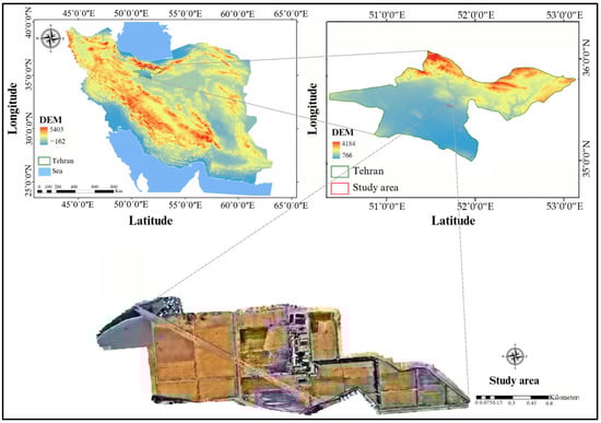
Figure 1.
Digital elevation model (DEM) and location of the study area.
2.2. Methodology
2.2.1. Workflow
Three primary phases make up the framework of the research (Figure 2): (1) data preprocessing, (2) model construction and evaluation, (3) analysis of the effects of land cover on the datasets and machine-learning models.
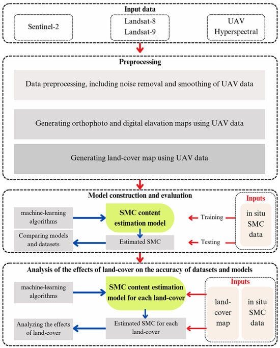
Figure 2.
Workflow of soil moisture content (SMC) retrieval with UAV-based spectroscopy and multispectral satellite imagery.
2.2.2. Field Measurements
Collection of Ground Truth Data
The data collection was conducted on 14 different dates between 6 September 2021 and 17 January 2023, from the soil surface at a depth of 0–5 cm. For each data collection, 45 points were randomly selected for soil sampling. Representative SMC values were determined using the five-diagonal-point method. In this approach, five soil samples were collected at each point, the average value of which was recorded as the total SMC value for the respective location. The soil sampling was timed to coincide with the collection of the multispectral and hyperspectral data. The samples were then dried in a laboratory oven at 105 °C for 24 h. The gravimetric analysis was then used to calculate the SMC percentage (Equation (1)).
where ω is the SMC percentage (%), is the weight of wet soil (gr) and is the weight of dry soil (gr).
Soil Analysis and Laboratory Work
Considering the impact of soil properties on surface spectral reflectance [31,32], 25 sampling points were selected in the study area to investigate the distribution of soil properties. Four important soil properties—texture, pH, electrical conductivity (EC) and color—were measured at these points (Figure S1). A pH meter and an EC meter were used to measure pH and electrical conductivity, respectively. The Munsell color book was used to evaluate soil color and the hydrometer technique was used to quantify soil texture [33].
2.2.3. Satellite Multispectral Data
Multispectral data acquired by Sentinel-2, Landsat-8 and Landsat-9 satellites with less than 10% cloud cover were used for this study. The Sentinel-2 Level-2A (L2A) surface reflectance images were downloaded from the European Space Agency website (https://copernicus.eu (accessed on 31 May 2023)). For the Landsat-8 and Landsat-9 data, Collection-2 Level-2 images were obtained from the United States Geological Survey website (https://earthexplorer.usgs.gov (accessed on 31 May 2023)). As these multispectral data had already undergone geometric and radiometric corrections, no further preprocessing steps were required. Because of the comparable specifications of the Landsat-8 and Landsat-9 satellites, they are collectively referred to as Landsat-8/9 in the following.
2.2.4. UAV Hyperspectral Data
Specifications of the UAV Equipped with Hyperspectral and RGB Sensors
This study also used hyperspectral data obtained with the CoSpectroCam sensor. CoSpectroCam is an optical coaxial system that combines an RGB camera with a spectrometer. The RGB camera provides images with a resolution of 700 × 800 pixels, while the spectrometer provides a high spectral resolution of 0.35 nm and covers a spectral range from 339.6 nm to 1028.8 nm with 2048 spectral bands. The spectrometer’s field of view (FOV) is represented as a rectangle superimposed on the RGB image, linking the spatial features captured by the RGB camera with the spectral features derived from the reflectance spectra (Figure 3). This FOV referred to as the “slit rectangle”, corresponds to the part of the image from which the spectrum is captured by the CoSpectroCam, rather than the entire image.
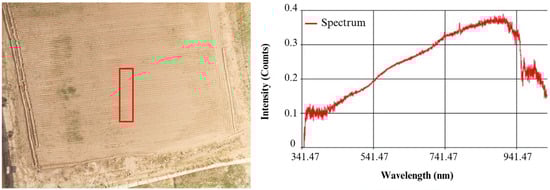
Figure 3.
Concept of the slit rectangle in the SpectroCam: The left panel shows a sample RGB image with the slit rectangle (the spectrometer’s field of view) in the center of the image, while the right panel shows the spectrum corresponding to the slit rectangle.
The aerial data of the region were captured by mounting the CoSpectroCam on a DJI Matrice 100 UAV (manufactured by DJI, headquartered in Shenzhen, China), which was also equipped with a Zenmuse Z3 RGB camera (manufactured by DJI, headquartered in Shenzhen, China) with a resolution of 3000 × 4000 pixels (Figure 4). In this study, hyperspectral data were captured using the CoSpectroCam, while RGB images were obtained from both the CoSpectroCam and the UAV’s RGB camera.
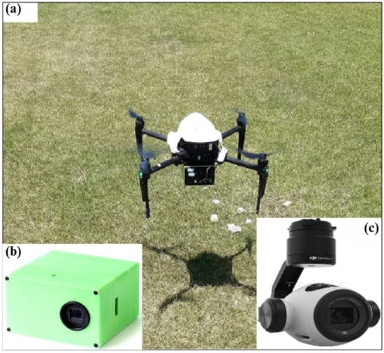
Figure 4.
(a) DJI Matrice 100 UAV equipped with CoSpectroCam and RGB sensors, (b) CoSpectroCam and (c) RGB camera.
Data Acquisition with UAV
In certain data collection campaigns, some datasets were excluded due to unforeseen problems, e.g., heavy cloud cover in the satellite images or saturation in the UAV data. To ensure the quality of the dataset, problematic images on these particular dates were removed. Figure 5 illustrates the datasets used in each collection and the distribution of SMC values from soil samples for each corresponding data collection.
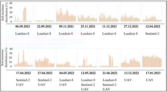
Figure 5.
Overview of the datasets used for each data collection and the corresponding soil moisture content distribution.
UAV Flight Settings and CoSpectroCam Calibration
The data acquisition process with the CoSpectroCam includes options to acquire DarkObject, WhiteObject and Object measurements of radiance and reflectance. With this IoT system for agriculture, experts can generate real-time reflectance data of objects or plants for feature extraction by integrating high-resolution spatial and spectral features. To calculate the relative reflectance of the samples, it is necessary to measure the reflectance of a standard white screen. Therefore, the CoSpectroCam was calibrated with the Spectralon White Diffuse Reflectance Standard prior to data acquisition. The reflectance of the sample was measured using the following equation [34]:
Here, and are the reflectance of the sample and Spectralon, respectively, and and are the radiance of the sample and Spectralon, respectively.
After calibration, the CoSpectroCam was mounted on the UAV. Data acquisition was synchronized with the satellite overflights of the study area and automatic flight operations were performed using Drone Harmony software (version 2.3.0, Drone Harmony Company, Zurich, Switzerland). Data acquisitions were performed on clear, sunny days between 9:00 and 12:00 local time to reduce atmospheric impacts. The UAV flew at a height of 50 m and a speed of 3 m/s. With a vertical and horizontal overlap of 70%, the output maps achieved a spatial resolution of 0.04 m. The entire 100-hectare field was surveyed in five separate UAV missions, with each mission covering around 20 hectares.
Preprocessing UAV Hyperspectral Data
Preprocessing of hyperspectral data is essential to obtain accurate measurements and improve the reliability of subsequent modeling [35]. Spectrometers usually consist of photoelectric conversion, transmission and processing systems, each of which causes a different degree of noise. This noise can distort the actual spectral information of the samples, so it is crucial to identify and eliminate it to ensure the accuracy of the dataset [36]. The CoSpectroCam data are stored as images and spectral tables, both linked by a common timestamp as a reference. For this study, bands with a signal-to-noise ratio below 100 were excluded from the analysis. As a result, wavelengths ranging from 420 nm to 850 nm were utilized. In addition, the spectra were smoothed using the Savitzky–Golay filter, with a window size of 25 and a polynomial degree of 2 (corresponding to 4.2 nm on each side).
Generation of DEM and Orthomosaic Maps
In this study, the RGB images captured by the UAV were processed using Agisoft Metashape Pro software (version 2.0.0, Agisoft Company, St. Petersburg, Russia) to create the orthomosaic map and digital elevation model (DEM) for the study area on each observation day. To ensure accurate georeferencing of the output maps, 10 strategically distributed fixed points were used as ground control points. Figure 6 shows the orthomosaic and DEM maps of the area for 22 September 2021.
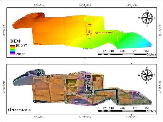
Figure 6.
Orthomosaic and digital elevation model (DEM) maps of the study area, generated from UAV-captured RGB images on 22 September 2021.
2.2.5. Soil Moisture Modeling
The relationship between SMC and the land surface spectrum is very complex, making it difficult for classical regression methods to accurately predict this relationship [37]. However, machine-learning algorithms excel at capturing complex patterns such as nonlinearity and heteroscedasticity [20]. In this study, five machine-learning algorithms, ANN, ELM, PLSR, SVR and GPR, were used for SMC estimation.
ANN is a machine-learning model inspired by the structure and functionality of the human nervous system. It is widely known for its effectiveness in SMC estimation as it is able to model nonlinear relationships within the data [38].
ELM is a machine-learning algorithm developed for Single-Hidden-Layer Feedforward Neural Networks (SLFNs) and was first introduced by Huang et al. [39]. Compared to conventional learning algorithms for feedforward neural networks with a single hidden layer, ELM offers much faster training speed, better generalization capabilities and requires less configuration effort [39].
PLSR was popularized in chemistry by Geladi et al. [40] for the quantitative analysis of spectral reflectance distributions. Since then, it has become a widely used modeling method for visible and infrared spectra analysis [41]. One of the primary benefits of PLSR lies in its proficiency to manage challenging datasets, such as those with missing or noisy data and situations in which there are fewer samples than predictor variables [41,42].
SVR is an analytical method for investigating the relationship between one or more predictor variables and a continuous (real-valued) dependent variable. It is based on the support vector machine model but is tailored to regression tasks. SVR is very effective for modeling soil surface features such as SMC using remote-sensing data [38].
GPR is a data-driven modeling approach based on statistical principles and Bayesian theory. It relies on the Gaussian process for modeling and predicting continuous data. GPR has strong generalization capabilities, which makes it very suitable for a variety of challenging modeling tasks [43].
In this study, the calibration and validation of the machine-learning algorithms were performed using the ARTMO package [44] in MATLAB R2023a. The models were trained using ground truth SMC data as the target variable, and the corresponding pixel values from the aerosol, blue, green, red, NIR, SWIR-1, SWIR-2, TIR-1 and TIR-2 bands from Landsat-8/9, aerosol, blue, green, red, Red Edge 1, Red Edge 2, Red Edge 3, NIR, Red Edge 4, SWIR-1 and SWIR-2 bands from Sentinel-2 as well as hyperspectral data from UAV (wavelengths from 420 to 850 nm) as input variables. A 10-fold cross-validation approach was used to ensure robust validation of the models.
2.2.6. Validation
The mean absolute error (MAE), coefficient of determination (R2) and root mean square error (RMSE) were calculated using the following formulas to assess the effectiveness of the SMC estimation models.
Here, and stand for the observed and predicted SMC, respectively. is the mean value of the observed SMC, n denotes the number of soil samples and m refers to the number of variables.
3. Results and Discussion
3.1. Effects of Soil Moisture Contents on the Spectral Reflectance of the Datasets
The results of the soil analyses in the region showed that the soil texture was relatively uniform in all samples collected, with silty loam being the predominant texture in the study area. In addition, the electrical conductivity, pH and color of the soil samples were relatively uniform (Table S1). Therefore, it was assumed in this study that the basic soil properties of the region were uniform and that only land cover and SMC had an influence on the variances of the soil spectral response.
Figure 7 shows the spectral reflectance captured by UAV, Landsat-8/9 and Sentinel-2 for four pixels representing different levels of SMC and green vegetation measured during the campaigns on 12 May 2022 and 21 June 2022. Comparing Figure 7a and Figure 7b, which show the spectra for bare soil with SMC of 1.41% and 21.5%, respectively, it is clear that pixels with a higher SMC show a decrease in reflectance across the entire spectrum, especially in the UAV data. This decrease is mainly due to changes in the real refractive index of the soil particles. As the SMC increases, the soil becomes darker, absorbing more light and reflecting less. These findings are consistent with the results of Mirzaei et al. [45].
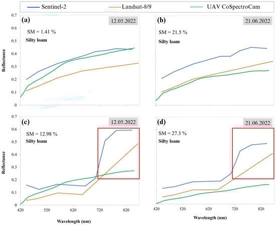
Figure 7.
Spectral reflectance of Landsat-8/9, Sentinel-2 and UAV for (a) dry and bare soil pixels, (b) wet and bare soil pixels, (c) dry and vegetation-covered pixels and (d) wet and vegetation-covered pixels.
Figure 7c and Figure 7d show the spectra for pixels covered with vegetation with an SMC of 12.98% and 27.3%, respectively. However, it should be noted that the UAV data in these figures were derived from soil reflectance and not vegetation, as the field of view (FOV) of the CoSpectroCam mounted on the UAV only captures a rectangular section superimposed on the RGB image (Figure 3). However, the data from Sentinel-2 and Landsat-8/9 correspond to larger pixels, including vegetation and soil surfaces. Therefore, their spectra represent mixed vegetation–soil signals. In Figure 7c, where plant water content is low, the reflectance in the visible range of both the Sentinel-2 and Landsat-8/9 sensors is low due to light absorption by chlorophyll. In the near-infrared (NIR) range, however, a clear increase in reflectance can be observed (red rectangle), which is due to the cell structure of the leaf. This pattern can also be observed in vegetation with high water content (Figure 7d), although the NIR reflectance decreases slightly under wetter conditions.
3.2. Soil Moisture Content Estimation
Figure 8 shows the relationship between the observed SMC and the SMC predicted by different algorithms, with the color of the points representing the NDVI values. The Sentinel-2 data had a relatively low potential for estimating SMC, as shown by the accuracy of the models in estimating SMC, which ranged from 0.42 to 0.46. This finding contradicts the results of Liu et al. [22]. The absence of a thermal band on Sentinel-2 is likely responsible for the reduced accuracy in SMC estimation. Nevertheless, ELM outperformed the other models in estimating SMC with an R2 of 0.46. The PLSR and GPR models ranked second and third with an R2 of 0.45, and the SVR model performed the worst with an R2 of 0.42.
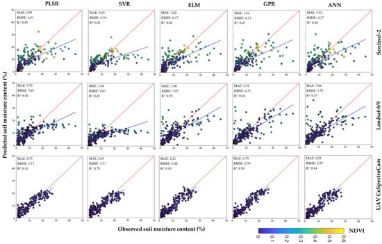
Figure 8.
Comparison of observed versus predicted soil moisture content using PLSR, SVR, ELM, GPR and ANN algorithms with Sentinel-2 (up), Landsat-8/9 (middle) and UAV (down) data.
The SMC estimation accuracy of the different models for the Landsat-8/9 data varied between 0.45 and 0.64, indicating that the data have a comparatively high potential for SMC estimation [23,46,47]. The GPR model outperformed the other models and achieved an R2 of 0.64. The ELM and ANN models ranked second and third with R2 values of 0.59 and 0.55, respectively. Of all the models, the SVR model showed the weakest performance in estimating SMC using Landsat 8/9 data, with an R2 of 0.45.
For the UAV hyperspectral data, the GPR model delivered the best performance of all models with an R2 of 0.89. The ELM and ANN models ranked second and third with R2 values of 0.85 and 0.84, respectively. The SVR model showed the weakest performance in estimating SMC using UAV hyperspectral data with an R2 of 0.78.
A comparison with the results of Shokati et al. [17] showed that their random forest model performed relatively better than our models when using Sentinel-2 and Landsat-8/9 data; however, our GPR model outperformed their results when applied to UAV hyperspectral data. Furthermore, our UAV-based results surpassed those reported by Shokati et al. [18] and Cheng et al. [29], despite their use of different UAV-mounted sensors.
A comparison of the observed SMC and the SMC predicted by different models using Sentinel-2, Landsat-8/9 and UAV data (Figure 8) showed that all models generally overestimated the SMC in areas with less than 8% SMC. However, in regions with an SMC of more than 8%, the models generally underestimated the SMC [18]. In Sentinel-2 data, the ELM model exhibited less overestimation and underestimation than the other models. Conversely, the GPR model demonstrated the lowest levels of overestimation and underestimation for the Landsat-8/9 and UAV data. The SVR model showed the highest values for over- and underestimation for all datasets. The reason for this over- and underestimation can be attributed to the spatial resolution of the datasets, which causes a lack of uniformity and purity of the pixels [48]. In other words, a single pixel can represent a heterogeneous area containing diverse land-cover types even though it has been assigned a uniform value. However, it should be noted that no quantitative purity index or spectral unmixing analysis was performed in this study to assess the degree of pixel heterogeneity. The overestimation and underestimation of SMC with UAV data was lower than that of Sentinel-2 and Landsat-8/9. The reason for this is the higher spatial and spectral resolution of CoSpectroCam mounted on the UAV compared to the two satellites. The higher spectral resolution of CoSpectroCam allows a more detailed insight into the spectral behavior of the soil, and the higher spatial resolution leads to greater pixel uniformity. Other factors that affect the higher accuracy of UAV data are the preprocessing of the data, such as the removal of noise and the smoothing of the data. These advantages highlight the potential of UAV-based hyperspectral imaging for precision agriculture applications, especially in optimizing irrigation strategies through accurate SMC monitoring.
Figure 9 shows the Taylor diagram illustrating the performance of the models developed with different datasets. The analysis of SMC estimation revealed that regardless of the model type, the hyperspectral data from UAV outperformed the multispectral data from Sentinel-2 and Landsat-8/9 in estimating SMC. In addition, Landsat-8/9 data showed a higher accuracy than Sentinel-2 data for all models. This discrepancy is partly due to the absence of a thermal band in the Sentinel-2 sensors.
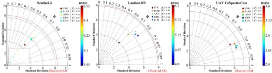
Figure 9.
Taylor diagram illustrating the performance of models developed using Sentinel-2, Landsat-8/9 and UAV data.
A comparison of the different models revealed that the GPR model performed best when using UAV and Landsat-8/9 data, while the ELM model performed best with Sentinel-2 data. Conversely, the SVR model consistently delivered the weakest performance across all datasets. This lower performance of SVR can be attributed to its sensitivity to high-dimensional input features, such as those in hyperspectral data. In addition, SVR may be less effective on small datasets, as the performance of the model depends heavily on optimal kernel selection and parameter tuning. These results are consistent with the conclusions of Singh and Gaurav [49].
Figure 10 shows the SMC maps predicted by different models using Sentinel-2 and Landsat-8/9 data for 12 May 2022. The results showed that regardless of the model type, both datasets had a similar pattern in SMC estimation. Higher SMC was observed in vegetated areas compared to unvegetated land, which is likely due to better moisture retention in vegetated regions. The higher spatial resolution of the Sentinel-2 imagery allowed the predicted SMC maps to show the regional SMC distribution in more detail than the maps produced with Landsat-8/9 data. In addition, the results showed that the SVR model consistently predicted lower SMC values than other models, regardless of the dataset used.
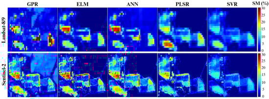
Figure 10.
Soil moisture content maps derived from Landsat-8/9 and Sentinel-2 data using different models for 12 May 2022.
3.3. Sensitivity of the UAV Hyperspectral Bands
The GPR model demonstrated a superior performance in SMC modeling using UAV hyperspectral data. As a Bayesian framework-based approach, the GPR model contains a sigma parameter that indicates the importance of individual spectral bands or components. Lower sigma values indicate greater significance as they correspond to bands that make a greater contribution to the predictive power of the model.
Figure 11 illustrates the sigma values for the wavelengths captured by the CoSpectroCam sensor. The analysis revealed that the wavelengths with the highest sensitivity for SMC were mainly concentrated in the blue and red-edge regions of the spectrum. This observation is consistent with the results of Ge et al. [28] who also found these regions to be particularly informative for SMC estimation. Their study attributed this sensitivity to the interaction between SMC and vegetation water status, which affects chlorophyll-related reflectance characteristics. In our study, the wavelength at 777 nm exhibited the smallest sigma value, indicating its exceptional sensitivity and critical role in the accurate estimation of SMC. This finding underscores the potential of utilizing these spectral regions for improved SMC prediction and highlights the importance of the red-edge and blue bands in hyperspectral analysis for environmental applications.
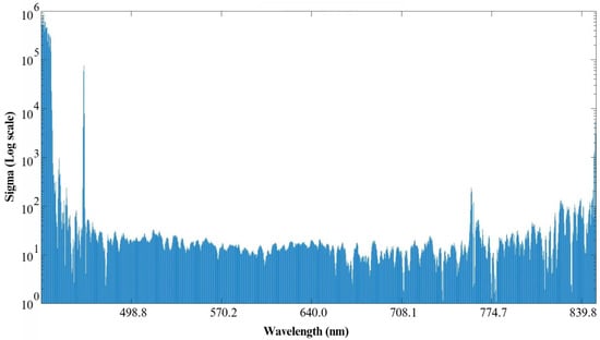
Figure 11.
Sigma values for different wavelengths of UAV hyperspectral data.
3.4. Effects of Land Cover on Soil Moisture Content Retrieval Accuracy
As shown in Figure 8, the SMC values were closely linked to the NDVI index. However, the NDVI values differed from dataset to dataset due to different data collection dates, resulting in differences in vegetation cover. In addition, the CoSpectroCam sensor’s focus on the central areas of the images produced pure spectra, resulting in lower NDVI values. Since vegetation and SMC are directly related, these variations in vegetation can affect the accuracy of SMC retrieval. To investigate this, the study area was categorized into three land-cover types: bare soil, cropland and grassland. In each data collection session, we systematically collected an equal number of SMC samples from each land-cover type to ensure balanced representation (15 samples per type per day). The performance of the models and datasets was then analyzed for each land-cover type. The results presented in Figure 12 showed that the models had a higher accuracy on bare soil than on cropland and grassland. These results are consistent with those of Petropoulos et al. [8] and Liu et al. [22].
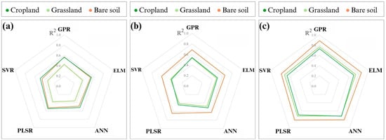
Figure 12.
Performance of different models in predicting soil moisture content over different land-cover types using (a) Sentinel-2, (b) Landsat-8/9 and (c) UAV hyperspectral data.
Sentinel-2 data showed a strong performance in SMC estimation in cropland environments [22,50,51]. This performance can be attributed in part to the presence of four red-edge bands in Sentinel-2 imagery, which are particularly valuable for vegetation studies [51]. Since the water content of vegetation is indirectly influenced by the SMC [52,53], these red-edge bands increase the potential of Sentinel-2 data for accurate estimation of SMC in croplands. Conversely, the Sentinel-2 data showed a lower performance in estimating SMC over grassland, which is probably related to the heterogeneity of these areas. Across all land-cover types, the GPR model proved to be the most effective with an R2 of 0.57 for bare soil, 0.56 for cropland and 0.43 for grassland. In contrast, the SVR model consistently showed the lowest accuracy in SMC estimation across all land-cover classes.
Models developed with Landsat-8/9 data performed better in estimating SMC over bare soil than over cropland and grassland. This better performance can be attributed to the uniformity of bare soil and the availability of thermal bands in the Landsat-8/9 satellites. However, as vegetation cover increased, the accuracy of SMC estimation with Landsat-8/9 data decreased, resulting in a lower performance over cropland and grassland [23]. Of all the models, the GPR model consistently showed the highest accuracy across different land covers. For bare soil, the GPR model achieved an R2 of 0.69, but its performance decreased for cropland and grassland, with R2 values of 0.54 and 0.53, respectively [29]. On bare soil and cropland, the SVR model showed the lowest accuracy with R2 values of 0.60 and 0.41, respectively. On grassland, on the other hand, the PLSR model showed the worst performance with an R2 of 0.41.
Similar to the Sentinel-2 and Landsat-8/9 data, the UAV hyperspectral data showed the highest performance in SMC estimation over bare soil in all models. Remarkably, the UAV hyperspectral data also provided better results for grassland than for cropland, which could be due to the delayed response of crops to changes in SMC. In all land-cover types, the GPR model with UAV data performed consistently better than the other models, achieving R2 values of 0.89 for bare soil, 0.73 for cropland and 0.77 for grassland. The ELM model came second in terms of performance. Conversely, the SVR model showed the lowest accuracy in SMC estimation across all land-cover types, with R2 values of 0.78 for bare soil, 0.66 for cropland and 0.71 for grassland.
A comparison of the performance of different datasets revealed that models developed with UAV hyperspectral data achieved higher accuracy in SMC estimation in all land-cover classes than models based on Landsat-8/9 and Sentinel-2 data. This better performance can be attributed to the high spatial and spectral resolution of the CoSpectroCam sensor mounted on the UAV. A comparison between Sentinel-2 and Landsat-8/9 data also showed that Sentinel-2 has a higher accuracy in SMC estimation for cropland [21]. This advantage is likely due to the presence of four red-edge bands in Sentinel-2. In addition, the higher reflectance values of the Landsat-8/9 bands compared to Sentinel-2 may excessively reduce the contribution of vegetation distribution, which decreases the accuracy of SMC estimation for cropland compared to Sentinel-2 [21]. However, for bare soil and grassland, Landsat-8/9 data showed a higher accuracy in SMC estimation compared to Sentinel-2 data. To assess whether the differences in model performance between land covers are significant, tests such as ANOVA or t-tests are recommended. This was not performed in this study but is suggested for future work.
4. Conclusions
In this study, UAV-based spectroscopy, synchronized with satellite overflights, was used to improve SMC estimation with different machine-learning algorithms and to assess the impact of land cover. The results showed that UAV-based aerial spectroscopy significantly improved the accuracy of SMC estimation compared to satellite-based data, highlighting its potential for precision agriculture. Among the machine-learning algorithms, GPR performed best on UAV and Landsat-8/9 data, while ELM performed best on Sentinel-2 data. However, our experiments were conducted in a limited area and under site-specific soil and vegetation conditions. Scaling UAV deployments to regional extents remains a challenge due to flight duration, coverage and data processing limitations. To overcome these limitations, future research should integrate machine learning with physical-based models such as the multilayer radiative transfer model of soil reflectance (MARMIT), employ transfer learning to adapt pre-trained models to new environments and investigate swarm UAV systems or optimized flight planning for large-scale SMC monitoring. These efforts will be critical to advancing scalable, highly accurate SMC estimates for precision agriculture and more effective management of plant health and water resources.
Supplementary Materials
The following supporting information can be downloaded at: https://www.mdpi.com/article/10.3390/w17111715/s1, Figure S1: Overview of soil properties in the region: texture, color, pH, and electrical conductivity (EC); Table S1: Summary statistics of soil properties.
Author Contributions
Conceptualization: H.S. and Z.M.-D.; Methodology: H.S., S.M. and Z.M.-D.; Formal analysis and investigation: H.S.; Writing—original draft preparation: H.S.; Writing—review and editing: M.M., A.N., S.M., K.N., R.T.-M. and T.S.; Visualization: H.S., R.A. and L.H.; Software: H.S., S.M. and P.K.; Supervision: M.M., A.N. and T.S. All authors have read and agreed to the published version of the manuscript.
Funding
This research received no external funding.
Data Availability Statement
The datasets generated during and analyzed during the current study are available from the corresponding author on reasonable request.
Conflicts of Interest
The authors declare no conflicts of interest.
References
- Ahmad, S.; Kalra, A.; Stephen, H. Estimating Soil Moisture Using Remote Sensing Data: A Machine Learning Approach. Adv. Water Resour. 2010, 33, 69–80. [Google Scholar] [CrossRef]
- Grayson, R.B.; Western, A.W.; Chiew, F.H.S.; Blöschl, G. Preferred States in Spatial Soil Moisture Patterns: Local and Nonlocal Controls. Water Resour. Res. 1997, 33, 2897–2908. [Google Scholar] [CrossRef]
- Hino, M.; Odaka, Y.; Nadaoka, K.; Sato, A. Effect of Initial Soil Moisture Content on the Vertical Infiltration Process—A Guide to the Problem of Runoff-Ratio and Loss. J. Hydrol. 1988, 102, 267–284. [Google Scholar] [CrossRef]
- Western, A.W.; Grayson, R.B.; Blöschl, G. Scaling of Soil Moisture: A Hydrologic Perspective. Annu. Rev. Earth Planet. Sci. 2002, 30, 149–180. [Google Scholar] [CrossRef]
- Carrão, H.; Russo, S.; Sepulcre-Canto, G.; Barbosa, P. An Empirical Standardized Soil Moisture Index for Agricultural Drought Assessment from Remotely Sensed Data. Int. J. Appl. Earth Obs. Geoinf. 2016, 48, 74–84. [Google Scholar] [CrossRef]
- Holzman, M.E.; Rivas, R.; Piccolo, M.C. Estimating Soil Moisture and the Relationship with Crop Yield Using Surface Temperature and Vegetation Index. Int. J. Appl. Earth Obs. Geoinf. 2014, 28, 181–192. [Google Scholar] [CrossRef]
- Korres, W.; Reichenau, T.G.; Fiener, P.; Koyama, C.N.; Bogena, H.R.; Cornelissen, T.; Baatz, R.; Herbst, M.; Diekkrüger, B.; Vereecken, H.; et al. Spatio-Temporal Soil Moisture Patterns—A Meta-Analysis Using Plot to Catchment Scale Data. J. Hydrol. 2015, 520, 326–341. [Google Scholar] [CrossRef]
- Petropoulos, G.P.; Ireland, G.; Barrett, B. Surface Soil Moisture Retrievals from Remote Sensing: Current Status, Products & Future Trends. Phys. Chem. Earth Parts A/B/C 2015, 83–84, 36–56. [Google Scholar] [CrossRef]
- Wang, L.; Qu, J.J. Satellite Remote Sensing Applications for Surface Soil Moisture Monitoring: A Review. Front. Earth Sci. China 2009, 3, 237–247. [Google Scholar] [CrossRef]
- Lu, F.; Sun, Y.; Hou, F. Using UAV Visible Images to Estimate the Soil Moisture of Steppe. Water 2020, 12, 2334. [Google Scholar] [CrossRef]
- Zhang, D.; Zhou, G. Estimation of Soil Moisture from Optical and Thermal Remote Sensing: A Review. Sensors 2016, 16, 1308. [Google Scholar] [CrossRef]
- Ångström, A. The Albedo of Various Surfaces of Ground. Geogr. Ann. 1925, 7, 323–342. [Google Scholar]
- Curcio, J.A.; Petty, C.C. The Near Infrared Absorption Spectrum of Liquid Water. J. Opt. Soc. Am. JOSA 1951, 41, 302–304. [Google Scholar] [CrossRef]
- Lendzioch, T.; Langhammer, J.; Vlček, L.; Minařík, R. Mapping the Groundwater Level and Soil Moisture of a Montane Peat Bog Using UAV Monitoring and Machine Learning. Remote Sens. 2021, 13, 907. [Google Scholar] [CrossRef]
- Adab, H.; Morbidelli, R.; Saltalippi, C.; Moradian, M.; Ghalhari, G.A.F. Machine Learning to Estimate Surface Soil Moisture from Remote Sensing Data. Water 2020, 12, 3223. [Google Scholar] [CrossRef]
- Nguyen, T.T.; Ngo, H.H.; Guo, W.; Chang, S.W.; Nguyen, D.D.; Nguyen, C.T.; Zhang, J.; Liang, S.; Bui, X.T.; Hoang, N.B. A Low-Cost Approach for Soil Moisture Prediction Using Multi-Sensor Data and Machine Learning Algorithm. Sci. Total Environ. 2022, 833, 155066. [Google Scholar] [CrossRef] [PubMed]
- Shokati, H.; Mashal, M.; Noroozi, A.; Abkar, A.A.; Mirzaei, S.; Mohammadi-Doqozloo, Z.; Taghizadeh-Mehrjardi, R.; Khosravani, P.; Nabiollahi, K.; Scholten, T. Random Forest-Based Soil Moisture Estimation Using Sentinel-2, Landsat-8/9, and UAV-Based Hyperspectral Data. Remote Sens. 2024, 16, 1962. [Google Scholar] [CrossRef]
- Shokati, H.; Mashal, M.; Noroozi, A.; Mirzaei, S.; Mohammadi-Doqozloo, Z. Assessing Soil Moisture Levels Using Visible UAV Imagery and Machine Learning Models. Remote Sens. Appl. Soc. Environ. 2023, 32, 101076. [Google Scholar] [CrossRef]
- Rabiei, S.; Jalilvand, E.; Tajrishy, M. A Method to Estimate Surface Soil Moisture and Map the Irrigated Cropland Area Using Sentinel-1 and Sentinel-2 Data. Sustainability 2021, 13, 11355. [Google Scholar] [CrossRef]
- Liu, Q.; Wu, Z.; Cui, N.; Jin, X.; Zhu, S.; Jiang, S.; Zhao, L.; Gong, D. Estimation of Soil Moisture Using Multi-Source Remote Sensing and Machine Learning Algorithms in Farming Land of Northern China. Remote Sens. 2023, 15, 4214. [Google Scholar] [CrossRef]
- Wang, Q.; Li, J.; Jin, T.; Chang, X.; Zhu, Y.; Li, Y.; Sun, J.; Li, D. Comparative Analysis of Landsat-8, Sentinel-2, and GF-1 Data for Retrieving Soil Moisture over Wheat Farmlands. Remote Sens. 2020, 12, 2708. [Google Scholar] [CrossRef]
- Liu, Y.; Qian, J.; Yue, H. Comprehensive Evaluation of Sentinel-2 Red Edge and Shortwave-Infrared Bands to Estimate Soil Moisture. IEEE J. Sel. Top. Appl. Earth Obs. Remote Sens. 2021, 14, 7448–7465. [Google Scholar] [CrossRef]
- Mobasheri, M.R.; Amani, M. Soil Moisture Content Assessment Based on Landsat 8 Red, near-Infrared, and Thermal Channels. JARS 2016, 10, 026011. [Google Scholar] [CrossRef]
- Ge, X.; Ding, J.; Jin, X.; Wang, J.; Chen, X.; Li, X.; Liu, J.; Xie, B. Estimating Agricultural Soil Moisture Content through UAV-Based Hyperspectral Images in the Arid Region. Remote Sens. 2021, 13, 1562. [Google Scholar] [CrossRef]
- Aboutalebi, M.; Allen, L.N.; Torres-Rua, A.F.; McKee, M.; Coopmans, C. Estimation of Soil Moisture at Different Soil Levels Using Machine Learning Techniques and Unmanned Aerial Vehicle (UAV) Multispectral Imagery. In Proceedings of the Autonomous Air and Ground Sensing Systems for Agricultural Optimization and Phenotyping IV, Baltimore, MD, USA, 15–16 May 2019; Volume 11008, pp. 216–226. [Google Scholar]
- de Lima, R.S.; Li, K.-Y.; Vain, A.; Lang, M.; Bergamo, T.F.; Kokamägi, K.; Burnside, N.G.; Ward, R.D.; Sepp, K. The Potential of Optical UAS Data for Predicting Surface Soil Moisture in a Peatland across Time and Sites. Remote Sens. 2022, 14, 2334. [Google Scholar] [CrossRef]
- Hassan-Esfahani, L.; Torres-Rua, A.; Jensen, A.; McKee, M. Assessment of Surface Soil Moisture Using High-Resolution Multi-Spectral Imagery and Artificial Neural Networks. Remote Sens. 2015, 7, 2627–2646. [Google Scholar] [CrossRef]
- Ge, X.; Wang, J.; Ding, J.; Cao, X.; Zhang, Z.; Liu, J.; Li, X. Combining UAV-Based Hyperspectral Imagery and Machine Learning Algorithms for Soil Moisture Content Monitoring. PeerJ 2019, 7, e6926. [Google Scholar] [CrossRef]
- Cheng, M.; Jiao, X.; Liu, Y.; Shao, M.; Yu, X.; Bai, Y.; Wang, Z.; Wang, S.; Tuohuti, N.; Liu, S.; et al. Estimation of Soil Moisture Content under High Maize Canopy Coverage from UAV Multimodal Data and Machine Learning. Agric. Water Manag. 2022, 264, 107530. [Google Scholar] [CrossRef]
- Luo, W.; Xu, X.; Liu, W.; Liu, M.; Li, Z.; Peng, T.; Xu, C.; Zhang, Y.; Zhang, R. UAV Based Soil Moisture Remote Sensing in a Karst Mountainous Catchment. CATENA 2019, 174, 478–489. [Google Scholar] [CrossRef]
- Hummel, J.W.; Sudduth, K.A.; Hollinger, S.E. Soil Moisture and Organic Matter Prediction of Surface and Subsurface Soils Using an NIR Soil Sensor. Comput. Electron. Agric. 2001, 32, 149–165. [Google Scholar] [CrossRef]
- Roy, S.K.; Shibusawa, S.; Okayama, T. Textural Analysis of Soil Images to Quantify and Characterize the Spatial Variation of Soil Properties Using a Real-Time Soil Sensor. Precis. Agric. 2006, 7, 419–436. [Google Scholar] [CrossRef]
- Bouyoucos, G.J. Hydrometer Method Improved for Making Particle Size Analyses of Soils1. Agron. J. 1962, 54, 464–465. [Google Scholar] [CrossRef]
- Oltra-Carrió, R.; Baup, F.; Fabre, S.; Fieuzal, R.; Briottet, X. Improvement of Soil Moisture Retrieval from Hyperspectral VNIR-SWIR Data Using Clay Content Information: From Laboratory to Field Experiments. Remote Sens. 2015, 7, 3184–3205. [Google Scholar] [CrossRef]
- Li, S.; Shi, Z.; Chen, S.; Ji, W.; Zhou, L.; Yu, W.; Webster, R. In Situ Measurements of Organic Carbon in Soil Profiles Using Vis-NIR Spectroscopy on the Qinghai–Tibet Plateau. Environ. Sci. Technol. 2015, 49, 4980–4987. [Google Scholar] [CrossRef] [PubMed]
- Jin, X.; Du, J.; Liu, H.; Wang, Z.; Song, K. Remote Estimation of Soil Organic Matter Content in the Sanjiang Plain, Northest China: The Optimal Band Algorithm versus the GRA-ANN Model. Agric. For. Meteorol. 2016, 218–219, 250–260. [Google Scholar] [CrossRef]
- Koley, S.; Jeganathan, C. Estimation and Evaluation of High Spatial Resolution Surface Soil Moisture Using Multi-Sensor Multi-Resolution Approach. Geoderma 2020, 378, 114618. [Google Scholar] [CrossRef]
- Ali, I.; Greifeneder, F.; Stamenkovic, J.; Neumann, M.; Notarnicola, C. Review of Machine Learning Approaches for Biomass and Soil Moisture Retrievals from Remote Sensing Data. Remote Sens. 2015, 7, 16398–16421. [Google Scholar] [CrossRef]
- Huang, G.-B.; Zhu, Q.-Y.; Siew, C.-K. Extreme Learning Machine: A New Learning Scheme of Feedforward Neural Networks. In Proceedings of the 2004 IEEE International Joint Conference on Neural Networks (IEEE Cat. No.04CH37541), Budapest, Hungary, 25–29 July 2004; Volume 2, pp. 985–990. [Google Scholar]
- Geladi, P.; Kowalski, B.R. Partial Least-Squares Regression: A Tutorial. Anal. Chim. Acta 1986, 185, 1–17. [Google Scholar] [CrossRef]
- Rossel, R.A.V.; Behrens, T. Using Data Mining to Model and Interpret Soil Diffuse Reflectance Spectra. Geoderma 2010, 158, 46–54. [Google Scholar] [CrossRef]
- Elkharrouba, E.; Sekertekin, A.; Fathi, J.; Tounsi, Y.; Bioud, H.; Nassim, A. Surface Soil Moisture Estimation Using Dual-Polarimetric Stokes Parameters and Backscattering Coefficient. Remote Sens. Appl. Soc. Environ. 2022, 26, 100737. [Google Scholar] [CrossRef]
- Liu, M.; Huang, C.; Wang, L.; Zhang, Y.; Luo, X. Short-Term Soil Moisture Forecasting via Gaussian Process Regression with Sample Selection. Water 2020, 12, 3085. [Google Scholar] [CrossRef]
- Caicedo, J.P.R.; Verrelst, J.; Muñoz-Marí, J.; Moreno, J.; Camps-Valls, G. Toward a Semiautomatic Machine Learning Retrieval of Biophysical Parameters. IEEE J. Sel. Top. Appl. Earth Obs. Remote Sens. 2014, 7, 1249–1259. [Google Scholar] [CrossRef]
- Mirzaei, S.; Darvishi Boloorani, A.; Bahrami, H.A.; Alavipanah, S.K.; Mousivand, A.; Mouazen, A.M. Minimising the Effect of Moisture on Soil Property Prediction Accuracy Using External Parameter Orthogonalization. Soil Tillage Res. 2022, 215, 105225. [Google Scholar] [CrossRef]
- Hezarian, F.; Khalilimoghadam, B.; Zoratipour, A.; Nejad, M.F.; Yusefi, A. Assessment of the Capability of Satellite Images in Determining the Topsoil Moisture Content in the Dust Hotspot of Southeastern Ahvaz in Iran. Eurasian Soil Sci. 2022, 55, 1576–1590. [Google Scholar] [CrossRef]
- Zhang, Y.; Liang, S.; Zhu, Z.; Ma, H.; He, T. Soil Moisture Content Retrieval from Landsat 8 Data Using Ensemble Learning. ISPRS J. Photogramm. Remote Sens. 2022, 185, 32–47. [Google Scholar] [CrossRef]
- Foody, G.M.; Cox, D.P. Sub-Pixel Land Cover Composition Estimation Using a Linear Mixture Model and Fuzzy Membership Functions. Int. J. Remote Sens. 1994, 15, 619–631. [Google Scholar] [CrossRef]
- Singh, A.; Gaurav, K. Deep Learning and Data Fusion to Estimate Surface Soil Moisture from Multi-Sensor Satellite Images. Sci. Rep. 2023, 13, 2251. [Google Scholar] [CrossRef] [PubMed]
- Ambrosone, M.; Matese, A.; Di Gennaro, S.F.; Gioli, B.; Tudoroiu, M.; Genesio, L.; Miglietta, F.; Baronti, S.; Maienza, A.; Ungaro, F.; et al. Retrieving Soil Moisture in Rainfed and Irrigated Fields Using Sentinel-2 Observations and a Modified OPTRAM Approach. Int. J. Appl. Earth Obs. Geoinf. 2020, 89, 102113. [Google Scholar] [CrossRef]
- Hegazi, E.H.; Samak, A.A.; Yang, L.; Huang, R.; Huang, J. Prediction of Soil Moisture Content from Sentinel-2 Images Using Convolutional Neural Network (CNN). Agronomy 2023, 13, 656. [Google Scholar] [CrossRef]
- Jackson, T.J.; Chen, D.; Cosh, M.; Li, F.; Anderson, M.; Walthall, C.; Doriaswamy, P.; Hunt, E.R. Vegetation Water Content Mapping Using Landsat Data Derived Normalized Difference Water Index for Corn and Soybeans. Remote Sens. Environ. 2004, 92, 475–482. [Google Scholar] [CrossRef]
- Yilmaz, M.T.; Hunt, E.R.; Jackson, T.J. Remote Sensing of Vegetation Water Content from Equivalent Water Thickness Using Satellite Imagery. Remote Sens. Environ. 2008, 112, 2514–2522. [Google Scholar] [CrossRef]
Disclaimer/Publisher’s Note: The statements, opinions and data contained in all publications are solely those of the individual author(s) and contributor(s) and not of MDPI and/or the editor(s). MDPI and/or the editor(s) disclaim responsibility for any injury to people or property resulting from any ideas, methods, instructions or products referred to in the content. |
© 2025 by the authors. Licensee MDPI, Basel, Switzerland. This article is an open access article distributed under the terms and conditions of the Creative Commons Attribution (CC BY) license (https://creativecommons.org/licenses/by/4.0/).