Soil Moisture Retrieval in North America with Passive Microwave and Auxiliary Data Based on Variable Spatial Optimization

Abstract

Soil moisture content (SMC) is critical in hydrological, agricultural, and meteorological research. There is an urgent need for spatiotemporal information on accurate SMC distribution on a large scale. Passive microwave remote sensing data are among the most commonly used sources for soil moisture retrieval. However, due to the high spatial heterogeneity of SMC and the low spatial resolution of passive microwave data, the SMC condition in the pixel of passive microwave data is rather complex. We propose a method incorporating spatially optimized auxiliary data related to land cover and normalized difference vegetation index (NDVI) to represent the SMC spatial heterogeneity. New variables, “percentages of typical land cover classes” and “average NDVIs corresponding to typical land cover classes”, were introduced. Random forest was adopted to construct an SMC retrieving model. The results of testing samples showed that after “percentages of typical land cover classes” were added into the input parameters, the maximum rise of correlation coefficient (r) was 0.114, and the ultimate decline of unbiased root mean square error (ubRMSE) was 0.0239 cm³cm⁻³. Similarly, substituting NDVI with “average NDVIs corresponding to typical land cover classes” increasesd r by 0.023, and ubRMSE declined by 0.0042 cm³cm⁻³ at most. For the optimal situation, where both groups of new variables were applied, the highest rise of r is 0.127, and the maximum decrease of ubRMSE is 0.0277 cm³cm⁻³.

1. Introduction

The soil moisture content (SMC) refers to the volume of water present in the gaps between surface soil granules. The SMC plays an essential role in climate change investigations and climate prediction. Understanding SMC is crucial for optimizing irrigation practices, enhancing crop productivity, monitoring ecological restoration stages, and mitigating droughts and floods [1,2,3]. For conventional SMC measuring methods, such as time-domain reflectometry [4] and gravimetric technique [5], although they can provide relatively precise SMC values [6], it is challenging to implement SMC monitoring in large areas, and the spatial heterogeneity patterns of land surface SMC are complex to acquire [7,8]. Passive microwave remote sensing uses microwave emission data of the land surface. It detects the difference in emission intensity over the soil, which is highly correlated to the dielectric properties of soil. The direct relationship between SMC and passive microwave measurements guarantees reliable estimations of SMC [9]. In addition, the passive microwave technique can achieve continuous observation over a wide range of areas regardless of sunlight illumination and weather conditions. Recently, great works of SMC retrieval have been accomplished with passive microwave sensors or satellites such as Advanced Microwave Scanning Radiometer 2 (AMSR2), Advanced Microwave Scanning Radiometer-Earth Observing System (AMSR-E), Soil Moisture and Ocean Salinity (SMOS), and Soil Moisture Active Passive (SMAP) [10,11,12].

In the early years, researchers proposed a series of physical or semi-empirical models to formulate microwave radiative transfer [13,14,15,16]. These models allow SMC to be estimated with a guaranteed physical foundation. However, several limitations must be considered; for example, physical models entail much-complicated calculation, which overshadows their application to SMC retrieval on a sizeable scale [17]; similarly, for semi-empirical models, information on vegetation type and surface roughness is conditionally required, which is hard to acquire in the field survey [9,18]. Random forest (RF), one of the standard machine learning models, is an empirical model that can grasp the innate relationship between the input and output data by training and adaptively finding the optimal function to resolve non-linear problems. Instead of several fixed variables, RF models are flexible, manifold, and free from complex physical processes and necessary land surface information [19]. Numerous studies have been conducted on SMC retrieval with RF methods using passive microwave and auxiliary data. Zhang et al. [20] focused on X-band data from the Fengyun Microwave Radiation Imager (MWRI) and investigated the performance of the RF model in SMC retrieval. The results proved the possibility of employing the RF training model to estimate SMC independently and the effect of Fengyun data on ensuring data integrity and increasing data density. Tong et al. [21] compared the results of retrieving temporal dynamics of SMC from 2015 to 2019 using three models (RF, Support Vector Machine, and Ordinary Least Squares) utilizing SMAP data and Moderate-resolution Imaging Spectroradiometer (MODIS) data. The results suggested that the RF model performed better than the other two models and agreed with the ground measurements. Ma et al. [22] utilized SMAP and Advanced Scatterometer (ASCAT) observations to map surface SMC by RF model, and the integration retrievals of surface SMC showed satisfactory performance with enhanced averaged retrieving accuracy and improved temporal resolution.

From the existing literature, it can be found that there is a marked difference in the variables chosen as input parameters, which are crucial for SMC retrieval by RF models. Their suitable selection is necessary because the accuracy of SMC retrieval is subject to the model configuration [23]. Apart from passive microwave brightness temperature, auxiliary data from other sources, e.g., the vegetation condition and land use, are also essential concerning the involvement of relevant geographical factors in microwave radiative transfer [24]. Normalized difference vegetation index (NDVI) and land cover are two suitable variables to represent the features of the vegetation condition and land use and have been utilized by several studies as the input parameters of machine learning models for SMC retrieval [21,25,26] for better description of the relationship between the data. However, in traditional SMC retrieving methods of machine learning, all the data must be rescaled at the resolution of passive microwave data (approximately 10~40 km), and training/testing samples for the model need to be established according to the values in each pixel. Due to the coarse spatial resolution, substantial spatial heterogeneity exists in these pixels, resulting in growing uncertainty in SMC retrievals [27,28]. More specifically, it is typical for a pixel in an image of passive microwave observations to contain various land covers, and using a single value to represent the land cover attribute of the entire pixel area is inappropriate. Similarly, vegetation growth varies considerably within each pixel in an image of passive microwave observations, and details are likely lost if a mere spatially averaged NDVI value is adopted.

This study uses RF and passive microwave data to retrieve SMC. Given the coarse spatial resolution, several “spatially optimized” variables were carried out. These “spatially optimized” variables used a group of values instead of one single value to represent the attribute of auxiliary data in the coarse passive microwave pixels, characterizing the information in greater detail. By comparing statistical metrics of SMC retrieval before and after the involvement of these new variables, the influence of introducing “spatially optimized” variables was checked, and the improvement of SMC retrieving accuracy was discussed. The rest of this paper is organized as follows. In Section 2, the study area and dataset are introduced, the algorithm is specified, the procedure of data preprocessing and establishing sample pools is given, and the combinations of input parameters in the RF algorithm are listed. In Section 3, the SMC retrieval results of different scenarios are given. In Section 4, the analyses and discussion are provided. In Section 5, the conclusions drawn from this study are presented.

2. Materials and Methods

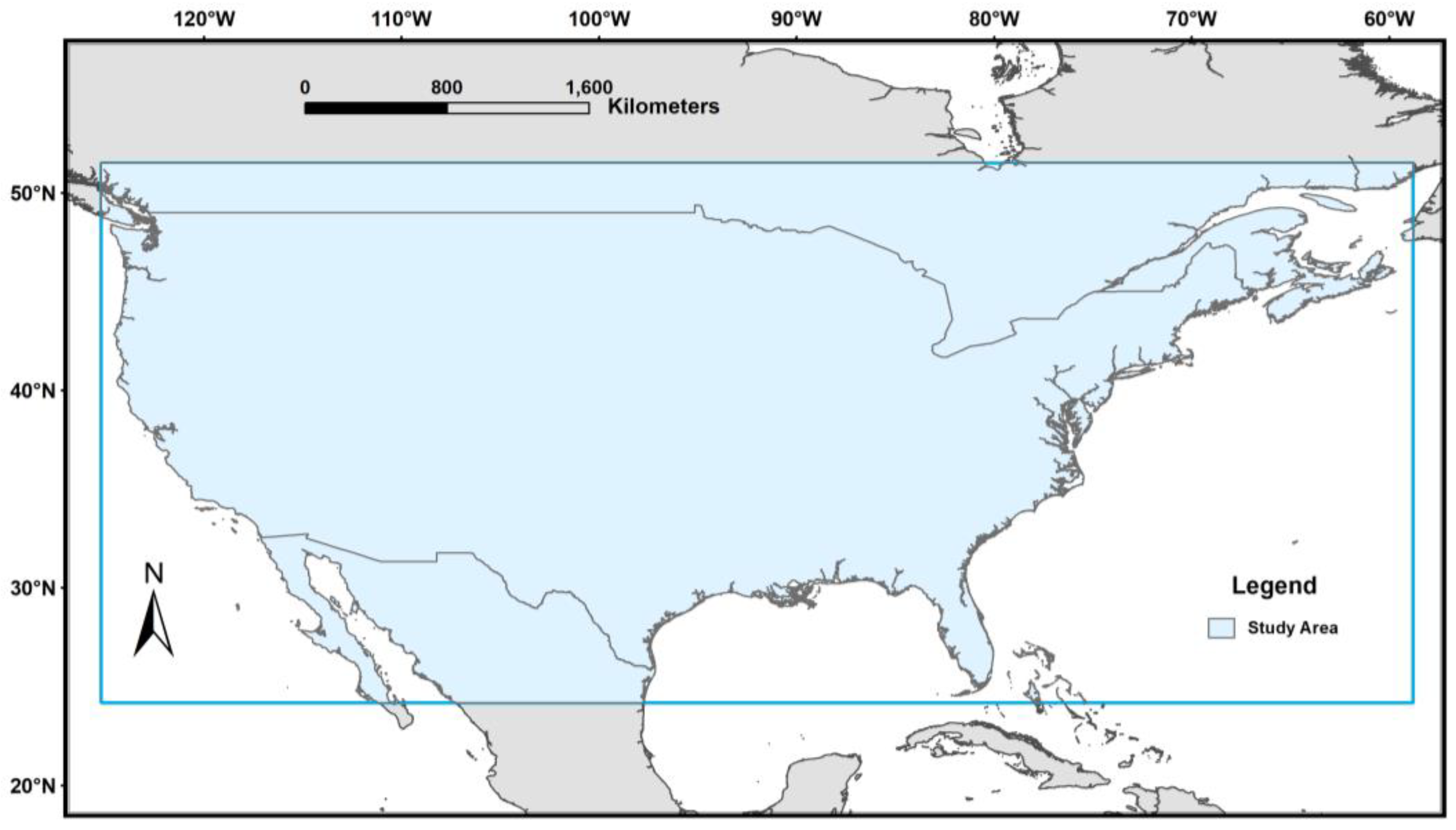
2.1. Study Area

For the case, a rectangular area in North America that includes the contiguous United States, southern Canada, northern Mexico, and the northern Bahamas (Figure 1) was delineated as the study area over the range of 24.2° N~51.5° N latitude and 125.2° W~58.8° W longitude. The study area is characterized by various landforms, with hills in the east, vast plains spread in the middle, and plateaus/mountains dominating the western part. The climate of the study area is mainly temperate and subtropical. The total geographical area of the study area is about 11,970,000 km².

2.2. Data Description

The data used in this study include ERA5-Land modeled data, SMAP brightness temperature data, MODIS data, and Global Land Cover product with Fine Classification System in 30 m (GLC_FCS30) data. Considering data accessibility from various sources, a period between April 2015 and March 2017 was determined for data acquisition. We chose data on each month’s fifth and twentieth days during the study period instead of day-by-day data. Such a data acquisition method limited the data size to avoid excessive labor in data preprocessing; meanwhile, the quality and quantity of collected data were enough to retain the feature of a long time series. For better expression, “dates of interest” will be used hereinafter to refer to the dates of the fifth day and the twentieth day of each month from April 2015 to March 2017.

2.2.1. Modeled SMC Data

For RF algorithms, a large number of samples are required for training. Modeled data are practical solutions to sample deficiency and have been utilized in many studies [29,30,31]. The modeled data in this study were ERA5-Land data. ERA5-Land is a reanalysis dataset of global climate produced by the European Centre for Medium-Range Weather Forecasts (ECWMF). It provides simulated variables of water and energy cycles hourly at about 0.1° spatial resolution from 1950 to the present [32]. Here, the field of “Volumetric soil water layer 1”, representing the soil’s moisture from the land surface to a depth of 7 cm, was chosen as the modeled SMC dataset.

2.2.2. SMAP Brightness Temperature Data

Launched in January 2015 by the National Aeronautics and Space Administration (NASA), SMAP is an L-band satellite dedicated to global soil moisture monitoring. Earlier studies have proven that SMAP data outperformed passive microwave data in SMC retrieving accuracy [11,33]. Initially, the radiometer and radar mounted on SMAP were assigned to obtain SMC data cooperatively, but the radar ceased functioning in July 2015 [34]. Henceforth, SMAP has sought to downscale the data provided by the radiometer. The SMAP Enhanced L3 Radiometer Global and Polar Grid Daily 9 km EASE-Grid Soil Moisture (SPL3SMP_E) is one of the latest products. By the Backus–Gilbert optimal interpolation approach, SMAP brightness temperature was interpolated to the 9 km EASEv2 grid; then, by dual-channel algorithms (DCA), the 9 km enhanced SMC data were attained [35,36].

In this study, we chose the brightness temperature of the SPL3SMP_E product as the primary input parameter of the RS model. The data of vertical and horizontal polarization in ascending (PM) and descending (AM) overpasses on the dates of interest were considered. For better illustration, the brightness temperature of horizontal polarization is designated as T_bH, and the brightness temperature of vertical polarization is designated as T_bV.

2.2.3. MODIS Data

MODIS is a large sensor onboard the Terra and Aqua satellites. After years of development, a complete product system has been formed, and the data are widely applied to meteorology, oceanography, and earth surface science [37,38]. The MOD/MYD13A2 product, which provides global vegetation index values with 1 km spatial resolution, including NDVI and enhanced vegetation index (EVI), was utilized by choosing the NDVI layers covering the study area. As MOD/MYD13A2 is a 16-day product, following the 16-day periods in which each date of interest lies, we collected the corresponding NDVI data. In addition, the MCD12Q1 product, which provides global yearly 500 m land cover types derived from the supervised classifying outcomes using MODIS reflectance data, was utilized from 2015 to 2017 with the International Geosphere–Biosphere Program (IGBP) classification method.

2.2.4. GLC_FCS30 Data

GLC_FCS30 is a global high-resolution land-use product derived from Landsat datasets using an automatic classification strategy [39]. In this study, the GLC_FCS30 data were intended to be compared with MCD12Q1 data over the performance in SMC retrieval.

2.3. Methodology

This study focused on the problem of SMC retrieval by the RF algorithm using passive microwave and other auxiliary data. Considering the coarse spatial resolution of passive microwave data, the spatial optimization of land cover and NDVI was put forward. After all the data were preprocessed and samples were formed, a couple of scenarios with various combinations of input/output parameters and sample collections were determined. Then, SMC retrievals by random forest were carried out, and the corresponding SMC retrieval outcomes were compared based on statistical metrics. The sensitivity of the proposed variables to SMC retrieval was analyzed by metric comparison.

2.3.1. Random Forest Algorithm

The RF algorithm is a commonly utilized machine learning algorithm initiated by Breiman et al. in 2001 [40]. Based on a series of binary decision trees, the RF algorithm predicts the result by averaging the predicted values of all these decision trees. Among other machine learning algorithms, RF can perfectly capture the non-linear relationship between the predictors and the variable to be predicted and reduce the risk of overfitting in the meantime [41]. In this study, the RF training/testing and SMC retrieval are performed by MATLAB R2018b software. The type of RF was set as RF regression to resolve prediction instead of classification. The number of trees was set to 100, and the minimum number of leaf nodes was set to 5. The input/output parameters of RF models are elaborated in the following text.

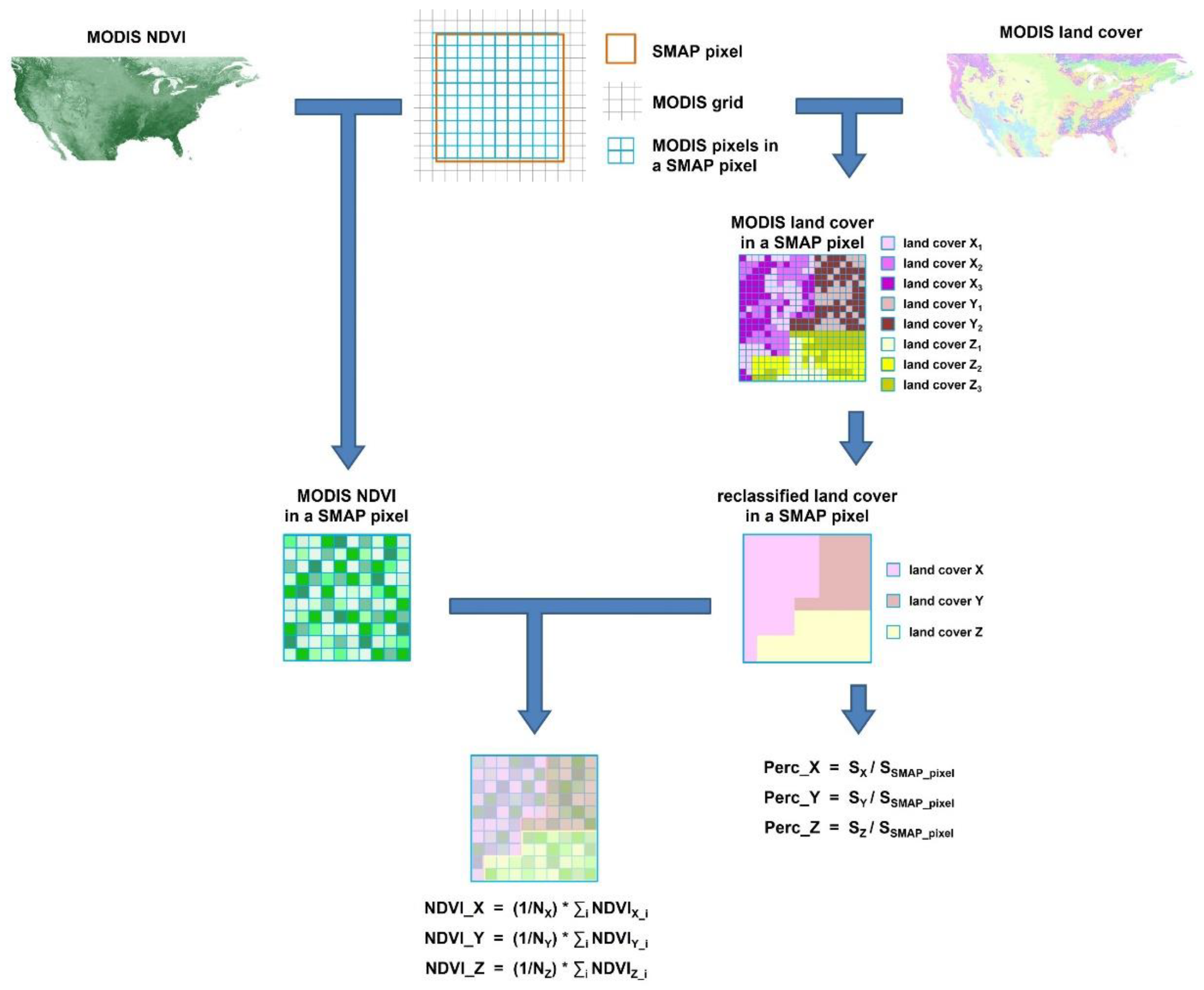
2.3.2. Multi-Source Data Preprocessing

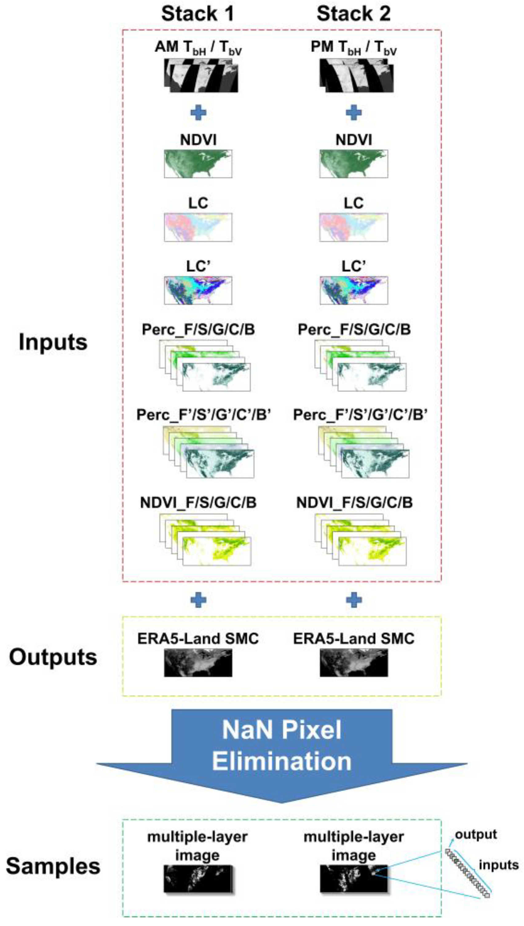
Moreover, for SMAP data on each date, the brightness temperatures of both AM and PM overpasses were examined according to the quality assessment layers. The pixels with values beyond the physical range and suffering from radio frequency interference (RFI) were removed. As is laid out in some works, on a scale of passive microwave pixels, the average SMC in a pixel is relatively stable daily [42,43]. Hence, we applied the instantaneous SMAP brightness temperature to retrieve the daily mean SMC in this study. Then, a grid vector layer was established in line with the SMAP pixels of the study area (293 rows by 712 columns), which was further applied for data resampling in the following steps.

For MCD12Q1 data, pixels of water bodies, wetlands, urban areas, ice, and snow were masked because they were outside the range of the study. Then, two means of data preprocessing were conducted. One was that the masked MCD12Q1 classification data, 13 classes in total, were resampled into the SMAP grid by finding the class of the most pixels (MCD12Q1) in each SMAP pixel and assigning it to the corresponding SMAP pixel. The other was that the masked MCD12Q1 classification data were reclassified into five typical land cover classes, i.e., forests, shrublands, grasslands, croplands, and barren. For each SMAP pixel, the percentages of these five typical classes were calculated and designated as Perc_F, Perc_S, Perc_G, Perc_C, and Perc_B, respectively.

Table 1. Comparison between MCD12Q1 IGBP classes and reclassified typical classes.

MCD12Q1 IGBP Classes	Reclassified Typical Classes
Evergreen Needleleaf Forests	Forests
Evergreen Broadleaf Forests
Deciduous Needleleaf Forests
Deciduous Broadleaf Forests
Mixed Forests
Closed Shrublands	Shrublands
Open Shrublands
Woody Savannas	Grasslands
Savannas
Grasslands
Croplands	Croplands
Cropland/Natural Vegetation Mosaics
Barren	Barren
Permanent Wetlands (Eliminated) Urban and Built-up Lands (Eliminated)	Others (Eliminated)
Water Bodies (Eliminated)
Permanent Snow and Ice (Eliminated)

lists the land cover classes of MCD12Q1 and the corresponding reclassified typical classes.

For MOD/MYD13A2 data, after removing the invalid pixels on each date, the NDVI data were averaged as the daily mean NDVI. Like the MCD12Q1 data, two methods of NDVI data preprocessing were performed. One was that the daily mean NDVI was resampled into the SMAP grid by averaging the values within each pixel. The other was that the daily mean NDVI was matched spatially with the reclassified MCD12Q1 land cover data gained in the preceding step. The average NDVIs corresponding to the five typical land cover classes were calculated. The five average NDVIs were designated as NDVI_F, NDVI_S, NDVI_G, NDVI_C, and NDVI_B, corresponding to the five typical classes of “forests”, “shrublands”, “grasslands”, “croplands”, and “barren”, respectively.

Figure 2 illustrates the calculation of “percentages of typical land cover classes” and “average NDVIs corresponding to typical land cover classes” in a SMAP pixel. Here, the details in one SMAP pixel are displayed for better explanation. For example, X₁, X₂, and X₃ are land cover classes in MODIS land cover data (MCD12Q1). Supposedly, according to the reclassification scheme stated above, they belong to one of the typical classes, X. Then, the percentage of the typical class X in the SMAP pixel is calculated as the area of X (S_X, equal to the sum area of X₁, X₂, and X₃ in MODIS land cover data) divided by the area of the SMAP pixel (S_{SMAP_pixel}), while the average NDVI corresponding to the typical class X in the SMAP pixel is calculated as the sum of NDVI values corresponding to X land cover class (Σ_iNDVI_{X_i}, i = 1, 2, …, N_X) divided by the number of pixels corresponding to X land cover class (N_X). Relevant variables for land cover Y and Z can also be calculated.

For GLC_FCS30 data, the preprocessing method was similar to MCD12Q1 data. Firstly, the data covering the study area were selected, and pixels of water bodies, wetlands, urban areas, ice, and snow were masked. Then, the masked GLC_FCS30 data (25 classes in total) were resampled into the SMAP grid; also, the data were reclassified into the five typical land cover classes. For each SMAP pixel, the percentages of these five typical classes were also calculated and designated as Perc_F’, Perc_S’, Perc_G’, Perc_C’, and Perc_B’, respectively.

Table 2. Comparison between GLC_FCS30 classes and reclassified typical classes.

GLC_FCS30 Classes	Reclassified Typical Classes
Open evergreen broad-leaved forest	Forests
Closed evergreen broad-leaved forest
Open deciduous broad-leaved forest
Closed deciduous broad-leaved forest
Open evergreen needle-leaved forest
Closed evergreen needle-leaved forest
Open deciduous needle-leaved forest
Closed deciduous needle-leaved forest
Open mixed-leaf forest
Closed mixed-leaf forest
Shrubland	Shrublands
Evergreen shrubland
Deciduous shrubland
Grassland	Grasslands
Lichens and mosses
Rainfed cropland	Croplands
Herbaceous cover
Tree or shrub cover (orchard)
Irrigated cropland
Sparse vegetation	Barren
Sparse shrubland
Sparse herbaceous
Bare areas
Consolidated bare areas
Unconsolidated bare areas
Wetlands (eliminated)	Others (eliminated)
Impervious surfaces (eliminated)
Water body (eliminated)
Permanent ice and snow (eliminated)

lists the land cover classes of GLC_FCS30 and the corresponding reclassified typical classes. Note that although both MCD12Q1 and GLC_FCS30 data were resampled into the SMAP resolution, the latter has a higher original resolution than the former. The following sections provide and discuss the differences in retrieving outcomes between these two land cover data as input parameters.

For ERA5-Land models SMC, the data in the study area was extracted and resampled into the SMAP grid, and the SMC values of all 24 h in each date of interest were averaged as the output parameter of the samples for the random forest model.

2.3.3. Sample Pools

When multi-source data were prepared, they all took the form of raster layers of 293 rows by 712 columns with spatial resolution in line with SMAP data, including:

• SMAP brightness temperature of AM overpasses (AM T_bH/T_bV);
• SMAP brightness temperature of PM overpasses (PM T_bH/T_bV);
• Resampled NDVI (NDVI);
• Resampled land cover derived from MCD12Q1 (LC);
• Resampled land cover derived from GLC_FCS30 (LC’);
• “percentages of the typical land cover classes” in a SMAP pixel derived from MCD12Q1 (Perc_F/S/G/C/B);
• “percentages of the typical land cover classes” in a SMAP pixel derived from GLC_FCS30 (Perc_F’/S’/G’/C’/B’);
• “average NDVIs corresponding to the typical land cover classes” in a SMAP pixel (NDVI_F/S/G/C/B);
• Resampled ERA5-Land modeled SMC.

Then, these raster layers on each date of interest were stacked to construct the samples. The ERA5-Land modeled SMC was set as the output parameter and the others as input parameters. Furthermore, for SMAP brightness temperature data, there are two overpasses in a day at local time (6 a.m./6 p.m.), which also differ in footprints and distribution of available observations. Therefore, setting brightness temperatures of AM/PM overpasses as input parameters may bring about discrepancies in SMC retrieval. Two stacking methods were used to investigate this discrepancy (presented in Figure 3). In Stacks 1, the brightness temperatures of AM overpasses were used, whereas in Stacks 2, the brightness temperatures of PM overpasses were used. After layer stacking, the “NaN pixel elimination” procedure was conducted. As mentioned above, there were some invalid data for each raster layer, such as RFI pixels in AM/PM T_bH/T_bV layers and water body pixels in land cover layers. The pixels containing invalid data in one or more layers should be eliminated because they could not form integrated samples. Therefore, the remaining pixels with data from all valid layers were retained and ready for sample formation.

Next, three scenarios with respective sample pools were established by gathering samples of different dates of interest and stacking methods in a particular manner.

Table 3. Three scenarios with corresponding stacking methods, SMAP data, and numbers of samples.

Scenario	Method of Stacking	SMAP Tb Data	Number of Samples
1	Stack 1	AM overpasses	956,677
2	Stack 2	PM overpasses	972,188
3	Stack 1 and Stack 2	AM and PM overpasses	1,928,865

lists the details of three scenarios in this study. Scenarios 1 and 2 correspond to the samples formed by two stacking methods (Stack 1 and 2); Scenario 3 corresponds to the union of samples in Scenarios 1 and 2. The samples in each corresponding sample pool were randomly divided into training/testing samples at 90%/10% for each scenario. In fact, in relevant studies, the proportion of training samples to testing samples may vary [44,45,46]. In this study, as a large number of samples for training were expected, we deemed it reasonable to allocate 90% of the samples to train the random forest algorithm. The training/testing samples were used for random forest training and testing in the following steps, where the random forest training and SMC retrieval with different scenarios and input parameter combinations were implemented, and the estimated SMC values of testing samples acquired by the trained random forest algorithm were compared with their output parameters (ERA5-Land modeled SMC). The agreement was evaluated by the statistical metrics, which are specified in the following text.

2.3.4. Input Parameter Combinations

A couple of input parameter combinations were proposed to determine the influence of various input parameters on SMC retrieval, as shown in

Table 4. Input combinations for RF SMC retrieval.

Combination	1	2	3	4	5	6	7
Input Parameters	TbH TbV	TbH TbV	TbH TbV	TbH TbV	TbH TbV	TbH TbV	TbH TbV
	NDVI	NDVI	NDVI	NDVI	NDVI	NDVI_F NDVI_S NDVI_G NDVI_C NDVI_B	NDVI_F NDVI_S NDVI_G NDVI_C NDVI_B
		LC	LC’	Perc_F Perc_S Perc_G Perc_C Perc_B	Perc_F’ Perc_S’ Perc_G’ Perc_C’ Perc_B’		Perc_F’ Perc_S’ Perc_G’ Perc_C’ Perc_B’

. Since this study mainly focuses on the influence of vegetation condition and land use on SMC retrieval with passive microwave data, only relevant variables were considered to exclude interference from other factors. To be specific, for Combinations 1~5, we separately added NDVI, LC, LC’, Perc_F/S/G/C/B, and Perc_F’/S’/G’/C’/B’ to the brightness temperature; for Combination 6, the NDVI in Combination 1 was substituted with NDVI_F/S/G/C/B; for Combination 7, Perc_F’/S’/G’/C’/B’ and NDVI_F/S/G/C/B were utilized to represent NDVI and land cover characteristics. All seven combinations were applied to random forest models to finish SMC retrieval processes for each of the three scenarios mentioned in the previous section. The influence of proposed input parameters was analyzed by comparing the statistical metrics. Moreover, the analyses of the AM/PM brightness temperature selection and training/testing sample-allocating methods were achieved by comparing SMC retrieving outcomes between the scenarios.

2.3.5. Statistical Metrics

The SMC retrieving accuracy was evaluated using two statistical metrics: the unbiased root mean square error (ubRMSE) and the correlation coefficient (r), which can be expressed as follows:

$$\mathrm{u}\mathrm{b}\mathrm{R}\mathrm{M}\mathrm{S}\mathrm{E}=\sqrt{{\displaystyle \frac{1}{n}}\sum _{i=1}^n{\left({SMC}_i-{\widehat{SMC}}_i\right)}^2-{\left({\displaystyle \frac{1}{n}}\sum _{i=1}^n\left({SMC}_i-{\widehat{SMC}}_i\right)\right)}^2},$$

(1)

$$r={\displaystyle \frac{{\sum }_{i=1}^n\left({SMC}_i-\overline{SMC}\right)\left({\widehat{SMC}}_i-\overline{\widehat{SMC}}\right)}{\sqrt{{\sum }_{i=1}^n{\left({SMC}_i-\overline{SMC}\right)}^2}\sqrt{{\sum }_{i=1}^n{\left({\widehat{SMC}}_i-\overline{\widehat{SMC}}\right)}^2}}}.$$

(2)

where n is the number of samples, ${SMC}_i$ represents the ith sample’s in situ SMC, $\overline{SMC}$ Represents mean in situ SMC values of the relevant samples, ${\widehat{SMC}}_i$ represents the ith sample’s estimated SMC value, and $\overline{\widehat{SMC}}$ represents the mean estimated SMC values of all the relevant samples.

3. Results

At first, it should be clarified that random allocations of training/testing samples may lead to variant SMC retrieval outcomes [47,48], so for each round of random forest training/testing, we repeated the training/testing process ten times, and the average SMC retrieval performance was assessed.

Table 5. The SMC retrieval’s correlation coefficients (r) with Combination 1~7 input parameters in each scenario. The values in bold suggest the combinations with the best statistical metrics for each scenario. In contrast, the underlined values suggest the scenarios with the highest statistical metric improvement for each combination in Combinations 2~7 compared with Combination 1.

r	Combination 1	Combination 2	Combination 3	Combination 4	Combination 5	Combination 6	Combination 7
Scenario 1	0.797	0.813	0.817	0.826	0.897	0.816	0.909
Scenario 2	0.805	0.823	0.825	0.837	0.903	0.828	0.914
Scenario 3	0.796	0.813	0.816	0.834	0.910	0.819	0.923

and

Table 6. SMC retrieval’s unbiased root mean square error (ubRMSE) with a combination of 1~7 input parameters in each scenario. The values in bold suggest the combinations with the best statistical metrics for each scenario. In contrast, the underlined values suggest the scenarios with the highest statistical metric improvement for each combination in Combination 2~7 compared with Combination 1.

ubRMSE (cm3cm−3)	Combination 1	Combination 2	Combination 3	Combination 4	Combination 5	Combination 6	Combination 7
Scenario 1	0.0761	0.0733	0.0726	0.0709	0.0557	0.0726	0.0526
Scenario 2	0.0757	0.0726	0.0722	0.0696	0.0551	0.0715	0.0522
Scenario 3	0.0767	0.0738	0.0733	0.0700	0.0528	0.0726	0.0490

list the statistical metrics, i.e., r and ubRMSE of SMC retrieval with Combination 1~7 input parameters in each scenario.

3.1. Results of Combinations 1, 2, and 3

Concerning Combinations 1, 2, and 3, the latter two combinations can be regarded as adding a land cover variable based on Combination 1. Using Combinations 2 and 3 as input parameters for all scenarios generally yielded more accurate SMC estimations than using Combination 1. Explicitly speaking, compared with Combination 1, Combination 2 improved the retrieving accuracy most in Scenario 2, with r rising by 0.018 (from 0.805 to 0.823) and ubRMSE declining by 0.0031 cm³cm⁻³ (from 0.0757 cm³cm⁻³ to 0.0726 cm³cm⁻³); similarly, Combination 3 improved the retrieving accuracy most in Scenarios 1 and 2, with r rising by 0.020 and ubRMSE declining by 0.0035 cm³cm⁻³. Nevertheless, in most scenarios, the improvements of Combination 3 in r were more favorable than those of Combination 2. This indicated that although the GLC_FCS30 and the MCD12Q1 were upscaled to SMAP-pixel resolution, the GLC_FCS30, with initially higher resolution, performed better than the MCD12Q1 in SMC retrieval.

3.2. Results of Combinations 4 and 5

As for Combinations 4 and 5, a series of variables rather than a sole land cover variable were added based on Combination 1. Comparing the outcomes of Combination 4 and Combination 1, the r rose at most by 0.038 (from 0.796 to 0.834) in Scenario 3, and ubRMSE declined at most by 0.0067 cm³cm⁻³ (from 0.0767 cm³cm⁻³ to 0.0700 cm³cm⁻³) in Scenario 3 as well; for Combination 5, the maximum rise of r was 0.114, and the ultimate decline of ubRMSE was 0.0239 cm³cm⁻³ (both in Scenario 3) compared with Combination 1. The SMC retrieving accuracy improvements of Combinations 4 and 5 over Combination 1 were more pronounced than those of Combinations 2 and 3.

3.3. Results of Combinations 6 and 7

As for Combination 6, substituting NDVI with average NDVIs corresponding to the five typical classes improved SMC retrieval accuracy. The best improvement occurred again in Scenario 2, with the r rising by 0.023 and the ubRMSE declining by 0.0042 cm³cm⁻³.

Combination 7 synthesized “the percentages of typical land cover classes” derived from GLC_FCS30 (which had performed best in improving SMC retrieval among these land cover-related variables) and “average NDVIs corresponding to the typical land cover classes” with the brightness temperature parameters. The results showed that Combination 7 achieved the highest SMC retrieval accuracy among all input combinations. Hence, in this study, the optimized input combination is Combination 7. The highest rise of r is 0.127, and the maximum decline of ubRMSE is 0.0277 cm³cm⁻³ (both in Scenario 3).

3.4. Comparison of Scenarios 1, 2, and 3

To investigate the performances of AM and PM brightness temperatures as the input parameters, we compared Scenarios 1/2/3 jointly in each combination. The results showed variant performances of those three scenarios. Concerning the absolute values of statistical metrics in each combination or the relative improvement for Combinations 2~7 compared with Combination 1, there is no sign that one particular scenario outperformed the others.

4. Discussion

4.1. The Influence of Land Cover Variables as Input Parameters

Previous studies have claimed that land cover influences soil hydraulic attributes and SMC distribution [49,50,51]. The interaction between land cover and microwave signals is particularly significant, as it directly impacts the dynamic range of microwave measurements [52,53,54]. This interaction can introduce variability and bias into SMC estimates if not adequately accounted for. In this study, in terms of the result comparison between Combination 1 and Combinations 2/3, it was shown that adding the land cover variable as an input parameter was beneficial to SMC retrieval. Moreover, the SMC retrieving results of Combinations 4 and 5 implies that the degree of accuracy improvement correlated with the elaborateness of description of the details of spatial characteristics in a pixel.

It was proven in some studies that at the small catchment scale (about 3~6 km²), land cover played a significant role in the spatial distribution and temporal dynamics of SMC. Zucco et al. [55] pointed out that in the study area in central Italy with the main land cover types of croplands and woodlands, higher soil moisture variability was observed at the catchment scale, which could be attributed to the difference in land covers. Fu et al. [56] focused on the effects of land use on soil moisture variation in a small catchment on the Loess Plateau in China. It was found that different land uses responded to the precipitation differently, with woodland and intercropping land showing a lag effect following a rain event and shrubland registering lower mean soil moisture owing to local shrubs’ deep and enormous roots. In this study, the scale of SMAP pixels is larger than the scale of these small catchments in previous studies, and various land cover types may be contained in one SMAP pixel. We calculated the percentage composition of five typical land cover classes within each SMAP pixel to address this. Incorporating these detailed land cover proportions as input parameters provided a more nuanced representation of the land surface’s hydrological characteristics. This enhanced input parameter facilitated a more precise depiction of the relationships between inputs and outputs during the random forest training process, and improved SMC retrieving accuracy could be expected.

Additionally, the percentages of the typical classes proposed in this study were calculated based on the reclassified results of MCD12Q1 and GLC_FCS30. Concerning the number of land cover classes, the newly proposed variables (five classes) seem to be a generalization of land cover information derived from MCD12Q1 (13 classes) and GLC_FCS30 (25 classes). Still, conversely, the performances on SMC retrieval verify the effect of variable spatial optimization.

4.2. The Influence of NDVI Variables as Input Parameter

NDVI is a frequently used variable denoting the growth condition of land surface vegetation, which is often assigned as the contribution of vegetation to microwave signals and plays a vital role in the models for SMC retrieval [57,58]. The relationship between NDVI and land cover types is also an indispensable factor affecting SMC retrieval. In the study of Han et al. [59], the researchers utilized MODIS data products of land surface temperature (LST), NDVI, and land cover to estimate the spatial and temporal changes in soil moisture status. By comparing the temperature–vegetation dryness index (TVDI, an index calculated with NDVI and LST) with the land cover types in the great Changbai Mountains study area, the considerable relationship among soil moisture condition, NDVI, and land cover types was demonstrated.

Moreover, in most SMAP pixels, multiple land covers may commonly exist, and each land cover type is characterized by its unique NDVI temporal profile and corresponding SMC patterns. Accurately representing the NDVI dynamics associated with each land cover class within an SMAP pixel is crucial for practical model training and accurate SMC retrieval. Consequently, for the study area where mixed SMAP pixels are dominant, incorporating multiple NDVI values, each representing one of the five typical land cover classes within the pixel, provided a more comprehensive characterization of the NDVI features associated with different land cover types. This approach enhanced the model’s ability to capture the complex relationships between land cover, NDVI, and SMC, ultimately improving SMC retrieval accuracy.

4.3. The Performances of AM and PM Brightness Temperatures as the Input Parameter

Some earlier studies argued that AM overpasses were proper for SMC retrieval since the assumptions of thermal equilibrium and near uniformity of conditions in the land surface were more likely to be true at 6 a.m. than at 6 p.m. [60,61,62]. In this study, however, we did not obtain consistent results, and the data of AM overpasses did not necessarily bring about higher SMC retrieving accuracy. This discrepancy may be attributed to two primary factors: (1) real-world conditions are more complex than theoretical assumptions than assumptions of physics; second, only the region of North America was paid attention to instead of the global land surface, possibly leading to the inconsistency in data preference with the existing research.

4.4. Limitations and Future Directions

Although the results indicated the effectiveness of introducing the spatially optimized variables and the mechanism analyzed and discussed above, several problems remain to be resolved. For example, we verified the method only in a study area in North America with various topographical and climatic features. Further experiments are required to investigate the feasibility of this method in other places, and passive microwave RS data of multi-frequency and multiple incidence angles (such as AMSR-2 and SMOS) can also be utilized to explore the proposed method’s applicability. Moreover, it is suggested in Zhang’s work [63] that machine/deep-learning-based models with physical interpretation should be developed. For example, Singh and Gaurav [64] introduced a learning bias physics-informed machine learning (PIML) model for estimating surface SMC, integrating physics into the loss function of a fully connected feed-forward neural network (FFNN). Chavoshi et al. [65] proposed a physics-informed neural network (PINN) model that estimates the vadose zone SWC profile by incorporating Richardson’s equation. These works provide a fresh perspective on incorporating physical knowledge into empirical models, which is worth our reference in future research.

5. Conclusions

The method of variable spatial optimization in SMC retrieval using an RF model was discussed in this study. New variables characterizing detailed information of coarse passive microwave pixels, i.e., “percentages of typical land cover classes” and “average NDVIs corresponding to typical land cover classes”, were proposed as the input parameters. Variables such as SMAP brightness temperature, NDVI, land cover, and ERA5-Land SMC were combined to construct samples, and the random forest was chosen as the retrieving algorithm.

The results proved that adding land cover variables as input parameters was conducive to improving SMC retrieving accuracy. Adding the percentages of typical land cover classes in SMAP pixels as input parameters could gain more favorable outcomes. The maximum rise of r was 0.114, and the maximum decline of ubRMSE was 0.0239 cm³cm⁻³ (after adding Perc_F’/S’/G’/C’/B’). Meanwhile, replacing NDVI with average NDVIs corresponding to the typical land cover classes in SMAP pixels also enhanced the SMC retrieving performances in all scenarios, with the maximum rise of r by 0.023 and the decline of ubRMSE by 0.0042 cm³cm⁻³. The effectiveness of variable spatial optimization was testified to. In addition, the performance of AM and PM brightness temperatures as input parameters was also analyzed.

This study has revealed the feasibility of parameter optimization in coarse pixels for SMC retrieval with passive microwave data and RF algorithms. By involving detailed information in these coarse pixels, the characteristics of land cover and NDVI are better presented, the quality of model training is enhanced, and SMC retrieving accuracy can be improved.

References

1. Chen, W.; Li, Z.; Jiao, L.; Wang, C.; Gao, G.; Fu, B. Response of soil moisture to rainfall event in black locust plantations at different stages of restoration in hilly-gully area of the Loess Plateau, China. Chin. Geogr. Sci. 2020, 30, 427–445. [Google Scholar] [CrossRef]
2. Robinson, D.A.; Campbell, C.S.; Hopmans, J.W.; Hornbuckle, B.K.; Jones, S.B.; Knight, R.; Ogden, F.; Selker, J.; Wendroth, O. Soil moisture measurement for ecological and hydrological watershed-scale observatories: A review. Vadose Zone J. 2008, 7, 358–389. [Google Scholar] [CrossRef]
3. Edokossi, K.; Jin, S.; Mazhar, U.; Molina, I.; Calabia, A.; Ullah, I. Monitoring the drought in Southern Africa from space-borne GNSS-R and SMAP data. Nat. Hazards. 2024, 120, 7947–7967. [Google Scholar] [CrossRef]
4. Topp, G.C. The application of time-domain reflectometry (TDR) to soil water content measurement. In Proceedings of the International Conference on Measurement of Soil and Plant Water Status, Utah State University, Logan, UT, USA, 6–10 July 1987. [Google Scholar]
5. Reynolds, S.G. The gravimetric method of soil moisture determination Part I A study of equipment, and methodological problems. J. Hydrol. 1970, 11, 258–273. [Google Scholar] [CrossRef]
6. Jackson, T.J.; Bindlish, R.; Cosh, M.H.; Zhao, T.; Starks, P.J.; Bosch, D.D.; Seyfried, M.; Moran, M.S.; Goodrich, D.C.; Kerr, Y.H.; et al. Validation of Soil Moisture and Ocean Salinity (SMOS) soil moisture over watershed networks in the US. IEEE Trans. Geosci. Remote Sens. 2011, 50, 1530–1543. [Google Scholar] [CrossRef]
7. Han, L.; Wang, C.; Yu, T.; Gu, X.; Liu, Q. High-precision soil moisture mapping based on multi-model coupling and background knowledge, over vegetated areas using Chinese Gf-3 and GF-1 satellite data. Remote Sens. 2020, 12, 2123. [Google Scholar] [CrossRef]
8. Chen, S.; Zhao, K.; Jiang, T.; Li, X.; Zheng, X.; Wan, X.; Zhao, X. Predicting surface roughness and moisture of bare soils using multi-band spectral reflectance under field conditions. Chin. Geogr. Sci. 2018, 28, 986–997. [Google Scholar] [CrossRef]
9. Li, Z.L.; Leng, P.; Zhou, C.; Chen, K.S.; Zhou, F.C.; Shang, G.F. Soil moisture retrieval from remote sensing measurements: Current knowledge and directions for the future. Earth Sci. Rev. 2021, 218, 103673. [Google Scholar] [CrossRef]
10. Zeng, J. Soil Moisture Retrieval in the Tibetan Plateau Using Passive Microwave Remote Sensing Observations. Ph.D. Dissertation, Chinese Academy of Sciences, Beijing, China, 2015. [Google Scholar]
11. Ma, H.; Zeng, J.; Chen, N.; Zhang, X.; Cosh, M.H.; Wang, W. Satellite surface soil moisture from SMAP, SMOS, AMSR2 and ESA CCI: A comprehensive assessment using global ground-based observations. Remote Sens. Environ. 2019, 231, 111215. [Google Scholar] [CrossRef]
12. Kim, H.; Wigneron, J.P.; Kumar, S.; Dong, J.; Wagner, W.; Cosh, M.H.; Bosch, D.D.; Collins, C.H.; Starks, P.J.; Seyfried, M.; et al. Global scale error assessments of soil moisture estimates from microwave-based active and passive satellites and land surface models over forest and mixed irrigated/dryland agriculture regions. Remote Sens. Environ. 2020, 251, 112052. [Google Scholar] [CrossRef]
13. Fung, A.K.; Li, Z.; Chen, K.S. Backscattering from a randomly rough dielectric surface. IEEE Trans. Geosci. Remote Sens. 1992, 30, 356–369. [Google Scholar] [CrossRef]
14. Chen, K.S.; Wu, T.D.; Tsang, L.; Li, Q.; Shi, J.; Fung, A.K. Emission of rough surfaces calculated by the integral equation method with comparison to three-dimensional moment method simulations. IEEE Trans. Geosci. Remote Sens. 2003, 41, 90–101. [Google Scholar] [CrossRef]
15. Choudhury, B.J.; Schmugge, T.J.; Chang, A.; Newton, R.W. Effect of surface roughness on the microwave. J. Geophys. Res. 1979, 84, 5699–5706. [Google Scholar] [CrossRef]
16. Mo, T.; Choudhury, B.J.; Schmugge, T.J.; Wang, J.R.; Jackson, T.J. A model for microwave emission from vegetation-covered fields. J. Geophys. Res. Oceans 1982, 87, 11229–11237. [Google Scholar] [CrossRef]
17. Song, P. Improved Surface Soil Moisture Estimation Methods and Their Applications Based on AMSR Radiometers. Ph.D. Dissertation, Zhejiang University, Hangzhou, China, 2019. [Google Scholar]
18. Karthikeyan, L.; Pan, M.; Wanders, N.; Kumar, D.N.; Wood, E.F. Four decades of microwave satellite soil moisture observations: Part 1. A review of retrieval algorithms. Adv. Water Resour. 2017, 109, 106–120. [Google Scholar] [CrossRef]
19. Zheng, L.; Wu, M.; Xue, M.; Wu, H.; Liang, F.; Li, X.; Hou, S.; Liu, J. Power of SAR imagery and machine learning in monitoring Ulva Prolifera: A case study of Sentinel-1 and random forest. Chin. Geogr. Sci. 2024, 34, 1134–1143. [Google Scholar] [CrossRef]
20. Zhang, S.; Weng, F.; Yao, W. A multivariable approach for estimating soil moisture from Microwave Radiation Imager (MWRI). J. Meteorol. Res. 2020, 34, 732–747. [Google Scholar] [CrossRef]
21. Tong, C.; Wang, H.; Magagi, R.; Goïta, K.; Zhu, L.; Yang, M.; Deng, J. Soil moisture retrievals by combining passive microwave and optical data. Remote Sens. 2020, 12, 3173. [Google Scholar] [CrossRef]
22. Ma, H.; Zeng, J.; Zhang, X.; Peng, J.; Li, X.; Fu, P.; Cosh, M.H.; Letu, H.; Wang, S.; Chen, N.; et al. Surface soil moisture from combined active and passive microwave observations: Integrating ASCAT and SMAP observations based on machine learning approaches. Remote Sens. Environ. 2024, 308, 114197. [Google Scholar] [CrossRef]
23. Meng, Q.; Zhang, L.; Xie, Q.; Yao, S.; Chen, X.; Zhang, Y. Combined use of GF-3 and Landsat-8 satellite data for soil moisture retrieval over agricultural areas using artificial neural network. Adv. Meteorol. 2018, 2018, 9315132. [Google Scholar] [CrossRef]
24. Ma, C.; Li, X.; Wei, L.; Wang, W. Multi-scale validation of SMAP soil moisture products over cold and arid regions in northwestern China using distributed ground observation data. Remote Sens. 2017, 9, 327. [Google Scholar] [CrossRef]
25. Zhang, L.; Zhang, Z.; Xue, Z.; Li, H. Sensitive feature evaluation for soil moisture retrieval based on multi-source remote sensing data with few in-situ measurements: A case study of the Continental U.S. Water 2021, 13, 2003. [Google Scholar] [CrossRef]
26. Qu, Y.; Zhu, Z.; Chai, L.; Liu, S.; Montzka, C.; Liu, J.; Yang, X.; Lu, Z.; Jin, R.; Li, X.; et al. Rebuilding a microwave soil moisture product using random forest adopting AMSR-E/AMSR2 brightness temperature and SMAP over the Qinghai–Tibet Plateau, China. Remote Sens. 2019, 11, 683. [Google Scholar] [CrossRef]
27. Bai, X.; Zeng, J.; Chen, K.S.; Li, Z.; Zeng, Y.; Wen, J.; Wang, X.; Dong, X.; Su, Z. Model by integration of global sensitivity analysis using SMAP active and passive observations. IEEE Trans. Geosci. Remote Sens. 2018, 57, 1084–1099. [Google Scholar] [CrossRef]
28. Zeng, J.; Shi, P.; Chen, K.S.; Ma, H.; Bi, H.; Cui, C. On the relationship between radar backscatter and radiometer brightness temperature from SMAP. IEEE Trans. Geosci. Remote Sens. 2021, 60, 1–16. [Google Scholar] [CrossRef]
29. Ge, L.; Hang, R.; Liu, Y.; Liu, Q. Comparing the performance of neural network and deep convolutional neural network in estimating soil moisture from satellite observations. Remote Sens. 2018, 10, 1327. [Google Scholar] [CrossRef]
30. Kolassa, J.; Gentine, P.; Prigent, C.; Aires, F. Soil moisture retrieval from AMSR-E and ASCAT microwave observation synergy. Part 1: Satellite data analysis. Remote Sens. Environ. 2016, 173, 1–14. [Google Scholar] [CrossRef]
31. Kolassa, J.; Gentine, P.; Prigent, C.; Aires, F.; Alemohammad, S.H. Soil moisture retrieval from AMSR-E and ASCAT microwave observation synergy. Part 2: Product evaluation. Remote Sens. Environ. 2017, 195, 202–217. [Google Scholar] [CrossRef]
32. Muñoz-Sabater, J.; Dutra, E.; Agustí-Panareda, A.; Albergel, C.; Arduini, G.; Balsamo, G.; Boussetta, S.; Choulga, M.; Harrigan, S.; Hersbach, H.; et al. ERA5-Land: A state-of-the-art global reanalysis dataset for land applications. Earth Syst. Sci. Data 2021, 13, 4349–4383. [Google Scholar] [CrossRef]
33. Hu, F.; Wei, Z.; Yang, X.; Xie, W.; Li, Y.; Cui, C.; Yang, B.; Tao, C.; Zhang, W.; Meng, L. Assessment of SMAP and SMOS soil moisture products using triple collocation method over Inner Mongolia. J. Hydrol. Reg. Stud. 2022, 40, 101027. [Google Scholar] [CrossRef]
34. Colliander, A.; Jackson, T.J.; Bindlish, R.; Chan, S.; Das, N.; Kim, S.B.; Cosh, M.H.; Dunbar, R.S.; Dang, L.; Pashaian, L.; et al. Validation of SMAP surface soil moisture products with core validation sites. Remote Sens. Environ. 2017, 191, 215–231. [Google Scholar] [CrossRef]
35. Chan, S.K.; Bindlish, R.; O’Neill, P.; Jackson, T.; Njoku, E.; Dunbar, S.; Chaubell, J.; Piepmeier, J.; Yueh, S.; Entekhabi, D.; et al. Development and assessment of the SMAP enhanced passive soil moisture product. Remote Sens. Environ. 2018, 204, 931–941. [Google Scholar] [CrossRef] [PubMed]
36. Colliander, A.; Reichle, R.H.; Crow, W.T.; Cosh, M.H.; Chan, S.; Das, N.N.; Bindlish, R.; Chaubell, J.; Kim, S.; Liu, Q.; et al. Validation of soil moisture data products from the NASA SMAP mission. IEEE J. Sel. Top. Appl. Earth Obs. Remote Sens. 2021, 15, 364–392. [Google Scholar] [CrossRef]
37. Wen, F.; Zhao, W.; Wang, Q.; Sánchez, N. A value-consistent method for downscaling SMAP passive soil moisture with MODIS products using self-adaptive window. IEEE Trans. Geosci. Remote Sens. 2019, 58, 913–924. [Google Scholar] [CrossRef]
38. Park, J.Y.; Ahn, S.R.; Hwang, S.J.; Jang, C.H.; Park, G.A.; Kim, S.J. Evaluation of MODIS NDVI and LST for indicating soil moisture of forest areas based on SWAT modeling. Paddy Water Environ. 2014, 12, 77–88. [Google Scholar] [CrossRef]
39. Zhang, X.; Liu, L.; Chen, X.; Gao, Y.; Xie, S.; Mi, J. GLC_FCS30: Global land-cover product with fine classification system at 30m using time-series Landsat imagery. Earth Syst. Sci. Data 2021, 13, 2753–2776. [Google Scholar] [CrossRef]
40. Breiman, L. Random forests. Mach. Learn. 2001, 45, 5–32. [Google Scholar] [CrossRef]
41. Zappa, L.; Forkel, M.; Xaver, A.; Dorigo, W. Deriving field scale soil moisture from satellite observations and ground measurements in a hilly agricultural region. Remote Sens. 2019, 11, 2596. [Google Scholar] [CrossRef]
42. Cui, C.; Xu, J.; Zeng, J.; Chen, K.S.; Bai, X.; Lu, H.; Chen, Q.; Zhao, T. Soil moisture mapping from satellites: An intercomparison of SMAP, SMOS, FY3B, AMSR2, and ESA CCI over two dense network regions at different spatial scales. Remote Sens. 2018, 10, 33. [Google Scholar] [CrossRef]
43. Zeng, J.; Shi, P.; Chen, K.S.; Ma, H.; Bi, H.; Cui, C. Assessment and error analysis of satellite soil moisture products over the third pole. IEEE Trans. Geosci. Remote Sens. 2022, 60, 1–18. [Google Scholar] [CrossRef]
44. Senyurek, V.; Lei, F.; Boyd, D.; Kurum, M.; Gurbuz, A.C.; Moorhead, R. Machine Learning-Based CYGNSS Soil Moisture Estimates over ISMN sites in CONUS. Remote Sens. 2020, 12, 1168. [Google Scholar] [CrossRef]
45. Rodríguez-Fernández, N.; de Rosnay, P.; Albergel, C.; Richaume, P.; Aires, F.; Prigent, C.; Kerr, Y. SMOS Neural Network Soil Moisture Data Assimilation in a Land Surface Model and Atmospheric Impact. Remote Sens. 2019, 11, 1334. [Google Scholar] [CrossRef]
46. Yang, Z.; Zhao, J.; Liu, J.; Wen, Y.; Wang, Y. Soil Moisture Retrieval Using Microwave Remote Sensing Data and a Deep Belief Network in the Naqu Region of the Tibetan Plateau. Sustainability 2021, 13, 12635. [Google Scholar] [CrossRef]
47. Holtgrave, A.K.; Förster, M.; Greifeneder, F.; Notarnicola, C.; Kleinschmit, B. Estimation of soil moisture in vegetation-covered floodplains with sentinel-1 SAR data using support vector regression. PFG–J. Photogram. Remote Sens. Geoinf. Sci. 2018, 86, 85–101. [Google Scholar]
48. Liu, Q.; Gu, X.; Chen, X.; Mumtaz, F.; Liu, Y.; Wang, C.; Yu, T.; Zhang, Y.; Wang, D.; Zhan, Y. Soil moisture content retrieval from remote sensing data by artificial neural network based on sample optimization. Sensors 2022, 22, 1611. [Google Scholar] [CrossRef]
49. Buczko, U.; Bens, O.; Huttl, R. Tillage effects on hydraulic properties and microporosity in silty and sandy soils. Soil Sci. Soc. Am. J. 2006, 70, 1998–2007. [Google Scholar] [CrossRef]
50. Vilasan, R.; Kapse, V. Evaluation of the prediction capability of AHP and F-AHP methods in flood susceptibility mapping of Ernakulam district (India). Nat. Hazards 2022, 112, 1767–1793. [Google Scholar] [CrossRef]
51. Zha, X.; Xiong, L.; Liu, C.; Shu, P.; Xiong, B. Identification and evaluation of soil moisture flash drought by a nonstationary framework considering climate and land cover changes. Sci. Total Environ. 2023, 856, 158953. [Google Scholar] [CrossRef]
52. Guerriero, L.; Ferrazzoli, P.; Vittucci, C.; Rahmoune, R.; Aurizzi, M.; Mattioni, A. L-band passive and active signatures of vegetated soil: Simulations with a unified model. IEEE J. Sel. Top. Appl. Earth Obs. Remote Sens. 2016, 9, 2520–2531. [Google Scholar] [CrossRef]
53. Liu, P.W.; Judge, J.; de Roo, R.D.; England, A.W.; Bongiovanni, T. Uncertainty in soil moisture retrievals using the SMAP combined active–passive algorithm for growing sweet corn. IEEE J. Sel. Top. Appl. Earth Obs. Remote Sens. 2016, 9, 3326–3339. [Google Scholar] [CrossRef]
54. Piles, M.; McColl, K.A.; Entekhabi, D.; Das, N.N.; Pablos, M. Sensitivity of Aquarius active and passive measurements temporal covariability to land surface characteristics. IEEE Trans. Geosci. Remote Sens. 2015, 53, 4700–4711. [Google Scholar] [CrossRef]
55. Zucco, G.; Brocca, L.; Moramarco, T.; Morbidelli, R. Influence of land use on soil moisture spatial–temporal variability and monitoring. J. Hydrol. 2014, 516, 193–199. [Google Scholar] [CrossRef]
56. Fu, B.; Wang, J.; Chen, L.; Qiu, Y. The effects of land use on soil moisture variation in the Danangou catchment of the Loess Plateau, China. Catena 2003, 54, 197–213. [Google Scholar] [CrossRef]
57. Das, N.N.; Entekhabi, D.; Dunbar, R.S.; Chaubell, M.J.; Yueh, S.; Jagdhuber, T.; Crow, W.; O’Neill, P.E.; Walker, J.P. The SMAP and Copernicus Sentinel 1A/B microwave active-passive high resolution surface soil moisture product. Remote Sens. Environ. 2019, 233, 111380. [Google Scholar] [CrossRef]
58. Ye, N.; Walker, J.P.; Gao, Y.; PopStefanija, I.; Hills, J. Comparison between thermal-optical and L-band passive microwave soil moisture remote sensing at farm scales: Towards UAV-based near-surface soil moisture mapping. IEEE J. Sel. Top. Appl. Earth Obs. Remote Sens. 2023, 17, 633–642. [Google Scholar] [CrossRef]
59. Han, Y.; Wang, Y.; Zhao, Y. Estimating Soil Moisture Conditions of the Greater Changbai Mountains by Land Surface Temperature and NDVI. IEEE Trans. Geosci. Remote Sens. 2010, 48, 2509–2515. [Google Scholar]
60. Chan, S.K.; Bindlish, R.; O’Neill, P.E.; Njoku, E.; Jackson, T.; Colliander, A.; Chen, F.; Burgin, M.; Dunbar, S.; Piepmeier, J.; et al. Assessment of the SMAP passive soil moisture product. IEEE Trans. Geosci. Remote Sens. 2016, 54, 4994–5007. [Google Scholar] [CrossRef]
61. Kolassa, J.; Reichle, R.H.; Liu, Q.; Alemohammad, S.H.; Gentine, P.; Aida, K.; Asanuma, J.; Bircher, S.; Caldwell, T.; Colliander, A.; et al. Estimating surface soil moisture from SMAP observations using a Neural Network technique. Remote Sens. Environ. 2018, 204, 43–59. [Google Scholar] [CrossRef]
62. Entekhabi, D.; Njoku, E.G.; O’Neill, P.E.; Kellogg, K.H.; Crow, W.T.; Edelstein, W.N.; Entin, J.K.; Goodman, S.D.; Jackson, T.J.; Johnson, J.; et al. The Soil Moisture Active Passive (SMAP) Mission. Proc. IEEE 2010, 98, 704–716. [Google Scholar] [CrossRef]
63. Zhang, Y.; Chen, Y.; Chen, L. A Two-Step Reconstruction Approach for High-Resolution Soil Moisture Estimates from Multi-Source Data. Water 2025, 17, 819. [Google Scholar] [CrossRef]
64. Singh, A.; Gaurav, K. PIML-SM: Physics-Informed Machine Learning to Estimate Surface Soil Moisture From Multisensor Satellite Images by Leveraging Swarm Intelligence. IEEE Trans. Geosci. Remote Sens. 2024, 62, 1–13. [Google Scholar] [CrossRef]
65. Chavoshi, A.; Dashtian, H.; Bakhshian, S.; Young, M.H.; Niyogi, D. PINN-SM: A Physics-Informed Neural Networks Model for Vadose Zone Soil Moisture Profile Prediction. arXiv 2024. [Google Scholar] [CrossRef]
Figure 1. Location of the study area.
Water 17 01604 g001
Figure 2. Illustration of calculating “percentages of typical land cover classes” and “average NDVIs corresponding to typical land cover classes”.
Water 17 01604 g002
Figure 3. Two methods of stacking raster layers for sample construction.
Water 17 01604 g003