Multi-Layer and Profile Soil Moisture Estimation and Uncertainty Evaluation Based on Multi-Frequency (Ka-, X-, C-, S-, and L-Band) and Quad-Polarization Airborne SAR Data from Synchronous Observation Experiment in Liao River Basin, China

Abstract

Validating the potential of multi-frequency synthetic aperture radar (SAR) data for multi-layer and profile soil moisture (SM) estimation modeling, we conducted an airborne multi-frequency SAR joint observation experiment (AMFSEX) over the Liao River Basin in China. The experiment simultaneously acquired airborne high spatial resolution quad-polarization (quad-pol) SAR data at five frequencies, including the Ka-, X-, C-, S-, and L-band. A preliminary “vegetation–soil” parameter estimation model based on the multi-frequency SAR data was established. Theoretical penetration depths of the multi-frequency SAR data were analyzed using the Dobson empirical model and the Hallikainen modified model. On this basis, a water cloud model (WCM) constrained by multi-polarization weighted and penetration depth weighted parameters was used to analyze the estimation accuracy of the multi-layer and profile SM (0–50 cm depth) under different vegetation types (grassland, farmland, and woodland). Overall, the estimation error (root mean square error, RMSE) of the surface SM (0–5 cm depth) ranged from 0.058 cm³/cm³ to 0.079 cm³/cm³, and increased with radar frequency. For multi-layer and profile SM (3 cm, 5 cm, 10 cm, 20 cm, 30 cm, 40 cm, 50 cm depth), the RMSE ranged from 0.040 cm³/cm³ to 0.069 cm³/cm³. Finally, a multi-input multi-output regression model (Gaussian process regression) was used to simultaneously estimate the multi-layer and profile SM. For surface SM, the overall RMSE was approximately 0.040 cm³/cm³. For multi-layer and profile SM, the overall RMSE ranged from 0.031 cm³/cm³ to 0.064 cm³/cm³. The estimation accuracy achieved by coupling the multi-source data (multi-frequency SAR data, multispectral data, and soil parameters) was superior to that obtained using the SAR data alone. The optimal SM penetration depth varied across different vegetation cover types, generally falling within the range of 10–30 cm, which holds true for both the scattering model and the regression model. This study provides methodological guidance for the development of multi-layer and profile SM estimation models based on the multi-frequency SAR data.

1. Introduction

Soil moisture (SM) refers to the water adsorbed onto soil particles and present in soil pores, primarily in liquid form, with a small portion existing as solid ice or gaseous water [1,2]. Although SM accounts for only 0.047% of the total available freshwater resources globally, it is one of the key variables in the global climate and weather systems [3,4]. SM plays a crucial role in the energy and water balance between the land surface and the atmosphere, participating in up to 20% of the entire water cycle [5]. SM directly determines the proportion of precipitation that is converted into evapotranspiration, infiltration, and runoff, making it a fundamental variable in the formation, transformation, and consumption of terrestrial water resources [6]. Additionally, SM is an essential condition for vegetation growth, influencing the rate of photosynthesis in plants and soil microbial respiration. An insufficient SM supply can hinder vegetation growth and development, indirectly affecting the sustainable development of regional ecosystems. Conversely, excessive SM can lead to soil hypoxia, further restricting root respiration and causing a decline in physiological functions or even plant death [7]. Therefore, real-time and accurate SM monitoring is of great significance for hydrological and ecological process attribution, agricultural water management, flood and drought emergency monitoring, timely and precise weather forecasting, and global climate change analysis [8,9].

Based on soil depth, SM can be broadly categorized into the following types: surface SM (SSM; 3 cm, 5 cm depth), near-surface SM (NSSM; 10 cm, 20 cm, 30 cm depth), and root-zone SM (RZSM; 40 cm, 50 cm depth). The profile SM represents the average water content within a specific vertical soil profile (e.g., 0–5 cm, 0–10 cm, 0–20 cm, 0–30 cm, 0–40 cm, and 0–50 cm) [10,11]. The temporal variations in SM at different depths play distinct roles in the “soil–vegetation–atmosphere” system, regulating various hydrometeorological, hydroclimatic, ecological, and biogeochemical processes across different spatial and temporal scales [8]. Generally, the SSM exhibits strong spatiotemporal variability due to direct atmospheric influences, such as precipitation and evaporation [12]. During precipitation events, the SSM gradually increases and eventually becomes saturated, with water infiltrating downward into the near-surface and root-zone soil layers. The distribution of root systems within the soil profile varies depending on land cover types (e.g., bare soil, farmland, grassland, shrubland, and woodland) [13,14,15]. Additionally, due to differences in growth stages, even the same vegetation type may exhibit varying root distribution patterns and water requirements across different phenological phases. Studies by Li et al. and Qian et al. have shown that vegetation productivity is particularly sensitive to deep SM [9,10]. In the early growth stage, when root systems are shallow, SSM plays a critical role in vegetation growth. In the later stages, as roots develop further, deep SM becomes increasingly important [7,16,17]. During this phase, even under meteorological drought conditions, the water retention capacity of the root-zone soil and the water absorption ability of plant roots can help vegetation survive short-term drought periods [13]. Therefore, multi-layer and profile SM monitoring over time is essential for understanding and predicting whether vegetation growth and development across different phenological stages are subjected to water stress.

Since the 1970s, spaceborne remote sensing technology has been increasingly used to obtain global-scale time-series SM data [12]. Active and passive microwave remote sensing are largely unaffected by cloud cover and precipitation, allowing for all-day, all-weather surface observations [4]. These methods primarily establish the relationship between soil dielectric properties, surface backscattering coefficients, brightness temperature characteristics, and SM content, making their physical basis relatively well-defined. However, the estimation models are complex and susceptible to interference from surface roughness and vegetation signals. The spatiotemporal accuracy of different SM estimation models is significantly influenced by regional factors, land cover types, and temporal selection, leading to inconsistencies in spatial and temporal precision [18,19,20,21]. Currently, the availability of extensive shared SM sensor networks, SM estimation algorithms, and time-series active and passive remote sensing satellite data presents unprecedented opportunities for large-scale multi-layer and profile SM mapping and applications [22,23,24]. Common satellite-based SM products include the Soil Moisture and Ocean Salinity (SMOS) mission, the Soil Moisture Active Passive (SMAP) mission, and the European Space Agency Climate Change Initiative SSM (ESA CCI SSM), which have become essential parameters in climate, meteorology, hydrology, ecology, and agriculture [25,26,27]. However, the existing SM products are primarily derived from passive microwave remote sensing data, which have relatively low spatial resolution, ranging from several kilometers to tens of kilometers, and are often limited to the SSM [28]. While some studies have improved the spatial and temporal resolution of these products through data fusion and downscaling techniques, their ability to support high-resolution SM monitoring remains insufficient [29]. The main sources of error in SM estimation using airborne or satellite-based remote sensing data include limitations of sensor parameters, signal interference from dense vegetation, soil surface roughness, surface heterogeneity, and climatic zone differences [10,17,30,31,32,33,34]. Therefore, it is necessary to incorporate prior surface knowledge to calibrate the SM estimation models, thereby improving both the accuracy and temporal robustness of the estimation results [35,36,37,38,39]. Another method for SM estimation and mapping is data assimilation [11,40]. This approach relies on Kalman filtering and a Bayesian framework to quantify retrieval errors and uncertainties. By integrating remote sensing estimates with hydrological models, and calibrating them using in situ measurements, it can achieve relatively high estimation accuracy. Commonly derived multi-layer and profile SM products include ERA5-Land (the fifth generation of ECMWF Atmospheric Reanalysis of the global climate—Land reanalysis), GLDAS (the Global Land Data Assimilation System), MERRA-2 (the Modern-Era Retrospective Analysis for Research and Applications, Version 2), CLDAS (China Land Data Assimilation System), and GLEAM (Global Land Evaporation Amsterdam Model) [41,42,43,44,45]. Although these data products offer high temporal resolution (ranging from several hours to a few days), their spatial resolution remains relatively low (0.1–0.5°) [46].

In recent years, the powerful nonlinear fitting capabilities of machine learning regression (MLR) algorithms have made them a promising tool for SM estimation modeling [11,31,47]. Compared to physically-based scattering models, data-driven regression models face considerable debate regarding their interpretability and transferability [31,38,48]. Most existing studies focus solely on the spatiotemporal interpolation accuracy of SM regression models, often overlooking their extrapolation capability across phase and space [10,11,17]. Given the substantial regional variability in the spatiotemporal distribution of SM, whether regression models trained on limited ground observation sites can accurately support SM mapping is critical for their deployment and practical application. As a result, an increasing number of researchers are exploring the spatiotemporal transferability of SM estimation models, aiming to enhance performance through multi-source data fusion, sensitivity-based feature augmentation, and coupling with physical scattering mechanisms [31,48,49].

Major research institutions worldwide have conducted large-scale SM “satellite–airborne–ground” synchronous observation experiments, primarily involving the United States, Canada, the European Union (EU), Australia, and China [33,46,50,51,52]. The United States and Canada have carried out calibration and validation experiments for satellite estimation and calibration models, including the Southern Great Plains Experiment 1999 (SGP99), the Soil Moisture Experiments in 2002 (SMEX02), the National Airborne Field Experiment (NAFE), the SMAP Validation Experiment in 2008/2012/2015 (SMAPVEX08/12/15), the SMAP Validation Experiment in 2016-Manitoba/Iowa (SMAPVEX16-MB/IA), the Canadian Experiment for Soil Moisture in 2010 (CanEx-SM10), and the Airborne Microwave Observatory of Subcanopy and Subsurface (AirMOSS) [50,53,54]. The EU has conducted calibration and validation experiments for the Sentinel and the Radar Observing System for Europe in L-band (ROSE-L) satellite series, including the Airborne SAR and Optics Campaigns for an Improved Monitoring of Agricultural Processes and Practices in 2006/2009 (AgriSAR2006/2009) and the Air- and Space-Borne C- and L-Band SAR for the Analysis of Soil and Plant Parameters in Agriculture in 2019 (SARSense2019) [51,55]. Australia has performed calibration and validation experiments for the SMOS and SMAP satellite missions, primarily including the Soil Moisture Active Passive Experiment-x (SMAPEx) and the Australian Airborne Cal/Val Experiment for SMOS-x (AACES) [56,57]. China has also conducted a series of comprehensive field measurement experiments, including the Heihe Watershed Allied Telemetry Experimental Research (HiWATER), the Luan River Basin Carbon/Water Cycle and Energy Balance Remote Sensing Experiment, and the Flash River Basin Water Cycle and Energy Balance Remote Sensing Experiment [46,58]. These large-scale field experiments have provided extensive and valuable ground-truth data, as well as synchronous satellite, airborne, and ground-based remote sensing observations. They serve as essential theoretical foundations and references for SM estimation modeling. Although some airborne experiments have acquired the multi-frequency SAR data, there is a lack of simultaneously measured multi-layer and profile SM data.

To validate the potential of the multi-frequency SAR data for multi-layer and profile SM estimation modeling, we conducted an airborne multi-frequency SAR joint observation experiment (AMFSEX) over the Liao River Basin in China. Based on this, this study primarily focuses on the following questions:

(1)

Compared with multi-spectral data, how do multi-frequency SAR data differ in characterizing vegetation biophysical parameters?

(2)

What are the differences in estimating SSM (0–5 cm) using multi-frequency SAR data?

(3)

How can multi-frequency SAR data be used to estimate the multi-layer and profile SM (0–50 cm)?

(4)

For different types of vegetation, what is the optimal penetration depth for SM estimation?

2. Study Area and Data

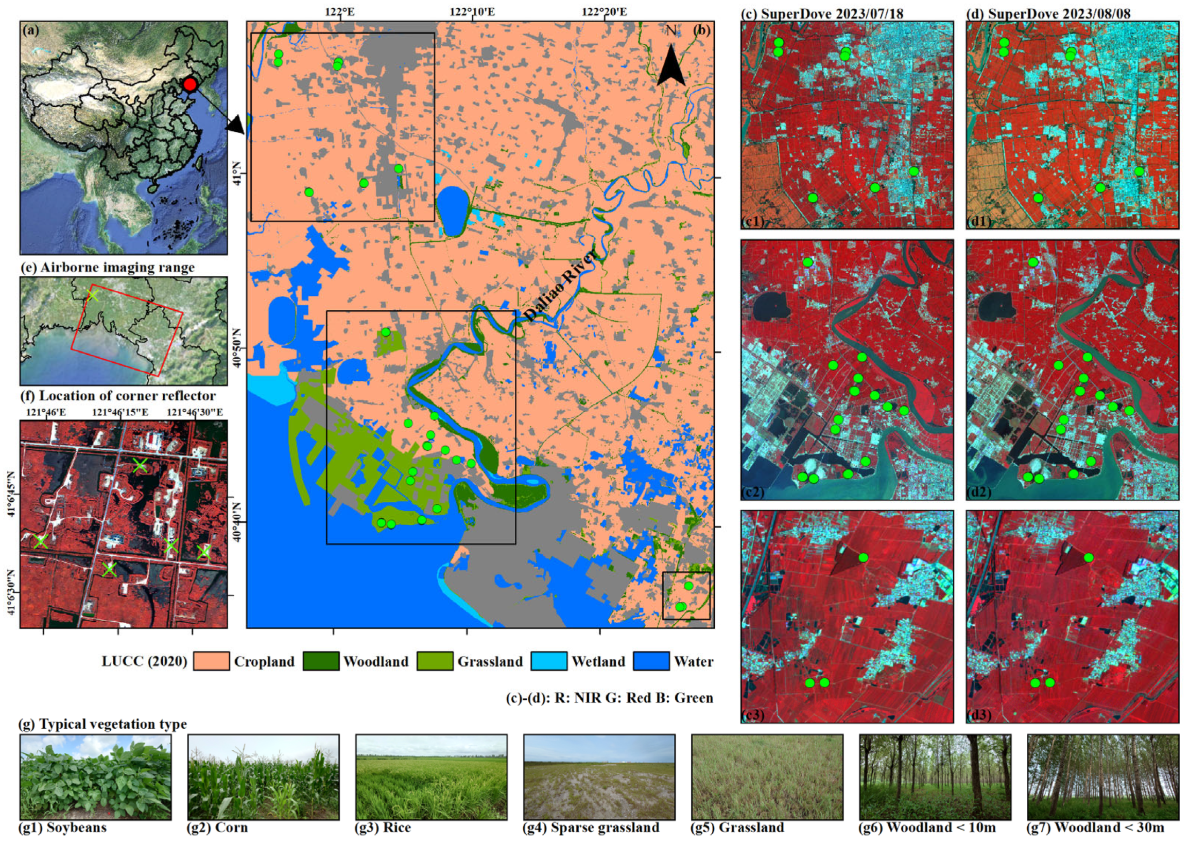
2.1. Liao River Basin

The study area lies in the central region of the Liao River Delta, at the mouth of the Liao River (Figure 1a). The terrain in this area is flat, with abundant water and no mountains, and it is the northernmost coastline in China. The Liao River and Daliao River run through the experimental area from north to south. The sampling teams, consisting of researchers from Wuhan University, China University of Mining and Technology (Xuzhou), Jiangsu Normal University, China University of Geosciences (Wuhan), and Hebei Normal University, selected three central sampling regions (Figure 1b) at the expected flight zone center on the airborne platform (Xinzhou-60), taking into account factors such as road accessibility, personnel allocation, surface cover types, flight path, airspace control, and the efficiency of synchronized observations. The sampling activity took place from 21 July 2023 to 5 August 2023 (Figure 1c,d). Based on the typical surface cover types in the study area, the sampling zones included 38 plots, including farmland (corn and soybeans), grassland, low woodland, and tall woodland (Figure 1e–g). Since the AMFSEX experiment was conducted for high-resolution airborne SAR data, each sample zone or plot was arranged with 6 to 16 sampling points, depending on the actual plot size, with sampling points spaced more than 3 m apart. The sampling process involved simultaneous surveys and sampling of both vegetation and soil, including vegetation types, phenological stages, growth status, leaf area index (LAI), multi-layer and profile SM (0–50 cm), soil physical parameters, and soil geometric parameters.

2.2. Xinzhou-60 Airborne Observation Platform

The multi-frequency quad-polarization (quad-pol) SAR data was sourced from the Xinzhu-60 platform of the Aerospace Information Research Institute, Chinese Academy of Sciences (AIR-CAS), which is capable of synchronized high-resolution SAR, hyperspectral, and multispectral observations. In the AMFSEX experiment, five corner reflectors (with right-angle sides of 1.4 m and 0.7 m) were placed along the flight path for SAR data radiometric calibration (Figure 1e,f). The raw data underwent a series of processing steps, including two-dimensional imaging, radiometric calibration, polarization calibration, conversion from single look complex images to backscattering coefficients, and geocoding, ultimately producing quad-pol SAR backscattering coefficients at five frequencies (Ka-, X-, C-, S-, L-band) with a spatial resolution of 0.3–1.0 m (Figure 2 and

Table 1. Parameter information of the remote sensing images.

Remote Sensing Imaging System	Imaging Band	Wavelength	Spatial Resolution
Xinzhou-60	Ka-band	1.0 cm	0.3 m
	X-band	3.1 cm	0.5 m
	C-band	5.6 cm
	S-band	10.0 cm	1.0 m
	L-band	24.0 cm
SuperDove	Coast blue	431–452 nm	3.0 m
	Blue	465–515 nm
	Green I	513–549 nm
	Green II	547–583 nm
	Yellow	600–620 nm
	Red	650–680 nm
	Red edge	697–713 nm
	NIR	845–885 nm

), including horizontal–horizontal (HH), horizontal–vertical (HV), vertical–horizontal (VH), and vertical–vertical (VV) polarization. A fourth-order polynomial fitting was used to obtain the antenna pattern for relative radiometric calibration. Absolute radiometric calibration coefficients were then calculated based on the theoretical radar cross section (RCS) of the corner reflectors and the RCS extracted from the SAR images. All images were subjected to both relative and absolute radiometric calibration. The polarization calibration was performed using the Whitt calibration algorithm, using the polarization calibration parameters extracted from the “three-face angle + 0° two-face angle + 45° two-face angle” setup (transmission distortion matrix, reception distortion matrix, absolute gain). The polarization calibration coefficients were then used for the polarization correction processing. The absolute radiometric accuracy is better than 2.5 dB, the relative radiometric accuracy is better than 1.0 dB, the polarization isolation is better than 25 dB, the amplitude imbalance is better than 1 dB (1σ), and the phase imbalance is better than 5 dB (1σ) [59].

2.3. SuperDove Optical Satellite Data

The SuperDove multispectral satellite data was selected as optical remote sensing data sources for characterizing vegetation growth conditions at the field scale in vegetation cover areas. After undergoing orthorectification, radiometric correction, atmospheric correction, and precise geometric correction, surface true reflectance images were obtained, including six visible bands (coast blue, blue, green I, green II, yellow, and red), one red-edge band, and one near-infrared (NIR) band. The spatial resolution of the SuperDove data is 3.0 m (Table 1).

2.4. Field Sampling Experiment

2.4.1. Vegetation Parameter Sampling

The ground vegetation types in the AMFSEX sampling activity primarily included rice, corn, soybeans, grassland (saltwort, reed), and woodland (birch forest and maple-leaf forest). Since the underlying surface of the rice fields was mainly water, rice was not considered a typical vegetation type for the observation experiment. The sampling team used a portable LAI measurement device (LAI2200) to measure the LAI of each sampling plot. Due to the limited sampling time, only one soil sampling point per plot was measured for the LAI. To reduce observational errors, each sampling point was measured repeatedly, and the mean of five measurements was taken as the final true LAI value. As shown in Figure 1g and

Table 2. Vegetation parameter information of sampling plots.

Sampling Plots	Sampling Phase	Land Cover Type	Vegetation Height	Measured LAI	Airborne SAR Data	Optical Data
ROI-7	24 July 2023	Corn	220–240 cm	3.2–4.2	Route16/24	18 July 2023–19 July 2023 (SuperDove)
ROI-8		Corn	220–250 cm	3.9–6.5
ROI-9		Corn	220–260 cm	3.9–5.4
ROI-10	25 July 2023	Corn	200–210 cm	3.2–4.4	Route27/28/31
ROI-11		Grassland	15–50 cm	0.4–0.6
ROI-12		Woodland (Maple-leaf Forest)	700–1070 cm	3.3–4.0
ROI-13	26 July 2023	Corn	250–260 cm	3.6–4.4	Route15/29/30
ROI-14		Corn	260–270 cm	3.5–5.3
ROI-15		Corn	270–280 cm	3.5–5.3
ROI-16		Soybeans	100–120 cm	6.3–8.3
ROI-17	27 July 2023	Soybeans	100–110 cm	6.3–8.3	Route15
ROI-18		Corn	250–260 cm	1.5–2.0
ROI-19		Soybeans	105–110 cm	5.0–6.3
ROI-20		Corn	205–210 cm	1.7–2.0
ROI-21 (11)	30 July 2023	Grassland	15–50 cm	0.4–0.6	Route30/31
ROI-22 (10)		Corn	200–210 cm	3.2–4.4
ROI-23		Corn	200–220 cm	3.0–4.5
ROI-24 (14)		Corn	260–270 cm	3.5–5.3
ROI-25 (15)		Corn	270–280 cm	3.5–5.3
ROI-26	31 July 2023	Woodland (Birch Forest)	1200–1300 cm	2.3–4.0	Route20/26
ROI-27		Woodland (Birch Forest)	1200–1300 cm	2.6–4.6
ROI-28		Corn	210–220 cm	2.3–3.8
ROI-29		Corn	220–240 cm	3.5–5.4
ROI-30	2 August 2023	Corn	220–240 cm	2.0–3.2	Route12/13/14	8 August 2023 (SuperDove)
ROI-31 (5)		Grassland	15–130 cm	1.4–3.0
ROI-32 (5)		Grassland	15–130 cm	2.0–2.4
ROI-33	4 August 2023	Grassland	90–100 cm	1.6–2.0
ROI-34		Corn	240–250 cm	3.1–3.6
ROI-35		Woodland (Maple-leaf Forest)	340–360 cm	2.7–3.0
ROI-36		Woodland (Birch Forest)	2400–2500 cm	2.6–30
ROI-37 (5)	5 August 2023	Grassland	15–130 cm	1.4–3.0	Route9/10/11
ROI-38		Grassland	5–10 cm	0.1–0.3

, the phenological stages of different crop types were generally consistent. A total of 17 corn sampling plots were surveyed, and the phenological stage was mainly in the tasseling and flowering periods, with vegetation height generally exceeding 200 cm and moderate to high vegetation cover (measured LAI > 3.5). It should be noted that a small number of corn plots had a weed-dominated underlying surface. Due to dense planting and field management, the growth of the soybeans was good (three sampling plots), with the plants in the flowering stage, a height exceeding 100 cm, and high vegetation cover (LAI > 6). The vegetation coverage in the grassland plots (seven sampling plots) was more complex. Due to the special geographic environment, the grassland in the wetland areas of the experimental region was often mixed with vegetation such as saltwort, reed, and foxtail grass, but the vegetation cover was relatively low (LAI < 2.5). The vegetation cover in the woodland plots (five sampling plots) was even more complex, with low shrubs and grassland in the underlying surface. However, due to the low density of trees, the vegetation cover was moderate (LAI < 4.5).

2.4.2. Soil Parameter Sampling

The sampling team measured the SSM (0–5 cm deep depth) using a handheld SM instrument (ML3) based on the frequency domain reflectance principle. If there were obvious ridges, sampling was conducted along the direction of the ridges, with sampling points evenly distributed within the field (

Table 3. Soil sampling information and airborne imaging information for different plots.

Vegetation Type	Sampling Plot	Soil Sampling (0–5 cm)	Soil Sampling (0–50 cm)	Sampling Phase	Whether Imaging Is Effective?					Radar Incidence Angle
					Ka-Band	X-Band	C-Band	S-Band	L-Band
Corn	ROI-7	√	√	24 July 2023	√	√	√	√	√	47.13–47.35°
	ROI-8	√	√		√	√	√	√	√	45.18–45.36°
	ROI-9	√	√		√	√	√	√	√	45.08–45.17°
	ROI-10	√	√	25 July 2023	√	√	√	√	√	47.31–47.55°
	ROI-13	√	√	26 July 2023	√	√	√	√	√	40.60–40.74°
	ROI-14	√	√		√	√	√	√	√	46.14–46.16°
	ROI-15	√	√		√	√	√	√	√	46.03–46.05°
	ROI-18	√	√	27 July 2023	√	√	√	√	√	38.85–39.16°
	ROI-20	√	×		√	√	√	√	√	51.02–51.09°
	ROI-22	√	√	30 July 2023	√	√	√	√	√	47.29–47.56°
	ROI-23	√	√		√	√	√	√	√	44.48–45.12°
	ROI-24	√	√		√	√	√	√	√	46.14–46.17°
	ROI-25	√	√		√	√	√	√	√	46.02–46.05°
	ROI-28	√	√	31 July 2023	√	√	√	√	√	45.79–46.16°
	ROI-29	√	√		√	√	√	√	√	45.64–46.01°
	ROI-30	√	×	2 August 2023	√	√	√	√	√	41.97–43.24°
	ROI-34	√	√	4 August 2023	√	√	√	√	√	45.41–45.89°
Soybeans	ROI-16	√	√	26 July 2023	√	√	√	√	√	46.64–47.50°
	ROI-17	√	√	27 July 2023	√	√	√	√	√	41.14–41.80°
	ROI-19	√	√		√	√	√	√	√	50.99–51.03°
Grassland	ROI-11	√	√	25 July 2023	√	√	√	√	√	47.51–47.71°
	ROI-21	√	√	30 July 2023	√	√	√	√	√	47.46–47.71°
	ROI-31	√	×	2 August 2023	√	√	√	√	√	41.28–42.07°
	ROI-32	√	×		√	√	√	√	√	50.88–51.80°
	ROI-33	√	√	4 August 2023	√	√	√	√	√	52.04–52.73°
	ROI-37	√	√	5 August 2023	√	√	√	√	√	41.28–42.12°
	ROI-38	√	√		√	√	√	√	√	41.55–42.27°
Woodland	ROI-12	√	√	25 July 2023	√	√	√	√	√	50.11–50.40°
	ROI-26	√	√	31 July 2023	√	√	√	√	√	42.19–42.97°
	ROI-27	√	√		√	√	√	√	√	42.57–43.25°
	ROI-35	√	√	4 August 2023	√	√	√	√	√	44.58–44.84°
	ROI-36	√	√		√	√	√	√	√	47.76–47.99°

). Measurements were taken at the top, middle, and bottom of the ridges, and the average of these three measurements was used as the SM for that sampling point. Each sampling area had one surface soil sample taken to calibrate the SM instrument. Each sampling area or plot had a multi-layer and profile SM sampling point, where soil samples were collected manually using soil augers. The soil sampling depths included 0–3 cm (considered as 3 cm deep SM, SSM-3 cm), 0–5 cm (5 cm deep SM, SSM-5 cm), 5–15 cm (10 cm deep SM, NSSM-10 cm), 15–25 cm (20 cm deep SM, NSSM-20 cm), 25–35 cm (30 cm deep SM, NSSM-30 cm), 35–45 cm (40 cm deep SM, RZSM-40 cm), and 45–55 cm (50 cm deep SM, RZSM-50 cm). Soil from these depths was collected using the ring knife method to determine its bulk density. The samples were weighed immediately to minimize errors due to moisture evaporation. All soil samples were dried (at 105–110 °C for 24 h) at the Soil Science Research Center of the School of Urban and Environmental Sciences at Central China Normal University (CCNU). The volumetric SM (cm³/cm³) for each sampling point was obtained from the bulk density of each sample. The soil texture type composition (STT, including clay, sand, and silt proportion) and the soil organic matter (SOM) content of different soil depths were determined using the soil hydrometer method and the potassium dichromate oxidation-spectrophotometric method, respectively. Moreover, the sampling team measured the soil roughness (SR) of each plot using a customized pin board (1.2 m long). Measurements were taken perpendicular and parallel to the flight direction of the airborne platform, and photos were taken. Depending on the size of the plot, multiple measurements were taken at one sampling point to reduce uncertainty in the roughness measurements. Finally, the photos were digitized to obtain the root mean square height (s) and correlation length (l) of each sampling point. Sample truth data are detailed in the Supplementary Materials.

3. Methods

3.1. Technical Process

This study mainly explored the potential and uncertainty of estimating the multi-layer and profile SM under different vegetation types based on the high-resolution airborne multi-frequency quad-pol SAR data. First, the vegetation types, phenological stages, and growth conditions of the sampling points in the study area, as well as the measured soil parameters (multi-layer and profile SM, soil texture, etc.) were analyzed. Second, the “theoretical” penetration depth of the multi-frequency SAR data was analyzed based on the Dobson empirical model and the Hallikainen correction model. On this basis, the similarities and differences between the multispectral data and the multi-frequency SAR data in representing vegetation growth were analyzed. Using the water cloud model (WCM) with multi-polarization weighting and penetration depth weighting constraints, the estimation accuracy of the multi-layer and profile SM under different vegetation types using the multi-frequency SAR data (Ka-, X-, C-, S-, L-band) was analyzed. Finally, the multi-layer and profile SM were estimated synchronously using a multi-input multi-output regression model, and the estimation accuracy was compared with that of the scattering model.

3.2. Soil Moisture Estimation Model

3.2.1. Water Cloud Model

The scattering contribution of vegetation reduces the sensitivity of the SAR signals to the underlying SM, making it highly challenging to directly estimate SM from backscattering coefficients [20,60,61,62]. As SAR frequency increases, signal attenuation becomes more pronounced. Therefore, eliminating or minimizing the vegetation scattering contribution is key to accurately estimating the SM in vegetated areas. The WCM, based on radiative transfer theory, is relatively simple and practical for describing radar scattering mechanisms in low-growing vegetation [19,35,62,63,64,65,66]. This model assumes that the vegetation layer is composed of many uniformly distributed scattering particles of the same shape and size, and it neglects multiple scattering between vegetation and the soil surface. In this model, the total backscattering (${\sigma }_{pq}^{total}$) consists of direct scattering from the vegetation layer (${\sigma }_{pq}^{veg}$) and soil scattering attenuated bidirectionally through the vegetation (${\sigma }_{pq}^{soil}$). The basic form of the WCM is as follows:

$${\sigma }_{pq}^{total}={\sigma }_{pq}^{veg}+{\gamma }^2{\sigma }_{pq}^{soil}\times \left(\cos {\theta }_i\right)$$

(1)

$${\sigma }_{pq}^{veg}=A\times Veg\times \left(\cos {\theta }_i\right)\times \left(1-{\gamma }^2\right)$$

(2)

$${\gamma }^2=e^{-2B\times Veg\times \sec {\theta }_i}\approx 1-{\displaystyle \frac{2B\times Veg}{\cos {\theta }_i}} \left(Taylor \exp ansion\right)$$

(3)

In general, the exponential terms mentioned above are typically expanded using a multi-order Taylor series to transform the nonlinear problem into a linear one without compromising the final estimation accuracy [19,24]. In addition, there is a strong exponential relationship between the vegetation-corrected soil backscattering coefficients and the SM, which allows the use of a first-order Taylor series expansion to further refine the SM estimation formula, as follows [35,66]:

$${\sigma }_{pq}^{soil}=C\times \exp \left(SM\right)+D$$

(4)

$$S{M}_{pq}^{soil}=e^{{\displaystyle \frac{1}{C}}\times \left({\sigma }_{pq}^{soil}-D\right)}\approx 1+{\displaystyle \frac{1}{C}}\times \left({\displaystyle \frac{{\sigma }_{pq}^{total}-2AB\times Ve{g}^2}{1-2B\times Veg\times \sec {\theta }_i}}-D\right)$$

(5)

where ${\sigma }_{pq}^{tatal}$ is the total backscattering coefficient (in linear power) of a SAR pixel, ${\sigma }_{pq}^{veg}$ is the backscattering coefficient from the vegetation layer, ${\sigma }_{pq}^{soil}$ is the backscattering coefficient from the soil layer after bidirectional attenuation, ${\gamma }^2$ is the bidirectional attenuation factor, ${\theta }_i$ is the radar incidence angle of a SAR pixel, Veg represents the vegetation descriptors, and pq represents the radar polarization mode, which can be either co-polarization (HH and VV) or cross-polarization (HV and VH). The semi-empirical parameter A represents the backscattering coefficients of dense vegetation (related to vegetation types and growth status), and it approaches zero when the surface cover is bare soil. The semi-empirical coefficient B represents the attenuation coefficient, which quantifies the scattering effect of SM and vegetation on microwave radiation. The semi-empirical coefficient C reflects the sensitivity of the SAR signal to SM in bare soil areas (influenced by factors such as soil texture and SM). The semi-empirical coefficient D depends on the SAR system parameters (e.g., wavelength, polarization mode, and radar incidence angle).

The estimation of semi-empirical parameters in the WCM generally follows two approaches: one is to first derive the parameters for bare soil areas (C and D), followed by those for vegetated areas (A and B); the other is to solve all parameters simultaneously [19,66]. In this study, the latter approach was adopted, and the semi-empirical coefficients were fitted using the Levenberg–Marquardt (LM) global optimization least squares algorithm in combination with in situ SM [24,35,67]. Additionally, independent calibration is required for different polarizations and crop types to ensure the reliability and estimation accuracy of the SM modeling. Since this study aims to explore the potential and uncertainty of using the multi-frequency SAR data to estimate the multi-layer and profile SM, the optimization of the scattering model itself is beyond the scope of this study. Vegetation descriptors in the WCM model were represented using both optical and radar-based vegetation indices, including the normalized difference vegetation index (NDVI) and the cross-polarization ratio (CPR), as follows:

$$NDVI={\displaystyle \frac{{\rho }_{NIR}-{\rho }_{Red}}{{\rho }_{NIR}+{\rho }_{Red}}}$$

(6)

$$CP{R}_H={\sigma }_{HV}/{\sigma }_{HH}$$

(7)

$$CP{R}_V={\sigma }_{VH}/{\sigma }_{VV}$$

(8)

where ${\rho }_{red}$ and ${\rho }_{NIR}$ represent the surface true reflectance values of the red and NIR bands from the SuperDove images, respectively, ${\sigma }_{HH}$, ${\sigma }_{HV}$, ${\sigma }_{VH}$, and ${\sigma }_{VV}$ represent the backscattering coefficients under HH, HV, VH, and VV polarizations in linear power, CPR_H represents the CPR under the HH + HV mode, and CPR_V represents the CPR under the VV + VH mode.

There is currently no consensus on which polarization mode is most accurate for estimating SM under different vegetation conditions [62,63,68]. Generally, researchers believe that co-polarization (HH or VV) offers stronger vegetation penetration capability and is therefore more suitable for SM estimation. However, recent studies have shown that cross-polarization (HV or VH) also has the potential to represent SM in vegetated areas [10,68]. In this study, multi-polarization joint estimation combined with adaptive weighted constraints was employed to improve the estimation accuracy of SM in the WCM. The weights for different polarization modes were represented by their scattering power. According to the results of this study, the adaptive weighting approach effectively reduces outliers in the estimation results and significantly lowers the SM estimation errors. For the quad-pol SAR data, the final expression for estimating SM is as follows:

$$S{M}_{f_i-band}^{quad-pol}=W_{HH}\times S{M}_{HH}+W_{HV or VH}\times S{M}_{HV or VH}+W_{VV}\times S{M}_{VV}$$

(9)

$$\begin{array}{l}{W}_{HH}={\displaystyle \frac{{\sigma }_{f_i-band,HH}}{{\sigma }_{f_i-band,HH}+{\sigma }_{f_i-band,HV or VH}+{\sigma }_{f_i-band,VV}}}\\ W_{HV or VH}={\displaystyle \frac{{\sigma }_{f_i-band,HV or VH}}{{\sigma }_{f_i-band,HH}+{\sigma }_{f_i-band,HV or VH}+{\sigma }_{f_i-band,VV}}}\\ W_{VV}={\displaystyle \frac{{\sigma }_{f_i-band,VV}}{{\sigma }_{f_i-band,HH}+{\sigma }_{f_i-band,HV or VH}+{\sigma }_{f_i-band,VV}}}\end{array}$$

(10)

where $S{M}_{f_i-band}^{quad-pol}$ represents the weighted SM estimation values based on the quad-pol SAR data at different frequencies (Ka-, X-, C-, S-, L-band), $S{M}_{HH}$, $S{M}_{HV or VH}$, and $S{M}_{VV}$ represent the SM estimation values under HH, HV (or VH), and VV polarizations, respectively, and $W_{HH}$, $W_{HV or VH}$, and $W_{VV}$ represent the corresponding weights under HH, HV (or VH), and VV polarizations, respectively.

For the multi-frequency SAR data (Ka-, X-, C-, S-, and L-band), the “vegetation–soil” penetration capability varies due to differences in radar frequency. Therefore, joint modeling using the multi-frequency SAR data can improve the estimation accuracy of the multi-layer and profile SM. Assuming that the influence of vegetation scattering can be effectively removed through vegetation sensitivity constraints and multi-polarization inversion constraints, SM estimation values ($S{M}_{f_i-band}$) based on the quad-pol SAR data at different frequencies can be obtained. However, their respective effective soil penetration depths remain unknown. For single-frequency SAR signals, the effective soil penetration depth (d_penetration) is defined as the propagation distance in a lossy medium where the incident wave power attenuates to 1/e of its initial value [69]. After removing the vegetation scattering contribution, SAR signals at different frequencies still experience attenuation in the soil, meaning that the signal weakens as the soil depth increases. In this study, the “theoretical” soil penetration depths ($d_{f_i-band}$) of the multi-frequency SAR data were analyzed based on the Dobson dielectric mixing empirical model and the Hallikainen correction model [70,71]. These depths are related to SM content, STT, radar frequency, and radar incidence angle. Therefore, the effective penetration depth of the SAR data at different frequencies can be considered a function of radar wavelength and soil dielectric constant, as follows:

$$\begin{array}{rr}\epsilon \left({\epsilon }^{\prime },{\epsilon }^{″}\right)=& \left(a_0+a_1{f}_{sand}+a_2{f}_{clay}\right)+\left(b_0+b_1{f}_{sand}+b_2{f}_{clay}\right)\times m_v\hfill \\ \hfill +& \left(c_0+c_1{f}_{sand}+c_2{f}_{clay}\right)\times {m_v}^2\hfill \end{array}$$

(11)

$$d_{f_i-band}=f\left(m_v,STT,v,\theta \right)={\displaystyle \frac{\sqrt{2}\lambda }{2\pi \sqrt{{\epsilon }^{\prime }-{\sin }^2{\theta }_i}\sqrt{{\left(1+\frac{{\epsilon }^{″2}}{{\left({\epsilon }^{\prime }-{\sin }^2{\theta }_i\right)}^2}\right)}^{0.5}-1}}}$$

(12)

where ${\epsilon }^{\prime }$ and ${\epsilon }^{″}$ represent the real and imaginary parts of the soil dielectric constant, respectively. The real part characterizes the refraction and reflection of electromagnetic waves at the interface between two different media, while the imaginary part represents the attenuation of incident electromagnetic waves in the soil (due to absorption and conversion). The values for a₀–a₂, b₀–b₂, and c₀–c₂ are empirical polynomial fitting coefficients related to radar frequency (ν) [70,71] and $d_{f_i-band}$ represents the effective soil penetration depth of the SAR data at different frequencies, which is influenced by the SM content (mᵥ), soil texture composition (STT; f_clay, f_sand, and f_silt), radar wavelength (λ), and radar incidence angle (θᵢ).

Under the same radar system parameters and surface conditions (i.e., when the multi-frequency SAR data are acquired simultaneously), the penetration depth of the SAR data is generally positively correlated with the radar wavelength and negatively correlated with the radar frequency. Moreover, the differences in the penetration depth are linearly related to differences in the radar frequency. According to the in situ multi-layer and profile SM at each sampling point, the STT does not exhibit significant stratification. Therefore, the weighted average expression for the multi-layer and profile SM (0–50 cm depth) based on the five-frequency SAR data and their respective penetration depths is as follows:

$$S{M}_{i-cm}={\displaystyle \sum \left(d_{f_i-band}^{\prime }\times S{M}_{f_i-band}+d_r\right)}$$

(13)

where $S{M}_{i-cm}$ represents the SM estimation values at different depths, weighted by penetration depth, including 3 cm, 5 cm, 10 cm, 20 cm, 30 cm, 40 cm, and 50 cm, $S{M}_{f_i-band}$ represents the SM estimation values derived from the five-frequency quad-pol SAR data using the WCM (assuming each frequency can penetrate to different depths), $d_{f_i-band}^{\prime }$ represents the penetration depth weights for the five frequencies, which are related to the theoretical penetration depth and radar frequency, and $d_r$ represents the residual term of the model, which are related to SAR frequency and effective penetration depth. These weights can be fitted using in situ SM at different depths and the LM global optimization least squares algorithm.

3.2.2. Gaussian Process Regression Model

Gaussian Process Regression (GPR) is a non-parametric regression algorithm designed to model the underlying relationship between input variables and output data [72,73]. It is based on the concept of a Gaussian process, which allows for effective modeling of function uncertainty. GPR uses observed data to make predictions for new data points and features highly flexible kernel functions that can adapt to functional relationships across different data types. The GPR algorithm not only captures complex relationships between variables but provides valuable uncertainty information for predictions. Existing studies have shown that GPR outperforms ensemble learning regression algorithms in SM modeling [74,75]. This study evaluated the SSM estimation accuracy (0–5 cm) using the multi-frequency SAR data, and further explored the upper limit of estimation performance when incorporating multispectral data, soil physical parameters (STT and SOM), and soil geometric parameters (SR). In addition, multi-layer and profile SM (0–50 cm) was treated as a multi-input multi-output regression problem and compared with the results derived from the scattering model (WCM). The hyperparameters of the regression models were optimized iteratively using a Bayesian optimization algorithm [76]. The detailed procedure can be found in the previously published studies [74,75].

3.3. Model Validation Strategies and Accuracy Indices

3.3.1. Model Validation Strategies

Considering the limited number of in situ measurements, the number of SSM samples was fewer than 400, and the number of multi-layer and profile SM samples was fewer than 40. In this study, the measured SSM data were categorized by crop types and then randomly divided into two parts: half of the data (Part A) were randomly selected for model construction, i.e., for calibrating the semi-empirical coefficients of the WCM or for training the regression model, while the other half (Part B) were used for accuracy evaluation. The process was then reversed, with Part B used for modeling and Part A for validation. This random data-splitting strategy helps reduce the adverse effects of field variability (e.g., phenological stages, soil texture, and topography) on SM modeling and provides a feasible approach for optimizing and evaluating SM estimation models [77]. It should be noted that, due to the limited number of multi-layer and profile SM sampling points, this study employed a leave-one-out cross-validation approach to construct multi-frequency SAR-based models for the multi-layer and profile SM estimation [78,79,80,81]. Separate calibrations and model validations were conducted for different vegetation types (e.g., cropland, grassland, and woodland).

3.3.2. Accuracy Indices

The SM estimation models were evaluated using several accuracy evaluation metrics, including the Pearson correlation coefficient (R), mean absolute error (MAE), and root mean square error (RMSE). The corresponding expressions are as follows:

$$R={\displaystyle \frac{Cov\left(X,Y\right)}{\sqrt{Var\left(X\right)Var\left(Y\right)}}}$$

(14)

$$MAE={\displaystyle \frac{1}{N}}\times {\displaystyle \sum _{i=1}^N\left|X_{model,i}-X_{obs,i}\right|}$$

(15)

$$RMSE=\sqrt{{\displaystyle \frac{{\displaystyle {\sum }_{i=1}^n{\left(X_{model,i}-X_{obs,i}\right)}^2}}{n}}}$$

(16)

where $Cov\left(X,Y\right)$ represents the covariance between X and Y, while $Var\left(X\right)$ and $Var\left(Y\right)$ represent the variances of X and Y, respectively, while $X_{obs,i}$ and $X_{model,i}$ correspond to the observed and estimated values of the i-th sample, and N is the total number of samples.

4. Results and Discussions

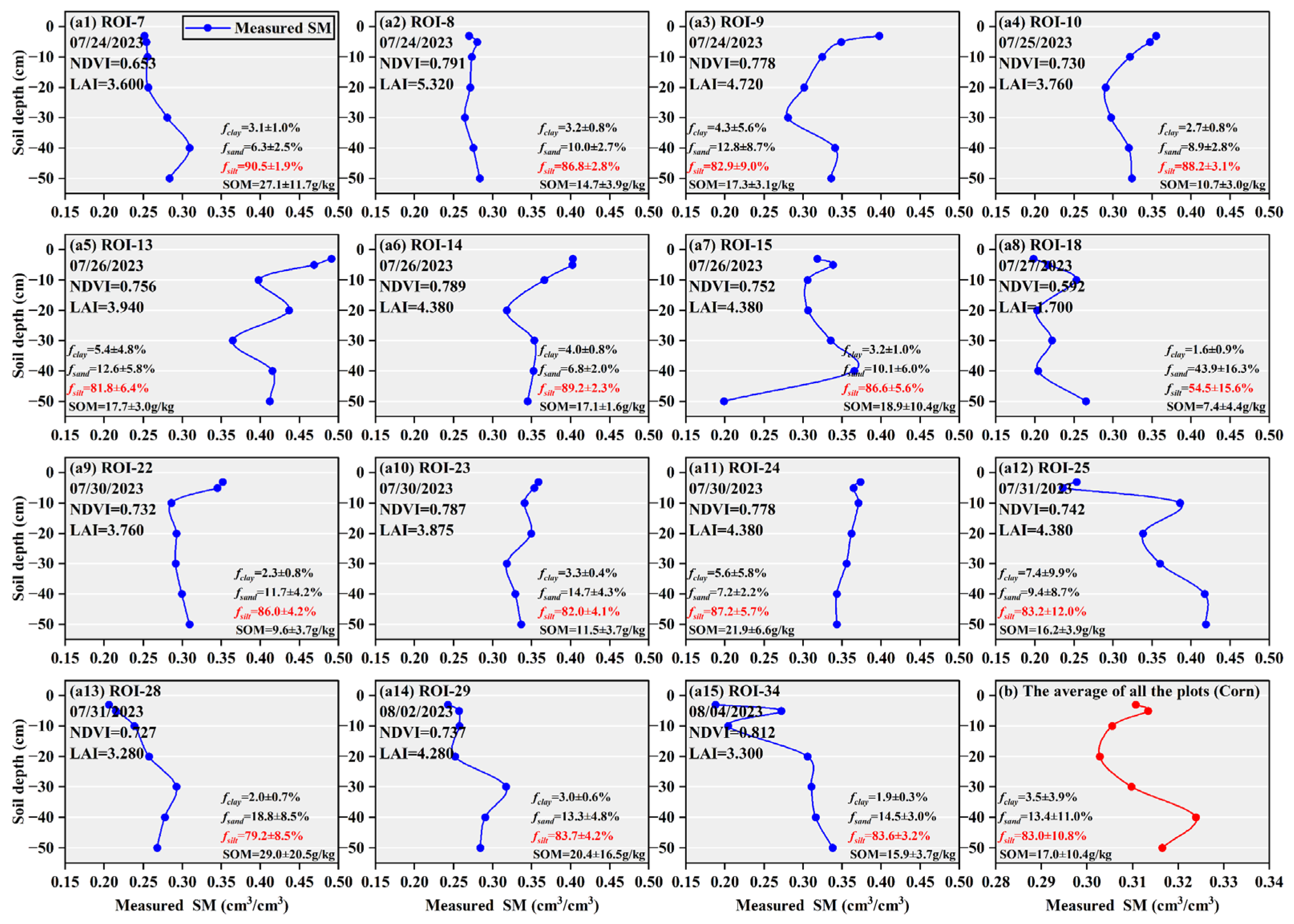
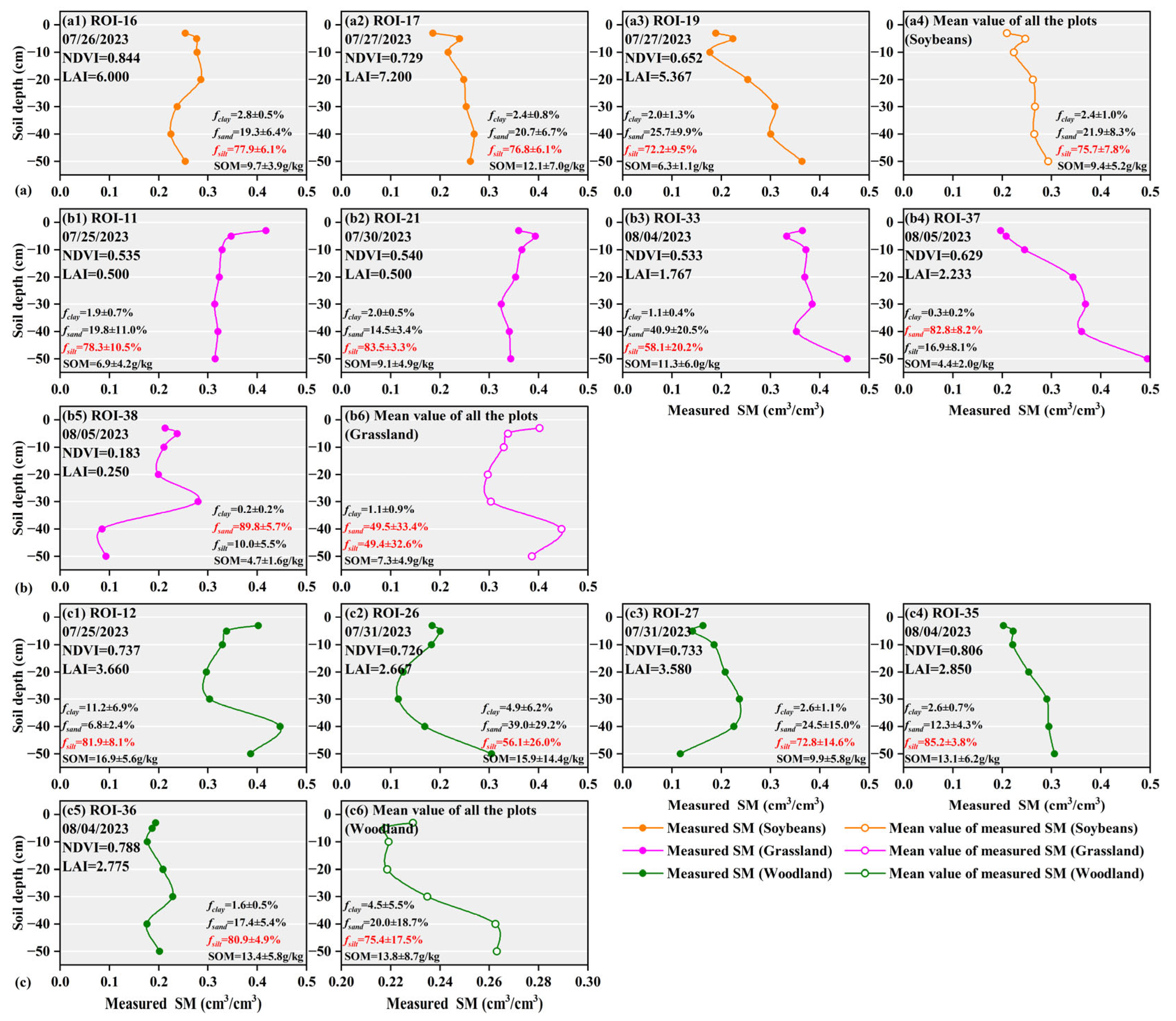
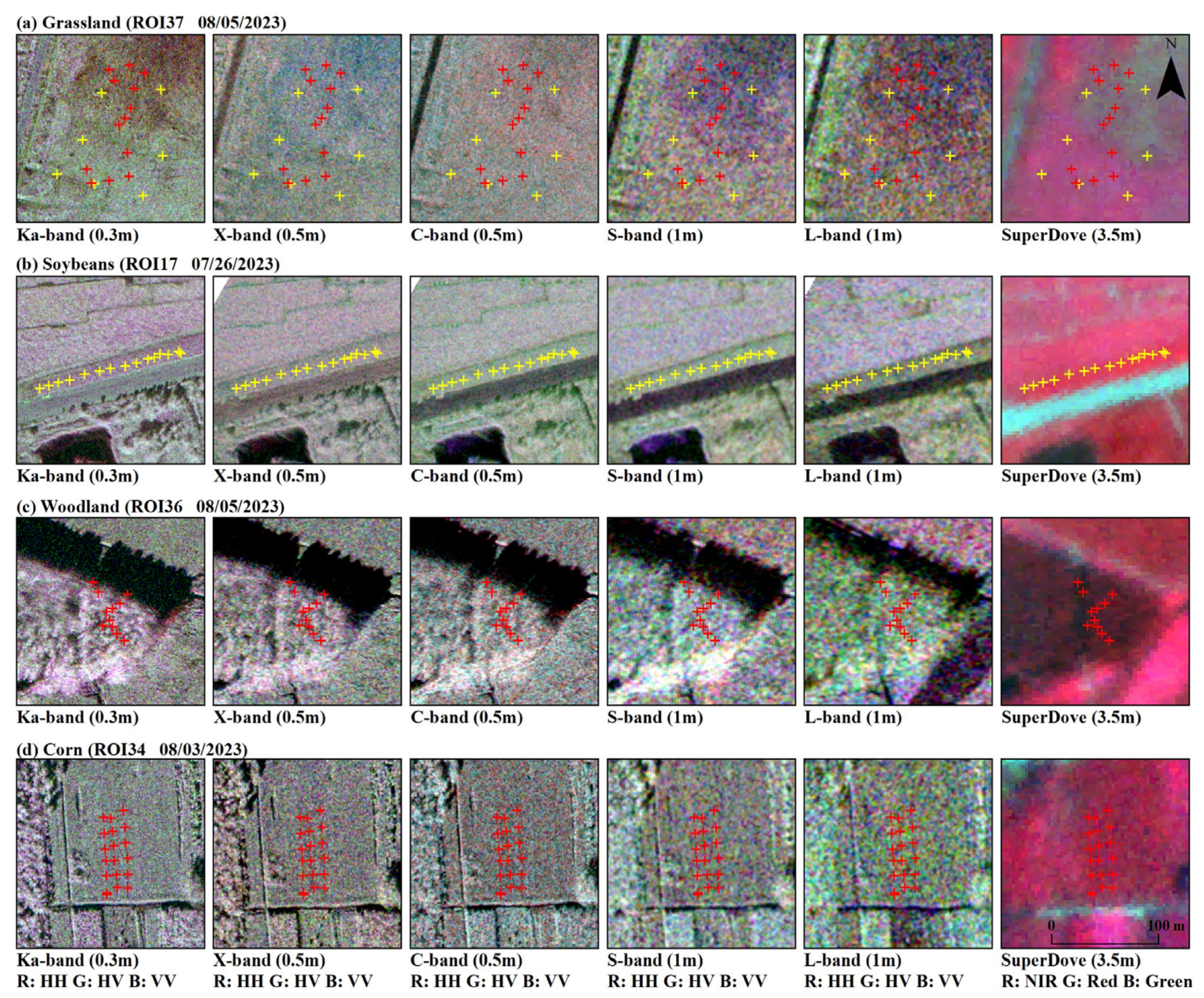
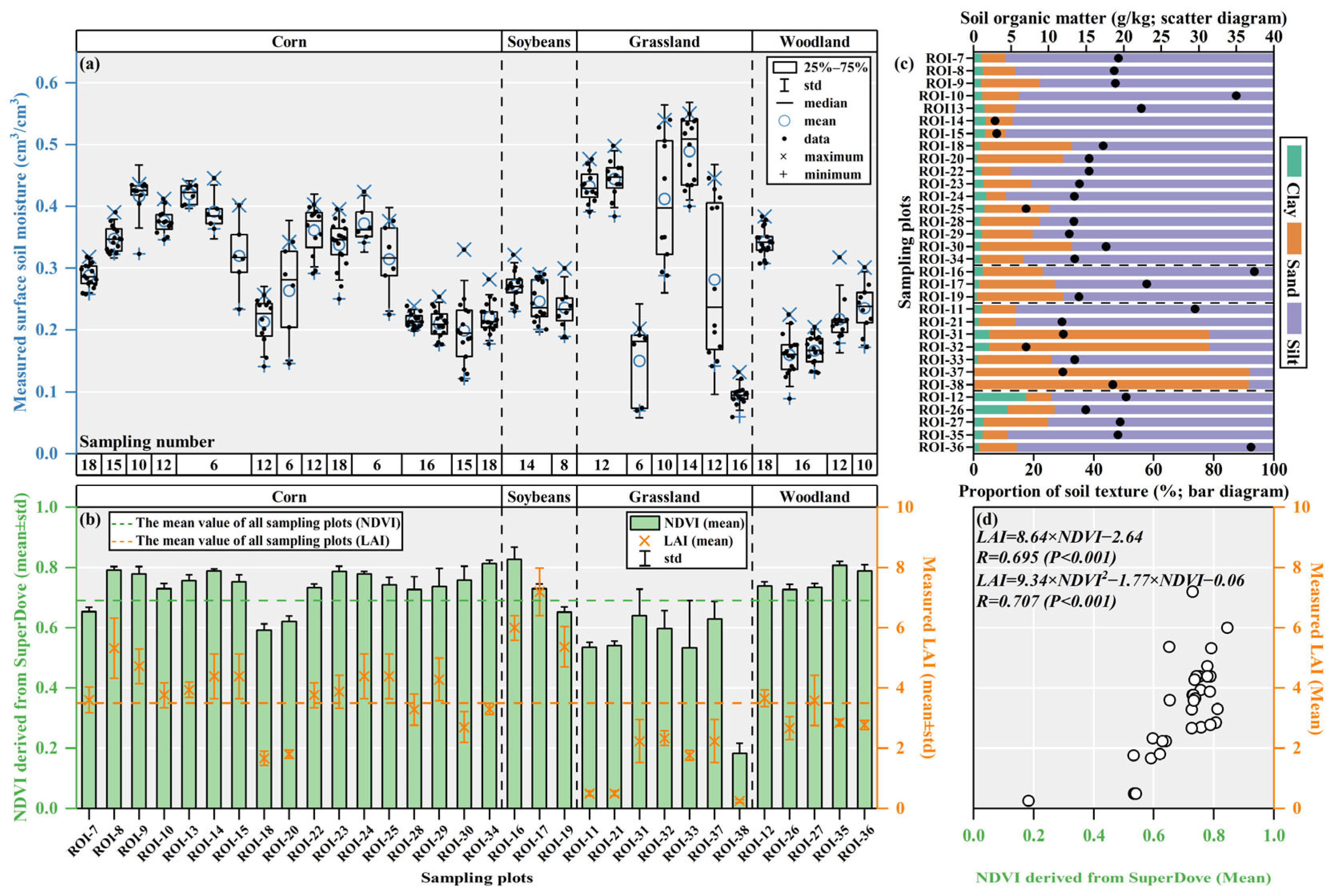
4.1. Analysis of Vegetation and Soil Parameters in the Sampling Plots

As shown in Figure 3, the STT in the study area is primarily silty soil, with moderate SOM (SOM_mean±std = 18.4 ± 9.1 g/kg). There are significant differences in the measured SSM (0–5 cm) across the different sampling plots. The grassland sampling areas, which consist of seven plots, are mainly located in the wetland areas of the experimental region. These plots have sandy soils as the dominant STT and a generally high SM content (SM_mean±std = 0.333 ± 0.162 cm³/cm³), with considerable variation in SM within the same sampling plot. The corn and soybean sampling areas consist of 17 plots and 3 plots, respectively, with moderate SM content (SM_mean±std = 0.288 ± 0.077 cm³/cm³). The woodland sampling areas consist of five plots, with relatively low SM content (SM_mean±std = 0.227 ± 0.078 cm³/cm³). Due to the peak summer season, vegetation growth in the experimental area is lush, with an average NDVI of 0.678 (±0.143) and an average measured LAI of 3.357 (±1.547). There is a good correlation between the NDVI derived from the SuperDove images and the measured LAI (R = 0.695), with grassland showing lower vegetation cover and corn, soybean, and woodland areas showing higher vegetation cover.

As shown in

Table A1. The measured SM statistical values of sampling plots with different vegetation types.

Vegetation Type	Soil Depth	Mean (cm3/cm3)	Standard Deviation	Coefficient of Variation
Entirety	3 cm	0.285	0.092	0.322
	5 cm	0.287	0.076	0.265
	10 cm	0.281	0.069	0.244
	20 cm	0.286	0.063	0.222
	30 cm	0.307	0.090	0.293
	40 cm	0.301	0.078	0.259
	50 cm	0.316	0.105	0.332
Corn	3 cm	0.311	0.086	0.276
	5 cm	0.313	0.071	0.225
	10 cm	0.306	0.057	0.186
	20 cm	0.303	0.054	0.177
	30 cm	0.310	0.039	0.126
	40 cm	0.324	0.052	0.162
	50 cm	0.317	0.055	0.172
Soybeans	3 cm	0.209	0.031	0.149
	5 cm	0.247	0.022	0.090
	10 cm	0.224	0.041	0.185
	20 cm	0.263	0.016	0.062
	30 cm	0.267	0.030	0.114
	40 cm	0.265	0.031	0.117
	50 cm	0.293	0.050	0.171
Grassland	3 cm	0.310	0.089	0.286
	5 cm	0.304	0.070	0.230
	10 cm	0.304	0.065	0.214
	20 cm	0.318	0.061	0.192
	30 cm	0.394	0.148	0.375
	40 cm	0.292	0.104	0.357
	50 cm	0.380	0.187	0.494
Woodland	3 cm	0.229	0.088	0.382
	5 cm	0.218	0.065	0.301
	10 cm	0.219	0.057	0.261
	20 cm	0.219	0.057	0.261
	30 cm	0.235	0.066	0.283
	40 cm	0.262	0.102	0.390
	50 cm	0.263	0.094	0.356

Note: Bold indicates that the SM at this depth has the least variability.

and Figure A1 and Figure A2 in Appendix A, there are significant differences in the multi-layer and profile SM (0–50 cm) across the different sampling plots. For different plots, the differences in the STT at various depths are small, but the SOM content generally decreases with increasing soil depth. For the corn sampling points (15 plots), the multi-layer STT is primarily silty soil (83.0 ± 12.0%), with relatively high SOM (17.0 ± 10.4 g/kg). The mean SM at each sampling point decreases with increasing soil depth, then increases, and finally decreases again. The soybean sampling points have relatively low SOM (9.4 ± 5.2 g/kg), and the mean SM increases almost linearly with increasing soil depth. The grassland sampling points have a mix of silty and sandy soils, with low SOM content (7.3 ± 4.9 g/kg), and the mean SM decreases with increasing depth, then increases again. The woodland sampling points have moderate SOM (13.8 ± 8.7 g/kg), and due to significant rainwater interception, the mean SM remains relatively constant at deeper soil layers before steadily increasing, exhibiting a notable time delay effect.

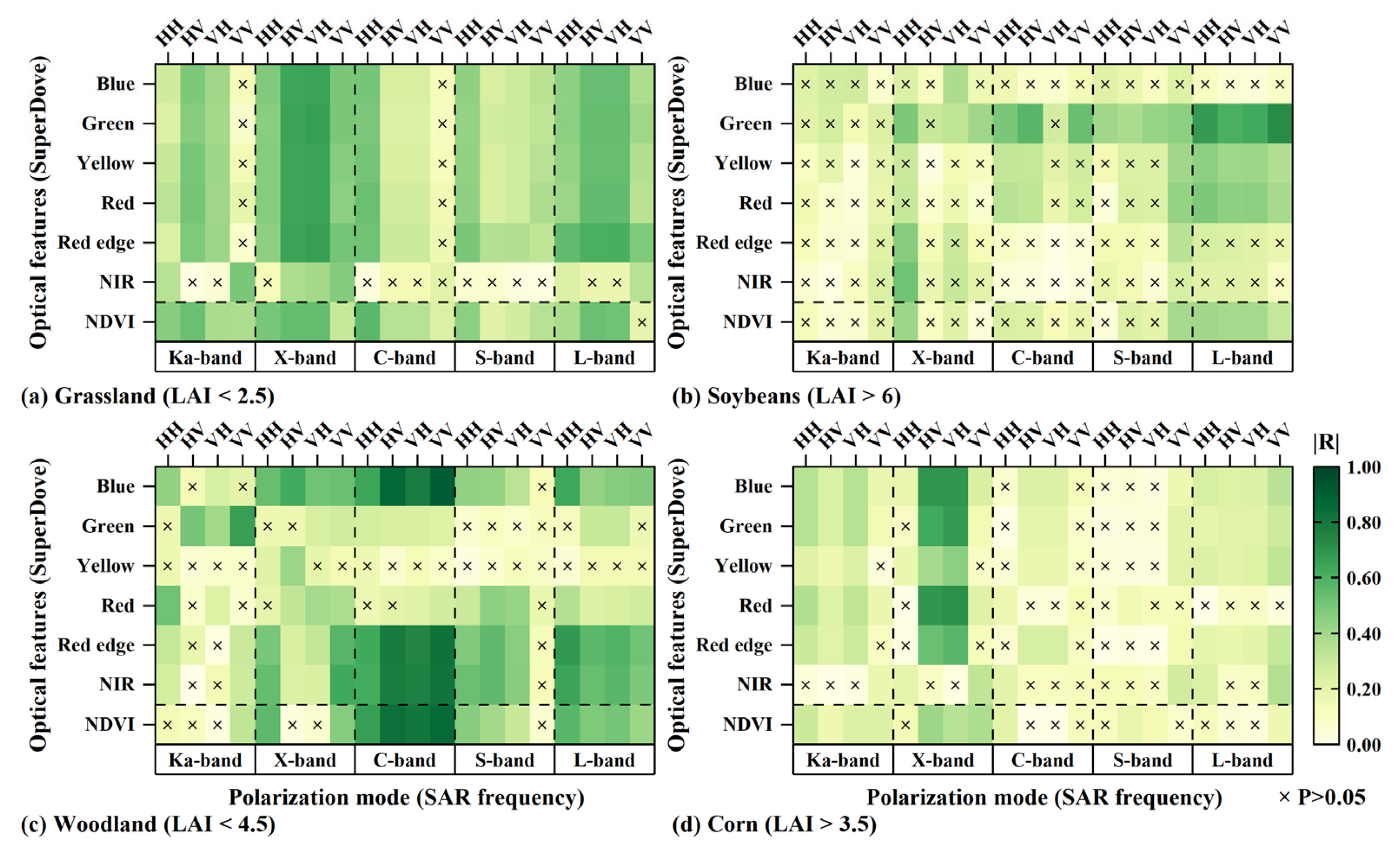
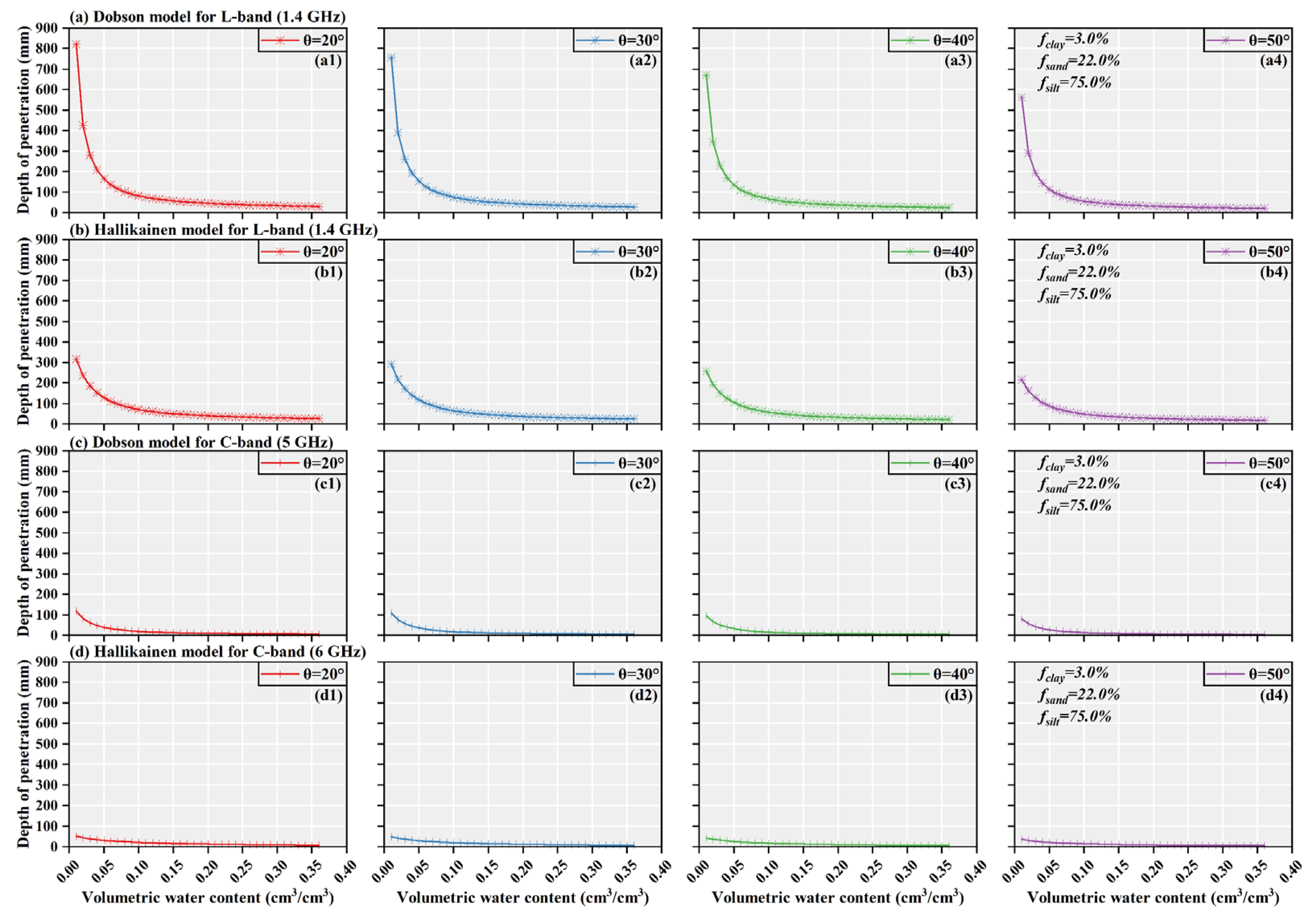
4.2. Theoretical Analysis and Simulation Experiment of Soil Penetration Using the Multi-Frequency SAR Data

This study employed the Dobson empirical model and the Hallikainen modified model to simulate the relationship between the soil dielectric constant and microwave signal penetration depth at different frequencies, including the L-band and C-band SAR data. Based on the soil properties of the joint observation experimental area, different radar incidence angles (20°, 30°, 40°, 50°) and the STT compositions (f_clay = 3.0%, f_sand = 22.0%, f_silt = 75.0%) were set. As shown in Figure 4, the simulation results indicate that, as the SM content and radar frequency increase, the penetration capability of SAR signals into the soil gradually weakens. Under extremely low SM conditions (less than 0.050 cm³/cm³), the penetration capability of L-band SAR signals is approximately 4–7 times that of the C-band. When the SM content exceeds 0.150 cm³/cm³, the penetration depth of the L-band is less than 10 cm, while that of the C-band is only 0–5 cm. Compared with the Dobson model, the Hallikainen model is more sensitive to the STT composition. For the same model and radar frequency, a lower radar incidence angle results in a greater soil penetration depth of the SAR signals [69,82]. Overall, as SM content, radar incidence angle, and SAR frequency increase, the soil penetration depth of the SAR signals decreases. The measured SSM in different sampling plots of the study area ranges from 0.095 cm³/cm³ to 0.489 cm³/cm³, indicating that the theoretical penetration depth of the multi-frequency SAR data varies across sampling plots. Additionally, the SM in the vertical profile is not uniform, further increasing the complexity of evaluating the SAR signal penetration performance. However, neither the Dobson nor the Hallikainen model accounts for the effects of SOM and SR on radar penetration depth [69,82]. The above analysis demonstrates the potential for retrieving the multi-layer and profile SM using the multi-frequency SAR data, which requires further analysis and validation in combination with the measured sampling data.

4.3. Estimation Modeling and Validation of Multi-Layer and Profile Soil Moisture Based on the Multi-Frequency SAR Data

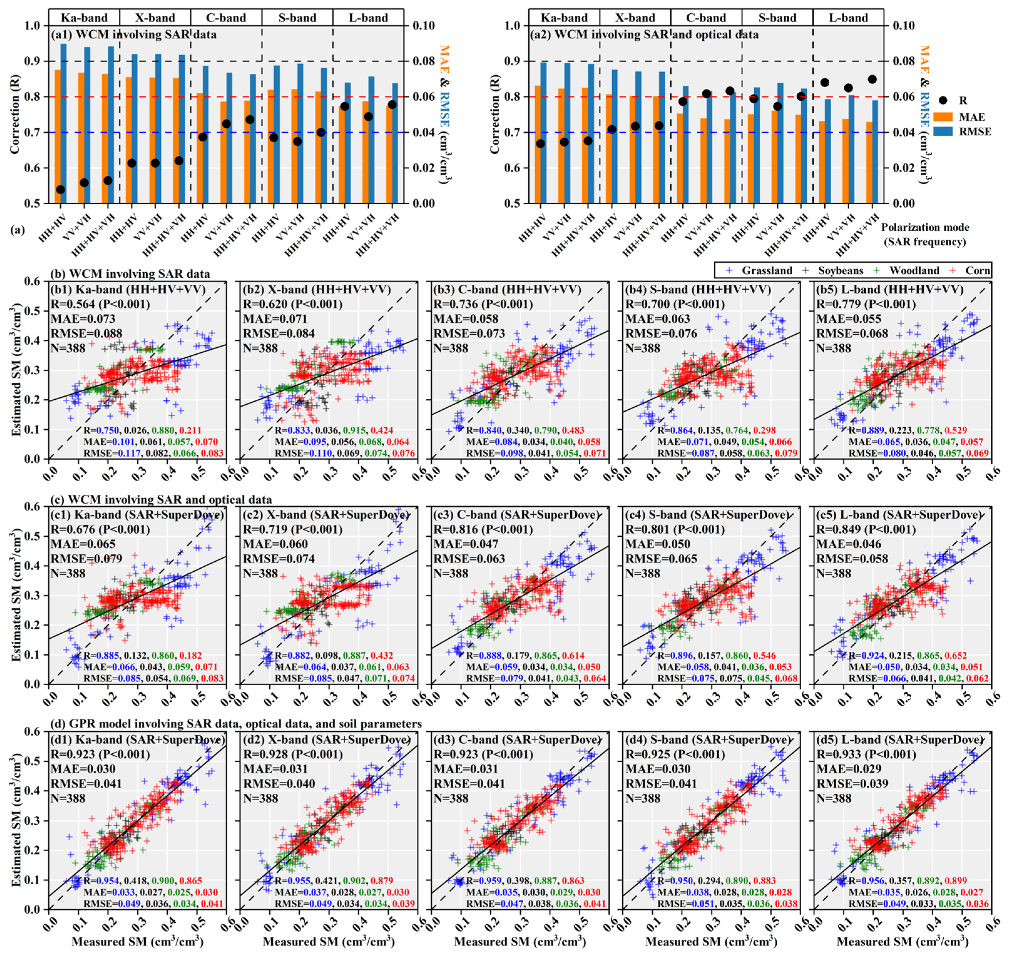
4.3.1. Evaluation of Surface Soil Moisture Estimation Accuracy Based on the Scattering Model and the Regression Model

As shown in Figure 5 and

Table A2. Estimation accuracy of SSM (0–5 cm) for different vegetation types based on the scattering model and the regression model.

Estimation Model	Polarization Mode	Accuracy Indices	SAR Frequency
			Ka-band	X-band	C-band	S-band	L-band
WCM1	HH+HV	R	0.539	0.614	0.687	0.685	0.773
		MAE	0.075	0.071	0.062	0.064	0.055
		RMSE	0.090	0.084	0.078	0.078	0.068
	VV+VH	R	0.559	0.614	0.724	0.675	0.744
		MAE	0.074	0.071	0.057	0.064	0.058
		RMSE	0.088	0.084	0.074	0.079	0.071
	HH+HV+VV	R	0.564	0.620	0.736	0.700	0.779
		MAE	0.073	0.071	0.058	0.063	0.055
		RMSE	0.088	0.084	0.073	0.076	0.068
WCM2	HH+HV	R	0.669	0.708	0.787	0.795	0.840
		MAE	0.066	0.061	0.051	0.050	0.046
		RMSE	0.079	0.075	0.066	0.065	0.059
	VV+VH	R	0.672	0.718	0.809	0.773	0.825
		MAE	0.065	0.061	0.045	0.052	0.047
		RMSE	0.079	0.074	0.063	0.068	0.061
	HH+HV+VV	R	0.676	0.719	0.816	0.801	0.849
		MAE	0.065	0.060	0.047	0.050	0.046
		RMSE	0.079	0.074	0.063	0.065	0.058
GPR model	HH+HV+VV	R	0.923	0.928	0.923	0.925	0.933
		MAE	0.030	0.031	0.031	0.030	0.029
		RMSE	0.041	0.040	0.041	0.041	0.039

Notes: WCM1 represents WCM involving SAR data; WCM2 represents WCM involving SAR and optical data; GPR model represents GPR model involving SAR data (quad-pol SAR data), optical data, and soil parameters. Bold indicates that the estimation accuracy of SM at this SAR frequency is the highest.

, overall, the estimation accuracy of the SSM based on the single-frequency SAR data and the WCM improved with increasing SAR frequency. At the same SAR frequency (Figure 5(a1),b), estimation accuracy based on quad-pol weighting was slightly better than that based on dual-pol weighting (HH + HV or VV + VH). Among them, the estimation accuracy was highest when using the L-band quad-pol SAR data (R = 0.779, MAE = 0.055 cm³/cm³, RMSE = 0.068 cm³/cm³), while the lowest estimation accuracy was obtained using the Ka-band quad-pol SAR data (RMSE = 0.088 cm³/cm³). When the optical vegetation descriptor (NDVI) derived from the multispectral data was used to represent the vegetation parameter in the WCM, the estimation accuracy of the SSM improved across all frequencies (Figure 5(a2),c). The RMSE for the Ka-band, X-band, C-band, S-band, and L-band SAR data decreased by 10.2–12.2%, 10.7–11.9%, 13.7–15.4%, 13.9–16.7%, and 13.2–14.7%, respectively, while maintaining the same relative relationship among SAR frequencies. The estimation accuracy based on the L-band quad-pol SAR data met the requirement of RMSE < 0.060 cm³/cm³, while the estimation accuracy based on the S-band and C-band quad-pol SAR data was similar (RMSE = 0.063–0.065 cm³/cm³). Although the vegetation coverage of the grassland plots was relatively low, the measured SSM exhibited high dynamic ranges, resulting in relatively high overall estimation errors. In the woodland plots with low canopy closure, the high spatial resolution SAR data can penetrate the gaps between adjacent trees to capture surface soil scattering signals, leading to moderate estimation accuracy. However, despite the lower dynamic range of SM in the soybean and corn plots, their high vegetation coverage and plant density resulted in lower overall SSM estimation accuracy. Additionally, the RMSE for the SSM estimation using the single-frequency SAR data and the regression model (GPR algorithm) ranged from 0.051 cm³/cm³ to 0.058 cm³/cm³. When multi-source data (single-frequency SAR data, multispectral data, soil texture, and soil roughness) were jointly used for modeling (Figure 5d), the estimation accuracy improved significantly, with RMSE values remaining nearly consistent across different frequencies (≈0.040 cm³/cm³).

4.3.2. Evaluation of Multi-Layer and Profile Soil Moisture Estimation Accuracy Based on the Scattering Model

As shown in Figure 6a,

Table A3. Estimation accuracy of multi-layer and profile SM based on the scattering model.

Estimation Model	Accuracy Indices	Soil Depth
		3 cm	5 cm	10 cm	20 cm	30 cm	40 cm	50 cm
WCM1	R	0.809	0.794	0.873	0.616	0.574	0.724	0.731
	MAE	0.057	0.044	0.030	0.035	0.033	0.040	0.049
	RMSE	0.067	0.053	0.040	0.051	0.046	0.058	0.070
WCM2	R	0.845	0.804	0.886	0.663	0.611	0.789	0.734
	MAE	0.053	0.041	0.030	0.035	0.032	0.036	0.049
	RMSE	0.062	0.050	0.040	0.049	0.045	0.053	0.069

Note: WCM1 represents WCM involving SAR data; WCM2 represents WCM involving SAR and optical data.

, and Figure A3, due to infiltration and connectivity effects, the measured SM between adjacent soil layers exhibited a high correlation. As soil depth increased, the correlation between the SSM and the deeper SM gradually decreased. With decreasing SAR frequency (i.e., increasing wavelength), the correlations (R) between the backscattering coefficients under the same polarization and optical features increases, with particularly notable improvements observed for red-edge and NIR reflectance bands. These bands have been shown to better represent vegetation growth status compared to visible bands [23]. For different vegetation types, the sensitivity of backscattering coefficients at various frequencies to the NDVI varies (Figure A3). At the same frequency, cross-polarization backscattering coefficients are generally more sensitive to the NDVI than co-polarization coefficients. Strong correlations are observed between the SAR data and the NDVI for vegetation with low to moderate biomass (e.g., grassland and corn, LAI_mean < 3.5), with the X-band SAR data showing the highest sensitivity. For vegetation with moderate to high biomass (e.g., woodland, LAI_mean < 4.5), the C-band SAR data exhibit the strongest correlation with the NDVI. For high-biomass vegetation (e.g., soybeans, LAI_mean > 6), the L-band SAR data show the highest correlation. This indicates that, on the whole, the saturation threshold of low-frequency SAR signals for the biophysical parameters of the vegetation is higher. Therefore, it is essential to investigate the sensitivity of backscattering coefficients at different frequencies to the vegetation biophysical parameters based on the vegetation types [83].

When modeling using only the multi-frequency quad-pol SAR data, the multi-polarization weighting and penetration depth weighting constraint strategies effectively improved the estimation accuracy of the multi-layer and profile SM. The estimation accuracy was highest for SSM-3 cm, SSM-5 cm, and NSSM-10 cm (R = 0.794–0.873), but decreased significantly with increasing soil depth (R = 0.574–0.731). Overall, the estimation errors (MAE and RMSE) first decreased and then increased with soil depth, reaching the lowest at NSSM-10 cm (RMSE ≈ 0.040 cm³/cm³), followed by NSSM-20 cm and NSSM-30 cm (RMSE < 0.050 cm³/cm³), while the errors for the SSM and RZSM were the highest (RMSE > 0.060 cm³/cm³). The estimation accuracy varied significantly across the different vegetation types, with the lowest accuracy in woodland areas, followed by soybean and corn fields, and the highest in grassland. However, as soil depth increases, the underestimation of high values and overestimation of low values became more pronounced. The introduction of optical descriptors resulted in only a slight improvement in estimation accuracy, with overall differences remaining largely unchanged. This analysis suggests that the SM penetration-sensitive depth range of the scattering model based on the multi-frequency SAR data is approximately 10–30 cm.

The WCM’s vegetation signal removal is incomplete under dense canopy conditions, especially when using the high-frequency SAR data [19,24,34,63,67]. Given the complex surface conditions of the study area—with diverse vegetation types and varying levels of vegetation cover from dense to sparse—the same applies to the measured SM, which also shows significant variability across the different plots. This study aims to guide the WCM using modified empirical/semi-empirical penetration depth models and to optimize the semi-empirical parameters by incorporating measured SM data. The resulting estimation accuracy is used to indirectly characterize the optimal SM penetration depth for the multi-frequency SAR data. For areas with low vegetation cover, the SAR data across different frequencies may all contribute positively to the multi-layer and profile SM modeling. By contrast, for areas with dense vegetation cover, low-frequency SAR data tend to be more beneficial.

Since the sampling plots in the study area do not have pronounced ridges, the micro-topography is relatively smooth. Therefore, this study did not consider the potential negative effects of SR on SM estimation modeling. However, in other regions with more complex micro-topography, SR must be taken into account. Additionally, due to the single-transmit single-receive imaging mode of monostatic SAR systems, the values of HV and VH polarizations are essentially equivalent. As a result, the scattering power-weighted WCM proposed in this study primarily relies on the following three types of weights: HH polarization, VV polarization, and HV/VH polarization. According to the estimation results, this weighting approach effectively reduces the adverse impact of outliers on estimation accuracy and overall outperforms models based on the single-polarization SAR data.

Table 4. The weight proportion of backscattering coefficients at different frequencies in SM modeling.

SAR Frequency	Polarization Mode
	HH Polarization	VV Polarization	HV/VH Polarization
Ka-band	18.5%	28.6%	52.9%
X-band	31.1%	29.0%	39.9%
C-band	26.1%	42.3%	31.5%
S-band	36.0%	37.4%	26.6%
L-band	37.9%	36.1%	26.0%

presents the weight values of backscattering coefficients from the SAR data at different frequencies (averaged across plots), calculated by averaging all sampling plots. It can be observed that, as the frequency decreases (i.e., wavelength increases), the weight assigned to cross-polarization becomes progressively lower. In the actual SM modeling process in this study, the weighting was applied on a pixel-by-pixel basis.

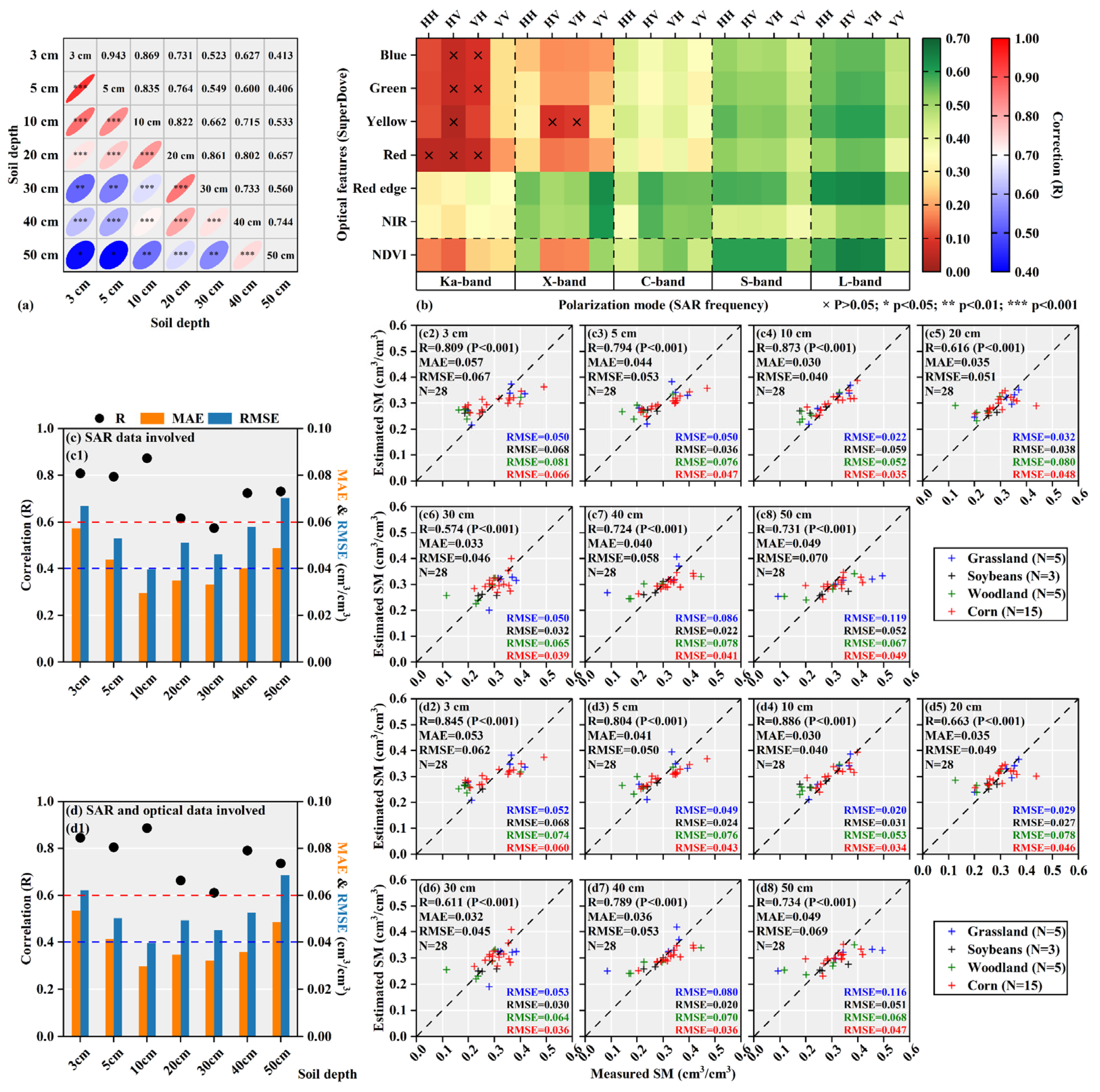
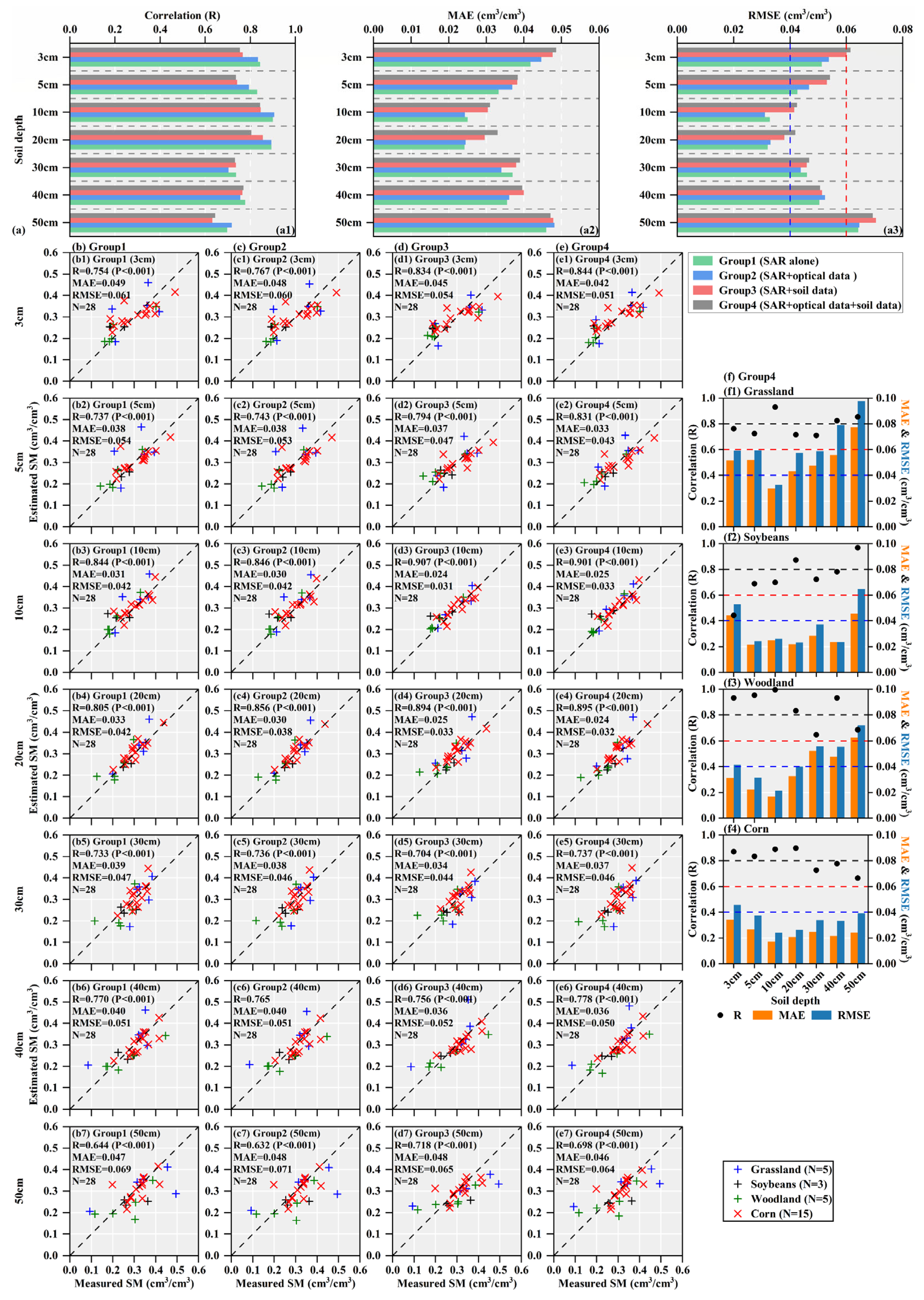
4.3.3. Evaluation of Multi-Layer and Profile Soil Moisture Estimation Accuracy Based on the Regression Model

As shown in Figure 7 and

Table A4. Estimation accuracy of multi-layer and profile SM based on the regression model.

Estimation Model	Accuracy Indices	Soil Depth
		3 cm	5 cm	10 cm	20 cm	30 cm	40 cm	50 cm
Group1	R	0.754	0.737	0.844	0.805	0.733	0.770	0.644
	MAE	0.049	0.038	0.031	0.033	0.039	0.040	0.047
	RMSE	0.061	0.054	0.042	0.042	0.047	0.051	0.069
Group2	R	0.767	0.743	0.846	0.856	0.736	0.765	0.632
	MAE	0.048	0.038	0.030	0.030	0.038	0.040	0.048
	RMSE	0.060	0.053	0.042	0.038	0.046	0.051	0.071
Group3	R	0.834	0.794	0.907	0.894	0.704	0.756	0.718
	MAE	0.045	0.037	0.024	0.025	0.034	0.036	0.048
	RMSE	0.054	0.047	0.031	0.033	0.044	0.052	0.065
Group4	R	0.844	0.831	0.901	0.895	0.737	0.778	0.698
	MAE	0.042	0.033	0.025	0.024	0.037	0.036	0.046
	RMSE	0.051	0.043	0.033	0.032	0.046	0.050	0.064

Notes: Group1 represents GPR model using SAR data alone; Group2 represents GPR model using SAR and multispectral data; Group3 represents GPR model using SAR data and soil parameters; Group4 represents GPR model using SAR data, multispectral data, and soil parameters.

, a multi-input multi-output regression model (GPR model) was used to estimate the multi-layer and profile SM by coupling multi-source data, including the multi-frequency quad-pol SAR data (Ka-, X-, C-, S-, L-band), multispectral data (multi-band reflectance and optical vegetation index), and soil parameters (STT, SOM, and SR). Overall, when only the multi-frequency SAR data were used for modeling, the correlations (R) between the estimated and the measured values increased with soil depth but then declined below 30 cm. The estimation errors (MAE and RMSE) followed a trend of first decreasing and then increasing, with the lowest values at NSSM-10 cm and NSSM-20 cm, where the RMSE was approximately 0.040 cm³/cm³. Adding the multispectral data on top of the multi-frequency SAR data resulted in only a slight improvement in the SM estimation accuracy, whereas the inclusion of soil parameters led to a more significant improvement, though the differences across soil depths remained largely unchanged with the RMSE around 0.030 cm³/cm³. Similarly, there were notable differences in the estimation accuracy of the multi-layer and profile SM across different vegetation types. The estimation error followed a pattern of first decreasing and then increasing with soil depth, but the sensitive depth range varied among the vegetation types. For grassland, the correlation between the estimated and the measured values fluctuated around 0.800. NSSM-10 cm exhibited the highest estimation accuracy with an RMSE equal to 0.033 cm³/cm³, while SSM-3 cm, SSM-5 cm, NSSM-20 cm, and NSSM-30cm had comparable accuracy, with the RMSE below 0.060 cm³/cm³. However, the RZSM estimation errors exceed 0.080 cm³/cm³. For soybean, the SM penetration-sensitive depth ranged from 5 cm to 40 cm, with an RMSE between 0.023 cm³/cm³ and 0.037 cm³/cm³. For woodland, SM estimation accuracy at depths of 30 cm to 50 cm had an RMSE of about 0.060 cm³/cm³, which was significantly lower than that at depths of 0–20 cm where the RMSE was below 0.040 cm³/cm³. For corn, except for SSM-3 cm, the RMSE for all other depths were below 0.040 cm³/cm³, with the optimal depth range between 10 cm and 20 cm, where the RMSE was around 0.025 cm³/cm³.

In this study, the soil parameters used for SM regression modeling were obtained through field sampling, which ensured high sampling accuracy. In practical applications, existing high-resolution soil parameter products can be used, such as the ChinaSoilGrid—a national soil information dataset with a 90-m spatial resolution that includes various parameters like STTs and SOM [84,85]. Previous studies have shown that the accuracy of such soil products is generally acceptable and can support the development of SM estimation models [10,17]. Nonetheless, this study aims to investigate the upper bound of multi-layer and profile SM estimation accuracy. Therefore, in situ measured soil parameters were used to minimize the potential negative impact of measurement errors on the SM modeling.

4.4. Comparison with Other Studies

This study integrates high spatial resolution multi-frequency SAR data (Ka-, X-, C-, S-, and L-band), multispectral data, and soil parameters to construct a model for estimating the multi-layer and profile SM. It is necessary to select appropriate SAR frequencies and polarization modes based on different vegetation types to fully realize the potential of the multi-frequency SAR data in monitoring vegetation growth status, which is consistent with the perspectives of recent studies [83]. Compared with the previous studies that rely solely on single-frequency SAR data (L-band or C-band), this study fully exploits the unique penetration capabilities of airborne multi-frequency SAR data. Based on multi-polarization constraints and penetration depth weighting, SM at different depths is estimated simultaneously [33,34,38]. However, this study does not address the optimization of the SM retrieval process, such as solving the semi-empirical parameters of the WCM using physics-informed neural networks [64]. As a comparison to scattering models, this study also explores the upper limits of estimation accuracy for multi-layer and profile SM using advanced MLR algorithms (GPR model) [74,86].

The Xinzhou-60 platform is equipped with a P-band SAR sensor; however, it was unfortunately not activated for imaging during the AMFSEX sampling campaign. As a result, it could not be compared with the AirMOSS campaign, which has conducted long-term airborne P-band SAR observations and synchronous surface SM measurements [54]. With the successful launch of the European Space Agency’s BIOMASS satellite, the estimation and modeling of multi-layer and profile SM using P-band SAR data hold great promise for future applications [87,88,89]. Classic field observation campaigns, such as the SMAPVEX series (e.g., SMAPVEX12 and SMAPVEX16), collected time-series biophysical parameters and surface SM across dozens of plots, along with simultaneous acquisition of airborne/satellite SAR data. These efforts are beneficial for evaluating the temporal robustness of SM estimation models across different phenological stages. However, due to the lack of time-series airborne SAR data and in situ SM measurements, time-series regression algorithms such as transformers, were not considered for SM modeling in this study [38]. Polarimetric decomposition (PD) techniques can effectively decouple (separate) the “vegetation–soil” signals in the SAR data across different frequencies. However, due to calibration inaccuracies in the polarization channels of the airborne SAR data used in this study, PD techniques were not considered for SM estimation modeling [21,59,61,77].

5. Deficiencies and Prospects

This study did not evaluate the estimation accuracy of the existing multi-layer and profile SM products, mainly for the following reasons: First, the AMFSEX sampling campaign involved densely distributed surface sampling points located near coastal areas. Due to the relatively coarse spatial resolution of products, such as ERA5-Land, GLDAS, and SMAP datasets, there are masked regions (i.e., no valid values) along coastal boundaries. As a result, only a few grid pixels could be matched with the sampling points, making the derived statistical metrics meaningless. Second, the representation depths across different products are inconsistent [10]. For example, ERA5-Land products have a spatial resolution of 0.1° (approximately 9–10 km) and provide SM at depths of 0–7 cm, 7–28 cm, and 28–100 cm. GLDAS (v2.2) products have a spatial resolution of 0.25° (approximately 25–30 km) with SM at 10 cm, 40 cm, and 100 cm. SMAP (Level 4) products offer a spatial resolution of 9 km, with SM available for depths of 0–5 cm and 0–100 cm.

Due to airspace regulations, the flight plans for the airborne SAR platform during the AMFSEX campaign were issued around 8 a.m. on the same day, making it difficult to acquire the satellite SAR data with matching observation phases, such as Sentinel-1 (C-band), Gaofen-3 (C-band), and ALOS-2 (L-band). In addition, the flight altitude was relatively low. To ensure high spatial resolution imaging, the radar incidence angles were relatively large (>40°). Due to time constraints, vegetation water content measurements were omitted during the AMFSEX sampling campaign. The micro-topography of the sampling plots was relatively flat, with no distinct ridges or furrows, resulting in a smoother surface roughness. Therefore, this study ignored the adverse impact of SR on SM estimation using scattering models. Whether the proposed method in this study for estimating the multi-layer and profile SM is applicable to the multi-frequency satellite SAR data remains to be further investigated.

The potential sources of error in the SM estimation models used in this study may include the following: (1) For different vegetation types, the assumed maximum penetration depth of the multi-frequency SAR data may be unrealistic [83,90,91]. (2) The “theoretical” penetration depth calculated by the dielectric mixing model may contain certain inaccuracies [69,91]. (3) For sampling points with high vegetation cover, the vegetation scattering component may not be fully removed in the scattering model, resulting in residual vegetation signal interference in the bare soil component [92]. (4) The estimation models do not consider the scattering effects of multi-frequency SAR signals between stratified soil layers [91,93]. (5) The system parameters of the airborne multi-frequency SAR data, such as radiometric resolution, are not uniform [59,94,95].

It should be noted that both the WCM and the GPR models used in this study rely on measured surface data. Once surface conditions change—such as vegetation growth status, STTs, or SM levels—the deployment and application of SM models may face significant challenges. In other words, the spatiotemporal transferability of SM estimation models still requires further investigation [17,31]. The AIR-CAS plans to conduct extensive high-resolution airborne imaging across various regions of mainland China over the next decade. Accordingly, we will carry out field synchronous observation campaigns aligned with these flight missions to further validate the spatiotemporal robustness of the multi-layer and profile SM estimation models developed in this study based on the multi-frequency SAR data. In addition, microwave anechoic chamber simulations should be used to clarify the penetration depth of the multi-frequency SAR data under complex surface conditions, thereby providing better guidance for multi-layer and profile SM estimation studies [96,97]. In conclusion, the acquisition of time-series high-resolution airborne multi-frequency quad-pol SAR data, combined with ground sampling, is essential for advancing SM estimation studies under varying vegetation types and phenological stages.

6. Conclusions

This study focused on high-resolution airborne multi-frequency quad-pol SAR data, including Ka-, X-, C-, S-, and L-band, with multispectral data and soil parameter data as auxiliary inputs to preliminarily construct multi-layer and profile SM estimation models. The main conclusions are as follows:

(1)

The sensitivity of the SAR data to biophysical parameters depends on its frequency, polarization mode, vegetation type, and biomass level. Overall, cross-polarization backscattering coefficients are more sensitive to biophysical parameters than co-polarization coefficients. High-frequency SAR data are more sensitive to low-biomass vegetation, while low-frequency SAR data are more responsive to high-biomass vegetation. Therefore, it is necessary to select appropriate SAR frequencies and polarization modes based on different vegetation types to fully realize the potential of the multi-frequency SAR data in monitoring vegetation growth status.

(2)

Due to variations in soil texture distribution and water demand, even when vegetation development in different sampling plots reached similar levels under the same climatic conditions, the SSM at depth 0–5 cm still exhibited significant heterogeneity. Similarly, because of differences between the soil layers, substantial heterogeneity existed in the measured multi-layer and profile SM even within the same vegetation type, including grassland, farmland, and woodland. Therefore, empirical models exhibited insufficient accuracy for fine-scale multi-layer and profile SM estimation.

(3)

The WCM based on multi-polarization weighting effectively reduced the adverse impact of vegetation scattering on SSM estimation. Among them, estimation accuracy using the L-band quad-pol SAR data met the monitoring requirement of RMSE < 0.060 cm³/cm³. The estimation accuracy of SSM was mainly influenced by SAR frequency, the dynamic range of SM content, vegetation types, and vegetation cover conditions.

(4)

The WCM constrained by multi-polarization weighting and penetration depth weighting fully leveraged the unique soil penetration sensitivity of the multi-frequency SAR data, thereby enabling accurate estimation of the multi-layer and profile SM across different vegetation types. The multi-input multi-output regression model effectively captured the complex relationships between multi-source data, including multi-frequency SAR, multispectral data, and soil physical/geometric parameters, and the measured multi-layer and profile SM, resulting in improved estimation accuracy. Regardless of whether the scattering model or the regression model was used, the overall SM penetration-sensitive depth range based on high-resolution airborne multi-frequency quad-pol SAR data was approximately 10–30 cm, and varied across different vegetation types.

References

1. Seneviratne, S.I.; Corti, T.; Davin, E.L.; Hirschi, M.; Jaeger, E.B.; Lehner, I.; Orlowsky, B.; Teuling, A.J. Investigating soil moisture–climate interactions in a changing climate: A review. Earth Sci. Rev. 2010, 99, 125–161. [Google Scholar] [CrossRef]
2. SU, S.L.; Singh, D.N.; Baghini, M.S. A critical review of soil moisture measurement. Measurement 2014, 54, 92–105. [Google Scholar] [CrossRef]
3. Zuo, Z.; Qiao, L.; Zhang, R.; Chen, D.; Piao, S.; Xiao, D.; Zhang, K. Importance of soil moisture conservation in mitigating climate change. Sci. Bull. 2024, 69, 1332–1341. [Google Scholar] [CrossRef]
4. Dorigo, W.; Wagner, W.; Albergel, C.; Albrecht, F.; Balsamo, G.; Brocca, L.; Chung, D.; Ertl, M.; Forkel, M.; Gruber, A.; et al. ESA CCI Soil Moisture for improved Earth system understanding: State-of-the art and future directions. Remote Sens. Environ. 2017, 203, 185–215. [Google Scholar] [CrossRef]
5. Wei, J.; Dirmeyer, P.A. Dissecting soil moisture-precipitation coupling. Geophys. Res. Lett. 2012, 39, L19711. [Google Scholar] [CrossRef]
6. Koster, R.D.; Suarez, M.J.; Higgins, R.W.; Van den Dool, H.M. Observational evidence that soil moisture variations affect precipitation. Geophys. Res. Lett. 2003, 30, 1241. [Google Scholar] [CrossRef]
7. AghaKouchak, A.; Farahmand, A.; Melton, F.S.; Teixeira, J.; Anderson, M.C.; Wardlow, B.D.; Hain, C.R. Remote sensing of drought: Progress, challenges and opportunities. Rev. Geophys. 2015, 53, 452–480. [Google Scholar] [CrossRef]
8. Rodriguez-Iturbe, I.; D’odorico, P.; Porporato, A.; Ridolfi, L. On the spatial and temporal links between vegetation, climate, and soil moisture. Water Resour. Res. 1999, 35, 3709–3722. [Google Scholar] [CrossRef]
9. Li, W.; Migliavacca, M.; Forkel, M.; Denissen, J.M.; Reichstein, M.; Yang, H.; Duveiller, G.; Weber, U.; Orth, R. Widespread increasing vegetation sensitivity to soil moisture. Nat. Commun. 2022, 13, 3959. [Google Scholar] [CrossRef]
10. Qian, J.; Yang, J.; Sun, W.; Zhao, L.; Shi, L.; Shi, H.; Dang, C.; Dou, Q. Application potential and spatiotemporal uncertainty assessment of multi-layer soil moisture estimation in different climate zones using multi-source data. J. Hydrol. 2024, 645, 132229. [Google Scholar] [CrossRef]
11. Karthikeyan, L.; Mishra, A.K. Multi-layer high-resolution soil moisture estimation using machine learning over the United States. Remote Sens. Environ. 2021, 266, 112706. [Google Scholar] [CrossRef]
12. Wang, L.; Qu, J.J. Satellite remote sensing applications for surface soil moisture monitoring: A review. Front. Earth Sci. China 2009, 3, 237–247. [Google Scholar] [CrossRef]
13. Xue, S.; Wu, G. Causal inference of root zone soil moisture performance in drought. Agric. Water Manag. 2024, 305, 109123. [Google Scholar] [CrossRef]
14. Tian, J.; Zhang, Y.; Guo, J.; Zhang, X.; Ma, N.; Wei, H.; Tang, Z. Predicting root zone soil moisture using observations at 2121 sites across China. Sci. Total Environ. 2022, 847, 157425. [Google Scholar] [CrossRef]
15. Li, N.; Skaggs, T.H.; Ellegaard, P.; Bernal, A.; Scudiero, E. Relationships among soil moisture at various depths under diverse climate, land cover and soil texture. Sci. Total Environ. 2024, 947, 174583. [Google Scholar] [CrossRef]
16. Sun, P.; Liu, R.; Yao, R.; Shen, H.; Bian, Y. Responses of agricultural drought to meteorological drought under different climatic zones and vegetation types. J. Hydrol. 2023, 619, 129305. [Google Scholar] [CrossRef]
17. Qian, J.; Yang, J.; Sun, W.; Zhao, L.; Shi, L.; Shi, H.; Liao, L.; Dang, C.; Dou, Q. Evaluation and improvement of spatiotemporal estimation and transferability of multi-layer and profile soil moisture in the Qinghai Lake and Heihe River basins using multi-strategy constraints. Geoderma 2025, 455, 117222. [Google Scholar] [CrossRef]
18. Kim, S.-B.; Liao, T.-H. Robust retrieval of soil moisture at field scale across wide-ranging SAR incidence angles for soybean, wheat, forage, oat and grass. Remote Sens. Environ. 2021, 266, 112712. [Google Scholar] [CrossRef]
19. Yadav, V.P.; Prasad, R.; Bala, R.; Vishwakarma, A.K. An improved inversion algorithm for spatio-temporal retrieval of soil moisture through modified water cloud model using C-band Sentinel-1A SAR data. Comput. Electron. Agric. 2020, 173, 105447. [Google Scholar] [CrossRef]
20. Balenzano, A.; Mattia, F.; Satalino, G.; Davidson, M.W. Dense temporal series of C-and L-band SAR data for soil moisture retrieval over agricultural crops. IEEE J. Sel. Top. Appl. Earth Obs. Remote Sens. 2010, 4, 439–450. [Google Scholar] [CrossRef]
21. Shi, H.; Zhao, L.; Yang, J.; Lopez-Sanchez, J.M.; Zhao, J.; Sun, W.; Shi, L.; Li, P. Soil moisture retrieval over agricultural fields from L-band multi-incidence and multitemporal PolSAR observations using polarimetric decomposition techniques. Remote Sens. Environ. 2021, 261, 112485. [Google Scholar] [CrossRef]
22. Dorigo, W.; Himmelbauer, I.; Aberer, D.; Schremmer, L.; Petrakovic, I.; Zappa, L.; Preimesberger, W.; Xaver, A.; Annor, F.; Ardö, J. The International Soil Moisture Network: Serving Earth system science for over a decade. Hydrol. Earth Syst. Sci. 2021, 25, 5749–5804. [Google Scholar] [CrossRef]
23. Liu, Y.; Qian, J.; Yue, H. Comprehensive evaluation of Sentinel-2 red edge and shortwave-infrared bands to estimate soil moisture. IEEE J. Sel. Top. Appl. Earth Obs. Remote Sens. 2021, 14, 7448–7465. [Google Scholar] [CrossRef]
24. Liu, Y.; Qian, J.; Yue, H. Combined Sentinel-1A with Sentinel-2A to estimate soil moisture in farmland. IEEE J. Sel. Top. Appl. Earth Obs. Remote Sens. 2020, 14, 1292–1310. [Google Scholar] [CrossRef]
25. Kerr, Y.H.; Waldteufel, P.; Richaume, P.; Wigneron, J.P.; Ferrazzoli, P.; Mahmoodi, A.; Al Bitar, A.; Cabot, F.; Gruhier, C.; Juglea, S.E. The SMOS soil moisture retrieval algorithm. IEEE Trans. Geosci. Remote Sens. 2012, 50, 1384–1403. [Google Scholar] [CrossRef]
26. Entekhabi, D.; Njoku, E.G.; O’neill, P.E.; Kellogg, K.H.; Crow, W.T.; Edelstein, W.N.; Entin, J.K.; Goodman, S.D.; Jackson, T.J.; Johnson, J. The soil moisture active passive (SMAP) mission. Proc. IEEE 2010, 98, 704–716. [Google Scholar] [CrossRef]
27. Dang, C.; Shao, Z.; Huang, X.; Qian, J.; Cheng, G.; Ding, Q.; Fan, Y. Assessment of the importance of increasing temperature and decreasing soil moisture on global ecosystem productivity using solar-induced chlorophyll fluorescence. Glob. Change Biol. 2021, 28, 2066–2080. [Google Scholar] [CrossRef]
28. Chan, S.K.; Bindlish, R.; O’Neill, P.E.; Njoku, E.; Jackson, T.; Colliander, A.; Chen, F.; Burgin, M.; Dunbar, S.; Piepmeier, J. Assessment of the SMAP passive soil moisture product. IEEE Trans. Geosci. Remote Sens. 2016, 54, 4994–5007. [Google Scholar] [CrossRef]
29. Peng, J.; Loew, A.; Merlin, O.; Verhoest, N.E. A review of spatial downscaling of satellite remotely sensed soil moisture. Rev. Geophys. 2017, 55, 341–366. [Google Scholar] [CrossRef]
30. Karthikeyan, L.; Pan, M.; Wanders, N.; Kumar, D.N.; Wood, E.F. Four decades of microwave satellite soil moisture observations: Part 1. A review of retrieval algorithms. Adv. Water Resour. 2017, 109, 106–120. [Google Scholar] [CrossRef]
31. Zhu, L.; Dai, J.; Liu, Y.; Yuan, S.; Qin, T.; Walker, J.P. A cross-resolution transfer learning approach for soil moisture retrieval from Sentinel-1 using limited training samples. Remote Sens. Environ. 2024, 301, 113944. [Google Scholar] [CrossRef]
32. Zhao, T.; Hu, L.; Shi, J.; Lü, H.; Li, S.; Fan, D.; Wang, P.; Geng, D.; Kang, C.S.; Zhang, Z. Soil moisture retrievals using L-band radiometry from variable angular ground-based and airborne observations. Remote Sens. Environ. 2020, 248, 111958. [Google Scholar] [CrossRef]
33. Colliander, A.; Cosh, M.H.; Misra, S.; Jackson, T.J.; Crow, W.T.; Powers, J.; McNairn, H.; Bullock, P.; Berg, A.; Magagi, R. Comparison of high-resolution airborne soil moisture retrievals to SMAP soil moisture during the SMAP validation experiment 2016 (SMAPVEX16). Remote Sens. Environ. 2019, 227, 137–150. [Google Scholar] [CrossRef]
34. Bhogapurapu, N.; Dey, S.; Mandal, D.; Bhattacharya, A.; Karthikeyan, L.; McNairn, H.; Rao, Y.S. Soil moisture retrieval over croplands using dual-pol L-band GRD SAR data. Remote Sens. Environ. 2022, 271, 112900. [Google Scholar] [CrossRef]
35. Singh, S.K.; Prasad, R.; Srivastava, P.K.; Yadav, S.A.; Yadav, V.P.; Sharma, J. Incorporation of first-order backscattered power in Water Cloud Model for improving the Leaf Area Index and Soil Moisture retrieval using dual-polarized Sentinel-1 SAR data. Remote Sens. Environ. 2023, 296, 113756. [Google Scholar] [CrossRef]
36. Park, S.-E.; Jung, Y.T.; Cho, J.-H.; Moon, H.; Han, S.-h. Theoretical evaluation of water cloud model vegetation parameters. Remote Sens. 2019, 11, 894. [Google Scholar] [CrossRef]
37. Zhu, L.; Si, R.; Shen, X.; Walker, J.P. An advanced change detection method for time-series soil moisture retrieval from Sentinel-1. Remote Sens. Environ. 2022, 279, 113137. [Google Scholar] [CrossRef]
38. Zhu, L.; Dai, J.; Jin, J.; Yuan, S.; Xiong, Z.; Walker, J.P. Are the current expectations for SAR remote sensing of soil moisture using machine learning over-optimistic? IEEE Trans. Geosci. Remote Sens. 2025, 63, 1–15. [Google Scholar]
39. Zheng, X.; Feng, Z.; Li, L.; Li, B.; Jiang, T.; Li, X.; Li, X.; Chen, S. Simultaneously estimating surface soil moisture and roughness of bare soils by combining optical and radar data. Int. J. Appl. Earth Obs. Geoinf. 2021, 100, 102345. [Google Scholar] [CrossRef]
40. Reichle, R.H. Data assimilation methods in the Earth sciences. Adv. Water Resour. 2008, 31, 1411–1418. [Google Scholar] [CrossRef]
41. Muñoz-Sabater, J.; Dutra, E.; Agustí-Panareda, A.; Albergel, C.; Arduini, G.; Balsamo, G.; Boussetta, S.; Choulga, M.; Harrigan, S.; Hersbach, H. ERA5-Land: A state-of-the-art global reanalysis dataset for land applications. Earth Syst. Sci. Data 2021, 13, 4349–4383. [Google Scholar] [CrossRef]
42. Rodell, M.; Houser, P.; Jambor, U.; Gottschalck, J.; Mitchell, K.; Meng, C.-J.; Arsenault, K.; Cosgrove, B.; Radakovich, J.; Bosilovich, M. The global land data assimilation system. Bull. Am. Meteorol. Soc. 2004, 85, 381–394. [Google Scholar] [CrossRef]
43. Gelaro, R.; McCarty, W.; Suárez, M.J.; Todling, R.; Molod, A.; Takacs, L.; Randles, C.A.; Darmenov, A.; Bosilovich, M.G.; Reichle, R. The modern-era retrospective analysis for research and applications, version 2 (MERRA-2). J. Clim. 2017, 30, 5419–5454. [Google Scholar] [CrossRef]
44. Shi, C.; Xie, Z.; Qian, H.; Liang, M.; Yang, X. China land soil moisture EnKF data assimilation based on satellite remote sensing data. Sci. China Earth Sci. 2011, 54, 1430–1440. [Google Scholar] [CrossRef]
45. Miralles, D.G.; Holmes, T.; De Jeu, R.; Gash, J.; Meesters, A.; Dolman, A. Global land-surface evaporation estimated from satellite-based observations. Hydrol. Earth Syst. Sci. 2011, 15, 453–469. [Google Scholar] [CrossRef]
46. Zhao, T.; Shi, J.; Lv, L.; Xu, H.; Chen, D.; Cui, Q.; Jackson, T.J.; Yan, G.; Jia, L.; Chen, L.; et al. Soil moisture experiment in the Luan River supporting new satellite mission opportunities. Remote Sens. Environ. 2020, 240, 111680. [Google Scholar] [CrossRef]
47. Ahmad, S.; Kalra, A.; Stephen, H. Estimating soil moisture using remote sensing data: A machine learning approach. Adv. Water Resour. 2010, 33, 69–80. [Google Scholar] [CrossRef]
48. Singh, A.; Gaurav, K. PIML-SM: Physics-informed machine learning to estimate surface soil moisture from multi-sensor satellite images by leveraging swarm intelligence. IEEE Trans. Geosci. Remote Sens. 2024, 62, 1–13. [Google Scholar] [CrossRef]
49. Zhang, M.; Zhang, D.; Jin, Y.; Wan, X.; Ge, Y. Evolution of soil moisture mapping from statistical models to integrated mechanistic and geoscience-aware approaches. Inf. Geogr. 2025, 1, 100005. [Google Scholar] [CrossRef]
50. McNairn, H.; Jackson, T.J.; Wiseman, G.; Belair, S.; Berg, A.; Bullock, P.; Colliander, A.; Cosh, M.H.; Kim, S.-B.; Magagi, R. The soil moisture active passive validation experiment 2012 (SMAPVEX12): Prelaunch calibration and validation of the SMAP soil moisture algorithms. IEEE Trans. Geosci. Remote Sens. 2014, 53, 2784–2801. [Google Scholar] [CrossRef]
51. Mengen, D.; Montzka, C.; Jagdhuber, T.; Fluhrer, A.; Brogi, C.; Baum, S.; Schüttemeyer, D.; Bayat, B.; Bogena, H.; Coccia, A. The SARSense campaign: Air-and space-borne C-and L-band SAR for the analysis of soil and plant parameters in agriculture. Remote Sens. 2021, 13, 825. [Google Scholar] [CrossRef]
52. Zhao, T.; Shi, J.; Entekhabi, D.; Jackson, T.J.; Hu, L.; Peng, Z.; Yao, P.; Li, S.; Kang, C.S. Retrievals of soil moisture and vegetation optical depth using a multi-channel collaborative algorithm. Remote Sens. Environ. 2021, 257, 112321. [Google Scholar] [CrossRef]
53. Jackson, T.J.; Le Vine, D.M.; Hsu, A.Y.; Oldak, A.; Starks, P.J.; Swift, C.T.; Isham, J.D.; Haken, M. Soil moisture mapping at regional scales using microwave radiometry: The Southern Great Plains Hydrology Experiment. IEEE Trans. Geosci. Remote Sens. 1999, 37, 2136–2151. [Google Scholar] [CrossRef]
54. Tabatabaeenejad, A.; Burgin, M.; Duan, X.; Moghaddam, M. P-Band Radar Retrieval of Subsurface Soil Moisture Profile as a Second-Order Polynomial: First AirMOSS Results. IEEE Trans. Geosci. Remote Sens. 2014, 53, 645–658. [Google Scholar] [CrossRef]
55. Hajnsek, I.; Bianchi, R.; Davidson, M.; D’Urso, G.; Gomez-Sanchez, J.; Hausold, A.; Horn, R.; Howse, J.; Loew, A.; Lopez-Sanchez, J. AgriSAR 2006—Airborne SAR and optics campaigns for an improved monitoring of agricultural processes and practices. In Proceedings of the Geophysical Research Abstracts, Vienna, Austria, 15–20 April 2007; p. 04085. [Google Scholar]
56. Panciera, R.; Walker, J.P.; Jackson, T.J.; Gray, D.A.; Tanase, M.A.; Ryu, D.; Monerris, A.; Yardley, H.; Rüdiger, C.; Wu, X. The soil moisture active passive experiments (SMAPEx): Toward soil moisture retrieval from the SMAP mission. IEEE Trans. Geosci. Remote Sens. 2013, 52, 490–507. [Google Scholar] [CrossRef]
57. Peischl, S.; Walker, J.P.; Rüdiger, C.; Ye, N.; Kerr, Y.H.; Kim, E.; Bandara, R.; Allahmoradi, M. The AACES field experiments: SMOS calibration and validation across the Murrumbidgee River catchment. Hydrol. Earth Syst. Sci. 2012, 16, 1697–1708. [Google Scholar] [CrossRef]
58. Kang, J.; Jin, R.; Li, X.; Ma, M. HIWATER: WATERNET Observation Dataset in the Upper Reaches of the Heihe River Basin in 2014; Heihe Plan Science Data Center: Beijing, China, 2015. [Google Scholar]
59. Wu, Y.; Ding, C.; Wang, B.; Jiao, Z.; Zhou, L.; Wang, R. Multi-dimensional Imaging with MD-JoSAR Mission in China: Challenges and Opportunities. In Proceedings of the EUSAR 2024; 15th European Conference on Synthetic Aperture Radar, Munich, Germany, 23–26 April 2024; pp. 989–994. [Google Scholar]
60. Wang, Z.; Zhao, T.; Shi, J.; Wang, H.; Ji, D.; Yao, P.; Zheng, J.; Zhao, X.; Xu, X. 1-km soil moisture retrieval using multi-temporal dual-channel SAR data from Sentinel-1 A/B satellites in a semi-arid watershed. Remote Sens. Environ. 2023, 284, 113334. [Google Scholar] [CrossRef]
61. Dou, Q.; Xie, Q.; Peng, X.; Lai, K.; Wang, J.; Lopez-Sanchez, J.M.; Shang, J.; Shi, H.; Fu, H.; Zhu, J. Soil moisture retrieval over crop fields based on two-component polarimetric decomposition: A comparison of generalized volume scattering models. J. Hydrol. 2022, 615, 128696. [Google Scholar] [CrossRef]
62. Li, J.; Wang, S. Using SAR-Derived Vegetation Descriptors in a Water Cloud Model to Improve Soil Moisture Retrieval. Remote Sens. 2018, 10, 1370. [Google Scholar] [CrossRef]
63. Attema, E.; Ulaby, F.T. Vegetation modeled as a water cloud. Radio Sci. 1978, 13, 357–364. [Google Scholar] [CrossRef]
64. Li, Z.; Yuan, Q.; Yang, Q.; Li, J.; Zhao, T. Differentiable modeling for soil moisture retrieval by unifying deep neural networks and water cloud model. Remote Sens. Environ. 2024, 311, 114281. [Google Scholar] [CrossRef]
65. Bao, Y.; Lin, L.; Wu, S.; Kwal Deng, K.A.; Petropoulos, G.P. Surface soil moisture retrievals over partially vegetated areas from the synergy of Sentinel-1 and Landsat 8 data using a modified water-cloud model. Int. J. Appl. Earth Obs. Geoinf. 2018, 72, 76–85. [Google Scholar] [CrossRef]
66. Baghdadi, N.; El Hajj, M.; Zribi, M.; Bousbih, S. Calibration of the Water Cloud Model at C-Band for Winter Crop Fields and Grasslands. Remote Sens. 2017, 9, 969. [Google Scholar] [CrossRef]
67. Wang, Z.; Zhao, T.; Qiu, J.; Zhao, X.; Li, R.; Wang, S. Microwave-based vegetation descriptors in the parameterization of water cloud model at L-band for soil moisture retrieval over croplands. GISci. Remote Sens. 2021, 58, 48–67. [Google Scholar] [CrossRef]
68. Hosseini, M.; McNairn, H. Using multi-polarization C-and L-band synthetic aperture radar to estimate biomass and soil moisture of wheat fields. Int. J. Appl. Earth Obs. Geoinf. 2017, 58, 50–64. [Google Scholar] [CrossRef]
69. Singh, A.; Niranjannaik, M.; Kumar, S.; Gaurav, K. Comparison of different dielectric models to estimate penetration depth of l-and s-band sar signals into the ground surface. Geographies 2022, 2, 734–742. [Google Scholar] [CrossRef]
70. Dobson, M.C.; Ulaby, F.T.; Hallikainen, M.T.; El-Rayes, M.A. Microwave dielectric behavior of wet soil-Part II: Dielectric mixing models. IEEE Trans. Geosci. Remote Sens. 1985, 23, 35–46. [Google Scholar] [CrossRef]
71. Hallikainen, M.T.; Ulaby, F.T.; Dobson, M.C.; El-Rayes, M.A.; Wu, L.-K. Microwave dielectric behavior of wet soil-part 1: Empirical models and experimental observations. IEEE Trans. Geosci. Remote Sens. 1985, GE-23, 25–34. [Google Scholar] [CrossRef]
72. Williams, C.; Rasmussen, C. Gaussian processes for regression. Adv. Neural Inf. Process. Syst. 1995, 8, 514–520. [Google Scholar]
73. Schulz, E.; Speekenbrink, M.; Krause, A. A tutorial on Gaussian process regression: Modelling, exploring, and exploiting functions. J. Math. Psychol. 2018, 85, 1–16. [Google Scholar] [CrossRef]
74. Xue, Z.; Zhang, Y.; Zhang, L.; Li, H. Ensemble Learning Embedded With Gaussian Process Regression for Soil Moisture Estimation: A Case Study of the Continental US. IEEE Trans. Geosci. Remote Sens. 2022, 60, 1–17. [Google Scholar] [CrossRef]
75. Qian, J.; Jie, Y.; Weidong, S.; Lingli, Z.; Lei, S.; Chaoya, D. Evaluation and improvement of temporal robustness and transfer performance of surface soil moisture estimated by machine learning regression algorithms. Comput. Electron. Agric. 2024, 217, 108518. [Google Scholar]
76. Wu, J.; Chen, X.-Y.; Zhang, H.; Xiong, L.-D.; Lei, H.; Deng, S.-H. Hyperparameter optimization for machine learning models based on Bayesian optimization. J. Electron. Sci. Technol. 2019, 17, 26–40. [Google Scholar]
77. Wang, H.; Magagi, R.; Goïta, K. Potential of a two-component polarimetric decomposition at C-band for soil moisture retrieval over agricultural fields. Remote Sens. Environ. 2018, 217, 38–51. [Google Scholar] [CrossRef]
78. Wang, J.; Wu, F.; Shang, J.; Zhou, Q.; Ahmad, I.; Zhou, G. Saline soil moisture mapping using Sentinel-1A synthetic aperture radar data and machine learning algorithms in humid region of China’s east coast. Catena 2022, 213, 106189. [Google Scholar] [CrossRef]
79. Peraza, J.; Rossini, P.R.; Patrignani, A. Mapping mesoscale soil moisture using a model-data fusion approach. J. Hydrol. 2025, 654, 132768. [Google Scholar] [CrossRef]
80. Wimalathunge, N.; Bishop, T. A space-time observation system for soil moisture in agricultural landscapes. Geoderma 2019, 344, 1–13. [Google Scholar] [CrossRef]
81. Liu, D.; Mishra, A.K.; Yu, Z. Evaluating uncertainties in multi-layer soil moisture estimation with support vector machines and ensemble Kalman filtering. J. Hydrol. 2016, 538, 243–255. [Google Scholar] [CrossRef]
82. Singh, A.; Meena, G.K.; Kumar, S.; Gaurav, K. Analysis of the effect of incidence angle and moisture content on the penetration depth of L-and S-band SAR signals into the ground surface. ISPRS Ann. Photogramm. Remote Sens. Spat. Inf. Sci. 2018, 4, 197–202. [Google Scholar] [CrossRef]
83. Roßberg, T.; Schmitt, M. Comparing the relationship between NDVI and SAR backscatter across different frequency bands in agricultural areas. Remote Sens. Environ. 2025, 319, 114612. [Google Scholar] [CrossRef]
84. Liu, F.; Zhang, G.-L.; Song, X.; Li, D.; Zhao, Y.; Yang, J.; Wu, H.; Yang, F. High-resolution and three-dimensional mapping of soil texture of China. Geoderma 2020, 361, 114061. [Google Scholar] [CrossRef]
85. Liu, F.; Wu, H.; Zhao, Y.; Li, D.; Yang, J.-L.; Song, X.; Shi, Z.; Zhu, A.X.; Zhang, G.-L. Mapping high resolution National Soil Information Grids of China. Sci. Bull. 2022, 67, 328–340. [Google Scholar] [CrossRef] [PubMed]
86. Rasmussen, C.E. Gaussian processes in machine learning. In Proceedings of the Summer School on Machine Learning, Canberra, Australia, 2–14 February 2003; pp. 63–71. [Google Scholar]
87. Fluhrer, A.; Jagdhuber, T.; Montzka, C.; Schumacher, M.; Alemohammad, H.; Tabatabaeenejad, A.; Kunstmann, H.; Entekhabi, D. Soil moisture profile estimation by combining P-band SAR polarimetry with hydrological and multi-layer scattering models. Remote Sens. Environ. 2024, 305, 114067. [Google Scholar] [CrossRef]
88. Scipal, K. The Biomass mission—ESA’S P-band polarimetric, interferomtric SAR mission. In Proceedings of the 2017 IEEE International Geoscience and Remote Sensing Symposium (IGARSS), Fort Worth, TX, USA, 23–28 July 2017; pp. 3836–3837. [Google Scholar]
89. Fluhrer, A.; Jagdhuber, T.; Tabatabaeenejad, A.; Alemohammad, H.; Montzka, C.; Friedl, P.; Forootan, E.; Kunstmann, H. Remote sensing of complex permittivity and penetration depth of soils using P-band SAR polarimetry. Remote Sens. 2022, 14, 2755. [Google Scholar] [CrossRef]
90. El Hajj, M.; Baghdadi, N.; Bazzi, H.; Zribi, M. Penetration analysis of SAR signals in the C and L bands for wheat, maize, and grasslands. Remote Sens. 2018, 11, 31. [Google Scholar] [CrossRef]
91. Zhu, J.; Liu, G.; Zhao, R.; Ding, X.; Fu, H. ML based approach for inverting penetration depth of SAR signals over large desert areas. Remote Sens. Environ. 2023, 295, 113643. [Google Scholar] [CrossRef]
92. Capodici, F.; Maltese, A.; Ciraolo, G.; D’Urso, G.; La Loggia, G. Power sensitivity analysis of multi-frequency, multi-polarized, multi-temporal SAR data for soil-vegetation system variables characterization. Remote Sens. 2017, 9, 677. [Google Scholar] [CrossRef]
93. Abdikan, S.; Sekertekin, A.; Madenoglu, S.; Ozcan, H.; Peker, M.; Pinar, M.O.; Koc, A.; Akgul, S.; Secmen, H.; Kececi, M. Surface soil moisture estimation from multi-frequency SAR images using ANN and experimental data on a semi-arid environment region in Konya, Turkey. Soil Tillage Res. 2023, 228, 105646. [Google Scholar] [CrossRef]
94. Yao, Z.; Dong, Q.; Song, C.; Jiao, Z.; Wang, B.; Xiang, M. MD-JoSAR Imaging System and Application Based on Multidimensional Joint Spatial Observations. In Proceedings of the 2024 Photonics & Electromagnetics Research Symposium (PIERS), Chengdu, China, 21–25 April 2024; pp. 1–8. [Google Scholar]
95. Li, L.; Zhang, F.; Shao, Y.; Wei, Q.; Huang, Q.; Jiao, Y. Airborne SAR radiometric calibration based on improved sliding window integral method. Sensors 2022, 22, 320. [Google Scholar] [CrossRef]
96. Ruan, L.; Liu, Z.; Shao, Y.; Xiao, X.; Zhang, T.; Bian, X.; Zhang, N.; Wu, X. Radar Backscattering Characterization of Soil Surface: Comparisons between Backscattering Models and Indoor Microwave Measurements. In Proceedings of the 2023 International Applied Computational Electromagnetics Society Symposium (ACES-China), Hangzhou, China, 15–18 August 2023; pp. 1–3. [Google Scholar]
97. Liu, X.; Shao, Y.; Li, K.; Liu, Z.; Liu, L.; Xiao, X. Backscattering Statistics of Indoor Full-Polarization Scatterometric and Synthetic Aperture Radar Measurements of a Rice Field. Remote Sens. 2023, 15, 965. [Google Scholar] [CrossRef]
Figure 1. (a) Geographic location of the study area. (b) Land use classification map. (c,d) SuperDove images of the sampling area (18 July 2023, 8 August 2023; the green dots). (e) Airborne SAR imaging coverage. (f) Ground corner reflector deployment locations (the green cross). (g) Field photos of typical vegetation in the study area.
Water 17 02096 g001
Figure 2. Multi-frequency SAR images of typical vegetation in the AMFSEX experiment: (a) grassland; (b) soybeans; (c) woodland; (d) corn. From left to right are the Ka- (0.3 m), X- (0.5 m), C- (0.5 m), S- (1.0 m), and L-band (1.0 m) SAR images and the corresponding SuperDove images with standard false color synthesis. The red and yellow cross shapes represent the sampling points. The black area in (c) is the SAR imaging shadow caused by high radar incident angles.
Water 17 02096 g002
Figure 3. Measured SSM (0–5 cm), STT, and vegetation growth conditions in the sampling plots. (a) Measured SSM box patterns of the different sampling plots. (b) The proportion of STT and SOM of the different sample plots. (c) NDVI derived from the SuperDove images and the measured LAI of different sampling plots. (d) The relationship between the NDVI derived from the SuperDove images and the measured LAI of different sampling plots.
Water 17 02096 g003
Figure 4. Simulation results of multi-frequency SAR signal soil penetration capability based on the Dobson model and the Hallikainen model: (a) Dobson model for L-band; (b) Hallikainen model for L-band; (c) Dobson model for C-band; (d) Hallikainen model for C-band. (a1a4) represent the radar incidence angle at 20°, 30°, 40°, and 50°, respectively. The same is true for the other subgraphs.
Water 17 02096 g004
Figure 5. Estimation accuracy of SSM (0–5 cm) for different vegetation types based on the scattering model and the regression model. (a) Estimation accuracy based on the WCM: (a1) involving the SAR data alone, (a2) involving the SAR and multispectral data. (b) Estimation results based on the WCM involving the SAR data alone. (c) Estimation results based on the WCM involving SAR and multispectral data. (d) Estimation results based on the GPR model involving SAR and multispectral data. (b1b5) represent the Ka-, X-, C-, S-, and L-band, respectively. The same is true for the other subgraphs.
Water 17 02096 g005
Figure 6. Estimation accuracy of multi-layer and profile SM based on the scattering model. (a) Correlation among measured SM at different depths. (b) Correlation between radar backscattering coefficients at different frequencies and the SuperDove multispectral reflectance and the NDVI for the sampling plots. (c) Estimation accuracy of the WCM constrained by multi-polarization weighting and penetration depth weighting (considering only the SAR data). Note: (c2c8) represent the SM estimation results at depths of 3 cm, 5 cm, 10 cm, 20 cm, 30 cm, 40 cm, and 50 cm, respectively; (d) is the same as (c), but considering both the SAR and multispectral data; (d2d8) correspond to (c2c8), respectively.
Water 17 02096 g006
Figure 7. Estimation accuracy of multi-layer and profile SM based on the regression model. (a) Estimation accuracy under different feature sets: (a1) correlation (R); (a2) MAE; (a3) RMSE. (be) Represent estimation results under different feature sets: (b) using the SAR data alone; (c) using SAR and multispectral data; (d) using the SAR data and soil parameters; (e) using the SAR data, multispectral data, and soil parameters. (b1b7) represent estimation results at depths of 3 cm, 5 cm, 10 cm, 20 cm, 30 cm, 40 cm, and 50 cm, respectively; the same applies to the other subplots. (f) Estimation accuracy of multi-layer and profile SM under different vegetation cover types when multi-source data are used: (f1) grassland; (f2) soybeans; (f3) woodland; (f4) corn.
Water 17 02096 g007