
Leveraging Advanced Data-Driven Approaches to Forecast Daily Floods Based on Rainfall for Proactive Prevention Strategies in Saudi Arabia


Abstract
1. Introduction
Background
2. Materials and Methods
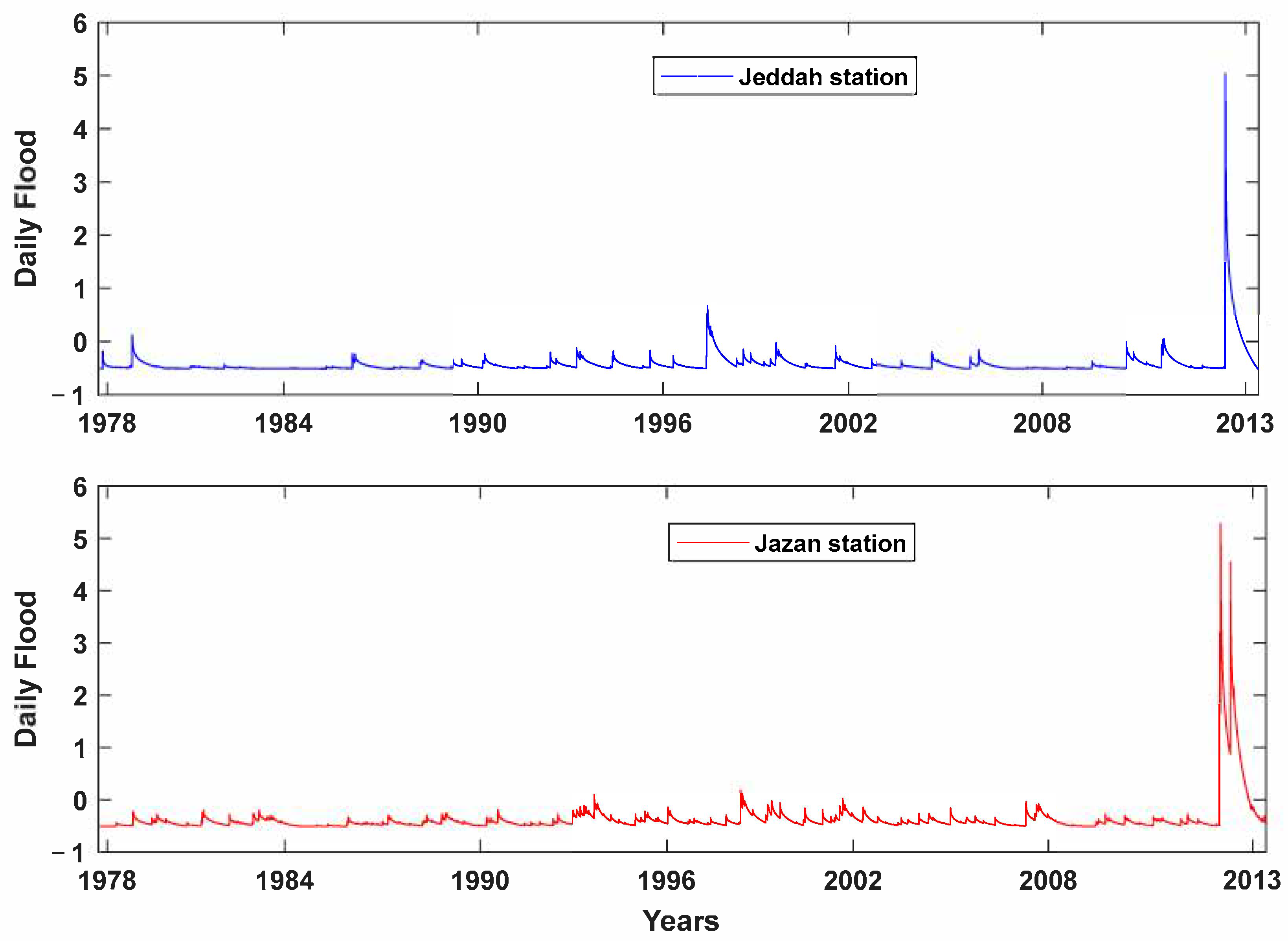
2.1. Study Area and Data Description
2.2. Variational Mode Decomposition (VMD)
2.3. Gaussian Process Regression (GPR)
2.4. Long Short-Term Memory (LSTM)
2.5. Boosted Regression Tree (BRT)
2.6. Cascaded Forward Neural Network (CFNN)
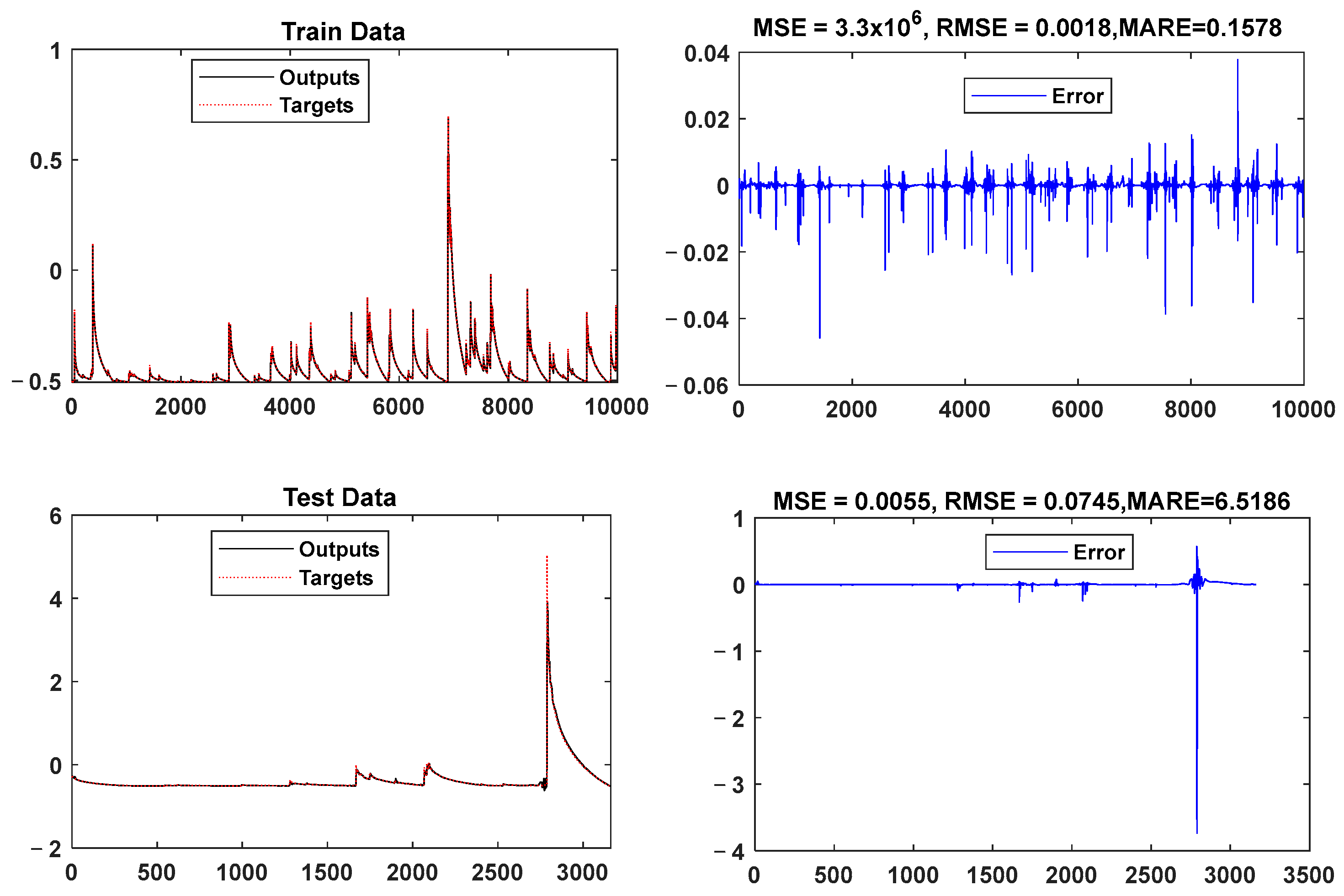
2.7. Model Performance Evaluation Criteria
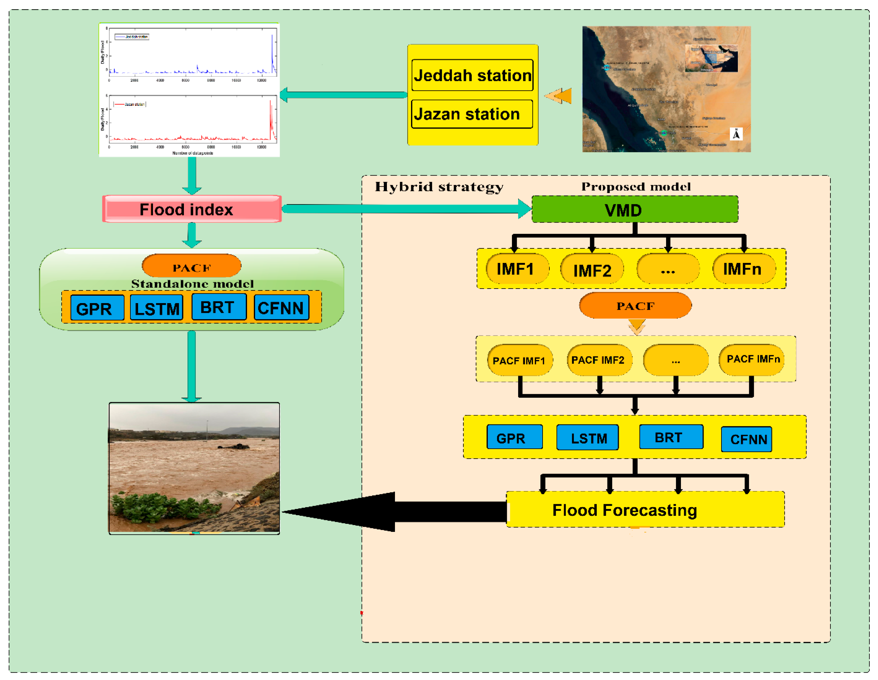
2.8. Model Development
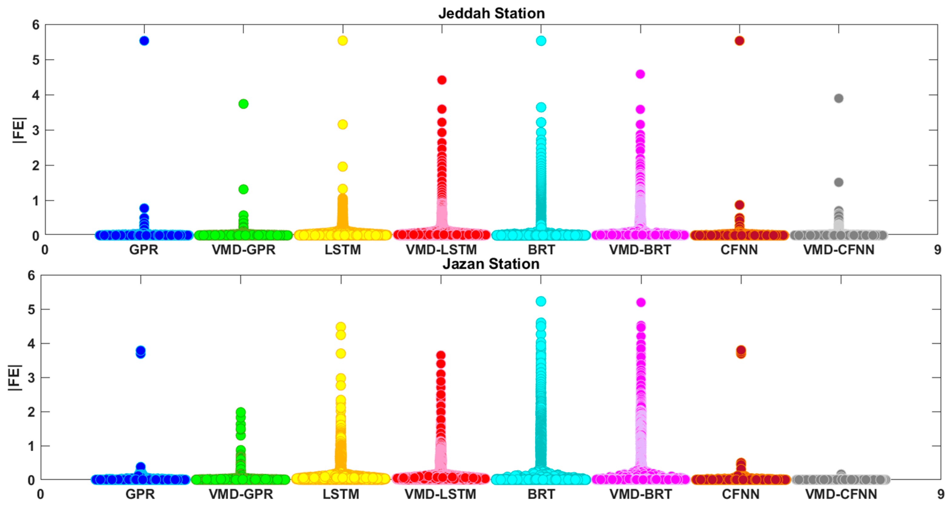
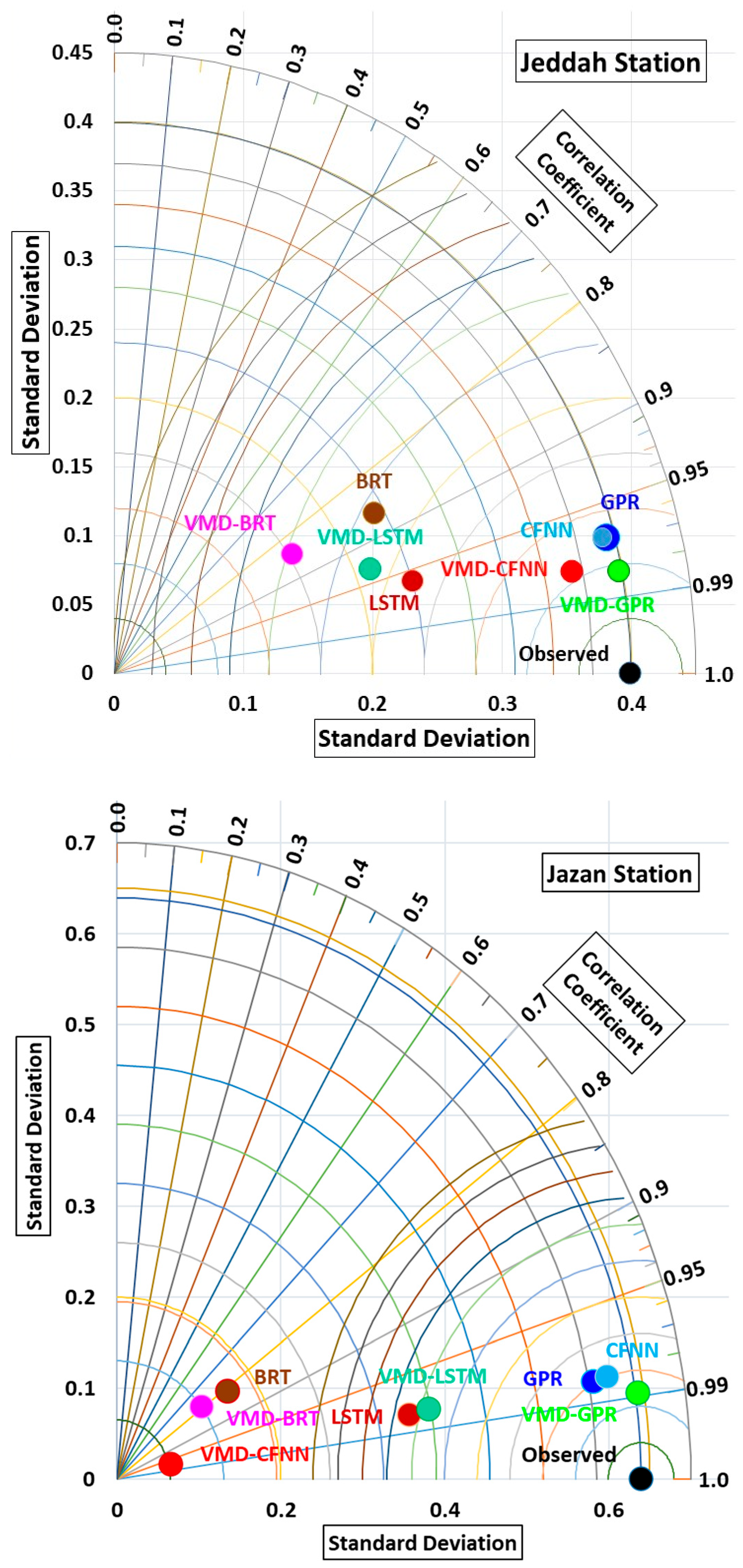
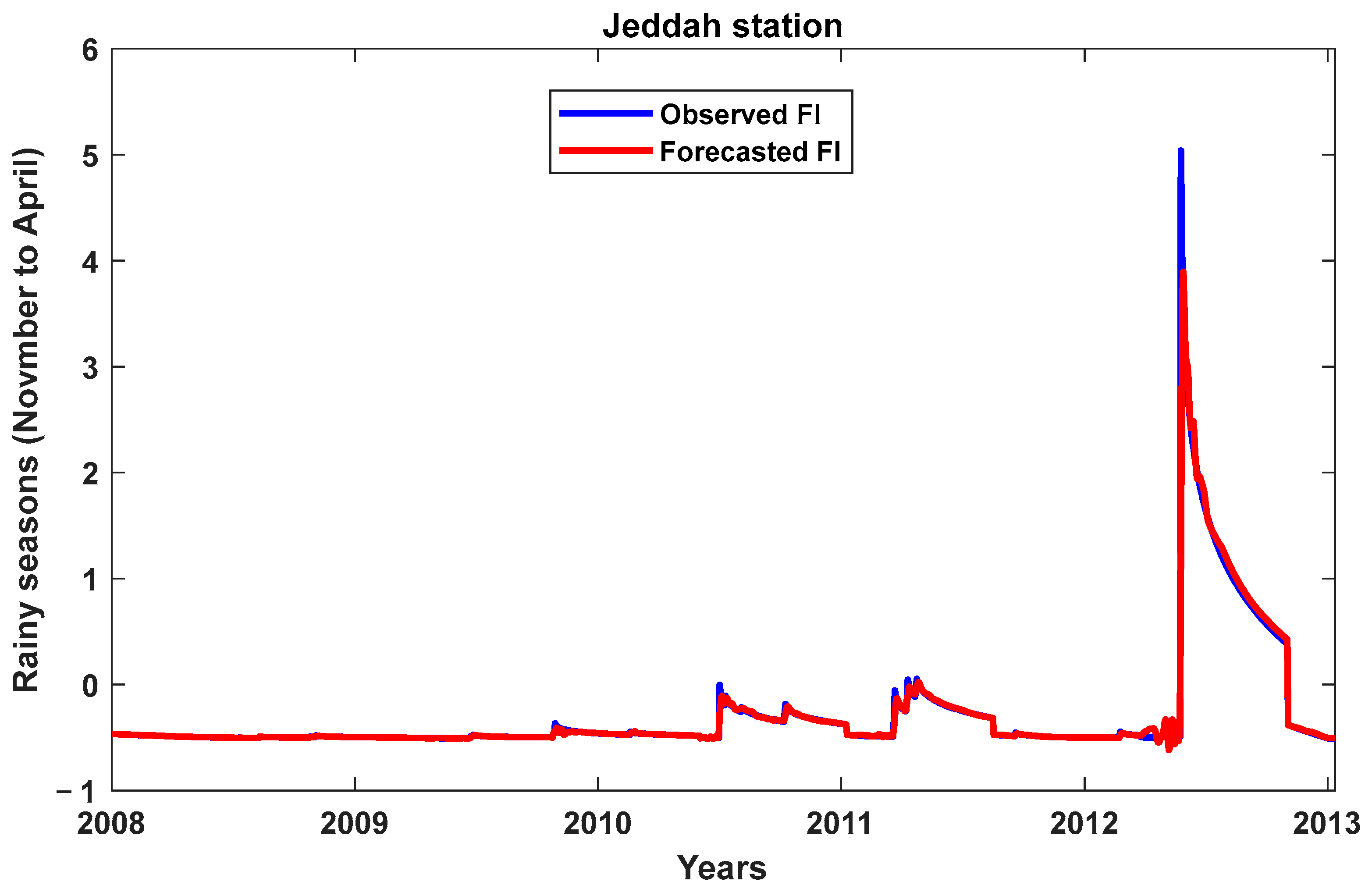
3. Results and Discussion
4. Conclusions
Author Contributions
Funding
Data Availability Statement
Acknowledgments
Conflicts of Interest
References
- Wu, W.; Emerton, R.; Duan, Q.; Wood, W.A.; Wetterhall, F.; Robertson, E.D. Ensemble flood forecasting: Current status and future opportunities. Wiley Interdiscip. Rev. Water 2020, 7, e1432. [Google Scholar] [CrossRef]
- Hou, S.; Wei, J.; Hou, M.; Xu, J.; Han, L. A hydrological knowledge-informed LSTM model for monthly streamflow reconstruction using distributed data: Application to typical rivers across the Tibetan plateau. J. Hydrol. 2025, 649, 132409. [Google Scholar] [CrossRef]
- Baig, M.B.; Alotibi, Y.; Straquadine, S.G.; Alataway, A. Water resources in the Kingdom of Saudi Arabia: Challenges and strategies for improvement. In Water Policies in MENA Countries; Springer: Cham, Switzerland, 2020; pp. 135–160. [Google Scholar]
- Erica DeNicola, E.; Aburizaiza, S.O.; Siddique, A.; Khwaja, H.; Carpenter, O.D. Climate change and water scarcity: The case of Saudi Arabia. Ann. Glob. Health 2015, 81, 342–353. [Google Scholar] [CrossRef] [PubMed]
- Almazroui, M. Rainfall trends and extremes in Saudi Arabia in recent decades. Atmosphere 2020, 11, 964. [Google Scholar] [CrossRef]
- Nevo, S.; Morin, E.; Rosenthal, G.A.; Metzger, A.; Barshai, C.; Weitzner, D.; Voloshin, D.; Kratzert, F.; Elidan, G.; Gideon Dror, G.; et al. Flood forecasting with machine learning models in an operational framework. Hydrol. Earth Syst. Sci. 2022, 26, 4013–4032. [Google Scholar] [CrossRef]
- Noymanee, J.; Theeramunkong, T. Flood forecasting with machine learning technique on hydrological modeling. Procedia Comput. Sci. 2019, 156, 377–386. [Google Scholar] [CrossRef]
- Motta, M.; de Castro Neto, M.; Sarmento, P. A mixed approach for urban flood prediction using Machine Learning and GIS. Int. J. Disaster Risk Reduct. 2021, 56, 102154. [Google Scholar] [CrossRef]
- Rajab, A.; Farman, A.; Islam, N.; Syed, D.; Elmagzoub, A.; Shaikh, A.; Akram, M.; Alrizq, A. Flood forecasting by using machine learning: A study leveraging historic climatic records of Bangladesh. Water 2023, 15, 3970. [Google Scholar] [CrossRef]
- Shafizadeh-Moghadam, H.; Valavi, R.; Shahabi, H.; Chapi, K.; Shirzadi, A. Novel forecasting approaches using combination of machine learning and statistical models for flood susceptibility mapping. J. Environ. Manag. 2018, 217, 1–11. [Google Scholar] [CrossRef]
- Sankaranarayanan, S.; Sahoo, A.; Satapathy, D.P. Flood prediction based on weather parameters using deep learning. J. Water Clim. Chang. 2020, 11, 1766–1783. [Google Scholar] [CrossRef]
- Prasad, R.; Deo, R.C. Weekly soil moisture forecasting with multivariate sequential, ensemble empirical mode decomposition and Boruta-random forest hybridizer algorithm approach. Catena 2019, 177, 149–166. [Google Scholar] [CrossRef]
- Soman, K.P.; Athira, S.; Harikumar, K. Recursive Variational Mode Decomposition Algorithm for Real Time Power Signal Decomposition. Procedia Technol. 2015, 21, 540–546. [Google Scholar] [CrossRef]
- Mallat, S.G. A Wavelet Tour of Signal Processing; Academic: New York, NY, USA, 1998. [Google Scholar]
- Mallat, S.G. A theory for multiresolution signal decomposition: The wavelet representation. IEEE Trans. Pattern Anal. Mach. Intell. 1989, 11, 674–693. [Google Scholar] [CrossRef]
- Nourani, V.; Aida Hosseini Baghanam, H.A.; Adamowski, J.; Kisi, O. Applications of hybrid wavelet–Artificial Intelligence models in hydrology: A review. J. Hydrol. 2014, 514, 358–377. [Google Scholar] [CrossRef]
- Nourani, V.; Komasi, M.; Mano, A. A multivariate ANN-wavelet approach for rainfall–runoff modeling. Water Resour. Manag. 2009, 23, 2877–2894. [Google Scholar] [CrossRef]
- Deo, R.C.; Tiwari, M.K.; Adamowski, J.F.; Quilty, J.M. Forecasting effective drought index using a wavelet extreme learning machine (W-ELM) model. Stoch. Environ. Res. Risk Assess. 2016, 31, 1211–1240. [Google Scholar] [CrossRef]
- Deo, R.C.; Wen, X.; Qi, F. A wavelet-coupled support vector machine model for forecasting global incident solar radiation using limited meteorological dataset. Appl. Energy 2016, 168, 568–593. [Google Scholar] [CrossRef]
- Krishna, B.; Rao, Y.R.S.; Nayak, P.C. Time Series Modeling of River Flow Using Wavelet Neural Networks. J. Water Resour. Prot. 2011, 03, 50–59. [Google Scholar] [CrossRef]
- Huang, N.E.; Shen, Z.; Long, S.R.; Wu, M.C.; Shih, H.H.; Zheng, Q.; Yen, N.; Tung, C.C.; Liu, H.H. The empirical mode decomposition and the Hilbert spectrum for nonlinear and non-stationary time series analysis. Proc. R. Soc. A 1998, 454, 903–995. [Google Scholar] [CrossRef]
- Wu, Z.; Huang, N.E. Ensemble empirical mode decomposition: A noise-assisted data analysis method. Adv. Adapt. Data Anal. 2009, 1, 1–41. [Google Scholar] [CrossRef]
- Torres, M.E.; Colominas, M.A.; Schlotthauer, G.; Flandrin, F. A complete ensemble empirical mode decomposition with adaptive noise. In Proceedings of the 2011 IEEE International Conference on Acoustics, Speech and Signal Processing (ICASSP), Prague, Czech Republic, 22–27 May 2011. [Google Scholar]
- Colominas, M.A.; Schlotthauer, G.; Torres, M.E. Improved complete ensemble EMD: A suitable tool for biomedical signal processing. Biomed. Signal Process. Control 2014, 14, 19–29. [Google Scholar] [CrossRef]
- Ali, M.; Deo, R.C.; Maraseni, T.; Downs, N.J. Improving SPI-derived drought forecasts incorporating synoptic-scale climate indices in multi-phase multivariate empirical mode decomposition model hybridized with simulated annealing and kernel ridge regression algorithms. J. Hydrol. 2019, 576, 164–184. [Google Scholar] [CrossRef]
- Ali, M.; Prasad, R. Significant wave height forecasting via an extreme learning machine model integrated with improved complete ensemble empirical mode decomposition. Renew. Sustain. Energy Rev. 2019, 104, 281–295. [Google Scholar] [CrossRef]
- Dragomiretskiy, K.; Zosso, D. Variational Mode Decomposition. IEEE Trans. Signal Process. 2014, 62, 531–544. [Google Scholar] [CrossRef]
- Fu, T.; Li, X.; Jia, R.; Feng, L. A novel integrated method based on a machine learning model for estimating evapotranspiration in dryland. J. Hydrol. 2021, 603, 126881. [Google Scholar] [CrossRef]
- Wang, D.; Liu, Y.; Luo, H.; Yue, C.; Cheng, S. Day-ahead PM2. 5 concentration forecasting using WT-VMD based decomposition method and back propagation neural network improved by differential evolution. Int. J. Environ. Res. Public Health 2017, 14, 764. [Google Scholar] [CrossRef]
- Zhou, J.; Sun, N.; Jia, B.; Peng, T. A novel decomposition-optimization model for short-term wind speed forecasting. Energies 2018, 11, 1752. [Google Scholar] [CrossRef]
- Majumder, I.; Dash, P.; Bisoi, R. Variational mode decomposition based low rank robust kernel extreme learning machine for solar irradiation forecasting. Energy Convers. Manag. 2018, 171, 787–806. [Google Scholar] [CrossRef]
- Moishin, M.; Deo, R.C.; Prasad, R.; Raj, N.; Abdulla, S. Development of Flood Monitoring Index for daily flood risk evaluation: Case studies in Fiji. Stoch. Environ. Res. Risk Assess. 2021, 35, 1387–1402. [Google Scholar] [CrossRef]
- Williams, C.; Rasmussen, C. Gaussian processes for regression. In Advances in Neural Information Processing Systems; MIT Press: Cambridge, MA, USA, 1995; Volume 8. [Google Scholar]
- Gao, J.; Ling, H.; Hu, W.; Xing, J. Transfer learning based visual tracking with gaussian processes regression. In Proceedings of the Computer Vision–ECCV 2014: 13th European Conference, Zurich, Switzerland, 6–12 September 2014. [Google Scholar]
- Williams, C.K.; Rasmussen, C.E. Gaussian Processes for Machine Learning; MIT Press: Cambridge, MA, USA, 2006; Volume 2. [Google Scholar]
- Ghasemi, P.; Karbasi, M.; Nouri, A.Z.; Tabrizi, M.S.; Azamathulla, H.M. Application of Gaussian process regression to forecast multi-step ahead SPEI drought index. Alex. Eng. J. 2021, 60, 5375–5392. [Google Scholar] [CrossRef]
- Yu, Y.; Si, X.; Hu, C.; Zhang, J. A review of recurrent neural networks: LSTM cells and network architectures. Neural Comput. 2019, 31, 1235–1270. [Google Scholar] [PubMed]
- Staudemeyer, R.C.; Morris, E.R. Understanding LSTM—A tutorial into long short-term memory recurrent neural networks. arXiv 2019, arXiv:1909.09586. [Google Scholar]
- Sherstinsky, A. Fundamentals of recurrent neural network (RNN) and long short-term memory (LSTM) network. Phys. D Nonlinear Phenom. 2020, 404, 132306. [Google Scholar] [CrossRef]
- Friedman, J.H. Greedy function approximation: A gradient boosting machine. Ann. Stat. 2001, 29, 1189–1232. [Google Scholar] [CrossRef]
- Saha, S.; Arabameri, A.; Saha, A.; Blaschke, T.; Ngo, P.T.T.; Nhu, V.H.; Band, S.S. Prediction of landslide susceptibility in Rudraprayag, India using novel ensemble of conditional probability and boosted regression tree-based on cross-validation method. Sci. Total Environ. 2021, 764, 142928. [Google Scholar] [CrossRef]
- Faskari, S.A.; Falope, T.; Ojim, G.; Abdullahi, U.B.; Abba, S.I. A Novel Machine Learning based Computing Algorithm in Modeling of Soiled Photovoltaic Module. Knowl.-Based Eng. Sci. 2022, 3, 28–36. [Google Scholar]
- Elith, J.; Leathwick, J.R.; Hastie, T. A working guide to boosted regression trees. J. Anim. Ecol. 2008, 77, 802–813. [Google Scholar] [CrossRef]
- Naghibi, S.A.; Pourghasemi, H.R. A comparative assessment between three machine learning models and their performance comparison by bivariate and multivariate statistical methods in groundwater potential mapping. Water Resour. Manag. 2015, 29, 5217–5236. [Google Scholar]
- Carty, D.M.; Young, T.M.; Zaretzki, R.L.; Guess, F.M.; Petutschnigg, A. Predicting and correlating the strength properties of wood composite process parameters by use of boosted regression tree models. For. Prod. J. 2015, 65, 365–371. [Google Scholar]
- Westreich, D.; Lessler, J.; Funk, M.J. Propensity score estimation: Neural networks, support vector machines, decision trees (CART), and meta-classifiers as alternatives to logistic regression. J. Clin. Epidemiol. 2010, 63, 826–833. [Google Scholar]
- Fahlman, S.; Lebiere, C. The cascade-correlation learning architecture. In Advances in Neural Information Processing Systems; MIT Press: Cambridge, MA, USA, 1989; Volume 2. [Google Scholar]
- Dharma, S.; Hassan, M.H.; Ong, H.C.; Sebayang, A.H.; Silitonga, A.S.; Kusumo, F.; Milano, J. Experimental study and prediction of the performance and exhaust emissions of mixed Jatropha curcas-Ceiba pentandra biodiesel blends in diesel engine using artificial neural networks. J. Clean. Prod. 2017, 164, 618–633. [Google Scholar] [CrossRef]
- Mohammadi, M.-R.; Hemmati-Sarapardeh, A.; Schaffie, M.; Husein, M.M.; Ranjbar, M. Application of cascade forward neural network and group method of data handling to modeling crude oil pyrolysis during thermal enhanced oil recovery. J. Pet. Sci. Eng. 2021, 205, 108836. [Google Scholar] [CrossRef]
- Willmott, C.J. Some comments on the evaluation of model performance. Bull. Am. Meteorol. Soc. 1982, 63, 1309–1313. [Google Scholar] [CrossRef]
- McCuen, R.H.; Knight, Z.; Cutter, A.G. Evaluation of the Nash–Sutcliffe efficiency index. J. Hydrol. Eng. 2006, 11, 597–602. [Google Scholar] [CrossRef]
- Gupta, H.V.; Kling, H.; Yilmaz, K.K.; Martinez, G.F. Decomposition of the mean squared error and NSE performance criteria: Implications for improving hydrological modelling. J. Hydrol. 2009, 377, 80–91. [Google Scholar] [CrossRef]
- Fijani, E.; Barzegar, R.; Deo, R.C.; Tziritis, E.; Skordas, K. Design and implementation of a hybrid model based on two-layer decomposition method coupled with extreme learning machines to support real-time environmental monitoring of water quality parameters. Sci. Total Environ. 2019, 648, 839–853. [Google Scholar] [CrossRef]
- Shamseldin, A.Y. Application of a neural network technique to rainfall runoff. J. Hydrol. 1997, 199, 272–294. [Google Scholar] [CrossRef]
- Xu, Z.; Hou, Z.; Han, Y.; Guo, W. A diagram for evaluating multiple aspects of model performance in simulating vector fields. Geosci. Model Dev. 2016, 9, 4365–4380. [Google Scholar] [CrossRef]
- Sloughter, J.M.; Gneiting, T.; Raftery, A.E. Probabilistic wind speed forecasting using ensembles and Bayesian model averaging. J. Am. Stat. Assoc. 2010, 105, 25–35. [Google Scholar] [CrossRef]
- Tiwari, M.K.; Chatterjee, C. A new wavelet–bootstrap–ANN hybrid model for daily discharge forecasting. J. Hydroinform. 2011, 13, 500–519. [Google Scholar] [CrossRef]
- Gao, F.; Shao, X. A novel interval decomposition ensemble model for interval carbon price forecasting. Energy 2022, 243, 123006. [Google Scholar] [CrossRef]


| Stations | Models | Tuning Parameters |
|---|---|---|
| Jeddah Station | GPR | Hybrid and Standalone Structure
|
| LSTM |
| |
| BRT |
| |
| CFNN |
| |
| Jazan Station | GPR | Hybrid and Standalone Structure
|
| LSTM |
| |
| BRT |
| |
| CFNN |
|
| Jeddah Station | Jazan Station | |||||
|---|---|---|---|---|---|---|
| r | RMSE | MAE | r | RMSE | MAE | |
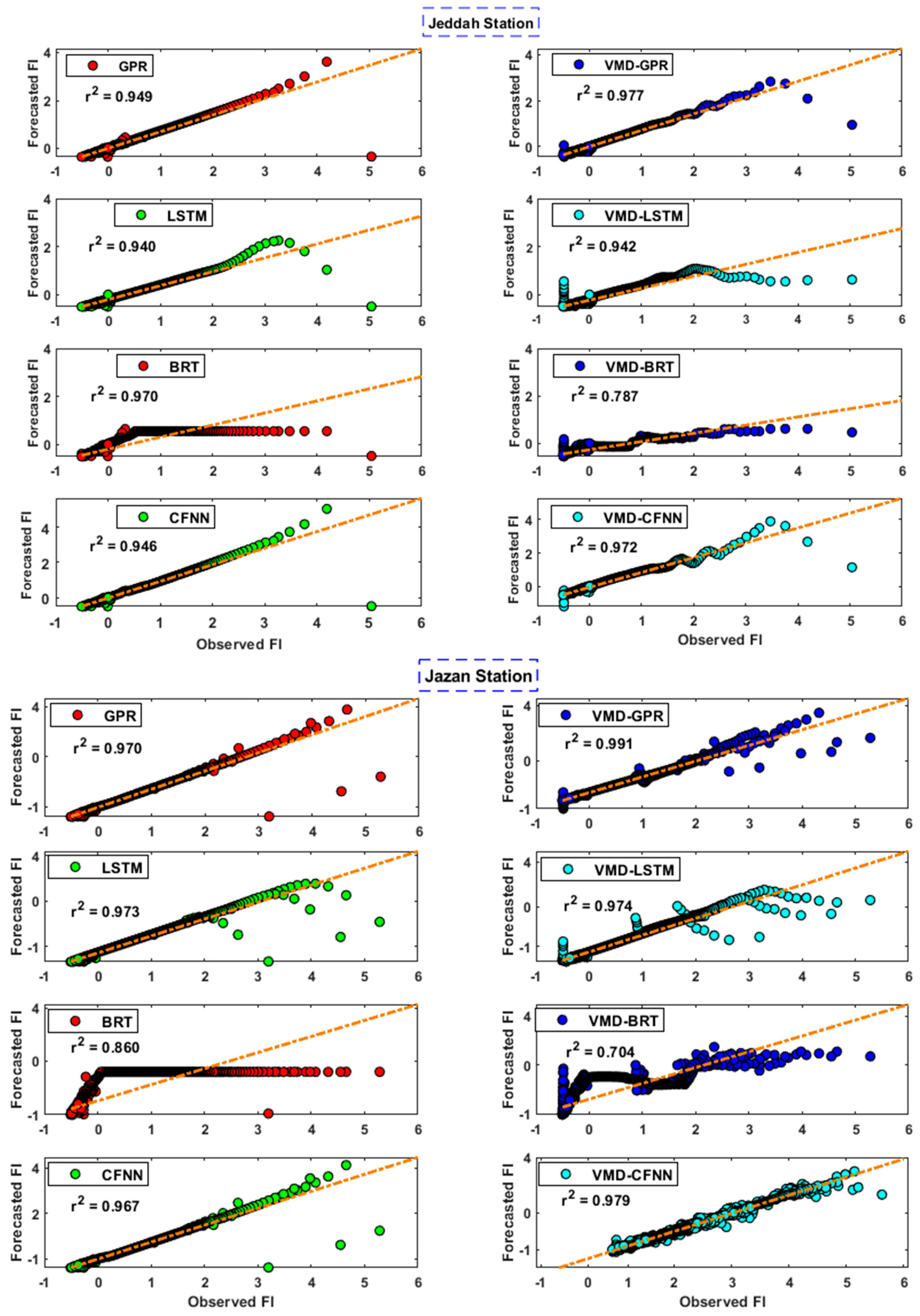
| GPR | 0.9678 | 0.1006 | 0.0051 | 0.9834 | 0.1227 | 0.0179 |
| VMD-GPR | 0.9825 | 0.0745 | 0.0088 | 0.9891 | 0.0945 | 0.0189 |
| LSTM | 0.9603 | 0.1902 | 0.0588 | 0.9809 | 0.3126 | 0.1140 |
| VMD-LSTM | 0.9348 | 0.2213 | 0.0655 | 0.9802 | 0.2895 | 0.1098 |
| BRT | 0.8661 | 0.2316 | 0.0330 | 0.8164 | 0.5311 | 0.1416 |
| VMD-BRT | 0.8485 | 0.2787 | 0.0700 | 0.7943 | 0.5625 | 0.1636 |
| CFNN | 0.9674 | 0.1012 | 0.0062 | 0.9827 | 0.1205 | 0.0156 |
| VMD-CFNN | 0.9788 | 0.0870 | 0.0109 | 0.9726 | 0.1349 | 0.0187 |
| Jeddah Station | Jazan Station | |||||||
|---|---|---|---|---|---|---|---|---|
| ENS | KGE | IA | U95% | ENS | KGE | IA | U95% | |
| GPR | 0.9364 | 0.9646 | 0.9836 | 0.2790 | 0.9631 | 0.9003 | 0.9899 | 0.3390 |
| VMD-GPR | 0.9651 | 0.9802 | 0.9911 | 0.2065 | 0.9781 | 0.9849 | 0.9945 | 0.2621 |
| LSTM | 0.7731 | 0.5690 | 0.9111 | 0.5146 | 0.7608 | 0.3483 | 0.9034 | 0.8372 |
| VMD-LSTM | 0.6927 | 0.5034 | 0.8665 | 0.6043 | 0.7948 | 0.3995 | 0.9208 | 0.7753 |
| BRT | 0.6636 | 0.5529 | 0.8573 | 0.6393 | 0.3098 | 0.0339 | 0.5521 | 1.4471 |
| VMD-BRT | 0.5129 | 0.3757 | 0.7420 | 0.7677 | 0.2257 | −0.0480 | 0.4559 | 1.5308 |
| CFNN | 0.9357 | 0.9598 | 0.9833 | 0.2806 | 0.9644 | 0.9285 | 0.9905 | 0.3332 |
| VMD-CFNN | 0.9525 | 0.9019 | 0.9867 | 0.2409 | 0.9455 | 0.9690 | 0.9861 | 0.3740 |
Disclaimer/Publisher’s Note: The statements, opinions and data contained in all publications are solely those of the individual author(s) and contributor(s) and not of MDPI and/or the editor(s). MDPI and/or the editor(s) disclaim responsibility for any injury to people or property resulting from any ideas, methods, instructions or products referred to in the content. |
© 2025 by the authors. Licensee MDPI, Basel, Switzerland. This article is an open access article distributed under the terms and conditions of the Creative Commons Attribution (CC BY) license (https://creativecommons.org/licenses/by/4.0/).
Share and Cite
Aldhafiri, A.A.; Ali, M.; Labban, A.H. Leveraging Advanced Data-Driven Approaches to Forecast Daily Floods Based on Rainfall for Proactive Prevention Strategies in Saudi Arabia. Water 2025, 17, 1699. https://doi.org/10.3390/w17111699
Aldhafiri AA, Ali M, Labban AH. Leveraging Advanced Data-Driven Approaches to Forecast Daily Floods Based on Rainfall for Proactive Prevention Strategies in Saudi Arabia. Water. 2025; 17(11):1699. https://doi.org/10.3390/w17111699
Chicago/Turabian StyleAldhafiri, Anwar Ali, Mumtaz Ali, and Abdulhaleem H. Labban. 2025. "Leveraging Advanced Data-Driven Approaches to Forecast Daily Floods Based on Rainfall for Proactive Prevention Strategies in Saudi Arabia" Water 17, no. 11: 1699. https://doi.org/10.3390/w17111699
APA StyleAldhafiri, A. A., Ali, M., & Labban, A. H. (2025). Leveraging Advanced Data-Driven Approaches to Forecast Daily Floods Based on Rainfall for Proactive Prevention Strategies in Saudi Arabia. Water, 17(11), 1699. https://doi.org/10.3390/w17111699