Heavy Rainfall Probabilistic Model for Zielona Góra in Poland

Abstract

The research focuses on probabilistic modeling of maximum rainfall in Zielona Góra, Poland, to improve urban drainage system design. The study utilizes archived pluviographic data from 1951 to 2020, collected at the IMWM-NRI meteorological station. These data include 10 min rainfall records and aggregated hourly and daily totals. The study employs various statistical distributions, including Fréchet, gamma, generalized exponential (GED), Gumbel, log-normal, and Weibull, to model rainfall intensity–duration–frequency (IDF) relationships. After testing the goodness of fit using the Anderson–Darling test, Bayesian Information Criterion (BIC), and relative residual mean square Error (rRMSE), the GED distribution was found to best describe rainfall patterns. A key outcome is the development of a new rainfall model based on the GED distribution, allowing for the estimation of precipitation amounts for different durations and exceedance probabilities. However, the study highlights limitations, such as the need for more accurate local models and a standardized rainfall atlas for Poland.

1. Introduction

The design and sizing of urban and rural drainage systems are primarily based on the analysis of maximum anticipated rainfall events. Precipitation models, which describe the relationship between rainfall height (h, mm), event duration (t, min), and exceedance probability (p), provide the fundamental basis for this process. Depending on the intended application, rainfall height can be expressed in terms of rainfall intensity (I, mm/min) or unit runoff (q, dm³/s·ha) [1,2].

Contemporary regulations stipulate that the dimensioning of sewer systems must rely on the best available technical knowledge (BAT) and account for the anticipated impacts of climate change. According to the European Standard EN 752 (2008) [3], sewer flooding events should occur only with rare and socially acceptable frequencies: once every 10 years for rural areas and once every 20 to 50 years for urban areas, depending on land use characteristics (Table 1).

In cases involving the expansion or modernization of existing systems, the application of BAT principles now necessitates the use of advanced hydrodynamic simulation tools [2,4,5,6]. Such tools are increasingly indispensable in engineering practice, enabling performance assessments of stormwater drainage and combined sewer systems, as well as associated structures such as stormwater overflows caused by obstructed drains [7,8,9,10], separators, and retention reservoirs [6,11,12,13]. In parallel, considerable research attention has recently been devoted to the assessment of risks related to urban infrastructure [14,15,16,17,18,19] and the impacts of climate change on the functioning of drainage systems [20,21,22,23,24,25]. Moreover, the type of precipitation has been recognized as a key factor influencing the selection of drainage technologies and the mitigation of landslide risks associated with water erosion [26].

Table 1. Recommended frequency of designed computational rain to limit the incidence of spills in accordance to PN-EN 752 [27].

Class	Description Due to Land Use	Frequency of Design Rainfall Occurrence [1 per C Years]	Probability p [%]	Frequency of Outflow Occurrence [1 per C Years]	Probability p [%]
I	Non-urban (rural) areas	1 per 1	1	1 per 10	10
II	Residential areas	1 per 2	50	1 per 20	5
III	City centers and service and industrial areas	1 per 5	20	1 per 30	3.33
IV	Underground communication facilities, passages and crossings under streets, etc.	1 per 10	10	1 per 50	2

Table 1. Recommended frequency of designed computational rain to limit the incidence of spills in accordance to PN-EN 752 [27].

Class	Description Due to Land Use	Frequency of Design Rainfall Occurrence [1 per C Years]	Probability p [%]	Frequency of Outflow Occurrence [1 per C Years]	Probability p [%]
I	Non-urban (rural) areas	1 per 1	1	1 per 10	10
II	Residential areas	1 per 2	50	1 per 20	5
III	City centers and service and industrial areas	1 per 5	20	1 per 30	3.33
IV	Underground communication facilities, passages and crossings under streets, etc.	1 per 10	10	1 per 50	2

A persistent challenge in the design of drainage systems remains the limited availability of reliable maximum rainfall models for urban areas. Germany has successfully addressed this issue with the development of the KOSTRA atlas, which provides reference rainfall intensities for individual urban basins. Analogous efforts were initiated earlier in the United States [28]. In Poland, however, by 2020, detailed maximum rainfall models with specified durations and exceedance probabilities had been developed only for selected cities, including Wroclaw, Lublin, Krakow, Lodz, and Czestochowa [28,29,30,31,32,33]. In most other areas, designers must rely on national-scale models, whose applicability is limited due to substantial spatial variability in precipitation patterns [34].

The primary obstacle to the development of local rainfall models in Poland has been the limited availability of long-term, high-resolution pluviographic data. Although the Institute of Meteorology and Water Management–National Research Institute (IMWM-PIB) has collected rainfall data for many decades, systematic digital recording commenced only relatively recently [35]. Consequently, much of the historical rainfall data exist solely as paper records, the manual processing of which is labor intensive, particularly for specific rainfall durations [29].

Significant improvements in data availability have occurred since 2020 with the publication of the Polish Atlas of Reliable Intensities (PANDa) and, subsequently, the Maximum Precipitation Atlas (PMAXTP) developed by IMWM-NRI in 2022 [36,37,38]. For the construction of a reliable maximum rainfall model suitable for drainage system design and simulation—particularly for C values ranging from 1 to 50 years—a minimum of 50 years of continuous rainfall records is recommended. In some cases, 30 years of records may suffice with appropriate extrapolation, although shorter series may fail to capture the full natural variability of extreme rainfall events [38,39].

The aforementioned atlases were developed based on rainfall records from the period 1986–2015, spanning 30 years. In the present study, the authors seek to compare the publicly available PMAXTP atlas data with a locally developed point rainfall model for the city of Zielona Góra, where high-resolution precipitation records covering a 70-year period (1951–2020) are available. Verifying and updating the PMAXTP atlas is crucial, considering its widespread application in drainage system modeling and in the preparation of water-law permit applications across Poland [9].

Recent advances in statistical rainfall modeling have significantly enhanced the methodology of distribution fitting, offering a valuable reference framework for the development and validation of local intensity–duration–frequency (IDF) models. A notable example is the study by Montes-Pajuelo et al. [40], which presented a comprehensive evaluation of ten probability distributions for modeling 24 h annual maximum precipitation. The assessed distributions included exponential, normal, two- and three-parameter log-normal, gamma, Gumbel, log-Gumbel, Pearson type III, log-Pearson type III, and SQRT-ET max. The results indicated that the log-Gumbel and three-parameter log-normal distributions offered superior performance for high return periods, whereas Gumbel and log-normal models provided better accuracy for lower return periods. These findings emphasize the importance of selecting appropriate statistical formulations based on the specific characteristics of the precipitation regime under consideration.

Further research has explored the use of more flexible four-parameter distributions. For instance, the Kappa distribution (K4D) has been shown to be particularly effective in modeling extreme daily precipitation based on annual maxima, as demonstrated in a recent study by [41]. This suggests that higher-parameter models may offer improved representation of tail behavior and extremes, often under-represented by classical two-parameter formulations.

On a regional scale, Min-Seop et al. [42] proposed new evaluation frameworks aimed at improving the assessment of precipitation distributions, particularly within the context of CMIP5 and CMIP6 climate model outputs. Their analyses identified common deficiencies in simulated rainfall data, including systematic overestimation of light precipitation and underestimation of heavy rainfall events. These discrepancies underscore the necessity of refining distribution fitting techniques to better represent spatial and temporal variabilities in precipitation, especially for regional hydrological applications.

Moreover, recent modeling efforts have begun to address the statistical challenges associated with zero inflation and the high frequency of dry days in daily rainfall series. A noteworthy development is the introduction of an extended Pareto distribution with zero inflation, designed to capture dry spells, typical wet-day events, and extremes within a unified framework [43]. This approach, which incorporates covariate effects through generalized additive models, enhances the capacity to represent climate-induced variability in rainfall occurrence and intensity.

2. Materials and Methods

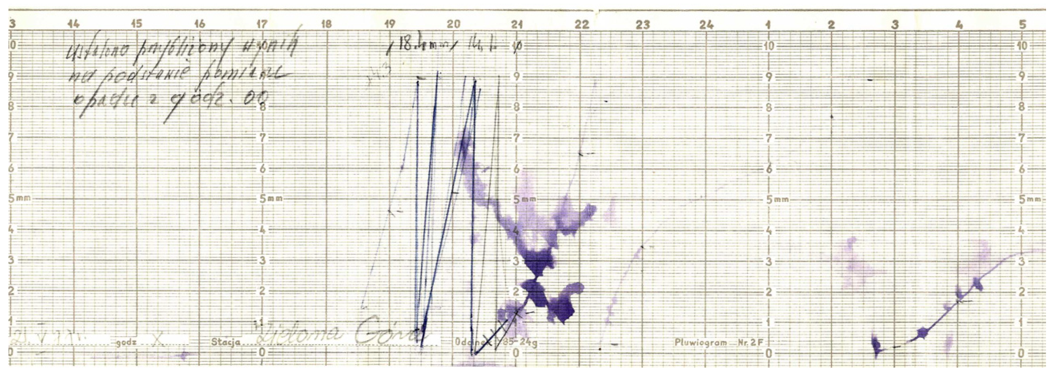
2.1. Heavy Rainfall Records

The present investigation utilizes archived pluviograph records from the Institute of Meteorology and Water Management–National Research Institute (IMWM-NRI) meteorological station in Zielona Góra, encompassing the period 1951–2020. These instrumentation-derived data quantify heavy rainfall intensities at ten-minute resolutions and have been systematically aggregated into hourly and daily precipitation totals for subsequent analysis. Figure 1 presents a high-resolution scan of the original paper precipitation strip, which constituted the primary source of gauge data until its digitization in the early 2000s. The exceptional temporal continuity and resolution of this dataset enable robust detection of extreme pluviometric events and facilitate comprehensive trend analysis over seven decades. Consequently, these records represent a critical resource for advancing our understanding of long-term hydrometeorological variability.

The measuring station in Zielona Góra, as part of a national measurement and observation network at the hydrological and meteorological service, is a synoptic station that is participating in an international program to monitor weather (Weather World Watch) as part of the World Meteorological Organization (WMO), of which Poland is a member. The station building is located on the south-eastern outskirts of the city of Zielona Góra at an altitude of 108 m above sea level. Physiographicly Zielona Góra is situated temporarily on the south of Lubusz voivodeship in the basin of the Odra river in Poland. The predominant land use in both the municipality and around the station are fields and wasteland [6].

As part of the national measurement program, the station in Zielona Góra utilizes standard synoptic station equipment, comprising meteorological instruments connected to an automated MAWS workstation [44,45]. Precipitation measurements are performed concurrently using an automatic SEBA rain gauge, which records data at 10 min intervals, and by a meteorological observer employing a traditional Hellmann rain gauge. Observations are conducted at six-hour intervals, with daily totals also recorded. Data from both methods are systematically compared and verified following each measurement session to ensure accuracy. Since the launch of the automatic station network in 1999, digital precipitation data have been archived in the IMWM-NRI database. Prior to this period, continuous precipitation records were maintained using paper strips in clockwork-operated pluviographs, devices that had been operating in Poland continuously since the 1960s. The standard pluviograph provided a continuous trace of rainfall events over the course of a day, mapped onto a 10 min grid with an ordinate resolution of 1 mm. At the end of each day (at 6 UTC), the pluviograph strip was replaced, and the recorded data were analyzed and summarized in a “pluviographic summary”, which documented two key values: the total daily precipitation and the cumulative duration of rainfall episodes.

In order to ensure many years of measurement sequences and establish appropriate digital-to-analog solutions, despite the official withdrawal of the measuring device from IMWM-NRI, measurements using pluviograph were held in Zielona Góra up to 2020, which made it possible to build a rare and extremely valuable in terms of quality and accuracy of comparative rainfall measurements strings [45,46]. The systematic development of archival rainfall data derived exclusively from float-type rain gauges played a crucial role in preserving the genetic homogeneity of the time series. National studies consistently emphasize that the introduction of automatic rain gauges into measurement sequences often results in significant disturbances to data homogeneity [29,47,48]. In order to present the climatological background of rainfall variability in Zielona Góra, the results section presents the range of variability of annual rainfall sums, the relationship between the cold and warm half-years during the year, the average monthly values from the multi-year period, and the annual variability of the highest annual values in the analyzed period.

2.2. Probabilistic Models

The maximum precipitation model developed as a probabilistic model was based on a common statistical procedure used, e.g., by Kotowski and Kaźmierczak for Wrocław [1,49] and by Wdowikowski for the Odra river basin [39,44], and this method was also the basis for the development of the PANDa and PMAXTP atlases and was described in detail [37,38].

In order to establish the empirical linkage between observed precipitation depths, event durations, and their corresponding exceedance probabilities, we first delineated the subset of archival pluviograph records to be used for intensity–duration–frequency (IDF) analysis. Drawing upon a comprehensive study of 63 Polish meteorological stations over the 1951–1990 interval—where the most extreme daily rainfall depths were shown to concentrate in the May–October (V–X) period, while winter maxima (November–April) were both infrequent and below the long-term mean of annual extremes [35]—we confined our analysis to heavy-rainfall events occurring between May and October. This seasonal restriction minimizes the influence of low-magnitude winter storms on the upper tail of the depth–duration distribution. Using a total-review approach, we investigated the entire archive for the target months and isolated the fifty highest precipitation depths (h) for each of twenty discrete durations (t), as follows:

• Minutes: 5, 10, 20, 30, 40, and 50;
• Hours: 1, 1.5, 2, 3, 6, 12, and 18;
• Days: 1, 1.5, 2, 3, 4, 5, and 6.

This dense grid of extreme-event observations across sub-hourly to multi-day scales provides a high-resolution dataset ideally suited for urban catchment design and hydrological modeling. Within each duration class, the fifty maxima were rank ordered in descending magnitude and then assigned empirical exceedance probabilities according to the plotting-position formula in Equation (1). The largest event in each class corresponds to p = 0.020, while the smallest corresponds to p = 0.980, thereby enabling the construction of robust empirical IDF curves for subsequent design and risk-assessment applications.

$$p(m,n)={\displaystyle \frac{m}{n+1}}$$

(1)

Here, m stands for the sequence number within an n power-decreasing ordered string.

To describe the measurement data, we used theoretical distributions: Fréchet, gamma, generalized exponential (GED), Gumbel, log-normal, and Weibull [25,44,50,51,52,53,54,55,56,57].

Table 2. Log-likelihood function for the particular distributions.

Distribution (Number of Parameters)	Likelihood Function
Fréchet (3)	$\mathrm{l}\mathrm{n}L={\alpha }^n{\beta }^{n\alpha }{\displaystyle \prod _{i=1}^n}{\left(x_i-\gamma \right)}^{-\left(\alpha +1\right)}\mathrm{e}\mathrm{x}\mathrm{p}\left[-{\displaystyle \sum _{i=1}^n}{\left({\displaystyle \frac{\beta }{x_i-\gamma }}\right)}^{\alpha }\right]$
Gamma (3)	$\mathrm{l}\mathrm{n}L=\left(\alpha -1\right){\displaystyle \sum _{i=1}^n}\mathrm{l}\mathrm{n}\left(x_i-\gamma \right)-n\mathrm{l}\mathrm{n}\Gamma \left(\alpha \right)-na\mathrm{l}\mathrm{n}\beta -{\displaystyle \frac{1}{\beta }}{\displaystyle \sum _{i=1}^n}\left(x_i-\gamma \right)$
GED (3)	$\mathrm{l}\mathrm{n}L=n\mathrm{l}\mathrm{n}\alpha +n\mathrm{l}\mathrm{n}\lambda -{\displaystyle \sum _{i=1}^n}\left(\lambda \left(x_i-\gamma \right)\right)+\left(\alpha -1\right){\displaystyle \sum _{i=1}^n}\mathrm{l}\mathrm{n}\left(1-e^{-\left(x_i-\mu \right)\lambda }\right)$
Gumbel (2)	$\mathrm{l}\mathrm{n}L=-n\mathrm{l}\mathrm{n}\sigma -{\displaystyle \sum _{i=1}^n}\left({\displaystyle \frac{x_i-\gamma }{\sigma }}\right)-{\displaystyle \sum _{i=1}^n}\mathrm{e}\mathrm{x}\mathrm{p}\left(-{\displaystyle \frac{x_i-\gamma }{\sigma }}\right)$
Log-normal (3)	$\mathrm{l}\mathrm{n}L=-{\displaystyle \sum _{i=1}^n}\mathrm{l}\mathrm{n}\left(x_i-\gamma \right)-n\mathrm{l}\mathrm{n}\sigma -{\displaystyle \frac{n}{2}}\mathrm{l}\mathrm{n}\left(2\pi \right)-{\displaystyle \frac{1}{2{\sigma }^2}}{\displaystyle \sum _{i=1}^n}{\left(\mathrm{l}\mathrm{n}\left(x_i-\gamma \right)-\mu \right)}^2$
Weibull (3)	$\mathrm{l}\mathrm{n}L=n\mathrm{l}\mathrm{n}\alpha -n\alpha \mathrm{l}\mathrm{n}\beta +\left(\alpha -1\right){\displaystyle \sum _{i=1}^n}\mathrm{l}\mathrm{n}\left(x_i-\gamma \right)-{\displaystyle \sum _{i=1}^n}{\left({\displaystyle \frac{x_i-\gamma }{\beta }}\right)}^{\alpha }$

presents the likelihood functions for each selected distribution, where α, β, γ, λ, and μ denote the respective distributional parameters. Parameter estimation was performed via the maximum likelihood method (MLM), employing numerical optimization of the likelihood (or log-likelihood) function within specified parameter bounds to ensure convergence to the global optimum [58,59].

The goodness of fit between the theoretical models and the observed data was assessed using the Anderson–Darling statistic, following the procedures outlined in [49,60,61]:

$$A^2=-n-{\displaystyle \frac{1}{n}}\sum _{i=1}^n\left(2i-1\right)\left[\mathrm{l}\mathrm{n}F\left(X_i\right)+\mathrm{l}\mathrm{n}\left(1-F\left(X_{n-i+1}\right)\right)\right]$$

(2)

where X_i—is the i-th value in the decreasing ordered random sample;

F(X)—the cumulative distribution function for the reference distribution.

To assess the suitability of each candidate distribution, we formulated the null hypothesis H₀ that the sample data follow the distribution in question. This hypothesis was tested at the 5% significance level (α = 0.05), specifically, H₀ was retained if the Anderson–Darling statistic $A^2$ did not exceed its critical threshold $A_{crit}^2$. Conversely, if $A^2>A_{crit}^2$, the alternative hypothesis H_A —that the data deviate from the assumed distribution—was accepted. Critical values for $A^2$ were obtained from established statistical tables [49,60,62].

After excluding the Gumbel distribution due to its poor goodness of fit, the remaining contenders were compared using the Bayesian Information Criterion (BIC) of Schwarz [20,63,64], defined as:

$$BIC=-{\displaystyle \frac{2\mathrm{l}\mathrm{n}L}{n}}+{\displaystyle \frac{k\mathrm{l}\mathrm{n}n}{n}}$$

(3)

where L is the maximized likelihood, k the number of estimated parameters, and n is the sample size. This criterion balances model complexity against fit quality, enabling selection of the most parsimonious distribution.

The Bayesian Information Criterion (BIC) comprises two terms: the first quantifies the goodness of fit of the model, while the second imposes a penalty for model complexity. The distribution yielding the lowest BIC value is deemed the most parsimonious yet adequately descriptive. To further assess the fidelity of each candidate distribution to the observed data, we also employed the relative root mean square error (rRMSE) [49,65]:

$$rRMSE=\sqrt{{\displaystyle \frac{1}{n}}\sum _{i=1}^n{\left({\displaystyle \frac{h_{o,i}-h_{p,i}}{h_{p,i}}}\right)}^2}·100\%$$

(4)

where h_o—the amount of precipitation from calculations (mm);

h_p—the amount of precipitation from measurements (mm).

The quantile function Q(p) of a random variable specifies the value x such that the cumulative distribution function F(x) equals a given probability p. For the generalized error distribution (GED), this function explicitly incorporates the distribution’s shape, scale, and location parameters to map p ∈ (0, 1) to the corresponding quantile. In closed form, the GED quantile function is, therefore, expressed as follows:

$$h(p)=\gamma -{\displaystyle \frac{1}{\lambda }}\ln \left(1-{\left(1-p\right)}^{{\displaystyle \frac{1}{\alpha }}}\right)$$

(5)

and, thus, random variables are created, which can be generated based on the above formula for any frequency or probability of occurrence. The consistency of measurement data with the model-generated maximum precipitation values can be presented on an h–h plot or q–q plot, where h stands for the rainfall height in [mm], and q stands for the quantile, also in [mm].

3. Results

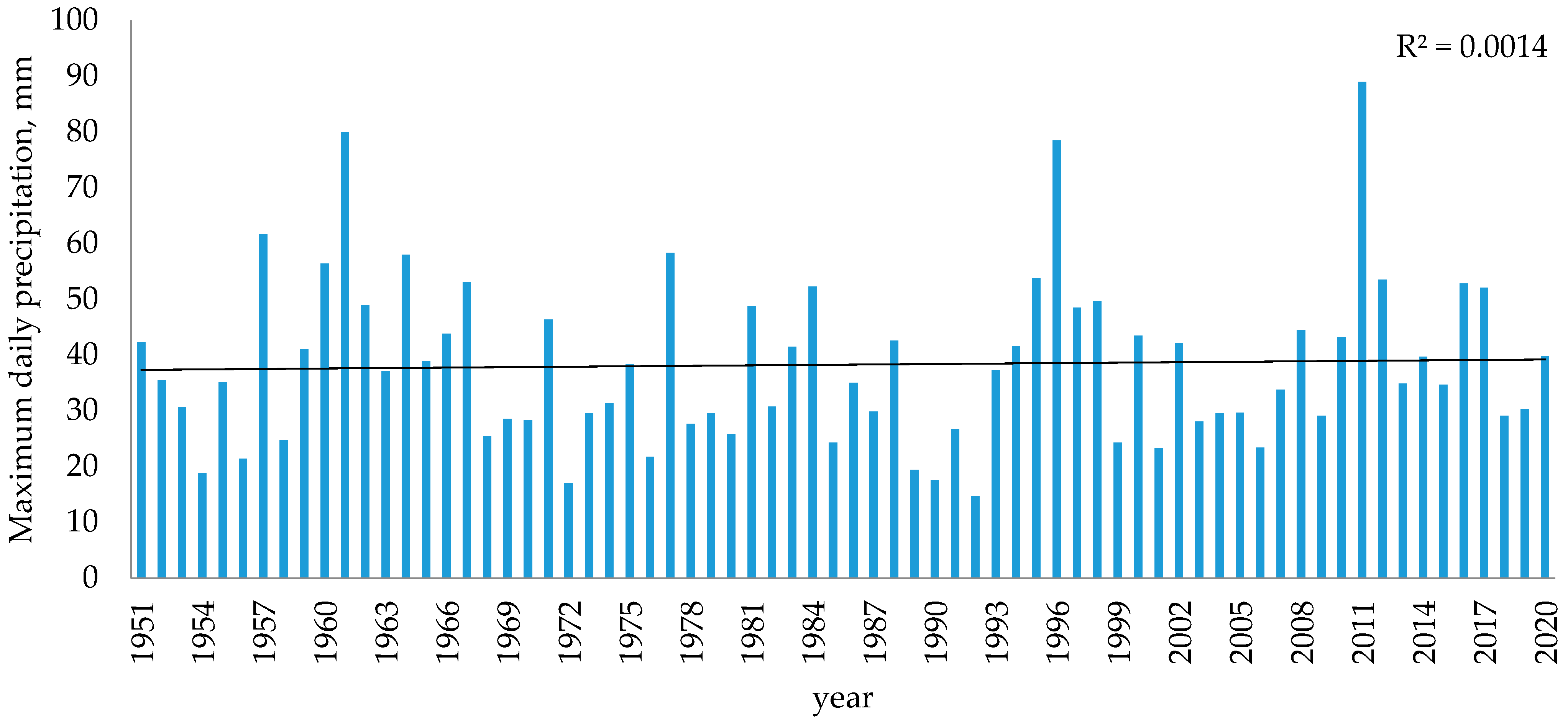
3.1. Climatological Background

In Zielona Góra, within the analyzed period of 70 years, we recorded 12,002 days with a precipitation amount exceeding 0.1 mm, which is the limit of precipitation measurement accuracy. In the course of a long-term period, the total rainy days was in the range from 120 to 191 which gives the percentage of 32.9% to 52.3% for the year, and in the analysis of the warm half-years (which contains the months May to October), the number of days of rainfall was in the range 57–94. The percentage of the entire year of rainy days in the warm period was from 15.6% to 25.8% and from 47.5% to 49.2% with respect to rainy days of the year (Figure 2). The average number of all the days of the analyzed wet period is 161 (44% of the year). Within the summer half-year, there are, on average, 76 wet days, representing 20.8% of the entire year and 47.4% of the total number of wet days, as illustrated in Figure 3.

Annual totals in Zielona Góra varied and ranged from 384 mm (in 1982) to 807 mm (2017). The long-term average for the period 1951–2020 was 587 mm. The contribution of precipitation during the summer half-year (May–October) to the annual total ranged between 53.9% and 82.5%, reflecting the characteristic precipitation patterns of the Lubusz Voivodeship, with a pronounced concentration during the summer months. The highest monthly precipitation totals typically occurred in the summer season, with July most frequently recording the maximum values (

Table 3. The maximum, minimum, and average monthly rainfall totals in the long-term period of 1951–2020.

Month	Maximum Monthly Rainfall, mm	Minimum Monthly Rainfall, mm	Average Monthly Rainfall, mm
I	107.2	2.0	40.3
II	93.0	2.4	33.3
III	129.9	8.1	38.2
IV	81.4	1.7	37.7
V	132.8	8.7	55.0
VI	143.5	8.5	59.4
VII	219.3	6.0	80.9
VIII	196.4	6.9	68.4
IX	144.4	1.1	46.3
X	162.4	2.9	41.5
XI	123.3	0.8	41.7
XII	114.8	5.0	43.9

).

The maximum daily totals recorded t the station varied from 14.7 mm (in 2007) to 89.0 mm (in 2001), while the heaviest day totals in the summer season V–X of the long-term period from 1951 to 2020. There is a statistically insignificant linear change trend detected in the analyzed period, with an R² coefficient equal to 0.0014. The variability in maximum daily precipitation totals is shown in Figure 4.

A comprehensive analysis of the pluviographic records used in the researched 70 years indicates an increase in the incidence of maximum daily precipitation amounts despite the declining value of annual precipitation totals and the annual number of days with precipitation. In Zielona Góra, exceptionally high daily precipitation values were typically associated with short-duration rainfall events. The observed long-term changes, particularly the increase in intense rainfall events in recent years, underscore a concerning trend and highlight the growing importance of studies focused on the probabilistic characterization of meteorological phenomena.

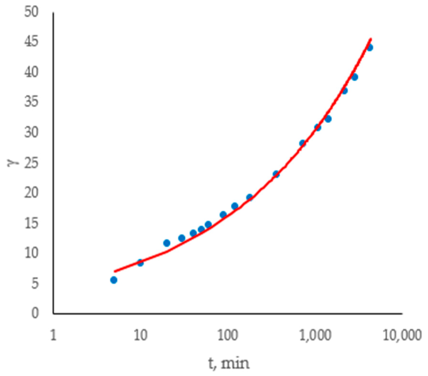
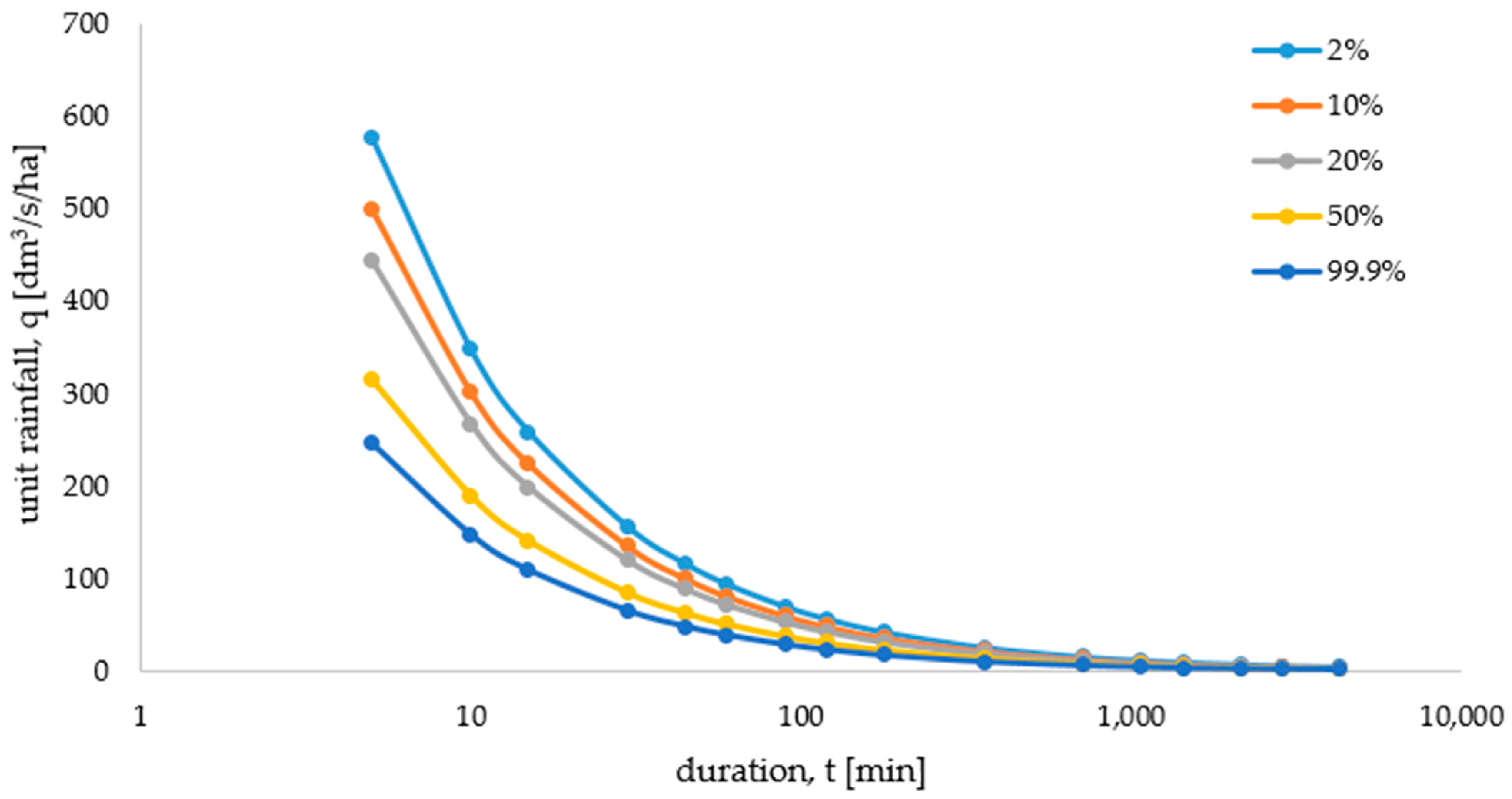
3.2. Zielona Góra Maximum Precipitation Probabilistic Model

Based on the procedure for developing a probabilistic model of maximum precipitation described in Chapter 2, measurement data were prepared and processed, and then a statistical precipitation model for Zielona Góra was constructed and validated.

It should be emphasized that the highest estimation errors in probability analyses are typically associated with the extreme values of the examined data series: in this case, maximum precipitation events [44,66,67,68,69,70].

Table 4. Measured amounts of precipitation for the selected empirical probability values.

t, min	m = 1 p = 0.020	m = 5 p = 0.098	m = 10 p = 0.196	m = 25 p = 0.490	m = 50 p = 0.980
	mm	mm	mm	mm	mm
5	13.6	10.1	8.9	7.1	5.6
10	19.2	14.4	12.3	10.5	8.5
20	30.1	23.3	17.4	13.9	11.6
30	37.9	25.2	19.6	15.6	12.5
40	39.9	27.7	22.0	16.5	13.3
50	40.6	27.7	22.7	17.6	13.9
60	41.8	33.0	26.3	18.5	14.8
90	45.1	38.0	26.3	19.8	16.3
120	45.9	38.0	28.1	22.4	17.8
180	51.9	38.9	33.4	24.7	19.2
360	55.0	43.8	37.7	27.6	23.1
720	56.9	49.7	41.1	35.7	28.1
1080	73.6	55.7	49.3	39.7	30.9
1440	89.1	60.6	55.0	41.1	32.3
2160	96.0	68.8	61.0	46.6	36.9
2880	103.5	72.1	63.3	51.6	39.2
4320	109.6	77.1	68.0	57.0	44.1

presents the recorded precipitation amounts corresponding to the selected empirical probability values.

The results of the MLM estimation of parameters are summarized in

Table 5. Values of the parameter estimates (according to MLM).

t, min		GED	Weibull	LogN	Fréchet	Gumbel	Gamma
5	α	1.2073	1.2218	0.8047	1.1158	2.8022	1.1974
	β	0.5373	6.9021	0.5524	2.1726	2.8019	1.7482
	γ	5.588		5.336	5.593	3.887	5.589
10	α	0.934	1.4506	0.7255	1.1155	3.6127	1.1751
	β	0.3835	10.0798	0.8429	2.6083	4.5195	2.1422
	γ	8.499		8.014	8.485	5.357	8.479
20	α	0.8478	2.4935	1.0529	0.898	1.5692	0.8506
	β	0.2291	13.7787	0.8868	3.71	2.4516	4.5979
	γ	11.599		11.432	11.599	10.667	11.599
30	α	0.828	3.0051	1.0079	0.8971	1.9607	0.8329
	β	0.1833	15.2481	1.1671	4.5722	4.179	5.7783
	γ	12.499		12.172	12.499	10.378	12.499
40	α	0.6898	3.4532	1.0405	0.8176	1.8469	0.6995
	β	0.1445	16.3324	1.2689	4.8956	4.4391	7.7066
	γ	13.299		12.897	13.299	11.065	13.299
50	α	0.6259	3.8474	1.0765	0.7734	1.6968	0.6359
	β	0.1232	17.209	1.3334	5.2324	4.4171	9.302
	γ	13.899		13.497	13.899	11.805	13.899
60	α	0.7971	4.0984	1.1353	0.8748	1.379	0.8045
	β	0.1373	18.2752	1.3024	5.8697	3.4332	7.7877
	γ	14.799		14.594	14.799	13.63	14.799
90	α	0.508	4.302	1.3958	0.6597	1.2201	0.516
	β	0.1005	19.5611	1.1018	4.9403	2.9965	12.0712
	γ	16.299		16.131	16.299	15.181	16.299
120	α	0.678	4.441	1.1378	0.8105	1.5574	0.6887
	β	0.1142	21.5927	1.4142	6.117	4.5909	9.8078
	γ	17.799		17.454	17.799	15.775	17.799
180	α	0.7391	4.871	1.1002	0.8511	1.7216	0.7496
	β	0.1092	23.4419	1.5583	6.947	5.8069	9.991
	γ	19.199		18.754	19.199	16.39	19.199
360	α	0.7853	4.8504	0.981	0.884	1.9674	0.7949
	β	0.1106	27.5004	1.6845	7.2844	6.8062	9.6907
	γ	23.099		22.438	23.099	19.605	23.099
720	α	0.9482	5.1145	0.7429	1.0834	3.5905	0.9625
	β	0.1116	33.5368	2.0793	8.9322	15.8564	9.0007
	γ	28.099		26.407	28.079	16.966	28.099
1080	α	1.2541	6.1379	0.6378	1.1797	4.9274	1.2749
	β	0.1061	37.7856	2.426	11.3887	27.3413	8.5104
	γ	30.752		27.841	30.783	9.801	30.732
1440	α	1.1821	7.0333	0.7759	1.1033	3.0399	1.1734
	β	0.0916	39.8475	2.3453	12.5417	17.7746	10.3342
	γ	32.239		30.489	32.266	20.934	32.242
2160	α	0.7879	8.751	1.0153	0.8997	1.9386	0.8
	β	0.0625	44.9462	2.2479	13.0911	12.4994	17.1124
	γ	36.899		35.843	36.899	30.372	36.899
2880	α	0.8456	9.5142	0.8784	0.9531	3.0244	0.859
	β	0.0585	48.5409	2.5137	15.0585	24.0482	17.8585
	γ	39.199		37.16	39.199	22.938	39.199
4320	α	0.9199	9.0368	0.694	1.0791	3.8322	0.9335
	β	0.0606	53.9953	2.7247	16.1135	30.142	16.7588
	γ	44.099		40.491	44.06	22.648	44.099

.

Table 6. A² statistic values for analyzed distributions.

t, min	Fréchet	Gamma	GED	Gumbel	Log-Normal	Weibull
5	0.287	0.114	0.115	0.695	0.201	0.120
10	0.398	0.383	0.951	0.592	0.350	0.368
20	0.254	0.503	0.514	2.169	0.207	0.458
30	0.308	0.423	0.427	1.524	0.313	0.401
40	0.207	0.541	0.538	1.448	0.206	0.525
50	0.293	0.835	0.828	1.601	0.243	0.845
60	0.431	0.352	0.359	2.032	0.272	0.319
90	0.541	0.759	0.743	2.113	0.537	0.964
120	0.426	0.392	0.392	1.573	0.320	0.388
180	0.422	0.285	0.285	1.556	0.383	0.291
360	0.392	0.688	0.693	2.182	0.444	0.660
720	0.344	0.587	0.611	0.631	0.318	0.315
1080	0.239	0.314	0.699	0.445	0.213	0.275
1440	0.284	0.266	0.268	0.861	0.258	0.273
2160	0.514	0.292	0.295	1.101	0.406	0.272
2880	0.545	0.508	0.515	0.628	0.575	0.449
4320	0.287	0.959	0.985	0.579	0.279	0.521
A2crit	0.757	0.762	0.723	0.757	0.752	0.757

shows the calculated results for the A² statistic. For improved clarity, A² values lower than the critical threshold have been highlighted in bold.

Two of the analyzed distributions, i.e., Fréchet and log-normal distributions, fulfilled the criterion evaluated for each of the 20 analyzed rainfall duration intervals. Gamma and Weibull distributions, found only in 2 cases, and GED distributions, occurring in 3 of the 17 cases, did not conform to the specified criteria. Therefore, we concluded that the measurement data certainly do not fit the Gumbel distribution.

BIC values for the analyzed distributions are summarized in

Table 7. BIC values of analyzed distributions.

t, min	Fréchet	Gamma	GED	Log-Normal	Weibull
5	203.02	199.40	199.36	201.54	199.38
10	240.50	228.44	228.28	237.28	229.66
20	276.14	251.04	250.58	271.24	255.42
30	287.38	272.58	272.34	282.98	274.20
40	299.92	289.36	289.24	296.18	289.86
50	303.58	295.20	295.14	300.38	295.38
60	309.08	303.02	303.00	307.08	302.60
90	312.30	303.32	303.16	309.62	304.38
120	312.44	306.56	306.50	309.80	306.80
180	327.50	316.30	316.20	323.58	316.88
360	339.42	329.12	329.00	351.54	329.68
720	348.72	340.70	340.62	361.34	341.20
1080	355.64	346.66	346.58	367.32	346.98
1440	375.40	368.20	368.08	373.66	368.52
2160	390.50	378.82	378.70	386.38	379.60
2880	404.30	393.42	393.30	400.72	394.20
4320	433.02	404.46	404.46	410.28	8.4031

. For the sake of clarity, the smallest values are bolded (for each duration t).

The BIC criterion results (Table 7) demonstrate that the GED distribution attains the lowest BIC for all seventeen rainfall durations considered, establishing it as the most parsimonious model overall. However, the narrow gaps in BIC scores among GED, gamma, and Weibull highlight the near-equivalent performances of these three distributions.

An rRMSE statistics review (

Table 8. rRMSE values of analyzed distributions.

t, min	Gamma	GED	Weibull
5	1.87	1.83	2.00
10	2.41	2.88	2.50
20	3.94	4.01	3.67
30	4.23	4.30	4.00
40	3.02	3.11	2.63
50	3.44	3.45	3.36
60	3.69	3.72	3.60
90	3.61	3.56	4.47
120	2.96	2.93	3.10
180	3.02	3.02	3.03
360	3.86	3.87	3.83
720	2.89	2.93	2.50
1080	2.26	2.34	2.23
1440	3.25	3.24	3.30
2160	2.39	2.38	2.34
2880	3.33	3.35	3.02
4320	3.50	3.55	3.11

) revealed that Weibull distribution achieved the minimum values in eleven of the seventeen cases and appeared as the best-fitted distribution. The GED distribution outperformed only in five of the seventeen rainfall intervals, and the gamma model emerged as the best-fitting distribution only for two durations, t = 10 and t = 180 min (the smallest values for all best rainfall durations are bolded and underlined).

An inspection of the rRMSE values in Table 8 also reveals distinct performance regimes for the three candidate distributions across the full range of rainfall durations (5 min to 4320 min). At the shortest intervals (5–10 min), the GED and gamma models attain the lowest errors—indicative of their capacity to capture rapid, high-intensity bursts—whereas the Weibull model lags slightly. For intermediate durations (20–60 min) and most multi-hour to multi-day scales (360–4320 min), the Weibull distribution consistently yields the smallest rRMSE, underscoring its robustness in characterizing longer-term accumulations. The GED regains competitive accuracy around the 90–120 min window and again at the 1440 min (one-day) duration, reflecting its flexibility across diverse temporal resolutions.

When aggregated over all seventeen durations, the Weibull distribution achieves the lowest overall rRMSE (3.099%), followed closely by gamma (3.157%) and GED (3.204%), with the margins between them remaining very small. By contrast, the log-normal (4.718%), Fréchet (5.548%), and Gumbel (6.892%) distributions exhibit substantially larger errors, confirming their relatively poorer agreement with the measured data.

Taken together with the BIC rankings (Table 7), these rRMSE results reinforce the GED as the most reliable single model for the Zielona Góra precipitation record. The duration-dependent GED parameter estimates are plotted in the h–h diagram of Figure 5, illustrating the distribution’s uniform performance from sub-hourly to multi-day time scales.

Figure 5 illustrates that the pluviograph records from Zielona Góra are accurately characterized by the GED. However, the original formulation of model (5) requires distinct parameter sets for each discrete rainfall duration (Table 5), which complicates its use in engineering applications and precludes estimation for unlisted durations (e.g., 15 or 45 min). To overcome these limitations, we derived a unified precipitation–duration–exceedance relationship applicable for any t ϵ [5; 4320] min and p ϵ (0.02; 1]. Notably, the shape parameter α exhibited negligible variation across durations; hence, we adopted its mean value (ᾱ = 0.947) and subsequently re-estimated the scale λ and dispersion γ parameters under this constraint. The resulting parameter values are summarized in

Table 9. GED distribution parameters for rainfall duration.

t, min	α	λ	γ
5	0.947	0.2766	4.59
10		0.2766	8.29
20		0.1980	11.29
30		0.1753	12.49
40		0.1531	12.99
50		0.1454	13.69
60		0.1454	13.69
90		0.1323	16.49
120		0.1294	18.19
180		0.1165	19.99
360		0.1036	23.89
720		0.0924	28.59
1080		0.0872	32.39
1440		0.0746	35.69
2160		0.0628	38.69
2880		0.0491	41.29
4320		0.0447	41.29

, providing a continuous formulation that facilitates interpolation for arbitrary durations within the analyzed range.

Leveraging the GED parameter estimates listed in Table 9, we constructed a series of diagnostic plots (Figure 6 and Figure 7) to examine how each distributional parameter evolves across the full spectrum of rainfall durations. These visualizations not only reveal the relative stability of the shape parameter but also highlight systematic trends in the scale and dispersion estimates, thereby guiding the interpolation strategy for intermediate durations.

Empirical regression of the GED parameters against event duration t (in minutes) yielded power-law relationships of the form

$$\lambda =1.567t^{-0.281},\hspace{1em}\hspace{1em}{R}^2=0.97$$

(6)

$$\gamma =4.596t^{0.274},\hspace{1em}\hspace{1em}{R}^2=0.96$$

(7)

Here, $R^2$ denotes the coefficient of determination for each fit, indicating excellent explanatory power of the proposed functions over the full range t ϵ [5; 4320]. Substituting (6) and (7) into the GED quantile formulation produces a continuous model for precipitation depth h as a function of duration t and exceedance probability p:

$$h(p,t)=4.596t^{0.274}-1.567t^{0.281}\ln \left(1-{\left(1-p\right)}^{1.063}\right)$$

(8)

where the exponent 1.063 corresponds to the fixed shape parameter α. Figure 8 presents the h–h plot comparing observed and predicted quantiles, confirming the high fidelity of Equation (8) in reproducing the Zielona Góra rainfall record.

A comparison of the quantile predictions from models (5) and (8) reveals notable divergences at both extremes of the rainfall spectrum. For multi-day events yielding depths in excess of 100 mm, model (8) systematically underpredicts the upper quantiles relative to the duration-specific parameterizations of model (5) (Table 5). Similarly, for light-to-moderate events (rainfall depths ≤ 20 mm), model (8) exhibits modest bias compared to the more finely tuned fits of model (5). Despite these discrepancies, the closed-form simplicity of Equation (8) renders it highly practical for rapid sizing of urban drainage infrastructure and for generalized precipitation–frequency analyses.

4. Comparison of the Regional Model with the PMAXTP Atlas

Maximum precipitation data from the PMAXTP atlas for comparative analysis for Zielona Góra were downloaded from the public domain of IMWM-NRI: klimat.imgw.pl. The results of reliable maximum precipitation for durations from 5 min to 4320 min in [mm] and the selected probabilities are included in

Table 10. Maximum precipitation values from PMAXTP atlas.

t, Duration	Probability of Occurrence, p
	1%	2%	5%	10%	20%	33%	50%	99.9%
5	19.14	17.29	14.94	13.25	11.60	10.45	9.44	7.35
10	22.99	20.80	18.01	15.97	13.98	12.57	11.34	8.78
15	25.59	23.17	20.08	17.82	15.59	14.01	12.62	9.75
30	30.73	27.87	24.20	21.48	18.79	16.87	15.17	11.65
45	34.20	31.06	26.99	23.97	20.96	18.80	16.88	12.93
60	36.90	33.53	29.17	25.90	22.64	20.30	18.22	13.93
90	41.07	37.36	32.53	28.90	25.26	22.62	20.28	15.46
120	44.32	40.34	35.15	31.23	27.29	24.43	21.89	16.65
180	49.32	44.95	39.20	34.84	30.44	27.23	24.37	18.48
360	59.23	54.07	47.24	42.01	36.68	32.78	29.27	22.09
720	71.13	65.05	56.92	50.65	44.21	39.45	35.16	26.40
1080	79.17	72.48	63.48	56.51	49.30	43.97	39.15	29.30
1440	85.42	78.26	68.59	61.07	53.27	47.48	42.24	31.55
2160	95.07	87.20	76.50	68.13	59.42	52.92	47.03	35.02
2880	102.58	94.15	82.66	73.63	64.20	57.15	50.75	37.71
4320	114.17	104.90	92.19	82.14	71.61	63.70	56.49	41.86

, and the intensity–duration–frequency curves are shown in the Figure 9.

To compare the maximum precipitation values for the probabilistic regional model for Zielona Góra with the PMAXTP atlas, quantile values were generated from the model given by the Formula (8) and are presented in Figure 10 for the main frequencies of design rainfall occurrence C mentioned in Table 1, as well as compared using relative residuals, as shown in

Table 11. Comparison of maximum precipitation [mm] between PMAXTP and regional model for Zielona Góra.

t, Duration	Probability of Occurrence, p
	1%	2%	5%	10%	20%	33%	50%	99.9%
5	−0.84	−0.69	−0.83	−0.54	−0.55	−0.60	−0.74	−0.25
10	−0.79	−0.60	−0.85	−0.61	−0.57	−0.68	−0.74	−0.18
15	−0.69	−0.57	−0.89	−0.58	−0.62	−0.69	−0.82	−0.05
30	−0.53	−0.47	−0.94	−0.60	−0.68	−0.79	−0.87	0.05
45	−0.40	−0.46	−0.95	−0.49	−0.67	−0.86	−0.88	0.07
60	−0.30	−0.33	−0.89	−0.47	−0.70	−0.84	−0.92	0.17
90	−0.07	−0.26	−0.82	−0.43	−0.70	−0.86	−0.88	0.34
120	0.08	−0.14	−0.84	−0.45	−0.63	−0.89	−0.89	0.45
180	0.38	0.05	−0.70	−0.30	−0.64	−0.84	−0.87	0.62
360	1.07	0.53	−0.55	−0.14	−0.61	−0.88	−0.87	1.01
720	1.97	1.15	−0.27	0.18	−0.45	−0.81	−0.76	1.50
1080	2.63	1.62	−0.03	0.42	−0.31	−0.80	−0.75	1.90
1440	3.28	2.04	0.18	0.61	−0.17	−0.77	−0.64	2.15
2160	4.23	2.70	0.59	1.00	−0.03	−0.72	−0.53	2.68
2880	4.92	3.25	0.88	1.24	0.07	−0.60	−0.45	3.09
4320	6.23	4.10	1.35	1.71	0.36	−0.41	−0.19	3.74

. In Figure 10, it can be observed that for the example values of probabilities p = 1, 5 and 50% of maximum precipitation occurrence, the results are comparable.

Table 11 shows that the greatest difference concerns the lowest probability of maximum rainfall occurrence, i.e., the rarest values; then, the largest difference is 6 mm, and the vast majority of observed differences do not exceed 1 mm, which basically leads to the conclusion that the models are comparable, and it does not matter whether the data were taken from 30 years, i.e., the period 1986–2015 at PMAXTP, or from 70 for the regional model, i.e., the years 1951–2020.

5. Discussion

In this study, probabilistic modeling of maximum rainfall in Zielona Góra was performed using a unique 70-year archival pluviograph record (1951–2020), which enabled an assessment of parameter stability in comparison to the PMAXTP atlas model based on a 30-year period (1986–2015) [37,38]. The primary objective was to identify the statistical distribution that most accurately captures the relationship between rainfall depth, duration, and exceedance probability and then to derive a simplified formulation suitable for engineering practice without necessitating individual calibration of parameters for each duration. This work builds upon the approaches of Kotowski and Kaźmierczak [1,56] and Wdowikowski et al. [39,44] and follows established recommendations for developing local intensity–duration–frequency (IDF) models in Poland [71].

Six candidate distributions—Fréchet, gamma, generalized exponential (GED), Gumbel, log-normal, and Weibull—were fitted to the series of annual maxima for 20 distinct durations (5 min to 6 days) using maximum likelihood estimation. The goodness of fit was evaluated via the Anderson–Darling test at a significance level of 0.05 [60,66]. The Gumbel distribution was rejected outright, as its test statistic exceeded the critical threshold for all durations, whereas Fréchet and log-normal met the criterion across every interval. Model selection was then guided by the Bayesian Information Criterion (BIC), which imposes a stronger penalty on model complexity than the Akaike criterion [20], and by the relative root mean square error (rRMSE) [65]. Although Weibull yielded the lowest aggregate rRMSE (3.10%), the GED distribution consistently achieved the lowest BIC values and offered a compelling balance between parsimony and fit (rRMSE = 3.20%) [44,56].

To enhance practical usability, the standard GED quantile function given by Formula (5), which would normally require distinct parameters (α, λ, γ) for each duration, was reformulated to the simple pattern given in (8), where parameter ᾱ = 0.947 is the duration-averaged shape parameter, and λ(t) and γ(t) are power-law functions (t) that are duration dependent, with coefficients of determination R ≃ 0.97 and 0.96, respectively. This unified expression covers all t ∈ [5, 4320] min and p ∈ (0.02, 1] without recourse to tabulated parameter sets [39,72].

A comparison with PMAXTP values from the IMWM-NRI database, using identical durations and exceedance probabilities (1%, 2%, 5%, 10%, 20%, 33%, 50%, and 99.9%), revealed that for design-relevant thresholds (5–20%), the relative differences between the regional model and the atlas data remained below 1 mm, an amount considered negligible from an engineering standpoint. Larger discrepancies, reaching up to 6.2 mm, were observed only for rare events with a 1% exceedance probability and extended durations of up to 3 days. These findings indicate that despite the PMAXTP atlas being based on a shorter 30-year data record, its spatial interpolation and methodological consistency produce IDF estimates that are effectively comparable to those derived from a longer, locally consistent dataset [38].

Nonetheless, the regional model’s reliance on a single, consistently recorded pluviograph series [36,47] may better capture site-specific extremes, whereas the atlas model’s multi-station interpolation smooths local idiosyncrasies [6,46]. To further enhance probabilistic descriptions of extremes, future research should focus on data quality control during the transition from mechanical pluviographs to automated gauges [30,48], the exploration of alternative estimation frameworks such as L-moments or Bayesian inference [25,63], and the development of non-stationary or non-linear models to account for ongoing climatic shifts [64,65]. These advances will provide engineers with more robust tools to design drainage infrastructure that remains resilient under evolving extreme rainfall regimes.

In the study, six statistical distributions were applied—including five three-parameter models: log-normal, Weibull, gamma, GED, and Fréchet—to model extreme rainfall events across 20 duration intervals. Due to its poor fit, the Gumbel distribution, a two-parameter model, was rejected for all durations (A² > A²_crit). The authors’ approach is substantiated by the work of Cristian Gabriel Anghel [73], who critiques the Gumbel distribution for its tendency to overestimate rare events under high-variability conditions. He also emphasizes the limited flexibility of this two-parameter distribution, particularly in modeling skewness and kurtosis. Anghel recommends restricting the use of the Gumbel model to datasets that demonstrably follow a Gumbel-type distribution, as confirmed by L-moment indicators.

In the study by Shamkhi et al. [74] conducted for the city of Kut in Iraq, the authors evaluated the performance of the Gumbel, log-normal, and log-Pearson type III distributions. The Gumbel distribution performed noticeably worse. Similarly to the findings for Zielona Góra—where the Weibull distribution yielded the lowest rRMSE values across most durations—this study highlights the utility of two-parameter distributions, but only those that offer greater shape flexibility, such as the log-normal and Weibull models.

The generalized exponential distribution (GED) was identified as the most suitable model for the Zielona Góra catchment. Its effectiveness was demonstrated using data from the Zielona Góra meteorological station, based on a 70-year record (1951–2020) with high temporal resolution (10 min intervals), statistically robust performance (lowest BIC values across all 17 analyzed rainfall durations), and a relatively low relative root mean square error (rRMSE) averaging 3.20%.

The selection of GED as the optimal model for Zielona Góra is statistically justified, as it consistently produced the lowest BIC values for all precipitation durations analyzed and met the Anderson–Darling goodness-of-fit criterion (A² < A²_crit) in 14 out of 17 cases. Furthermore, its practical advantage lies in the use of a continuous quantile function (model 8), which eliminates the need for tabulated parameter sets and facilitates application in continuous modeling frameworks. The distribution also demonstrated strong agreement with empirical observations across the full range of durations (5 min to 6 days), as evidenced by the consistency between theoretical and observed values in h–h and q–q plots.

For other catchments, however, the applicability of GED must be validated independently. It is recommended that model selection in each new case be supported by standard goodness-of-fit tests (e.g., Anderson–Darling, BIC, and rRMSE). In regions exhibiting high spatial variability in precipitation patterns, the use of more flexible three-parameter distributions (such as GEV or Wakeby) or the application of L-moment methods and regionalization techniques should be considered.

A comparative study of the GED model’s performance across multiple catchments, along with an assessment of regional variability in its parameters, would provide valuable insights and could serve as the basis for a separate investigation and future research.

6. Summary and Conclusions

The present study has leveraged an exceptionally long and high-resolution pluviograph record (1951–2020) from the IMWM-NRI station in Zielona Góra to construct a robust probabilistic framework for extreme rainfall characterization, with direct applicability to urban drainage design. By restricting our analysis to the climatologically most active months of May through October—when the largest precipitation depths are both most frequent and most impactful—we extracted the fifty most extreme events for each of twenty aggregation intervals spanning 5 min to 6 days. These data underpinned intensity–duration–frequency modeling via six parametric distributions (Fréchet, gamma, generalized error (GED), Gumbel, log-normal, and Weibull), whose parameters were estimated using the maximum likelihood and whose fits were rigorously evaluated through the Anderson–Darling goodness-of-fit test. Model parsimony and predictive accuracy were then balanced using the Bayesian Information Criterion (BIC) and relative root mean square error (rRMSE), leading to the selection of the GED distribution as the most parsimonious descriptor (lowest BIC across all durations), with Weibull exhibiting marginally superior aggregate rRMSE.

To streamline engineering implementation and facilitate interpolation across non-tabulated durations, we developed a continuous quantile expression by fixing the GED shape parameter at its mean value (ᾱ = 0.947) and modeling the scale (λ) and dispersion (γ) parameters as power-law functions of event duration given by Formulas (6) and (7). The resulting closed-form model was given by Formula (8), and it demonstrates excellent agreement with the observed quantiles across sub-hourly to multi-day intervals, as confirmed by h–h plots, although slight under- and over-predictions persist at the very lowest (≤20 mm) and highest (≥100 mm) depth extremes. This close concordance (with differences below 1 mm for engineering-relevant design probabilities and up to 6 mm for rare, multi-day events) validates the methodological rigor of the PMAXTP approach while highlighting the unique value of extended, homogeneous local series for capturing site-specific extremes and preserving the statistical integrity of rare events. Beyond its immediate utility for rapid sizing of sewer networks, stormwater conveyance, and flood-risk assessments, the unified GED formulation significantly reduces computational complexity and data-handling burdens by obviating the need for extensive parameter lookup tables. However, the potential influence of transitions from mechanical pluviographs to modern automated gauges on data homogeneity warrants further investigation. Moreover, future research should explore the integration of non-stationary statistical frameworks to account for anthropogenic climate shifts, assess alternative parameter-estimation techniques such as L-moments or Bayesian hierarchical modeling, and extend regionalization methods to ungauged catchments. Such advancements will strengthen the resilience and adaptability of drainage infrastructure in an era of intensifying extreme-rainfall variability.

References

1. Kotowski, A.; Kaźmierczak, B.; Dancewicz, A. The Modelling of Precipitations for the Dimensioning of Sewage Systems. Stud. Z Zakr. Inżynierii 2010, 68, 170. [Google Scholar]
2. Kotowski, A. Basics of Safe Dimensioning of Drainage Areas [Podstawy Bezpiecznego Wymiarowania Odwodnień Terenów]; Seidel-Przywecki: Warszawa, Poland, 2015. [Google Scholar]
3. EN 752:2008; Drain and Sewer Systems Outside Buildings. European Committee for Standardization (CEN): Brussels, Belgium, 2008.
4. Schmitt, T.G. Kommentar Zum Arbeitsblatt A 118 “Hydraulische Bemessung Und Nachweis von Entwässerungssystemen”; DWA: Hennef, Germany, 2000. [Google Scholar]
5. Schmitt, T.G.; Thomas, M. Rechnerischer Nachweis der Uberstauhaufigkeit Auf der Basis von Modellregen und Starkregenserien. Korresp. Abwasser 2000, 47, 63–69. [Google Scholar]
6. Kubiszyn, K.; Łochańska, D. Do Changes of Rainfall Trends Affect Choice of Drainage Systems? Civ. Environ. Eng. Rep. 2022, 32, 389–409. [Google Scholar] [CrossRef]
7. Kotowski, A.; Worrowicz, P. The New Method for Limiting Outflow from Storm Overflows. Environ. Prot. Eng. 2007, 33, 41. [Google Scholar]
8. Kotowski, A.; Wójtowicz, P. Analysis of Hydraulic Parameters of Conical Vortex Regulators. Pol. J. Environ. Stud. 2010, 19, 749–756. [Google Scholar]
9. Barszcz, M.P.; Kaznowska, E.; Wasilewicz, M. Analiza Wysokości Opadów Maksymalnych z Modelu PMAXTP i Ich Zastosowanie Do Weryfikacji Działania Miejskiego Systemu Odwodnienia Analysis of Maximum Rainfall Amounts from the PMAXTP Model, and Their Application in Verifying the Performance. Przegląd Geogr. 2024, 96, 473–494. [Google Scholar] [CrossRef]
10. Rossman, L.A. Storm Water Management Model User’s Manual, Version 5.0; National Risk Management Research Laboratory, Office of Research and Development, U.S. Environmental Protection Agency: Cincinnati, OH, USA, 2010; Volume 276.
11. Schmitt, T.G.; Thomas, M.; Ettrich, N. Analysis and Modeling of Flooding in Urban Drainage Systems. J. Hydrol. 2004, 299, 300–311. [Google Scholar] [CrossRef]
12. Słyś, D.; Stec, A. Hydrodynamic Modelling of the Combined Sewage System for the City of Przemyśl. Environ. Prot. Eng. 2012, 38, 99–112. [Google Scholar]
13. Büchele, B.; Kreibich, H.; Kron, A.; Thieken, A.; Ihringer, J.; Oberle, P.; Merz, B.; Nestmann, F. Flood-Risk Mapping: Contributions towards an Enhanced Assessment of Extreme Events and Associated Risks. Nat. Hazards Earth Syst. Sci. 2006, 6, 485–503. [Google Scholar] [CrossRef]
14. Jha, A.K.; Bloch, R.; Lamond, J. Cities and Flooding: A Guide to Integrated Urban Flood Risk Management for the 21st Century; World Bank Publications: Washington, DC, USA, 2012; ISBN 0821388665. [Google Scholar]
15. Kubal, C.; Haase, D.; Meyer, V.; Scheuer, S. Integrated Urban Flood Risk Assessment–Adapting a Multicriteria Approach to a City. Nat. Hazards Earth Syst. Sci. 2009, 9, 1881–1895. [Google Scholar] [CrossRef]
16. Tchórzewska-Cieślak, B. Water Supply System Reliability Management. Environ. Prot. Eng. 2009, 35, 29–35. [Google Scholar]
17. Tchorzewska-Cieslak, B. Matrix Method for Estimating the Risk of Failure in the Collective Water Supply System Using Fuzzy Logic. Environ. Prot. Eng. 2011, 37, 111–118. [Google Scholar]
18. Zevenbergen, C.; Veerbeek, W.; Gersonius, B.; Van Herk, S. Challenges in Urban Flood Management: Travelling across Spatial and Temporal Scales. J. Flood Risk Manag. 2008, 1, 81–88. [Google Scholar] [CrossRef]
19. Kaźmierczak, B.; Kotowski, A. The Influence of Precipitation Intensity Growth on the Urban Drainage Systems Designing. Theor. Appl. Climatol. 2014, 118, 285–296. [Google Scholar] [CrossRef]
20. Konishi, S.; Kitagawa, G. Information Criteria and Statistical Modeling; Springer Science & Business Media: Berlin/Heidelberg, Germany, 2008; ISBN 0387718869. [Google Scholar]
21. Larsen, A.N.; Gregersen, I.B.; Christensen, O.B.; Linde, J.J.; Mikkelsen, P.S. Potential Future Increase in Extreme One-Hour Precipitation Events over Europe Due to Climate Change. Water Sci. Technol. 2009, 60, 2205–2216. [Google Scholar] [CrossRef]
22. Olsson, J.; Berggren, K.; Olofsson, M.; Viklander, M. Applying Climate Model Precipitation Scenarios for Urban Hydrological Assessment: A Case Study in Kalmar City, Sweden. Atmos. Res. 2009, 92, 364–375. [Google Scholar] [CrossRef]
23. Onof, C.; Arnbjerg-Nielsen, K. Quantification of Anticipated Future Changes in High Resolution Design Rainfall for Urban Areas. Atmos. Res. 2009, 92, 350–363. [Google Scholar] [CrossRef]
24. Solomon, S.; Qin, D.; Manning, M.; Chen, Z.; Marquis, M.; Averyt, K.; Tignor, M.; Miller, H. IPCC Fourth Assessment Report (AR4). Climate Change. 2007. Available online: https://www.ipcc.ch/assessment-report/ar4/ (accessed on 27 May 2025).
25. Kyselý, J.; Gaál, L.; Picek, J.; Schindler, M. Return Periods of the August 2010 Heavy Precipitation in Northern Bohemia (Czech Republic) in the Present Climate and under Climate Change. J. Water Clim. Change 2013, 4, 265–286. [Google Scholar] [CrossRef]
26. Kubiszyn, K. Analysis of the Local Precipitation Trends in the Podkarpackie and Lubuskie Voivodeships. Civ. Environ. Eng. Rep. 2023, 33, 122–138. [Google Scholar] [CrossRef]
27. PN-EN 752:2017; Drain and Sewer Systems Outside Buildings—Sewer System Management. British Standards Institution: London, UK, 2017.
28. Hershfield, D.M. Rainfall Frequency Atlas of the United States; Technical paper No. 40; U.S. Government Printing Office: Washington, DC, USA, 1961; pp. 1–61.
29. Kaźmierczak, B.; Kotowski, A. Depth-Duration-Frequency Rainfall Model for Dimensioning and Modelling of Wrocław Drainage Systems. Environ. Prot. Eng. 2012, 38, 127–138. [Google Scholar] [CrossRef]
30. Suligowski, R. Maksymalne Wysokości Opadów o Określonym Czasie Trwania i Prawdopodobieństwie Przewyższenia w Kielcach. In Woda w Mieście; Monografie Komisji Hydrologicznej PTG: Kracow, Poland, 2014; Volume 2, pp. 271–280. [Google Scholar]
31. Twardosz, R.; Niedźwiedź, T.; Łupikasza, E. The Influence of Atmospheric Circulation on the Type of Precipitation (Kraków, Southern Poland). Theor. Appl. Climatol. 2011, 104, 233–250. [Google Scholar] [CrossRef]
32. Twardosz, R.; Łupikasza, E.; Niedźwiedź, T.; Walanus, A. Long-Term Variability of Occurrence of Precipitation Forms in Winter in Kraków, Poland. Clim. Change 2012, 113, 623–638. [Google Scholar] [CrossRef]
33. Mrowiec, M. Wpływ Nierównomierności Przestrzennej Opadów na Obliczanie Pojemności Kanalizacyjnych Zbiorników Retencyjnych; Gaz, Woda i Technika Sanitarna: Warsaw, Poland, 2014; pp. 259–263. [Google Scholar]
34. Zawilski, M.; Brzezińska, A. Areal Rainfall Intensity Distribution over an Urban Area and Its Effect on a Combined Sewerage System. Urban Water J. 2014, 11, 532–542. [Google Scholar] [CrossRef]
35. Bogdanowicz, E.; Stachý, J. Maximum Rainfall in Poland. Design Characteristics. Res. Mater 1998, 23, 98. [Google Scholar]
36. Kruszewski, A.; Buczek, T.; Kruczek, P.; Skąpski, K. Rola Systemu Telemetrii w czasie zdarzeń ekstremalnych na przykładzie powodzi w maju i czerwcu 2010 roku. In Wybrane Problemy Sterowania i Zarządzania Zasobami Wodnymi na tle Zadań Gospodarki Wodnej; IMGW-PIB: Warszawa, Poland, 2013. [Google Scholar]
37. Licznar, P.; Zaleski, J. Metodyka Opracowania Polskiego Atlasu Natężenia Deszczów (PANDa); Instytut Meteorologii i Gospodarki Wodnej-Państwowy Instytut Badawczy: Warszawa, Poland, 2020; ISBN 8364979353. [Google Scholar]
38. Ozga-Zieliński, B. Modele Probabilistyczne Opadów Maksymalnych o Określonym Czasie Trwania i Prawdopodobieństwie Przewyższenia: Projekt PMAXTP; Instytut Meteorologii i Gospodarki Wodnej Państwowy Instytut Badawczy: Warszawa, Poland, 2022. [Google Scholar]
39. Wdowikowski, M.; Wartalska, K.; Kaźmierczak, B.; Kotowski, A. Zasady Formułowania Probabilistycznych Modeli Deszczów Maksymalnych; Gaz, Woda i Technika Sanitarna: Warsaw, Poland, 2023; Volume 1, pp. 22–29. [Google Scholar]
40. Montes-Pajuelo, R.; Rodríguez-Pérez, Á.M.; López, R.; Rodríguez, C.A. Analysis of Probability Distributions for Modelling Extreme Rainfall Events and Detecting Climate Change: Insights from Mathematical and Statistical Methods. Mathematics 2024, 12, 1093. [Google Scholar] [CrossRef]
41. Strong, R.; Borgstroem, O.; Nathan, R.; Wasko, C.; O’Shea, D. Global Applicability of the Kappa Distribution for Rainfall Frequency Analysis. Water Resour. Res. 2025, 61, e2024WR039035. [Google Scholar] [CrossRef]
42. Ahn, M.S.; Ullrich, P.A.; Gleckler, P.J.; Lee, J.; Ordonez, A.C.; Pendergrass, A.G. Evaluating Precipitation Distributions at Regional Scales: A Benchmarking Framework and Application to CMIP5 and 6 Models. Geosci. Model Dev. 2023, 16, 3927–3951. [Google Scholar] [CrossRef]
43. Abbas, A.; Ahmad, T.; Ahmad, I. Modeling Zero-Inflated Precipitation Extremes. arXiv 2025, arXiv:2504.11058. [Google Scholar]
44. Wdowikowski, M.; Kaźmierczak, B.; Kotowski, A. Probabilistyczne Modelowanie Deszczów Maksymalnych na Przykładzie Dorzecza Górnej i Środkowej Odry; Oficyna Wydawnicza Politechniki Wrocławskiej: Wrocław, Poland, 2021; ISBN 8374931639. [Google Scholar]
45. Maciążek, A. Modernizacja Wyposażenia Technicznego i Pomiarowego Służby Obserwacyjno-Pomiarowej. Gaz. Obs. IMGW 2005, 54, 34–40. [Google Scholar]
46. Urban, G. Climate of Zielona Góra; Institute of Meteorology and Water Management: Warszawa, Poland, 2020. [Google Scholar]
47. Filipiak, J. Problem Dokładności Serii Opadowych w Aspekcie Instalacji Cyfrowych Deszczomierzy Rejestrujących. Ann. Univ. Mariae Curie-Skłodowska. Sect. B Geogr. Geol. Mineral. Et Petrographia 2001, 55, 145–152. [Google Scholar]
48. Licznar, P. Generatory Syntetycznych Szeregów Opadowych do Modelowania Sieci Kanalizacji Deszczowych i Ogólnospławnych; Wydawnictwo Uniwersytetu Przyrodniczego we Wrocławiu: Wrocław, Poland, 2009. [Google Scholar]
49. Kaźmierczak, B. Prognozy Zmian Maksymalnych Wysokości Opadów Deszczowych We Wrocławiu; Oficyna Wydawnicza Politechniki Wrocławskiej: Wrocław, Poland, 2019. [Google Scholar]
50. Ben-Zvi, A. Rainfall Intensity–Duration–Frequency Relationships Derived from Large Partial Duration Series. J. Hydrol. 2009, 367, 104–114. [Google Scholar] [CrossRef]
51. Brath, A.; Castellarin, A.; Montanari, A. Assessing the Reliability of Regional Depth-duration-frequency Equations for Gaged and Ungaged Sites. Water Resour. Res. 2003, 39, 1367. [Google Scholar] [CrossRef]
52. Di Baldassarre, G.; Castellarin, A.; Brath, A. Relationships between Statistics of Rainfall Extremes and Mean Annual Precipitation: An Application for Design-Storm Estimation in Northern Central Italy. Hydrol. Earth Syst. Sci. 2006, 10, 589–601. [Google Scholar] [CrossRef]
53. Gupta, R.D.; Kundu, D. Theory & Methods: Generalized Exponential Distributions. Aust. N. Z. J. Stat. 1999, 41, 173–188. [Google Scholar]
54. Gupta, R.D.; Kundu, D. Generalized Exponential Distribution: Different Method of Estimations. J. Stat. Comput. Simul. 2001, 69, 315–337. [Google Scholar] [CrossRef]
55. Gupta, R.D.; Kundu, D. Generalized Exponential Distribution: Existing Results and Some Recent Developments. J. Stat. Plan. Inference 2007, 137, 3537–3547. [Google Scholar] [CrossRef]
56. Kotowski, A.; Kaźmierczak, B. Probabilistic Models of Maximum Precipitation for Designing Sewerage. J. Hydrometeorol. 2013, 14, 1958–1965. [Google Scholar] [CrossRef]
57. Kottegoda, N.T.; Natale, L.; Raiteri, E. Statistical Modelling of Daily Streamflows Using Rainfall Input and Curve Number Technique. J. Hydrol. 2000, 234, 170–186. [Google Scholar] [CrossRef]
58. Overeem, A.; Buishand, A.; Holleman, I. Rainfall Depth-Duration-Frequency Curves and Their Uncertainties. J. Hydrol. 2008, 348, 124–134. [Google Scholar] [CrossRef]
59. Shinyie, W.L.; Ismail, N.; Jemain, A.A. Semi-Parametric Estimation Based on Second Order Parameter for Selecting Optimal Threshold of Extreme Rainfall Events. Water Resour. Manag. 2014, 28, 3489–3514. [Google Scholar] [CrossRef]
60. D’Agostino, R.B. Goodness-of-Fit-Techniques; CRC Press: Boca Raton, FL, USA, 1986; Volume 68, ISBN 0824774876. [Google Scholar]
61. Shin, H.; Jung, Y.; Jeong, C.; Heo, J.-H. Assessment of Modified Anderson–Darling Test Statistics for the Generalized Extreme Value and Generalized Logistic Distributions. Stoch. Environ. Res. Risk Assess. 2012, 26, 105–114. [Google Scholar] [CrossRef]
62. Haan, L.; Ferreira, A. Extreme Value Theory: An Introduction; Springer: Berlin/Heidelberg, Germany, 2006; Volume 3. [Google Scholar]
63. Zucchini, W. An Introduction to Model Selection. J. Math. Psychol. 2000, 44, 41–61. [Google Scholar] [CrossRef] [PubMed]
64. Laio, F.; Di Baldassarre, G.; Montanari, A. Model Selection Techniques for the Frequency Analysis of Hydrological Extremes. Water Resour. Res. 2009, 45, W07416. [Google Scholar] [CrossRef]
65. Lee, S.H.; Maeng, S.J. Frequency Analysis of Extreme Rainfall Using L-moment. Irrig. Drain. J. Int. Comm. Irrig. Drain. 2003, 52, 219–230. [Google Scholar] [CrossRef]
66. Helsel, D.R.; Hirsch, R.M. Statistical Methods in Water Resources; U.S. Geological Survey: Reston, VA, USA, 2002.
67. Pruchnicki, J. Metody Opracowań Klimatologicznych; Wydawnictwa Politechniki Warszawskiej: Warsaw, Poland, 1987. [Google Scholar]
68. Von Storch, H.; Navarra, A. Analysis of Climate Variability: Applications of Statistical Techniques; Springer Science & Business Media: Berlin/Heidelberg, Germany, 1999; ISBN 3540663150. [Google Scholar]
69. Wilks, D.S. Statistical Methods in the Atmospheric Sciences; Academic Press: Cambridge, MA, USA, 2011; Volume 100, ISBN 0123850231. [Google Scholar]
70. Węglarczyk, S. Opad Miarodajny, Przeszłość i Teraźniejszość, Teoria i Praktyka; KGW-PAN Monograph: Warsaw, Poland, 2014; Available online: https://www.dropbox.com/sh/0wthyz1sy59pvg8/AAAXvW3ZQQLpEPxjjWkDYN9Ua/Monografie%20Komitetu%20Gospodarki%20Wodnej%20PAN?dl=0 (accessed on 27 May 2025).
71. Kaźmierczak, B.; Wartalska, K.; Wdowikowski, M.; Ozga-Zieliński, B.; Sidorczyk, M.; Kotowski, A. Reliable Precipitation Data for Dimensioning Drainage of Areas and Buildings. Rocz. Ochr. Sr. 2025, 27, 13–19. [Google Scholar] [CrossRef]
72. Kaźmierczak, B.; Wdowikowski, M. Maximum Rainfall Model Based on Archival Pluviographic Records—Case Study for Legnica (Poland). Period. Polytech. Civ. Eng. 2016, 60, 305–312. [Google Scholar] [CrossRef]
73. Anghel, C.G. Revisiting the Use of the Gumbel Distribution: A Comprehensive Statistical Analysis Regarding Modeling Extremes and Rare Events. Mathematics 2024, 12, 2466. [Google Scholar] [CrossRef]
74. Shamkhi, M.S.; Azeez, M.K.; Obeid, Z.H. Deriving Rainfall Intensity-Duration-Frequency (IDF) Curves and Testing the Best Distribution Using EasyFit Software 5.5 for Kut City, Iraq. Open Eng. 2022, 12, 834–843. [Google Scholar] [CrossRef]
Figure 1. Meteorological paper strip for precipitation measurements from Zielona Góra station, where on 20 May 1977, an amount of 57.0 mm was recorded.
Water 17 01673 g001
Figure 2. Precipitation amounts, annual and summer season V–X, for the period 1951–2020.
Water 17 01673 g002
Figure 3. Number of days with precipitation exceeding 0.1 mm in each year and the summer season (V–X) for the period 1951–2020.
Water 17 01673 g003
Figure 4. Maximum daily rainfall total patterns in the years 1951 to 2020 in Zielona Góra with linear regression trend (black line).
Water 17 01673 g004
Figure 5. Reduced-variability (h–h) plot comparing observed precipitation depths to those predicted using the fitted GED across all nineteen durations for the 1951–2020 Zielona Góra pluviograph record.
Water 17 01673 g005
Figure 6. Variation of the GED scale parameter λ as a function of rainfall event duration t for the Zielona Góra pluviograph record (1951–2020).
Water 17 01673 g006
Figure 7. Variation of the GED scale parameter γ as a function of rainfall event duration t for the Zielona Góra pluviograph record (1951–2020).
Water 17 01673 g007
Figure 8. Quantile–quantile (h–h) comparison of observed rainfall depths (hempirical) against rainfall predictions (htheoretical) from the GED (purple) and Weibull (green) distributions for the Zielona Góra pluviograph record (1951–2020) (A) for a duration of 5 min (B) for a duration of 120 min.
Water 17 01673 g008
Figure 9. Unit rainfall for probability of occurrence from p = 2% to p = 99.9%.
Water 17 01673 g009
Figure 10. Maximum precipitation results of PMAXTP and Zielona Góra regional model for probabilities of exceedance p = 1, 5, and 50%.
Water 17 01673 g010