Advancements in Hydrological Modeling: The Role of bRNN-CNN-GRU in Predicting Dam Reservoir Inflow Patterns

Abstract

Accurate reservoir inflow predictions are critical for effective flood control and optimizing hydropower generation, thereby enhancing water resource management. This study introduces an advanced hydrological modeling approach that leverages a basic recurrent neural network (bRNN), convolutional neural network (CNN) with gated recurrent units (GRU) (bRNN-CNN-GRU), GRU with long short-term memory (LSTM) (GRU-LSTM) hybrid models, and deep neural network (DNN) to predict daily reservoir inflow at the Sefid Roud Dam. By utilizing historical data from 2018 to 2024, this study examined the following two multivariate scenarios: one incorporating water parameters such as water level, evaporation, and temperature extremes, and another focused solely on inflow delays. Training and testing sets were created from the dataset, with 80% for training and 20% for testing. For benchmarking purposes, the performance of the bRNN-CNN-GRU was evaluated against a deep neural network (DNN) and a GRU-LSTM hybrid. The evaluation metrics used were root mean square error (RMSE), correlation coefficient (r), and Nash Sutcliffe coefficient (NSE). Results demonstrated that, while all models performed better under the scenario incorporating inflow delays, the bRNN-CNN-GRU model achieved the best performance, with an RMSE of 0.71, r of 0.97, and NSE of 0.95, outperforming both the DNN and GRU-LSTM models. These findings highlight the significant advancements in hydrological modeling and affirm the applicability of the bRNN-CNN-GRU model for improved reservoir management in diverse settings.

1. Introduction

Rivers are vital to ecosystems and economies across the globe. They supply fresh water for drinking and farming and provide habitats for a diverse range of flora and fauna [1]. Rivers are crucial for transportation and recreation, and they play a significant role in generating electricity through hydroelectric power plants. By recognizing their importance, constructing reservoirs on rivers can amplify their utility and benefits to society [2]. Damming rivers create these artificial bodies of water and serve multiple purposes. Primarily, reservoirs store water for drinking, irrigation, and industrial uses. By regulating water flow, reservoirs help control floods during heavy rainfall and ensure a steady water supply during droughts. Additionally, reservoirs can produce hydroelectric power—a clean and renewable energy source that can help decrease dependence on fossil fuels.

Predicting the inflow of a reservoir is an essential task that demands thorough analysis and consideration of multiple factors. Hydrologists can predict future precipitation levels by observing weather patterns and historical data and by adjusting their forecasts accordingly. Numerous methods and models have been developed to enhance the accuracy of these forecasts, particularly through the integration of machine learning and hydrological modeling techniques. Recent research has shown the effectiveness of data mining models in estimating reservoir inflow and streamflow predictions. Techniques like support vector machines (SVM), artificial neural networks (ANN), and hybrid models that combine wavelet theory with traditional methods have shown significant improvements in forecasting accuracy [3]. Babaei et al. [4] proposed various input patterns to predict the river input to the Zayandehroud dam reservoir, utilizing ANN and SVM models. Results indicated that the proposed model demonstrated superior accuracy in predicting incoming flow compared to the SVM and ANN models. The NARX (nonlinear autoregressive exogenous) model has been recognized for its effectiveness in output estimation, often outperforming other methods in various studies [5]. Models such as the Soil and Water Assessment Tool (SWAT2012 rev. 695) and XAJ are utilized to predict inflows, which are crucial for determining outlet flows. Combining these models using methods like Bayes Model Averaging (BMA) has significantly enhanced prediction accuracy [6]. The Muskingum method is also widely used for routing flow through reservoirs, integrating inflows from multiple sub-basins to estimate total outlet flow [7,8]. Time series models are frequently employed to analyze historical streamflow data, predicting future flows based on past trends [9,10]. However, these models may face challenges with the non-linear relationships inherent in rainfall-runoff processes.

Predicting the inflow of a reservoir using hybrid deep-learning models has become an important area of research. These models blend the strengths of various machine-learning techniques to improve prediction accuracy. Recent studies have introduced hybrid models that integrate long short-term memory (LSTM) with convolutional neural networks (CNN) (CNN-LSTM) or gated recurrent units (GRU) with CNN (CNN-GRU) [11]. These models leverage the advantages of both architectures to enhance forecasting performance by capturing both temporal and spatial features in the input data. The SA-CNN-LSTM hybrid model also incorporates an advanced mechanism to focus on relevant features over time, further enhancing prediction accuracy [12]. By merging a group learning method and incorporating three deep learning models, Guo et al. [13] developed a more precise hydrology model for projecting reservoir inflow time series, particularly focused on enhancing predictive capabilities within mountain basins. Moeini et al. [14] evaluated genetic programming (GP), ANN, and SARIMA models for predicting water input values in the Zayandeh Rood dam reservoir.

The analysis of sources shows that, while artificial intelligence has been utilized to forecast inflow to the Sefid Rood dam reservoir, there has been no evaluation of the DNN model’s performance compared to hybrid deep learning models. Therefore, in this study, we tried to compare the performance of the DNN model with a combination of GRU-LSTM and bRNN-CNN-GRU deep learning models. It is worth noting that the bRNN-CNN-LSTM model has not been applied to the Sefid Rood Dam reservoir so far, nor has it been applied to any other reservoir. Additionally, due to the relative complexity and difficulty of flow measurement in hydrometric stations, an attempt was made to measure the dam reservoir inflow based only on the water parameters, which are relatively easier to measure. Hence, the aim is to evaluate and predict the daily inflow process of the Sefid Roud Dam reservoir by combining historical data with machine learning techniques. Water data, inflow delay data from the reservoir, and three machine learning models were analyzed to achieve this. The models utilized were a simple deep neural network (DNN) model and two hybrid models, which were GRU-LSTM and bRNN-CNN-GRU. The first scenario included water level, evaporation, and minimum and maximum water temperatures, while the second scenario incorporated data on delays of inflow for three days.

2. Materials and Methods

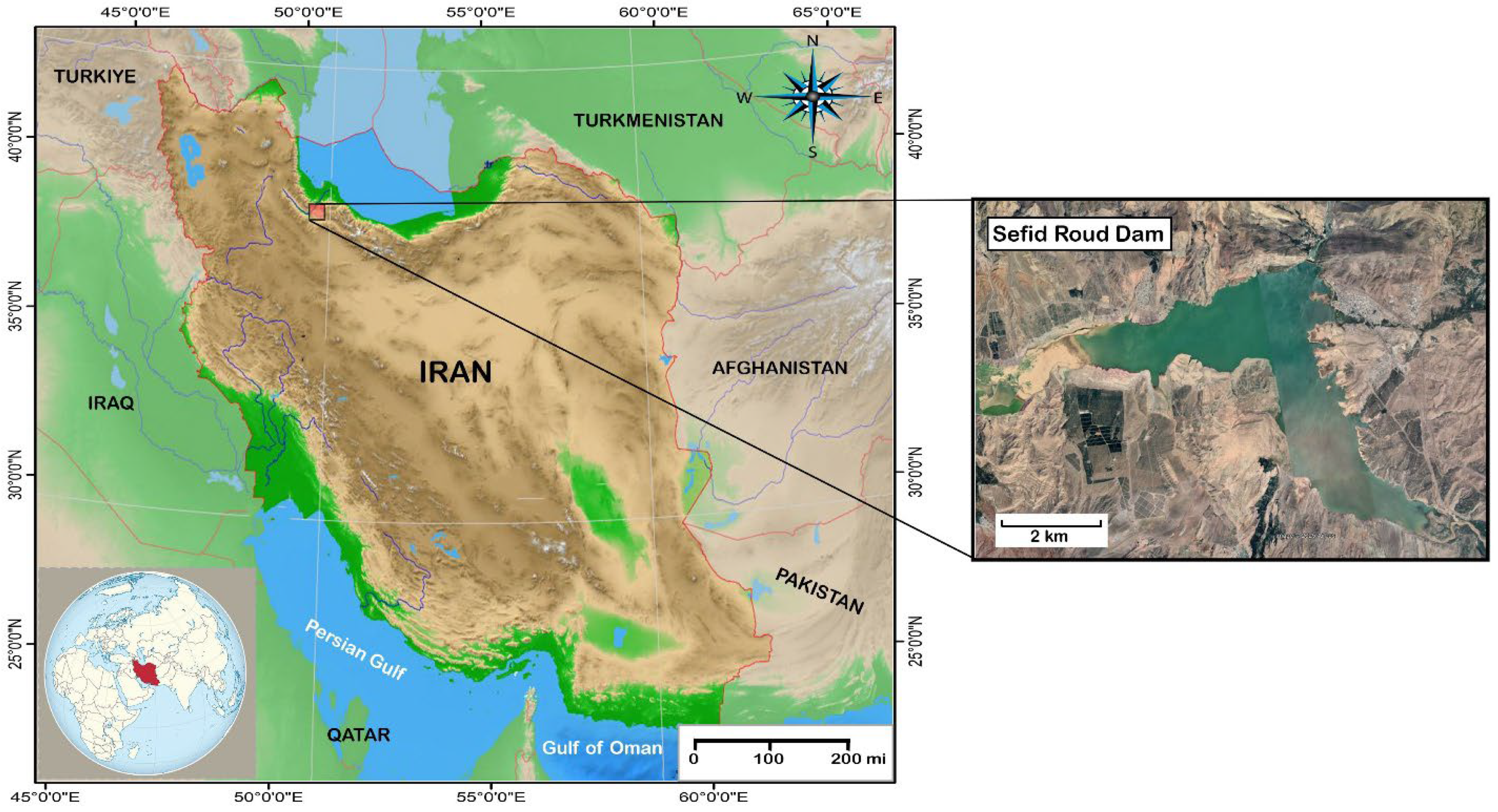
2.1. Overview of the Study Area

In this study, data from the Sefid Roud Dam reservoir in Iran were utilized to forecast the daily inflow and manage the dam’s operation. The Sefid Roud Dam (36°45′31.27″ N, 49°23′16.03″ E), also known as the Manjil Dam, is a significant buttress dam on the Sefid Roud River in Gilan Province, northern Iran [15]. Built in 1962, this dam is crucial for water management, irrigation, and hydroelectric power generation. It has a height of 106 m, a reservoir capacity of approximately 1.82 cubic kilometers, and an installed capacity for hydroelectric power generation of 87.5 megawatts. Figure 1 shows the dam’s location. The Sefid Roud Dam is essential to Gilan’s economy, supporting agricultural productivity and providing a reliable electricity source. This economic importance extends to job creation and improved living standards for local communities. Figure 2 illustrates the time series of the Sefid Roud Dam reservoir inflow over seven years.

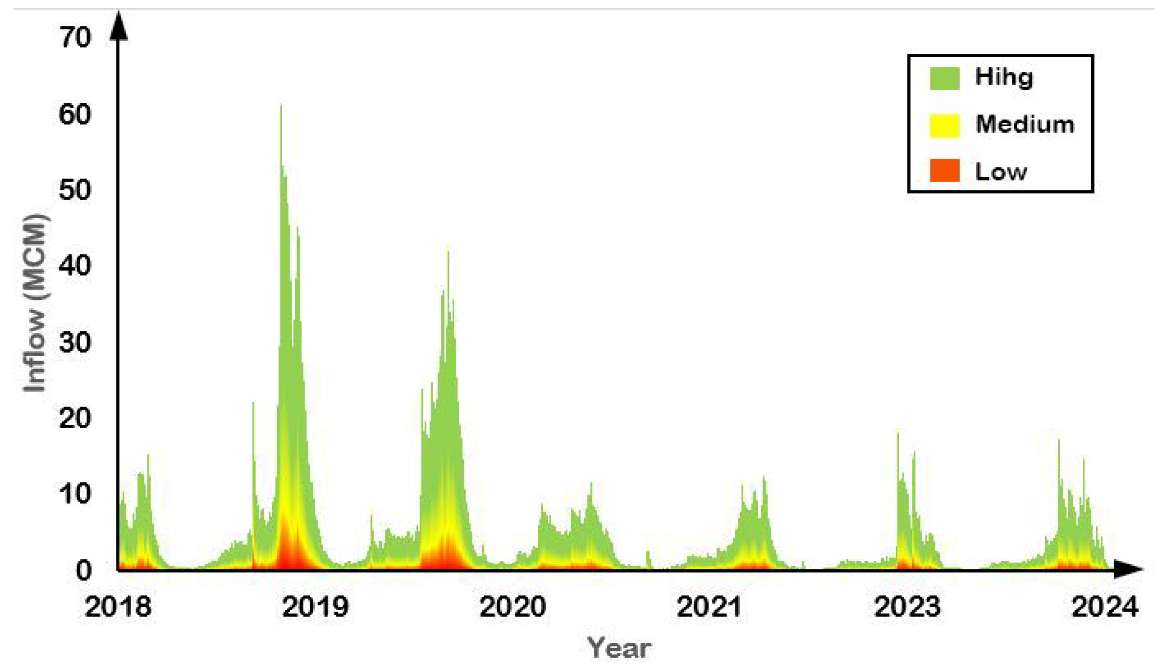
2.2. Overview of the Data Collection and Data Preprocessing

Preprocessing data is essential for preparing raw information for modeling and forecasting. This process involves techniques to improve data quality and suitability for analysis. The main stages of data preprocessing include cleaning, transforming, and reducing data [16]. Proper data preprocessing enhances model accuracy, shortens training time, and improves prediction outcomes. Even advanced models might produce inaccurate results without adequate preprocessing due to poor-quality input data. Therefore, dedicating time to preprocessing is crucial for building effective machine-learning applications.

Some key techniques and stages involved in data preprocessing are data cleaning, data transformation, data reduction, feature engineering, and handling imbalanced data. Data cleaning consists of recognizing and rectifying discrepancies within the dataset, including absent data points, identical entries, and unusual values. Techniques include imputation (filling in missing values), removing duplicates, and handling outliers [17]. The data transformation process entails changing data into an optimal format for analysis. In data analysis, common strategies involve normalization (resizing data to a standard range), standardization (resizing data to establish an average of zero and deviation of one), and encoding categorical variables (transforming categories into numerical values. Data reduction involves minimizing the amount of information without compromising its accuracy. Strategies include reducing dimensionality (lowering the amount of features), choosing key features (selecting the most important ones), and sampling data (picking a portion of the data for examination). Feature engineering involves creating new features from existing data to improve model performance. Techniques include creating interaction terms, aggregating features, and extracting information from date-time variables [18]. To manage imbalanced data sets effectively, one must employ strategies to tackle class disparity, such as oversampling the minority group, under sampling the majority group, or implementing synthetic data generation tools like the Synthetic Minority Over-sampling Technique (SMOTE).

Initially, the desired data were taken from the regional water company. Any data points significantly deviating from other values were either removed or corrected, and missing data were interpolated by the mathematical averaging method to ensure completeness. Subsequently, features were standardized using Z-score normalization to ensure each variable had a mean of zero and a standard deviation of one. About 2% of the data points were corrected due to errors or missing values.

After the data were finalized, two scenarios were used to model and predict daily inflow in terms of million cubic meters (MCM). Scenario One focused on variables such as water level, evaporation rates, and minimum and maximum water temperatures. It is important to note that the daily rainfall in this region is already accounted for within the river inflow data. Scenario Two included delays of inflow data. In wet areas, contrary to dry areas, parameters such as interception or infiltration, as well as the long duration of rainfall, cause the runoff to occur with a delay, and the flood hydrograph becomes wider. Therefore, this research considered a three-day delay as an input. Additionally, using three delays for daily reservoir inflow prediction in wet regions significantly enhances model performance by capturing the short-term memory of the hydrological system. In these areas, frequent and intense rainfall events can lead to runoff and inflow responses that are distributed over several days. Including inflow data from the previous three days allows the model to account for the cumulative effects of recent precipitation, resulting in more accurate and timely predictions, especially during wet spells when inflow can change rapidly. This approach helped us understand how previous inflow patterns impacted the current inflow predictions. The statistical criteria used to evaluate the parameters in these scenarios are listed in

Table 1. Statistical characteristics of the parameters used for the modeling.

Statistical Criteria	Maximum	Average	Minimum	Standard Deviation	Number of Zero
Water Level (m)	272.79	252.01	236.81	10.83	0
Evaporation (MCM)	0.541	0.116	0	0.098	5
Min Temperature (°C)	40.6	12.28	−3	7.86	8
Max Temperature (°C)	45.0	23.91	0	8.22	3
River Inflow (MCM)	41.99	4.026	0.009	5.94	0

. By analyzing these criteria, we gained insights into the factors influencing daily inflow and improved our prediction models.

Univariate modeling refers to statistical techniques used to analyze and model data that involve only one variable or attribute. This approach is commonly applied in both general statistics and time series analysis [19]. Univariate time series models are specifically designed for analyzing sequences of observations recorded over equal intervals. These models predict future values based solely on past values of the same series. Univariate modeling for inflow prediction involves using historical data from a single variable (in this case, past inflow values) to forecast future inflows [20]. This approach is widely used in hydrology and water resources management to predict reservoir or river inflows, which are crucial for managing water supply systems, preventing floods, and optimizing hydropower generation.

Univariate models require only historical data from the variable being forecasted, which can be easier to obtain compared to multivariate models that need additional variables like precipitation or temperature. These models can be quickly developed and deployed, making them useful for situations where rapid forecasting is necessary [21]. Univariate analysis helps identify patterns within the time series, such as trends or seasonality, which are essential for understanding how inflows change over time.

For this study, daily data spanning seven years (2018–2024) were split into training and testing sets. Specifically, 80% of the data (from 18 March 2018 to 19 April 2023) was used for training, while the remaining 20% (from 20 April 2023 to 12 August 2024) was reserved for testing. Modeling was carried out using the following three models: DNN, GRU-LSTM, and bRNN-CNN-GRU within Mathematica software (version 13.3). The hyperparameters employed for these models are detailed in

Table 2. Hyperparameters are used to model DNN, GRU-LSTM, and bRNN-CNN-GRU models.

Type of Parameters	Values/Layer
Network Type	Feed-forward propagation
Data Division	Train (80%) Test (20%)
Number of Hidden Layers (Neurons)	10–55
Batch Size	34–210
learning Function	0.01–0.046
Activation Function	Ramp, Tanh, Cosh
Normalization Function	Batch Normalization
Training Function	Adam

. An overview of the procedures used to predict the reservoir’s inflow is illustrated in Figure 3. Selecting hyperparameters in modeling involves choosing the optimal set of parameters that define a machine learning model’s structure and behavior [22]. Common methods include manual search, which offers fine-grained control but can be time-consuming; grid search, which evaluates all predefined combinations but is computationally intensive; and random search, which efficiently explores the parameter space by randomly sampling combinations. Other approaches, like Hyperband, iteratively narrow down promising regions in the parameter space.

Random search is a hyperparameter optimization technique used to efficiently identify the best set of hyperparameters for machine learning models. Unlike grid search, which exhaustively evaluates all possible combinations from a predefined set, random search samples a fixed number of hyperparameter configurations from specified distributions, evaluating each to find the most effective combination. Random search is often more efficient than grid search, especially when the number of hyperparameters or their possible values is large. Grid search evaluates all combinations, leading to a combinatorial explosion, while random search can explore the space more broadly with fewer evaluations. Therefore, in this study, a random search was used to determine the hyperparameter.

2.3. An Overview of DNN, GRU, and LSTM

A deep neural network is a form of AI that emulates the human mind’s capacity to acquire knowledge and process choices. Deep learning, as opposed to conventional machine learning algorithms that depend on manually crafted features, allows for the automatic learning of features from raw data by utilizing deep neural networks. This allows for more complex and accurate representations of the data, making them ideal for tasks such as image and voice recognition, natural language processing, and autonomous driving [23]. Utilizing deep neural networks in time series data analysis is crucial for accurate forecasting. Deep neural networks can accurately predict future values by analyzing past data points and patterns. This is especially useful in hydrology forecasting, weather prediction, and demand forecasting for businesses.

Each neuron takes in signals from preceding layers, processes them utilizing an activation function, and transmits outputs to the following layers. The output is generally computed as a weighted aggregate of inputs, with an added bias term, filtered through a non-linear activation function. The connection strengths between neurons are governed by parameters called weights.

$$Z={\sum }_{i=1}^n{w}_i{x}_i+b$$

(1)

The weights are denoted as w_i, the inputs as x_i, and the bias term as b.

Neurons are linked by weighted edges, which determine how strongly one neuron influences another [24]. During the learning process, these weights are adjusted to reduce prediction errors. Figure 4 illustrates the structure of the DNN model used in inflow modeling.

Despite their advantages, deep neural networks pose several challenges in time series data analysis. One of the main challenges is the need for a large amount of training data. Deep neural networks require significant amounts of data to effectively learn the underlying patterns, which can be difficult to obtain in certain applications [25]. Furthermore, deep neural networks demand significant computational resources and necessitate high-performance hardware for both training and inference processes. This could impede the progress of smaller organizations or researchers lacking adequate computational resources.

Recent advancements have propelled the gated recurrent unit (GRU) to the forefront of neural network models for analyzing sequential data, notably in time series analysis applications. The GRU design was innovated to overcome the challenge posed by the vanishing gradient problem, a common obstacle faced by recurrent neural networks that affects their capacity to sustain vital long-term associations within sequential data sets. The GRU architecture includes gating mechanisms that control the flow of information within the network, allowing it to selectively update and forget information based on the current input. Enhancing the model’s ability to capture long-range dependencies significantly boosts the performance of time series analysis tasks. It features two primary gates, the reset gate and the update gate. The reset gate controls how much past information is forgotten, while the update gate determines how much new information is added to the hidden state. GRUs compute a candidate activation vector using these gates and then update their hidden state accordingly. With fewer parameters than long short-term memory (LSTM) networks, GRUs are faster to train but often achieve comparable performance in tasks like natural language processing and time-series forecasting [26]. This makes them popular for modeling sequence data when computational efficiency is important.

The update gate decides the proportion of the previous hidden state $\left(h_{t-1}\right)$ that will be included in the current hidden state $\left(h_t\right)$ [27]. It is important to determine whether to retain previous data or update it with fresh information from the latest input $\left(x_t\right)$.

$$Z_t=\sigma (W_t{x}_t+U_z{h}_{t-1}+b_z)$$

(2)

The input and hidden state weight matrices are W_z and U_z, respectively. b_z is the bias term. σ is the sigmoid activation function, which outputs values between 0 and 1 (acting as a gate).

When calculating the candidate hidden state $\left({\tilde{h}}_t\right)$, the reset gate plays a crucial role in deciding how much of the previous hidden state $\left(h_{t-1}\right)$ should be ignored. If the reset gate is close to 0, then it forgets most of the past information.

$$r_t=\sigma (W_r{x}_t+U_r{h}_{t-1}+b_r)$$

(3)

The weight matrices for the input and hidden state are denoted as W_r and U_r, while the bias term is represented as b_r.

The candidate hidden state represents a potential update for the current hidden state $\left(h_t\right)$ [28]. The reset gate (r_t) is utilized in the computation to determine the extent of contribution from the previous hidden state.

$${\tilde{h}}_t=tanh(W_t{x}_t+U_h(r_t\odot h_{t-1})+b_h)$$

(4)

The weight matrix for the input is represented by W_h, while U_h represents the weight matrix for the hidden state [29]. $r_t\odot h_{t-1}$ shows that the reset gate and previous hidden state undergo element-wise multiplication. tanh is the hyperbolic tangent activation function, which outputs values between −1 and 1.

The final hidden state combines the previous hidden state $\left(h_{t-1}\right)$ and the candidate hidden state $\left({\tilde{h}}_t\right)$, controlled by the update gate (z_t). The update gate decides how much of each component contributes to the final hidden state [27], which is shown as follows:

$$h_t=(1-Z_t)\odot h_{t-1}+Z_t\odot {\tilde{h}}_t$$

(5)

where $(1-Z_t)\odot h_{t-1}$ retains part of the previous hidden state, and $Z_t\odot {\tilde{h}}_t$ adds new information from the candidate’s hidden state.

Designed specifically for handling sequential data and capturing long-term relationships, the LSTM model is a distinctive type of recurrent neural network ideal for tasks like time series prediction [30]. They update their hidden states at each time step based on the input from the previous time step and the current feature map. The final output layer processes the information from the LSTM to produce predictions or classifications based on the learned features and temporal dynamics. Unlike standard RNNs, LSTMs use memory cells and gating mechanisms (forget, input, and output gates) to control information flow, preventing the vanishing gradient problem and enabling them to retain information over extended periods [31]. However, LSTMs are computationally intensive and require large datasets for training. Despite their complexity, they remain a powerful tool for sequential data analysis and prediction.

The Selective Memory Gate determines what information is erased from the memory cell. After utilizing the previous concealed state along with the current input, a sigmoid activation function is employed to generate values ranging from 0 (discard) to 1 (keep) for each information fragment. Input gate controls what new information is added to the memory cell [32]. It also uses a sigmoid function to filter incoming data and a tanh function to create a vector of new candidate values that could be added to the cell state. Output gate decides what information from the memory cell is sent to the next layer [33]. It again uses a sigmoid function to filter the cell state before passing it on. The effectiveness of the input gate can be ascertained by employing the following mathematical equation [34]:

$$q_s=\sigma (W_{q[h_s-1,x_s]}+b_s)$$

(6)

$$v_s=tanh(W_{v[h_s-1,x_s]}+b_v)$$

(7)

When considering time s within this process, there are variables, including input gate activation vector q at that moment, which leads to weight matrix W_q impacting previous hidden state h_s−1 and current input x_s alongside bias vector bs, resulting in a new set of values for cell state stored in vs, followed by two additional variables, weight matrix W_v and bias vector b_v. To find the value of forget gate, the following formula is used:

$$p_s=\sigma (W_{p[h_{s-1},x_s]}+b_p)$$

(8)

where hidden state at time s is h_s−1, with Wp symbolizing the weight matrix and x_s as the input; b_p represents the bias vector and p represents the forget gate activation vector. The output gate can be mathematically described by the following equation [34]:

$$f_s=tanh(W_{f[h_s-1,x_s]}+b_f)$$

(9)

$$h_s=f_s\times tanh\left(v_s\right)$$

(10)

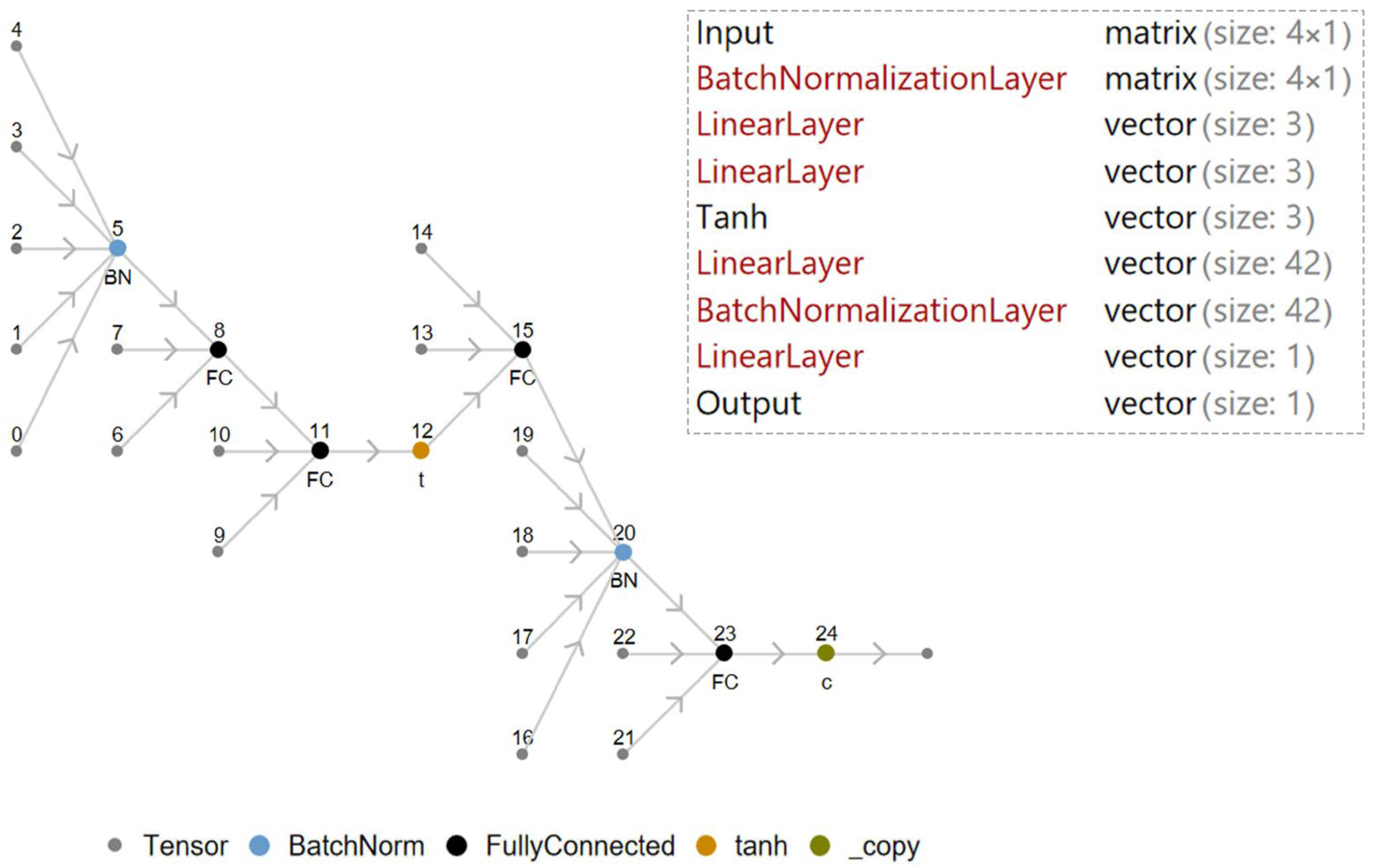
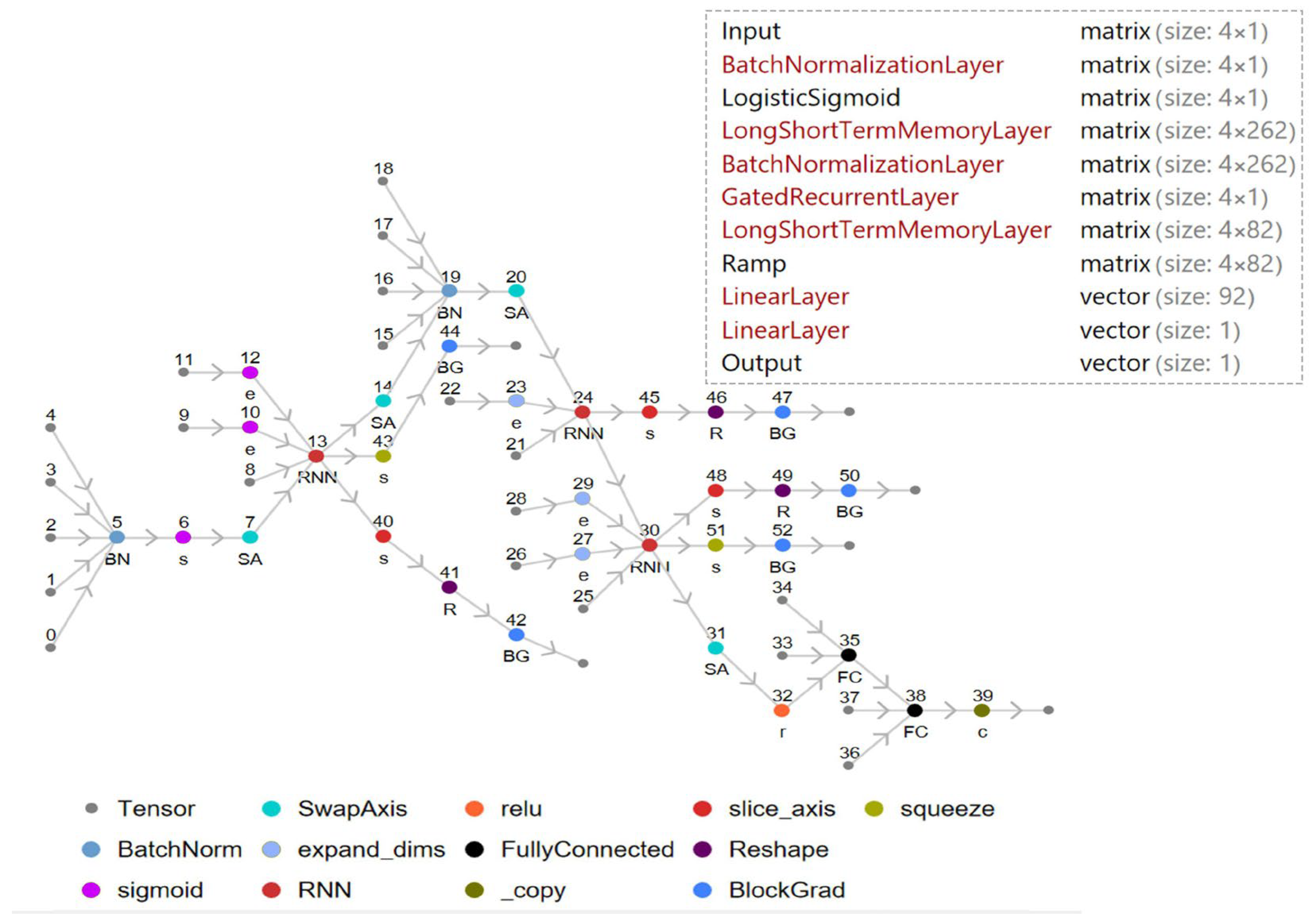
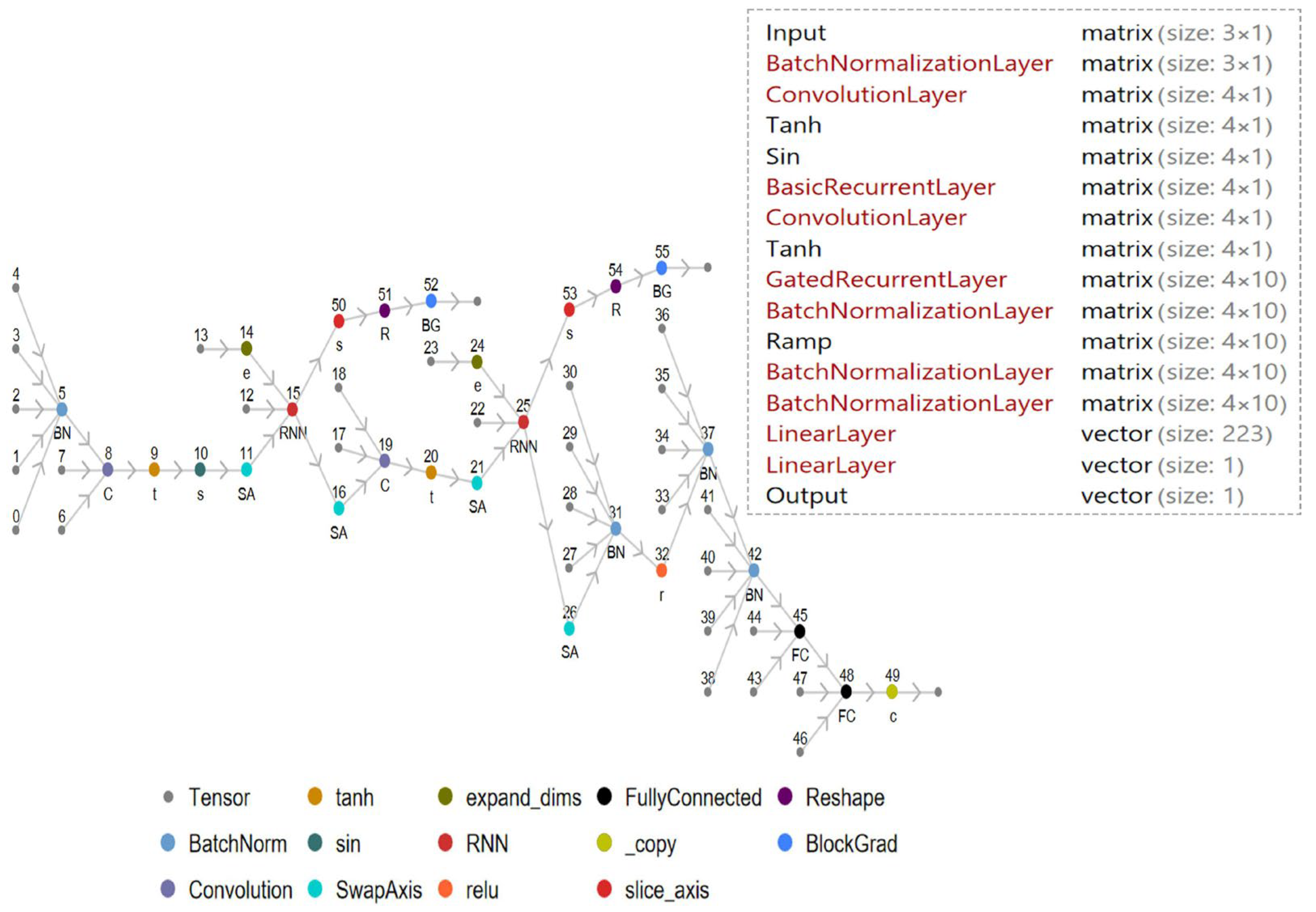
2.4. GRU-LSTM and bRNN-CNN-GRU Hybrid Model

By fusing gated recurrent units (GRUs) with long short-term memory (LSTM) networks, the GRU-LSTM model maximizes the potential of both architectures for handling sequential data tasks. GRUs are simpler and faster, using two gates to manage information flow, while LSTMs are more complex, with three gates, and excel at capturing long-term dependencies. By stacking GRU and LSTM layers, the hybrid model benefits from GRU’s efficiency in feature extraction and LSTM’s robustness in modeling complex temporal relationships. This makes GRU-LSTM models highly effective for tasks like time series forecasting and anomaly detection. However, they require careful tuning and are computationally intensive [35]. Figure 5 shows the structure of the GRU-LSTM model used in the input flow modeling.

A bRNN-CNN-GRU model is a hybrid architecture that combines basic recurrent (bRNN), gated recurrent units (GRUs), and convolutional neural networks (CNNs) to leverage the strengths of third models for sequential and temporal data analysis. This hybrid approach is particularly effective for tasks where the input data have temporal and spatial features, such as time series, and detected data with local patterns [36]. Time series data often contain complex structures, such as trends, seasonality, and noise, which require models capable of capturing short-term and long-term relationships. The bRNN-CNN-GRU model addresses these challenges by leveraging the complementary strengths of CNNs, bRNN, and GRUs. CNNs capture local patterns, while GRUs model long-term dependencies. The hybrid approach often outperforms standalone CNN or GRU models in time series tasks. GRUs are less computationally expensive than LSTMs, making the model faster to train. Additionally, this hybrid model can handle univariate and multivariate time series data. RNNs can struggle with long-term dependencies due to the vanishing gradient problem. The novelty of combining bRNN, CNN, and GRU models is in their synergistic integration—CNNs extract meaningful local features, GRUs capture temporal dynamics efficiently, and bRNNs provide bidirectional context—resulting in models that outperform individual architectures in accuracy, robustness, and applicability across diverse sequential and spatial data tasks.

The bRNN-CNN-GRU model, which combines basic recurrent, gated recurrent units, and convolutional neural networks, is powerful for time series analysis but faces several challenges. These include design and hyperparameter tuning complexity, high computational costs, and the risk of overfitting, especially with small or noisy datasets. Preprocessing time series data (e.g., normalization, handling missing values) and choosing the right sequence length are critical but challenging. Additionally, bRNN-CNN-GRUs are difficult to interpret, making them less suitable for domains requiring explainability. Handling multivariate time series, noisy or irregular data, and scaling to large datasets further complicate their use. Despite these challenges, strategies like regularization, data augmentation, and efficient architectures can mitigate these issues, making bRNN-CNN-GRUs a robust choice for time series tasks when implemented carefully. Figure 6 shows the structure of the bRNN-CNN-GRU model used in the inflow modeling.

2.5. Model Training Scenarios

In this study, univariate and multivariate scenarios are chosen because they represent the following fundamentally different but complementary approaches: univariate for focused, simple analysis of single outcomes, and multivariate for integrated, comprehensive analysis of multiple outcomes simultaneously. This choice allows researchers to control error rates, understand complex relationships, improve predictions, and communicate findings effectively.

Multivariate modeling, which incorporates variables like water level, evaporation, Tmin, and Tmax, offers the advantage of capturing complex relationships and interactions among multiple factors. This approach better reflects real-world environmental dynamics and often leads to more accurate and robust predictions by considering how these variables influence each other simultaneously. However, the increased complexity requires more computational resources, careful data handling, and expertise to avoid issues such as overfitting and sensitivity to noisy or incomplete data.

In contrast, univariate modeling focuses on analyzing one variable at a time, such as First Delay, Second Delay, and Third Delay in this study. This simplicity makes univariate models easier to implement, interpret, and compute, which is beneficial for quick analyses or when the primary interest lies in understanding individual variables. Nonetheless, univariate models do not account for interactions between variables, which can limit their predictive power and oversimplify systems where multiple factors jointly affect outcomes.

Table 3. Division of the evaluated scenarios to predict the input flow of the tank with two models: DNN, GRU-LSTM, and bRNN-CNN-GRU.

Scenario	Input	Model	Output
Scenario (1)	Water Level, Evaporation, Tmin, Tmax	DNN, GRU-LSTM, bRNN-CNN-GRU	Reservoir Inflow
Scenario (2)	First Delay, Second Delay, Third Delay	DNN, CNN-LSTM, bRNN-CNN-GRU	Reservoir Inflow

presents the scenarios assessed in this study. The first scenario incorporates hydrological parameters and reservoir water parameters (multivariate). The second scenario examines the delays in reservoir inflow (univariate).

2.6. Model Evaluation Metrics

Evaluating models is a key component of machine learning, as it examines the performance and quality of trained models. This evaluation is essential for various reasons, all of which enhance the efficiency and dependability of machine learning applications. Root mean square error (RMSE) is a popular metric used to gauge the accuracy of predictions generated by machine learning models [37]. It measures the average discrepancy between predicted and actual values, offering insights into the model’s performance. The minimum possible value for RMSE is 0, signifying an ideal fit where predicted, and the actual values align perfectly. In this case, all residuals (differences between predicted and actual values) are zero. RMSE has no theoretical maximum and can extend to positive infinity. The RMSE value rises as the discrepancies between predicted and actual values increase, particularly if there are significant outliers in the dataset [38].

Pearson’s correlation is a statistical metric that measures the degree to which two or more variables move in relation to each other. It shows how changes in one variable are linked to changes in another without suggesting causation. Positive correlation occurs when two variables move in the same direction; as one variable increases, the other does as well, and vice versa [39]. A negative correlation happens when one variable rises while the other falls. Zero correlation indicates no relationship between the two variables, meaning changes in one do not predict changes in the other. Additionally, in this research, this method was used to find the relationship between the model input and the output, which is the water level. Understanding the connection between model input and output through Pearson’s correlation coefficient is crucial, as it measures how strongly and in what direction input variables are linearly associated with the output. This enables researchers to discern influential factors, refine models effectively, and interpret their behavior with greater clarity.

The Nash–Sutcliffe efficiency (NSE) is a common metric in hydrological modeling used to evaluate model performance by comparing simulated data to observed data [40]. When the NSE value equals 1, it indicates a flawless correlation between the forecasted results and the actual observations; conversely, an NSE of 0 reveals that the model’s accuracy is no better than if one were to utilize the mean of the observed data. The presence of negative NSE values indicates that using the mean of the available data produces superior forecasts compared to the model itself. Together, these metrics provide a balanced evaluation; RMSE reports absolute error magnitude, NSE assesses relative predictive skill, and correlation captures pattern agreement. This combination ensures a comprehensive understanding of model accuracy, reliability, and usefulness in time series modeling.

$$RMSE=\sqrt{{{\displaystyle \frac{1}{N}}{\sum }_{i=1}^N(X_{pi}-X_{oi})}^2}$$

(11)

$$r={\displaystyle \frac{{\sum }_{i=1}^N\left(X_{oi}-\overline{X_o}\right)\left(X_{pi}-\overline{X_p}\right)}{\sqrt{{\sum }_{i=1}^N{\left(X_{oi}-\overline{X_o}\right)}^2 . {\sum }_{i=1}^N{\left(X_{pi}-\overline{X_p}\right)}^2 }}}$$

(12)

$$NSE=1-\left[{\displaystyle \frac{{\sum }_{i=1}^n{(X_{pi}-X_{oi})}^2}{{\sum }_{i=1}^n{(X_{pi}-\overline{X_p})}^2}}\right]$$

(13)

3. Experimental Results and Discussion

Including parameters with weak correlation to the target variable in machine learning models can still be valuable because correlation only captures linear relationships. These features may have nonlinear or interaction effects that contribute important predictive information, especially when using advanced algorithms capable of modeling complex patterns. Additionally, weakly correlated parameters might provide complementary insights that improve the model’s generalization and help capture indirect or delayed influences, such as how precipitation and temperature affect reservoir inflow over time. Overall, while a strong correlation is a useful guideline, including parameters with a weak correlation can enhance model performance when handled carefully and supported by domain knowledge. Figure 7 illustrates the correlations between the desired parameters. Based on these correlations, it is evident that the water level in the first scenario and all three delays in the second scenario exhibit a strong correlation with the reservoir’s input.

Table 4. Evaluation criteria for three, DNN, GRU-LSTM, and bRNN-CNN-GRU, models.

Scenario	Model	r	RMSE (MCM)	NSE
Scenario (1)	DNN	0.7803	2.0176	0.5785
	GRU-LSTM	0.8276	1.9853	0.5984
	bRNN-CNN-GRU	0.8706	1.7217	0.7323
Scenario (2)	DNN	0.9485	1.3354	0.8132
	GRU-LSTM	0.9677	0.8584	0.9233
	bRNN-CNN-GRU	0.9734	0.7099	0.9474

details the evaluation metrics for the three models, DNN, GRU-LSTM, and bRNN-CNN-GRU. In the first scenario, the DNN model performed poorly, with an error of 2.017, r of 0.780, and NSE of 0.578. In the second scenario, its performance improved, showing an error of 1.335, r of 0.948, and NSE of 0.813. In the first scenario, the GRU-LSTM model recorded an error of 1.985, r of 0.827, and NSE of 0.598. In the second scenario, it performed well with an error of 0.858, r of 0.967, and NSE of 0.923, surpassing the DNN model in both cases. In scenario one, the bRNN-CNN-GRU model achieved a 1.721 error, 0.870 r value, and 0.732 NSE. In the second scenario, it performed with an error of 0.709, r of 0.973, and NSE of 0.947.

According to the obtained results, DNN, GRU-LSTM, and bRNN-CNN-GRU models performed better in the second scenario. Hence, while univariate modeling has its place in certain contexts due to its simplicity and efficiency, it is generally not considered superior overall when compared to multivariable approaches that provide more comprehensive insights into data relationships. Additionally, according to the results obtained for the first scenario, this scenario has its own importance. Daily inflow measurement is difficult and expensive, especially in large dams. On the other hand, the measurement of parameters related to water and hydrology, which, in this research, includes water level, evaporation, and maximum and minimum temperature, is easier and less complicated in terms of application.

Table 5. Statistical characteristics of the parameters used for the actual and three experimental models.

Scenario	Model	Maximum	Average	Minimum	Standard Deviation
	Actual	17.194	2.762	0.043	3.095
Scenario (1)	DNN	8.343	3.203	0.183	2.302
	GRU-LSTM	13.376	2.497	0.026	2.766
	bRNN-CNN-GRU	16.391	2.631	0.450	2.512
Scenario (2)	DNN	15.508	3.629	1.772	2.758
	GRU-LSTM	14.517	2.757	0.770	2.620
	bRNN-CNN-GRU	16.186	2.795	0.195	2.971

shows the statistical characteristics for the observed values and the three models, DNN, GRU-LSTM, and bRNN-CNN-GRU. According to the statistical characteristics of the hybrid bRNN-CNN-GRU model, which has a maximum (16.39), an average (2.63), a minimum (0.45), and a standard deviation (2.51) in the first scenario and a maximum (16.18), an average (2.79), a minimum (0.19), and a standard deviation (2.97) in the second scenario, compared to the actual values with a maximum (17.19), an average (2.76), and a minimum (0.043) and standard deviation (3.09), it has high performance and reliability compared to other models.

Three types of graphical plots—time series, scatter, and box—were employed to assess the three models’ performance in predicting and modeling daily inflow. According to Figure 8, which shows the time series graph for two scenarios, the DNN model in the first scenario shows a higher fit than the actual values in most places and has a large error in the maximum and minimum points. In the second scenario, this model has significant errors compared to the real values, but it is slightly improved compared to the first scenario. In the first and second scenarios, the GRU-LSTM model has lower predictions than the actual values in some places and has a disproportion, but this error is less than the DNN model. Conversely, the combined bRNN-CNN-GRU model demonstrated strong performance across both scenarios. Additionally, predicted values showed minimal deviations from the actual values.

Figure 9 illustrates the scatter diagrams of three models across two scenarios with varying inputs. The DNN model exhibited different dispersion patterns in each scenario. In the first scenario, it achieved a coefficient of 0.78, which increased to 0.94 in the second scenario. Additionally, the GRU-LSTM model showed a coefficient of 0.82 in the first scenario and 0.96 in the second scenario. The bRNN-CNN-GRU model exhibited less dispersion in the second scenario than the first, with a coefficient of 0.87 in the first scenario and 0.97 in the second. Based on the dispersion and coefficients of the models in both scenarios, it is evident that all three models performed better in the second scenario than in the first. Additionally, the bRNN-CNN-GRU model displayed less dispersion compared to the DNN and GRU-LSTM models.

Figure 10 shows the box plot of the three models, DNN, GRU-LSTM, and bRNN-CNN-GRU, for two scenarios. In the first scenario, the DNN model’s resemblance to the real values was lacking based on this diagram, but conversely, in the second scenario, the model demonstrated enhanced performance and approaches closer to the actual values. The GRU-LSTM model also performed poorly in the first scenario, but the performance of the model increased in the second scenario. On the other hand, the bRNN-CNN-GRU model, with optimal performance in both scenarios compared to the DNN and GRU-LSTM models, was very similar to the real values and had high reliability.

A lower error in univariate modeling compared to multivariate modeling does not necessarily indicate the high performance of univariate modeling. Univariate models are simpler and focus on a single variable or relationship, which can result in lower errors if the data are well-behaved and primarily driven by that single factor [41]. However, this simplicity might overlook important interactions between variables that multivariate models capture. Multivariate models account for multiple variables simultaneously, reducing omitted variable bias (a situation where leaving out relevant variables can distort estimates). If a multivariate model shows higher error due to omitted variable bias being mitigated, it does not mean it performs worse; rather, it provides a more comprehensive view of relationships.

The evaluated criteria and graphical charts indicate that the bRNN-CNN-GRU model demonstrated high accuracy in predicting dam reservoir inflow. Additionally, based on the results, all three models performed better in the second scenario, which includes input parameters with three delays in the input flow, compared to the first scenario.

The bRNN-CNN-GRU hybrid model merges the advantages of three unique neural network structures—bRNN, GRU, and CNN—to improve daily reservoir inflow predictions. This combination is particularly effective for managing the complexities of hydrological data, which often display non-linear trends and temporal relationships. CNNs are adept at extracting spatial features from data, which is beneficial for analyzing high-dimensional or spatially distributed time series data [42]. This capability helps filter noise and extract meaningful patterns that might not be evident through temporal analysis alone. By integrating CNNs with GRUs, these models can leverage both spatial pattern recognition and efficient temporal modeling capabilities. This hybrid approach enhances prediction accuracy by considering multiple aspects of the data simultaneously.

Moreover, the bRNN-CNN-GRU architecture benefits from improved generalization and training stability. Techniques like dropout and input windowing reduce overfitting, resulting in more reliable outcomes across different datasets and scenarios. Compared to standalone DNNs or GRU-LSTM hybrids, this model better balances complexity and efficiency, capturing a wider range of data patterns while maintaining faster training times. These combined advantages make the bRNN-CNN-GRU model particularly effective for complex forecasting and prediction tasks involving sequential and spatial data. This synergy enables it to better capture the complex, nonlinear, and seasonal dynamics of inflow time series while maintaining computational efficiency, leading to more accurate and reliable forecasts for reservoir management.

Recent studies have increasingly focused on hybrid models that combine various deep-learning architectures to improve the prediction of reservoir inflows and related hydrological processes. Hadiyan et al. [43] explored the use of varying models of artificial neural networks (ANN), both static and dynamic, such as static feed-forward neural network (FFNN), non-linear autoregressive (NAR), and nonlinear autoregressive with exogenous inputs (NARX) for predicting Sefid Roud Dam reservoir inflows. The findings indicated that the NAR model had superior performance, with an average error of 588 cubic meters per second and a coefficient of determination of 0.85, outshining all other models. Li et al. [44] investigated water-level forecasting for the Three Gorges Reservoir using a CNN-Attention-LSTM model. Their approach greatly improved prediction accuracy, especially for extreme cases, achieving an R² value of 0.994. In their 2023 study, Yao et al. [45] presented a cutting-edge design incorporating CNN-LSTM and GRU models with dynamic weighting bolstered by the innovative Sparrow Search Algorithm (ISSA). This model offers a reliable approach to predicting river runoff by leveraging historical meteorological and runoff data. The model, tested across different watersheds, achieved remarkable performance, with a Nash–Sutcliffe efficiency (NSE) value of 0.90 in the Bailong River watershed, underscoring its potential in effective water resource management and flood mitigation. Gou et al. [13] put forth an upgraded hydrological model by merging ensemble learning and residual error correction methods. The accuracy increased by employing three deep learning models (ED-GRU, ED-LSTM, and CNN-LSTM) and merging their outputs into a categorical gradient boosting regression (CGBR) model. The proposed hybrid model significantly improved the prediction of hourly inflow in reservoirs, achieving an average performance improvement of 66.2% compared to standalone DL models. It effectively predicts peak and total inflows during storm events with multi-peak hydrographs. Zamani et al. [46] employed two distinctive deep learning algorithms, convolutional neural networks (CNNs), and gated recurrent units (GRUs). They also combined these methods to create a CNN-GRU model, which effectively measured the concentration of various indicators in a reservoir. Additionally, they developed two separate machine learning (ML) algorithms, random forest (RF) and support vector regression (SVR). This was done to showcase the superior performance of deep learning algorithms compared to individual ML ones. The CNN-GRU model proved superior to all other algorithms by showing a 13% increase over SVR and RF, a 9% increase over CNN, and an 8% increase over GRU when assessed with R-squared and DO as performance indicators alongside WQIs. Khorram and Jehbez [47] evaluated hybrid models (SVM-GA, ANFIS-GA, ARIMA-LSTM) against standalone models (LSTM, SVM, ANFIS, ARIMA) and the SWAT hydrological model for forecasting inflows into Iran’s Droodzan Dam reservoir. Using statistical metrics (RMSE, MAE, MAPE, MSE, R²), results demonstrated that hybrid models outperformed individual ones, with ARIMA-LSTM achieving the highest accuracy (R² = 0.9272 training, 0.9097 testing). The findings highlight ARIMA-LSTM’s superior reliability for monthly inflow prediction in arid/semi-arid regions, offering a robust tool for water resource planning. Shabbir et al. [48] proposed a novel hybrid model, HF-LMD-EEMD-KNN (HLEK), for daily river inflow prediction, integrating outlier correction (Hampel filter), dual-stage signal decomposition (Local Mean Decomposition + Ensemble Empirical Mode Decomposition), and K-nearest neighbor (KNN) forecasting. Evaluated on four Indus River Basin datasets, HLEK outperformed conventional models, achieving training-phase MAEs of 7.072 (Indus), 5.859 (Kabul), 2.308 (Jhelum), and 3.709 (Chenab).

The bRNN-CNN-GRU model’s superior accuracy in forecasting reservoir inflow directly enhances reservoir management by enabling more precise predictions of water availability. This allows operators to optimize reservoir releases and storage, balancing critical needs such as flood control, irrigation, hydropower generation, and ecological conservation. Improved forecast reliability reduces uncertainty, supporting confident and informed decision-making under variable hydrological conditions.

Additionally, the model’s efficient architecture, combining CNN’s feature extraction with GRU’s streamlined sequence learning, ensures high performance without excessive computational demands. This makes it practical for real-time monitoring and adaptive reservoir operation, where timely responses to changing inflow patterns are essential. The model’s ability to capture complex, nonlinear, and seasonal inflow dynamics further supports sustainable water resource utilization and risk management.

4. Conclusions

By combining historical data with machine learning models, this study created a system for the daily assessment and prediction of reservoir inflow to improve water resource management. Using data from the Sefid Roud Dam reservoir, two scenarios were created, incorporating water parameters and three delays of inflow data. Results indicated that the DNN, GRU-LSTM, and bRNN-CNN-GRU models in the second scenario performed better than those in other scenarios.

The use of bRNN-CNN-GRU models for dam inflow prediction faces several limitations. These models require large amounts of high-quality data to perform well, and their complexity can lead to overfitting if not appropriately managed. They often struggle with predicting high flow rates during extreme weather events and may not handle seasonal fluctuations effectively unless specifically designed to do so. Additionally, predictive performance tends to decrease as the lead time increases, making long-term forecasts less reliable. Furthermore, these models typically do not account for uncertainties inherent in hydrological observations, which could be improved by incorporating uncertainty quantification methods. While bRNN-CNN-GRU combinations show promise in certain contexts, they may not consistently outperform other advanced techniques across all scenarios. Although we can increase the accuracy of the model by increasing the number of delays in the input and increasing the number of hidden layers, this work causes excessive complexity and makes it difficult to understand. This is why the precision obtained in this research is desirable and reasonable for the conditions of Iran.

Future research in dam inflow prediction using bRNN-CNN-GRU models should focus on several key areas. This includes developing hybrid models that combine bRNN-CNN-GRUs with other techniques to enhance accuracy and robustness, particularly during extreme events. Additionally, incorporating uncertainty quantification methods will improve model reliability under varying conditions. Real-time prediction systems should be developed for operational integration into dam management frameworks. Furthermore, integrating climate change impacts and combining deep learning with physically based hydrological models will provide a more comprehensive understanding of water flow dynamics over long-term horizons. Future research should explore integrating additional data sources, such as precipitation forecasts, soil moisture, remote sensing data, and catchment characteristics, to improve model robustness and forecasting accuracy. Additionally, this reservoir is modeled for a humid region in Iran; thus, it can be modeled for dry regions in the future. Hence, effective use in dry regions demands adaptation through retraining, transfer learning, or integration with physical hydrological models to capture the distinct hydrological processes of dry climates.

References

1. Khedre, A.M.; Ramadan, S.A.; Ashry, A.; Alaraby, M. Abundance and Risk Assessment of Microplastics in Water, Sediment, and Aquatic Insects of the Nile River. Chemosphere 2024, 353, 141557. [Google Scholar] [CrossRef] [PubMed]
2. Połomski, M.; Wiatkowski, M. Impounding Reservoirs, Benefits and Risks: A Review of Environmental and Technical Aspects of Construction and Operation. Sustainability 2023, 15, 16020. [Google Scholar] [CrossRef]
3. García-Feal, O.; González-Cao, J.; Fernández-Nóvoa, D.; Astray Dopazo, G.; Gómez-Gesteira, M. Comparison of machine learning techniques for reservoir outflow forecasting. Nat. Hazards Earth Syst. Sci. Discuss. 2022, 2022, 1–27. [Google Scholar] [CrossRef]
4. Babaei, M.; Moeini, R.; Ehsanzadeh, E. Artificial Neural Network and Support Vector Machine Models for Inflow Prediction of Dam Reservoir (case study: Zayandehroud Dam Reservoir). Water Resour. Manag. 2019, 33, 2203–2218. [Google Scholar] [CrossRef]
5. Emadi, A.; Zamanzad-Ghavidel, S.; Boroomandnia, A.; Fazeli, S.; Sobhani, R. Modeling the Total Outflow of Reservoirs Using Wavelet-Developed Approaches: A Case Study of the Mahabad Dam Reservoir, Iran. Water Supply 2023, 23, 4645–4671. [Google Scholar] [CrossRef]
6. Chang, Z.; Jiang, Z.; Wang, P. Inflow combination forecast of reservoir based on SWAT, XAJ model and Bayes model averaging method. Water Supply 2022, 22, 8440–8464. [Google Scholar] [CrossRef]
7. Rahman, K.U.; Balkhair, K.S.; Almazroui, M.; Masood, A. Sub-Catchments Flow Losses Computation Using Muskingum–Cunge Routing Method and HEC-HMS GIS Based Techniques, Case Study of Wadi Al-Lith, Saudi Arabia. Model. Earth Syst. Environ. 2017, 3, 4. [Google Scholar] [CrossRef]
8. Salvati, A.; Moghaddam Nia, A.; Salajegheh, A.; Shirzadi, A.; Shahabi, H.; Ahmadisharaf, E.; Clague, J.J. A Systematic Review of Muskingum Flood Routing Techniques. Hydrol. Sci. J. 2024, 69, 810–831. [Google Scholar] [CrossRef]
9. Myronidis, D.; Ioannou, K.; Fotakis, D.; Dörflinger, G. Streamflow and Hydrological Drought Trend Analysis and Forecasting in Cyprus. Water Resour. Manag. 2018, 32, 1759–1776. [Google Scholar] [CrossRef]
10. Nguyen, X.H. Combining Statistical Machine Learning Models with ARIMA for Water Level Forecasting: The Case of the Red River. Adv. Water Resour. 2020, 142, 103656. [Google Scholar]
11. Wegayehu, E.B.; Muluneh, F.B. Multivariate streamflow simulation using hybrid deep learning models. Comput. Intell. Neurosci. 2021, 2021, 5172658. [Google Scholar] [CrossRef] [PubMed]
12. Zhou, F.; Chen, Y.; Liu, J. Application of a new hybrid deep learning model that considers temporal and feature dependencies in rainfall–runoff simulation. Remote Sens. 2023, 15, 1395. [Google Scholar] [CrossRef]
13. Guo, W.D.; Chen, W.B.; Chang, C.H. Prediction of hourly inflow for reservoirs at mountain catchments using residual error data and multiple-ahead correction technique. Hydrol. Res. 2023, 54, 1072–1093. [Google Scholar] [CrossRef]
14. Moeini, R.; Nasiri, K.; Hosseini, S.H. Predicting the Water Inflow into the Dam Reservoir Using the Hybrid Intelligent GP-ANN-NSGA-II Method. Water Resour. Manag. 2024, 38, 4137–4159. [Google Scholar] [CrossRef]
15. Neshaei, S.A.; Mehrdad, M.A.; Molatefat, S.H. Investigation of discharge and sedimentation rates of the sefid-roud river after de-siltation of the sefid-roud dam, Iran. WIT Trans. Ecol. Environ. 2017, 221, 1–12. [Google Scholar]
16. García, S.; Luengo, J.; Herrera, F. Data Preprocessing in Data Mining; Springer International Publishing: Cham, Switzerland, 2015; Volume 72, pp. 59–139. [Google Scholar]
17. Wang, S.; Celebi, M.E.; Zhang, Y.D.; Yu, X.; Lu, S.; Yao, X.; Tyukin, I. Advances in data preprocessing for biomedical data fusion: An overview of the methods, challenges, and prospects. Inf. Fusion 2021, 76, 376–421. [Google Scholar] [CrossRef]
18. Peng, S.; Sun, S.; Yao, Y.D. A survey of modulation classification using deep learning: Signal representation and data preprocessing. IEEE Trans. Neural Netw. Learn. Syst. 2021, 33, 7020–7038. [Google Scholar] [CrossRef]
19. Lee, S.; Kim, J.; Bae, J.H.; Lee, G.; Yang, D.; Hong, J.; Lim, K.J. Development of multi-inflow prediction ensemble model based on auto-sklearn using combined approach: Case study of soyang river dam. Hydrology 2023, 10, 90. [Google Scholar] [CrossRef]
20. Petropoulos, F.; Svetunkov, I. A simple combination of univariate models. Int. J. Forecast. 2020, 36, 110–115. [Google Scholar] [CrossRef]
21. Abdel-Aal, R.E. Univariate modeling and forecasting of monthly energy demand time series using abductive and neural networks. Comput. Ind. Eng. 2008, 54, 903–917. [Google Scholar] [CrossRef]
22. Yang, L.; Shami, A. On hyperparameter optimization of machine learning algorithms: Theory and practice. Neurocomputing 2020, 415, 295–316. [Google Scholar] [CrossRef]
23. Agatonovic-Kustrin, S.; Beresford, R. Basic concepts of artificial neural network (ANN) modeling and its application in pharmaceutical research. J. Pharm. Biomed. Anal. 2000, 22, 717–727. [Google Scholar] [CrossRef] [PubMed]
24. Mai, H.V.T.; Nguyen, T.A.; Ly, H.B.; Tran, V.Q. Investigation of ANN Model Containing One Hidden Layer for Predicting Compressive Strength of Concrete with Blast-Furnace Slag and Fly Ash. Adv. Mater. Sci. Eng. 2021, 2021, 5540853. [Google Scholar] [CrossRef]
25. Mittal, S. A Survey on Modeling and Improving Reliability of DNN Algorithms and Accelerators. J. Syst. Archit. 2020, 104, 101689. [Google Scholar] [CrossRef]
26. Zhen, L.; Bărbulescu, A. Comparative Analysis of Convolutional Neural Network-Long Short-Term Memory, Sparrow Search Algorithm-Backpropagation Neural Network, and Particle Swarm Optimization-Extreme Learning Machine Models for the Water Discharge of the Buzău River, Romania. Water 2024, 16, 289. [Google Scholar] [CrossRef]
27. Xu, S.; Li, J.; Liu, K.; Wu, L. A parallel GRU recurrent network model and its application to multi-channel time-varying signal classification. IEEE Access 2019, 7, 118739–118748. [Google Scholar] [CrossRef]
28. Choe, D.E.; Kim, H.C.; Kim, M.H. Sequence-Based Modeling of Deep Learning with LSTM and GRU Networks for Structural Damage Detection of Floating Offshore Wind Turbine Blades. Renew. Energy 2021, 174, 218–235. [Google Scholar] [CrossRef]
29. Ge, K.; Zhao, J.Q.; Zhao, Y.Y. Gr-gnn: Gated recursion-based graph neural network algorithm. Mathematics 2022, 10, 1171. [Google Scholar] [CrossRef]
30. Madaeni, F.; Chokmani, K.; Lhissou, R.; Gauthier, Y.; Tolszczuk-Leclerc, S. Convolutional neural network and long short-term memory models for ice-jam predictions. Cryosphere 2022, 16, 1447–1468. [Google Scholar] [CrossRef]
31. Sunny, M.A.I.; Maswood, M.M.S.; Alharbi, A.G. Deep learning-based stock price prediction using LSTM and bi-directional LSTM model. In Proceedings of the 2020 2nd Novel Intelligent and Leading Emerging Sciences Conference (NILES), Giza, Egypt, 24–26 October 2020; pp. 87–92. [Google Scholar]
32. Le, X.H.; Ho, H.V.; Lee, G.; Jung, S. Application of long short-term memory (LSTM) neural network for flood forecasting. Water 2019, 11, 1387. [Google Scholar] [CrossRef]
33. Nifa, K.; Boudhar, A.; Ouatiki, H.; Elyoussfi, H.; Bargam, B.; Chehbouni, A. Deep Learning Approach with LSTM for Daily Streamflow Prediction in a Semi-Arid Area: A Case Study of Oum Er-Rbia River Basin, Morocco. Water 2023, 15, 262. [Google Scholar] [CrossRef]
34. Yu, Y.; Si, X.; Hu, C.; Zhang, J. A review of recurrent neural networks: LSTM cells and network architectures. Neural Comput. 2019, 31, 1235–1270. [Google Scholar] [CrossRef] [PubMed]
35. Cao, B.; Li, C.; Song, Y.; Qin, Y.; Chen, C. Network Intrusion Detection Model Based on CNN and GRU. Appl. Sci. 2022, 12, 4184. [Google Scholar] [CrossRef]
36. Jafari, S.; Byun, Y.C. A CNN-GRU Approach to the Accurate Prediction of Batteries’ Remaining Useful Life from Charging Profiles. Computers 2023, 12, 219. [Google Scholar] [CrossRef]
37. Chai, T.; Draxler, R.R. Root Mean Square Error (RMSE) or Mean Absolute Error (MAE). Geosci. Model Dev. Discuss. 2014, 7, 1525–1534. [Google Scholar]
38. Ćalasan, M.; Aleem, S.H.A.; Zobaa, A.F. On the Root Mean Square Error (RMSE) Calculation for Parameter Estimation of Photovoltaic Models: A Novel Exact Analytical Solution Based on Lambert W Function. Energy Convers. Manag. 2020, 210, 112716. [Google Scholar] [CrossRef]
39. Asuero, A.G.; Sayago, A.; González, A.G. The correlation coefficient: An overview. Crit. Rev. Anal. Chem. 2006, 36, 41–59. [Google Scholar] [CrossRef]
40. Duc, L.; Sawada, Y. A Signal-Processing-Based Interpretation of the Nash–Sutcliffe Efficiency. Hydrol. Earth Syst. Sci. 2023, 27, 1827–1839. [Google Scholar] [CrossRef]
41. Santos, A.A.; Nogales, F.J.; Ruiz, E. Comparing univariate and multivariate models to forecast portfolio value-at-risk. J. Financ. Econom. 2013, 11, 400–441. [Google Scholar] [CrossRef]
42. Moodi, F.; Jahangard Rafsanjani, A.; Zarifzadeh, S.; Zare Chahooki, M.A. Advanced Stock Price Forecasting Using a 1D-CNN-GRU-LSTM Model. J. AI Data Min. 2024, 12, 393–408. [Google Scholar]
43. Hadiyan, P.P.; Moeini, R.; Ehsanzadeh, E. Application of Static and Dynamic Artificial Neural Networks for Forecasting Inflow Discharges, Case Study: Sefidroud Dam Reservoir. Sustain. Comput. Inform. Syst. 2020, 27, 100401. [Google Scholar] [CrossRef]
44. Li, H.; Zhang, L.; Zhang, Y.; Yao, Y.; Wang, R.; Dai, Y. Water-Level Prediction Analysis for the Three Gorges Reservoir Area Based on a Hybrid Model of LSTM and Its Variants. Water 2024, 16, 1227. [Google Scholar] [CrossRef]
45. Yao, Z.; Wang, Z.; Wang, D.; Wu, J.; Chen, L. An Ensemble CNN-LSTM and GRU Adaptive Weighting Model Based Improved Sparrow Search Algorithm for Predicting Runoff Using Historical Meteorological and Runoff Data as Input. J. Hydrol. 2023, 625, 129977. [Google Scholar] [CrossRef]
46. Zamani, M.G.; Nikoo, M.R.; Al-Rawas, G.; Nazari, R.; Rastad, D.; Gandomi, A.H. Hybrid WT–CNN–GRU-Based Model for the Estimation of Reservoir Water Quality Variables Considering Spatio-Temporal Features. J. Environ. Manag. 2024, 358, 120756. [Google Scholar] [CrossRef]
47. Khorram, S.; Jehbez, N. Enhancing Accuracy of Forecasting Monthly Reservoir Inflow by Using Comparison of Three New Hybrid Models: A Case Study of the Droodzan Dam in Iran. Iran. J. Sci. Technol. Trans. Civil. Eng. 2024, 48, 3735–3759. [Google Scholar] [CrossRef]
48. Shabbir, M.; Chand, S.; Iqbal, F.; Kisi, O. Novel Hybrid Approach for River Inflow Modeling: Case Study of the Indus River Basin, Pakistan. J. Hydrol. Eng. 2025, 30, 04025006. [Google Scholar] [CrossRef]
Figure 1. Location of the Sefid Roud Dam in Iran.
Water 17 01660 g001
Figure 2. Time series of Sefid Roud Dam reservoir inflow for seven years.
Water 17 01660 g002
Figure 3. Flowchart of the steps taken to forecast the water input of the dam reservoir with three machine learning models.
Water 17 01660 g003
Figure 4. The structure of the DNN model used in this study in a summary graphic and a node graph plot.
Water 17 01660 g004
Figure 5. The structure of the GRU-LSTM model used in this study in a summary graphic and a node graph plot.
Water 17 01660 g005
Figure 6. The structure of the bRNN-CNN-GRU model used in this study in a summary graphic and a node graph plot.
Water 17 01660 g006
Figure 7. Correlation of the parameters used to model and predict the reservoir’s inflow.
Water 17 01660 g007
Figure 8. Time series plots of the three models, DNN, GRU-LSTM, and bRNN-CNN-GRU, to predict the inflow of the reservoir.
Water 17 01660 g008
Figure 9. Scatter plots of the three models, DNN, GRU-LSTM, and bRNN-CNN-GRU, to predict the input of the dam reservoir.
Water 17 01660 g009
Figure 10. Comparison of violin plots of the three models, DNN, GRU-LSTM, and bRNN-CNN-GRU, to predict the input of the dam reservoir.
Water 17 01660 g010