An Interpretable Deep Learning Approach Integrating PatchTST, Quantile Regression, and SHAP for Dam Displacement Interval Prediction

Abstract

Accurate prediction of dam displacement is essential for structural safety and risk management. To comprehensively address the “accuracy–uncertainty–interpretability” trilemma in dam displacement prediction, this study proposes a deep learning framework that integrates Patch Time Series Transformer (PatchTST), Sand Cat Swarm Optimization (SCSO), Quantile Regression (QR), and SHapley Additive exPlanations (SHAP). The proposed framework first employs PatchTST to capture the nonlinear temporal dependencies between multiple monitoring factors and dam displacement, while SCSO is utilized to adaptively optimize key hyperparameters, enabling the construction of a high-precision point prediction model. On this basis, QR is introduced to model the distributional uncertainty of displacement responses and to generate confidence-based prediction intervals, facilitating the evaluation of displacement anomalies. Furthermore, SHAP is incorporated to quantify the marginal contribution of each input factor to the model outputs, thereby enhancing interpretability and aligning model behavior with physical domain knowledge. The framework is validated using multi-year monitoring data from a double-curvature arch dam located in Southwest China. Comparative experiments demonstrate that the proposed model outperforms five well-established machine learning methods and the traditional linear regression method in terms of point prediction accuracy, reliability of interval estimation, and false alarm rate, exhibiting strong generalization and robustness. The SHAP-based analysis further reveals that water pressure variations and seasonal temperature cycles are the dominant factors influencing radial displacement, consistent with known structural deformation mechanisms. These findings affirm the physical consistency and engineering applicability of the proposed framework, offering a deployable and trustworthy solution for intelligent dam health monitoring and uncertainty-aware forecasting in safety-critical infrastructures.

1. Introduction

Dams, as cornerstone infrastructure in hydraulic engineering, play an irreplaceable role in flood control, irrigation, power generation, and ecological regulation, significantly underpinning the safety and sustainable development of downstream regions [1,2]. To monitor their operational status in real-time, engineers typically deploy an array of sensors within dams to collect structural response data—such as displacement, seepage, and stress and strain—under complex loading conditions. Among these, displacement stands out as the most direct indicator of a dam’s operational health [3,4]. Accurate displacement prediction not only facilitates safety assessments but also enables the timely detection of potential anomalies. Consequently, the development of dam displacement prediction models remains a central focus in the field of safety monitoring [5].

Dam displacement prediction models are broadly classified into two categories: traditional models and machine learning models [6]. Traditional models include statistical models, deterministic models, and hybrid models [7]. Statistical models often utilize linear regression to establish causal relationships between influencing factors and displacement [8]. While these models are structurally straightforward and easy to implement, their reliance on linear assumptions limits their capacity to capture nonlinear interactions among variables. Deterministic and hybrid models, grounded in numerical simulations, are well-suited to scenarios with limited monitoring data, such as during the design, construction, or early operational stages [9,10]. However, such models typically require simplified assumptions about boundary conditions and constitutive relationships, resulting in complex implementation and challenges in achieving reliable prediction accuracy.

Since the dawn of the 21st century, rapid advancements in computational technology have driven the widespread adoption of machine learning techniques in dam displacement prediction, leveraging their superior nonlinear modeling capabilities. This paradigm shift has yielded substantial progress. For instance, Lin et al. [11] developed a displacement prediction model based on Gaussian process regression, enhancing performance through optimized covariance functions. Yuan et al. [12] employed Twin Support Vector Regression, paired with the Grey Wolf Optimization algorithm for parameter tuning, to construct a high arch dam displacement prediction model, demonstrating its high accuracy and long-term predictive reliability. Kao et al. [13] utilized Artificial Neural Networks to devise a deformation prediction model for an arch dam, evaluating the strengths, limitations, and applicability of various network architectures. Salazar et al. [14] applied five machine learning algorithms—Random Forest, Boosted Regression Trees, Support Vector Machines (SVR), Multivariate Adaptive Regression Splines, and Neural Networks—to establish a concrete dam displacement prediction model, followed by a comparative performance analysis. More recently, the emergence of deep learning has further elevated the field, with models based on Long Short-Term Memory (LSTM) [15], Gated Recurrent Unit [16], Convolutional Neural Network [17], and Deformable Temporal Convolutional Network [18] algorithms achieving unprecedented prediction precision. Collectively, machine learning-based dam displacement prediction models combine the implementation simplicity of traditional statistical approaches with the ability to effectively model the intricate nonlinear mechanisms and coupling effects inherent in dam behavior, increasingly establishing themselves as the dominant paradigm in this domain.

Nevertheless, the practical application of machine learning models in engineering contexts faces significant challenges. Primarily, the majority of machine learning models function as “black boxes” [19], despite their capacity to generate precise predictions. The internal mechanisms of these models are often opaque, impeding engineers’ capacity to discern the physical drivers of displacement changes, identify detrimental loads, and mitigate potential risks. Secondly, existing dam displacement prediction models predominantly provide deterministic outputs (i.e., point predictions) [20]. However, dam displacement is a non-stationary, time-dependent process shaped by multiple internal and external factors [21], inherently fraught with considerable uncertainty [22]. Consequently, relying solely on point predictions is insufficient to assess whether the displacement remains within acceptable limits, thereby constraining the models’ utility in providing decision support in real-world engineering applications. This is the ultimate objective of modeling efforts. In contrast, the Prediction Interval (PI) method can quantify the uncertainty of prediction results, offering a more valuable reference than discrete point estimates. However, conventional PI approaches typically assume that fitting errors follow a normal distribution to construct confidence intervals [23]. In practice, these errors often violate normality, and machine learning models are susceptible to overfitting, resulting in interval estimates that are overly narrow. Furthermore, such methods capture only the uncertainty in mean predictions, falling short of representing the full distributional properties of predictions at each time step [24].

To address these limitations, this study proposes a comprehensive deep learning-based framework for dam displacement prediction, designed to meet the multifaceted demands of high accuracy, interpretability, and evaluative robustness. Considering the time-series nature of dam displacement monitoring data, the Patch Time Series Transformer (PatchTST) network was employed to construct the displacement prediction model, with key parameters optimized using the Sand Cat Swarm Optimization (SCSO) algorithm to ensure precise point predictions. On this basis, Quantile Regression (QR) was integrated to construct displacement interval prediction models across various confidence levels (CLs), providing a dependable basis for anomaly detection. Additionally, the Shapley Additive Explanations (SHAP) method was utilized to assess the importance of each input factor and its specific contribution to the prediction results, thus revealing the model’s physical significance and feature-driven mechanisms. Through this integrated approach, a highly adaptable and practical predictive tool for dam displacement monitoring was delivered, aligned with the evolving engineering demands for enhanced model performance and decision-making support.

The remainder of this paper is structured as follows: Section 2 details the foundational principles of the proposed methodologies; Section 3 validates the feasibility and efficacy of the approach using monitoring data from a high arch dam in southwestern China; and the final Section provides a summary of findings and perspectives on future research directions.

2. Methodology

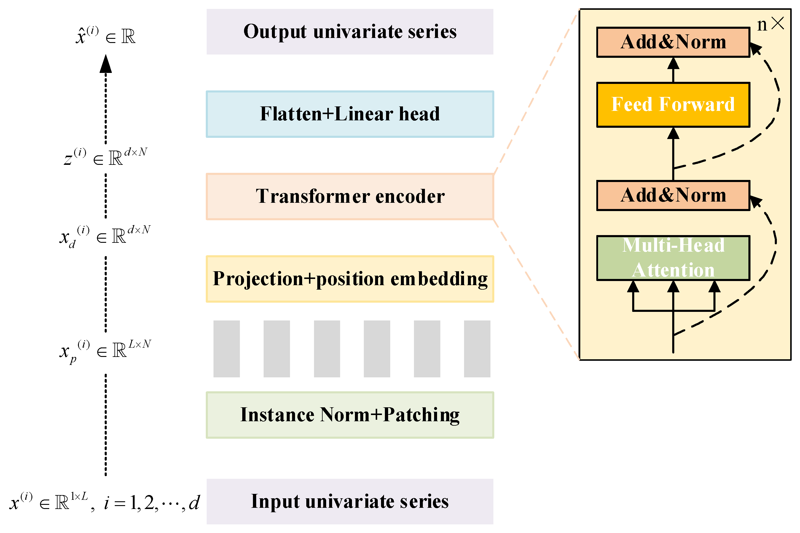
2.1. Patch Time Series Transformer

PatchTST is a time series modeling method based on the Transformer encoder. This method divides the sequence into several patch fragments by means of a sliding window, with each patch containing local information of a certain time length. The Transformer encoder extracts the dynamic dependencies between the patches, thereby achieving an accurate prediction of the future state [25]. In comparison with the conventional Transformer algorithm, PatchTST eschews the use of position encoding and instead relies on patch sequence modeling directly, a technique that boasts advantages such as simplicity, high accuracy, and adaptability [26]. The architecture of PatchTST is composed of the following key components [27], and its overall architecture is illustrated in Figure 1.

(1)

Patch Embedding

A multivariate time series $X=\left[x_1,x_2,\dots ,x_T\right]\in {ℝ}^{T\times d}$ of length $T$ and dimension $d$ is subjected to sliding window slicing to obtain $N$ patches:

$$X_{\mathrm{patch}}=\left[P_1,P_2,\dots ,P_N\right], P_i\in {ℝ}^L, N=T-L+1$$

(1)

Each patch is projected to a higher dimensional space by a linear transformation to form a patch representation matrix:

$$Z=X_{\mathrm{patch}}{W}^E+b^E, Z\in {ℝ}^{d\times N}$$

(2)

where $W^E\in {ℝ}^{d\times N}$ is the linear mapping matrix, $b^E\in {ℝ}^{d\times N}$ is the bias term, and $d$ is the embedding dimension.

(2)

Multi-head Self-Attention

The patch embedding matrix Z is used as input to the Transformer encoder, and the global dependencies between patches are first modeled by the multi-head self-attention mechanism, computed as:

$$\mathrm{Attention} (Q,K,V)=\mathrm{Softmax}\left({\displaystyle \frac{Q{K}^{\mathrm{T}}}{\sqrt{d_k}}}\right)V$$

(3)

$$\mathrm{MultiHead}(Q,K,V)=\mathrm{Concat}\left({\mathrm{head}}_1,\dots ,{\mathrm{head}}_h\right)W^O$$

(4)

$${\mathrm{head}}_i=\mathrm{Attention}\left(Z{W}_i^Q,Z{W}_i^K,Z{W}_i^V\right)$$

(5)

where $W_i^Q,W_i^K,W_i^V\in {ℝ}^{d\times d_k}$ and $W^O\in {ℝ}^{h{d}_k\times d}$ are the training parameters; h represents the number of attention heads.

(3)

Feed-forward Neural Network (FFN)

Each self-attention layer is followed by a feed-forward neural network module that performs a point-by-point nonlinear transformation of the feature vectors of each patch with the following formula:

$$FFN\left(x\right)=\max \left(0,x{W}_1+b_1\right)W_2+b_2$$

(6)

where $W_1\in {ℝ}^{d\times d_{ff}}$ and $W_2\in {ℝ}^{d_{ff}\times d}$ are the weight matrixes, $b_1$ and $b_2$ are the bias terms and $d_{ff}$ is the hidden layer dimension.

(4)

Residual Connection and Normalisation

To stabilize deep structure training, residual connections, and normalization operations are applied in the PatchTST algorithm after each sub-module (attention/FFN), as shown in the following expressions:

$$Output=LayerNorm\left[x+Sublayer\left(x\right)\right]$$

(7)

where $Sublayer\left(x\right)$ indicates the output of the attention module or FFN module.

(5)

Predictive Output Layer

The encoder outputs a representation vector of the last patch $z_{last}\in {ℝ}^d$ for the prediction of the next time step, and the output layer is a linear transformation:

$${\widehat{y}}_{T+1:}=z_{last}{W}^P+b^P$$

(8)

where $W^P\in {ℝ}^{d\times m}$ and $b^P\in {ℝ}^m$ denote parameters of the prediction layer.

In this study, the PatchTST framework is used to construct a multifactor-driven displacement prediction model for a single monitoring point of a concrete dam, which can effectively model the dynamic relationship between the input factors and achieve high-precision prediction of the single-point response.

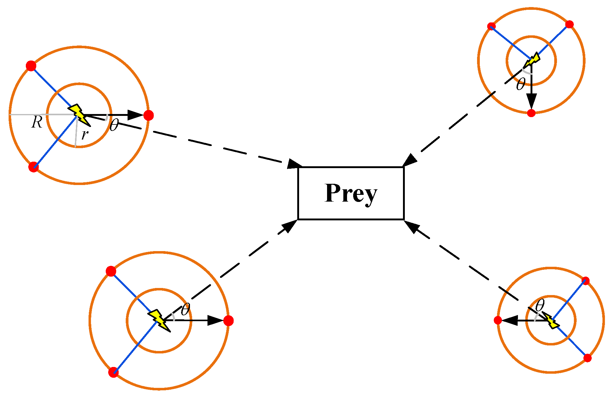
2.2. Sand Cat Swarm Optimization Algorithm

SCSO is a population intelligence optimization algorithm that simulates the foraging behavior of sand cats in the desert. The algorithm balances the global exploration and local exploitation ability of the population by dynamically adjusting the individual perception radius [28]. The schematic diagram of the position update of the sand cat population during the algorithm iteration is shown in Figure 2.

For the optimization problem with $D$ dimensional variables, it is assumed that there are $N$ sand cat individuals in the population, and the initialized population is:

$$X_{ij}=l{b}_j+r_0\left(u{b}_j-l{b}_j\right)$$

(9)

where $X_{ij}$ is the initial position of the i-th sand cat in the j-th dimension, i denotes an integer between 1~N, j is an integer between 1~D, $r_0$ represents a random number between 0 and 1, and $u{b}_j$ and $l{b}_j$ are the upper and lower boundaries of the j-th dimensional space, respectively.

Upon completion of the initialization process by the sand cat population, the hunting activity commences. The conversion factor R is utilized to determine whether the population proceeds to the search phase or the exploitation phase. The calculation of R is as follows:

$$R=2\cdot r_G\cdot rand\left(0,1\right)-r_G$$

(10)

where $r_G$ is the sensitivity factor, which can be calculated as:

$$r_G=S_M-\left(S_M\cdot ite{r}_c\right)/ite{r}_{\max }$$

(11)

where $ite{r}_c$ and $ite{r}_{\max }$ are the current iteration number and the maximum iteration number, respectively; $S_M$ is the hearing coefficient of sand cats, and the default value is 2 [29].

When $\left|R\right|>1$, the population enters the search phase. During this phase, the sand cat population updates its position in accordance with the current optimal solution and the current position of the population of individuals. At the (t + 1)-th iteration, the position of the i-th sand cat is updated by:

$$X_i\left(t+1\right)=r_i\cdot \left[X_{best}\left(t\right)-rand(0,1)\cdot X_i\left(t\right)\right]$$

(12)

where $X_{best}\left(t\right)$ is the optimal individual position of the sand cat population at the t-th iteration, $X_i\left(t\right)$ is the current position of the i-th sand cat, and $r_i=r_G\cdot rand\left(0,1\right)$.

When $\left|R\right|\le 1$, the sand cat enters the stage of attacking the prey, at this time the position of the i-th sand cat is updated by:

$$X_i\left(t+1\right)=X_{best}\left(t\right)-r_i\cdot X_{rand}\left(t\right)\cdot \cos \theta$$

(13)

$$X_{rand}\left(t\right)=\left|rand(0,1)\cdot X_{best}\left(t\right)-X_i\left(t\right)\right|$$

(14)

where $\theta$ is a random angle between 0°~360°.

2.3. Prediction Interval Construction Method Based on Quantile Regression

In the context of dam displacement monitoring, traditional point prediction methods are often inadequate for quantifying prediction uncertainty, which is inevitable due to uncertainties in the input data, external perturbations, and abrupt responses. To address these challenges, QR is employed in this study to construct upper and lower limits of prediction confidence intervals, with the aim of enhancing the assessment of the prediction results. QR seeks to estimate the conditional quantile of the target variable, that is, to predict the value of the output variable at a certain CL given the input characteristics. Let $y\in ℝ$ be the target value and ${\widehat{y}}^{\left(\tau \right)}\in ℝ$ be the predicted value of the $\tau \in \left(0,1\right)$-th quantile, then the loss function is defined as:

$${\mathcal{L}}_{\tau }(y,\widehat{y})=\left\{\begin{array}{ll}\tau (y-\widehat{y}),\hfill & \mathrm{if} y>\widehat{y}\hfill \\ (1-\tau )(\widehat{y}-y),\hfill & \mathrm{otherwise} \hfill \end{array}\right.$$

(15)

Specifically, if the 0.05-th quantile value ${\widehat{y}}^{\left(0.05\right)}$ and the 0.95-th quantile value ${\widehat{y}}^{\left(0.95\right)}$ are obtained by QR, the confidence interval of the predicted value at the significance level $\alpha =0.1$ can be constructed as $\left[{\widehat{y}}^{\left(0.05\right)},{\widehat{y}}^{\left(0.95\right)}\right]$. When $\tau =0.5$, Equation (15) degenerates into a loss function with the objective of minimizing the absolute error.

For the dam displacement prediction model based on the PatchTST algorithm constructed in this study, let the representation vector of the last patch output by the PatchTST encoder be $z_{last}\in {ℝ}^d$, then different quantiles can be predicted simultaneously by different linear mappings:

$${\widehat{y}}^{\left(\tau \right)}=z_{last}{W}^{\left(\tau \right)}+b^{\left(\tau \right)}$$

(16)

where $W^{\left(\tau \right)}\in {ℝ}^d$, $b^{\left(\tau \right)}\in ℝ$, and different $\tau$ values correspond to an independent set of parameters. For training, the objective function is the sum of all quantile losses:

$${\mathcal{L}}_{\mathrm{total}}={\displaystyle \sum _{k=1}^K{\mathcal{L}}_{{\tau }_k}(y,{\widehat{y}}^{\left({\tau }_k\right)})}$$

(17)

where $K$ is the number of total quantiles and ${\widehat{y}}^{\left({\tau }_k\right)}$ is the predicted value of the ${\tau }_k$-th quantile.

2.4. Shapley Additive Explanations

The dam displacement prediction model based on the PatchTST framework can help to capture the complex nonlinear mapping relationships in the time series monitoring data. However, this model is non-interpretable, which hinders the ability to intuitively understand the degree of influence of the factors on dam displacement. This is detrimental to the analyses and decision-making of engineering personnel. To address this problem, the influence of each factor on dam displacement is quantified in this study with the help of the SHAP method. In the SHAP method, the additive feature attribution strategy is used to interpret the output value of the PatchTST model as the sum of the effects of each input factor [30,31], i.e.:

$$g\left(z\right)={\varphi }_0+{\displaystyle {\sum }_{i=1}^m{\varphi }_i{z}_i}$$

(18)

where $g\left(z\right)$ is the explanatory model for the output values $\widehat{f}\left(x\right)$ of the SCSO-PatchTST model; $m$ denotes the number of input factors in the dam displacement prediction model; $z\in {\left\{0,1\right\}}^m$, and $z_i=1$ means that the variable $x_i$ exists in the SCSO-PatchTST model, whereas $z_i=0$ indicates its exclusion; ${\varphi }_0$ represents the constant term of the explanatory model, and ${\varphi }_i$ denotes the contribution of variable $x_i$ to $\widehat{f}\left(x\right)$, which is defined by the Shapley value in cooperative game theory. The mathematical expression of ${\varphi }_i$ is:

$${\varphi }_i={\displaystyle {\sum }_{S\subseteq \left\{x_1,x_2,\dots ,x_m\right\}/\left\{x_i\right\}}\frac{\left|S\right|!\left(m-\left|S\right|-1\right)!}{m!}}\left[\widehat{f}\left(S\cup \left\{x_i\right\}\right)-\widehat{f}\left(S\right)\right]$$

(19)

where $S$ denotes a subset of variable combinations, $\left\{x_1,x_2,\dots ,x_m\right\}/\left\{x_i\right\}$ is the set of all variables except $x_i$, and $\widehat{f}\left(S\right)$ represents the model output of the SCSO-PatchTST model built using only the variables contained in $S$.

As can be seen from Equation (19), the calculation of the Shapley value considers all possible combinations of variables that can constitute the model and averages the marginal contribution $\widehat{f}\left(S\cup \left\{x_i\right\}\right)-\widehat{f}\left(S\right)$ of the variable $x_i$ across these combinations, ensuring an objective assessment of its importance. The Shapley value is computed for individual predictions and reflects the local importance of a specific variable. The global importance of the variable $x_i$ then obtained by aggregating its local contributions over the training set, as expressed by:

$$I_i={\displaystyle {\sum }_{j=1}^N\left|{\varphi }_i^{\left(j\right)}\right|}/{\displaystyle \sum _{i=1}^m{\displaystyle \sum _{j=1}^N\left|{\varphi }_i^{\left(j\right)}\right|}}$$

(20)

where ${\varphi }_i^{\left(j\right)}$ denotes the local importance of variable $x_i$, calculated based on the model prediction corresponding to the j-th sample in the monitoring series.

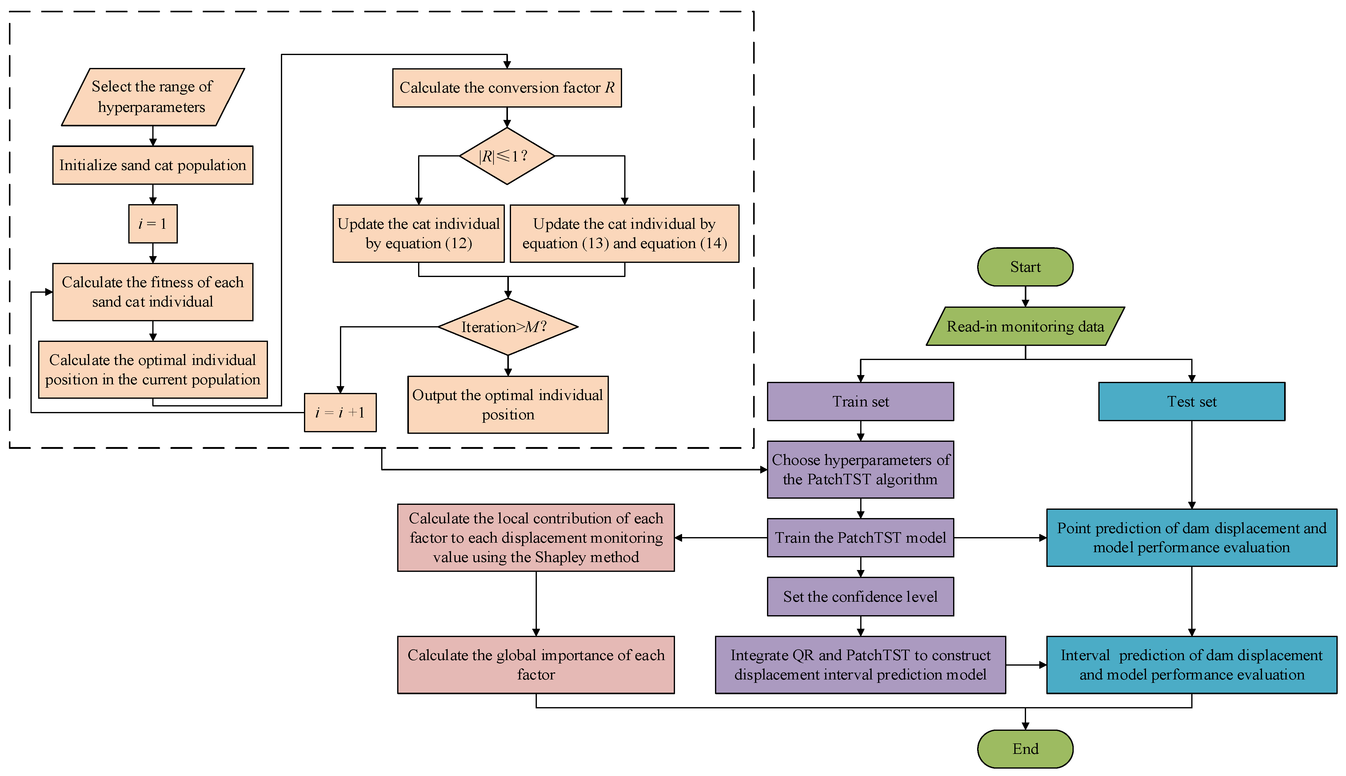
2.5. The Implementation Framework of the Proposed Method

Based on the above–mentioned theories, a deep learning approach that integrates PatchTST, QR, and SHAP for interval prediction of dam displacement is proposed, while also providing an interpretable analysis of the effects of influencing factors on dam displacement. The implementation framework of this method is illustrated in Figure 3.

3. Case Study

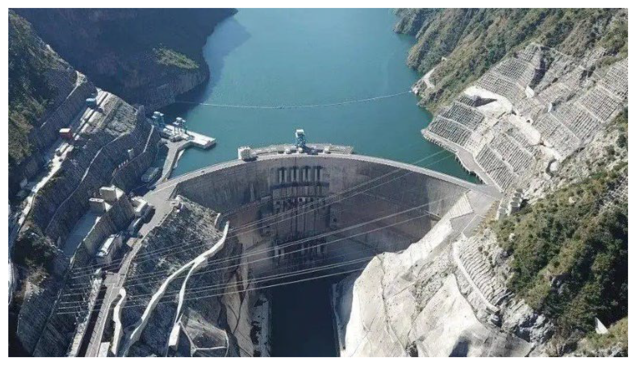
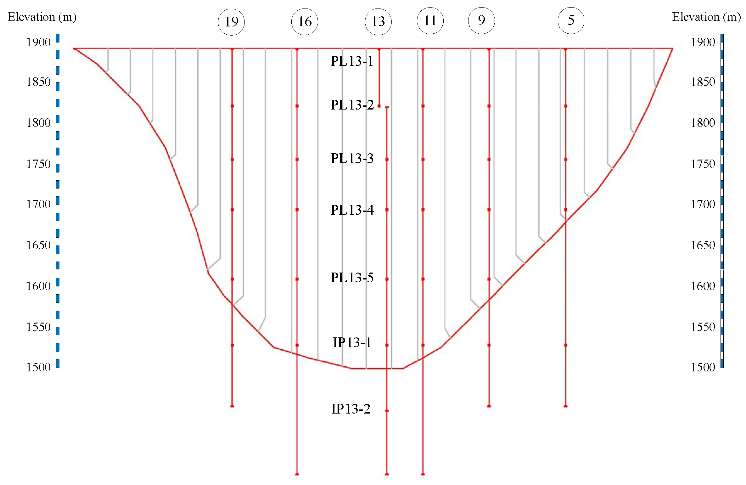
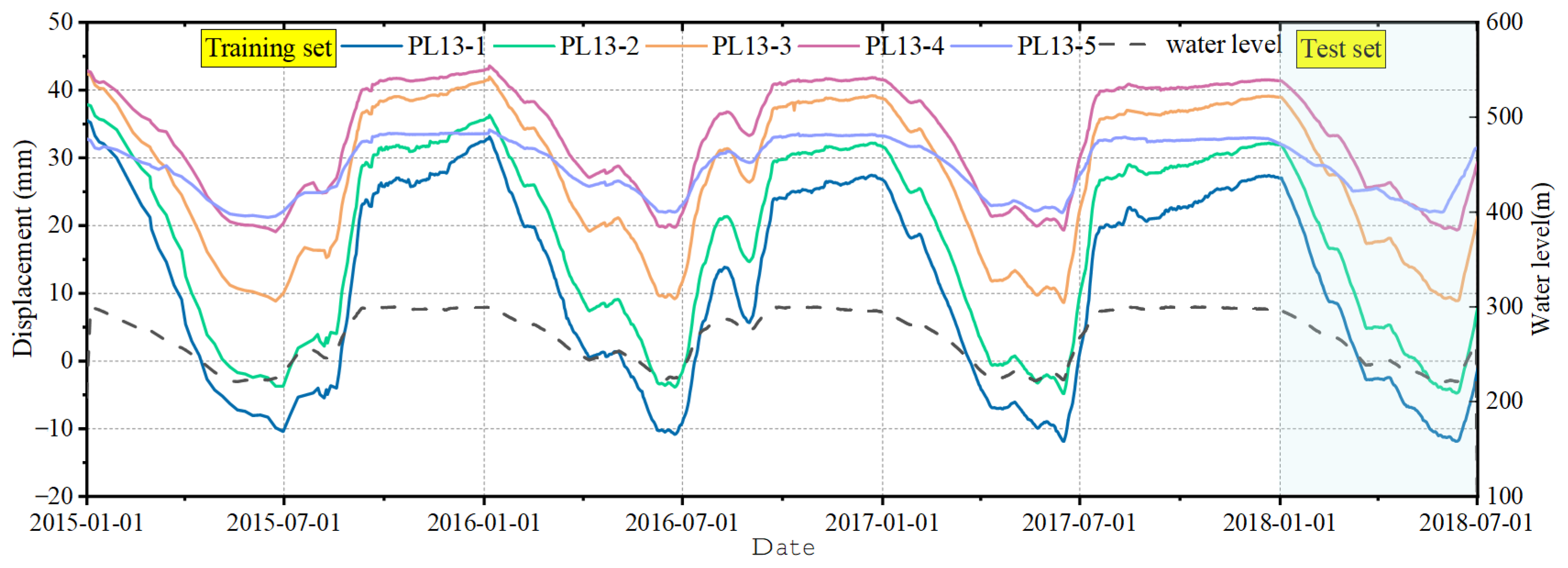
3.1. Engineering Introduction

In order to verify the effectiveness of the methodology proposed in this paper, a concrete double-curvature arch dam in Southwest China is used as an example to develop a case study in this study. The dam is located at the border of Yunnan and Sichuan provinces in China, and an aerial view of this dam is shown in Figure 4. The dam began impoundment in November 2012 and gradually reached the normal storage level in four stages by August 2014. Since then, it has remained in safe and stable operation. The normal storage level of this dam is 1880 m and the maximum height of the dam is 305 m.

In order to monitor the radial displacements of the dam, several plumb lines (PLs) and inverse plumb lines (ILs) are arranged in the downstream face of the dam at dam sections 5, 9, 11, 13, 16, and 19, respectively, as shown in Figure 5. The plumb line (PL) is used to measure the relative radial displacement between adjacent monitoring points, while the inverted plumb line (IP) is employed to measure the relative radial displacement between a monitoring point and an anchoring point located deep within the dam foundation, which is assumed to remain stationary. Therefore, the IP can be regarded as providing absolute radial displacement. By combining measurements from both PL and IP systems, the absolute radial displacement of each monitoring point relative to the fixed point in the deep foundation can be determined. It should be noted that all dam radial displacement data presented in the following sections are absolute radial displacements derived from the processing of original measurements. Each plumb line includes multiple monitoring points, and the layout of the monitoring points on the plumbline system for dam section No. 13 in this case study is also shown in Figure 5.

The process lines of the radial displacement of the dam section 13, measured by five monitoring points in the plumbline system, are shown in Figure 6. Combining Figure 5 and Figure 6 reveals that the radial displacement of the dam section 13 exhibits a general trend of larger middle and smaller ends, with the amplitude of displacement fluctuation being directly proportional to the elevation of the monitoring points. Among these, the annual variation of the monitoring points PL13-1 and PL13-2 is the most significant. Consequently, the present study utilizes the monitoring data from these two points as a basis for constructing a displacement prediction model. The monitoring data from 1 January 2015 to 31 December 2017 was utilized as the train set, while the monitoring data from 1 January 2018 to 30 June 2018 was employed as the test set. During the initial period, the monitoring frequency was approximately once a week, whereas in the subsequent period, it was approximately once a day. The train set for monitoring points PL13-1 and PL13-2 comprises approximately 870 monitoring data points, while the test set contains approximately 180 monitoring data points.

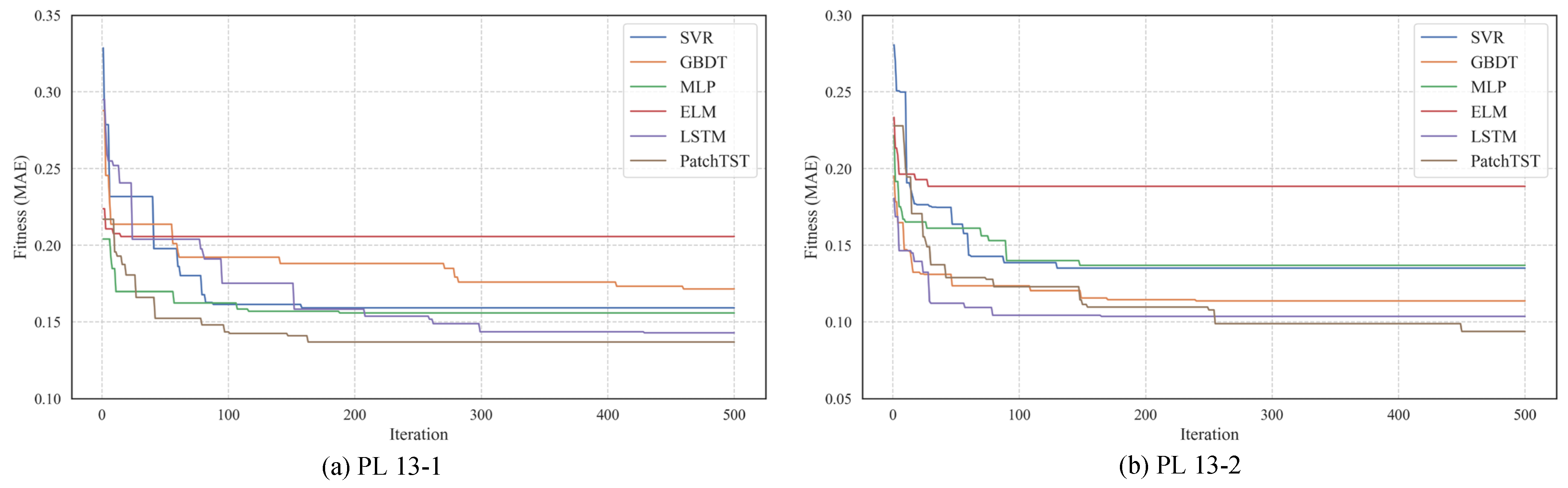
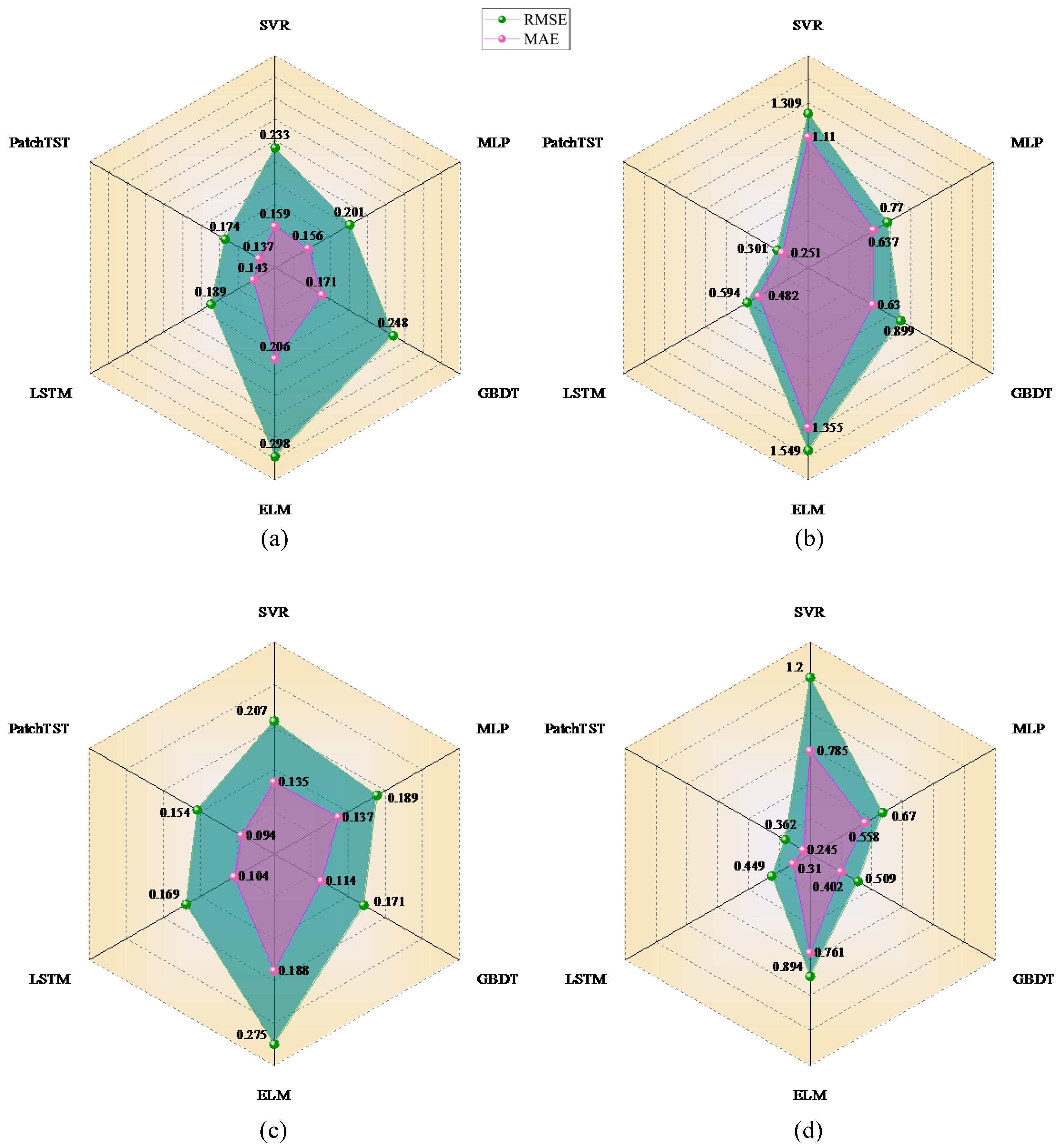
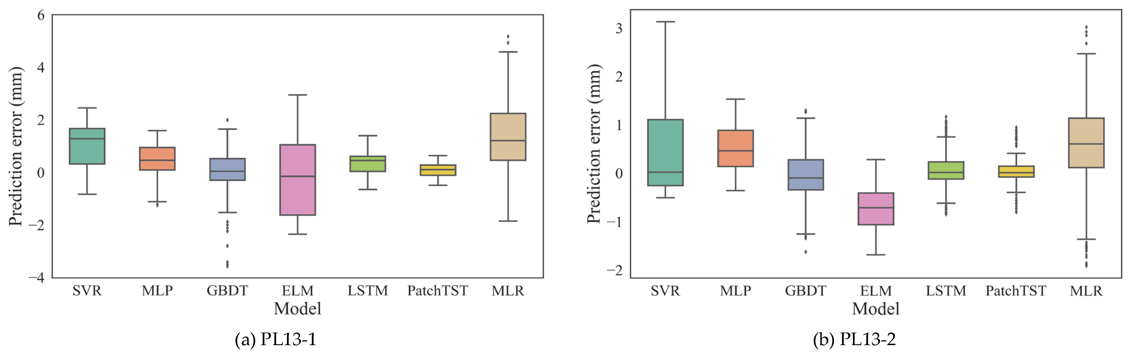
3.2. Point Prediction of Dam Displacement

According to the previous research results, the displacement of any point in a concrete dam is related to factors such as water pressure, temperature loading, and time-dependent creep properties of the material, so the construction of the displacement prediction model for concrete dams can be referred to traditional hydraulic, seasonal, and time (HST) causal factors-based statistical model.

Due to the importance of dam safety, certain safety margins are typically reserved in engineering design. Previous studies have shown that under normal operating conditions, most regions of a concrete dam remain in an elastic state [32]. Therefore, in this study, the dam displacement caused by hydrostatic pressure is assumed to be primarily related to the current-day water load, and the lag effect is not explicitly considered. In contrast, for temperature loads, it has been widely acknowledged that there exists a significant lag effect due to the time required for heat conduction within the concrete [33]. This indicates a phase lag between the ambient temperature variation and the resulting thermal-induced dam displacement. In this study, temperature-related influencing factors are approximately represented using harmonic factors [34]. On one hand, trigonometric functions can capture the annual periodic pattern of temperature variations effectively. On the other hand, a linear combination of sine and cosine functions can approximate harmonic functions with arbitrary phase shifts, thereby implicitly incorporating the lag effect of thermal loads. As for time-dependent displacement, its occurrence is primarily associated with the creep behavior of the concrete dam and the foundation rock. This displacement mechanism is relatively complex. Based on previous studies [7], incorporating both the time term and the logarithmic term of time as time-dependent factors has been shown to yield satisfactory fitting performance.

Therefore, in this study, the influencing factors of dam displacement are defined as follows:

$$I_{input}=\left\{H-H_0,H^2-H_0^2,H^3-H_0^3,H^4-H_0^4,\sin {\displaystyle \frac{2\pi t}{365}},\cos {\displaystyle \frac{2\pi t}{365}},\sin {\displaystyle \frac{4\pi t}{365}},\cos {\displaystyle \frac{4\pi t}{365}},{\displaystyle \frac{t}{100}},\ln {\displaystyle \frac{t}{100}}\right\}$$

(21)

where $H$ represents the upstream water depth, $H_0$ denotes the upstream water depth at the initial monitoring day, $t$ is the cumulative number of days since the initial monitoring day.

The factors shown in Equation (21) are used as the input factors, and the dam displacement monitoring data are used as the output variables to construct the dam displacement prediction model at the monitoring points PL13-1 and PL13-2 based on the PatchTST algorithm. In the PatchTST algorithm, the number of attention head size (n_heads), model dimension (d_model), the learning rate (learning_rate), and the batch size (batch_size) have a significant effect on the performance of the model. These parameters are used as hyperparameters to be optimized in this study. In order to facilitate the comparison of the prediction results of the PatchTST model, several comparative models that have been proven to have good performance in dam displacement prediction are also considered in this study, including SVR [35], LSTM [36], gradient boosting decision tree [37] (GBDT), multilayer perceptron (MLP) [38] and extreme learning machine (ELM) [39]. For SVR, the penalty parameter (C) and kernel coefficient (γ) are the key hyperparameters. For LSTM, the number of layers (num_layers), the number of neurons per layer (units), and the learning rate are optimized. In GBDT, the number of decision trees (n_estimators), maximum tree depth (max_depth), learning rate, and sample proportion per tree (subsample) are considered. The MLP model is controlled by the number of hidden layers and the learning rate. While in ELM, the only tunable hyperparameter is the number of hidden layer nodes (L). All models are trained on the same dataset using identical input and output variables. The initial search ranges for each model’s hyperparameters are listed in

Table 1. Parameter optimization results.

Model	Hyperparameters	Initial Range	Optimal Parameter
			PL13-1	PL13-2
PatchTST	n_heads	[2, 8]	5	4
	d_model	[32, 256]	128	128
	learning_rate	[0.0001, 0.01]	1.12 × 10−3	6.45 × 10−4
	batch size	[16, 128]	32	64
SVR	C	[10−3, 103]	128.48	156.39
	γ	[10−3, 1]	4.75 × 10−3	1.36 × 10−3
LSTM	units	[32, 256]	128	256
	num_layers	[1, 3]	2	2
	learning_rate	[0.0001, 0.01]	1.23 × 10−3	7.12 × 10−4
GBDT	n_estimators	[100, 1000]	299	813
	learning_rate	[0.01, 0.5]	8.82 × 10−2	2.13 × 10−1
	max_depth	[3, 10]	4	5
	subsample	[0.5, 1]	9.73 × 10−1	9.38 × 10−1
MLP	num_layers	[10, 500]	89	105
	learning_rate	[0.0001, 0.01]	5.40 × 10−3	1.91 × 10−2
ELM	L	[10, 500]	351	216

.

The SCSO algorithm is then employed to optimize and solve the hyperparameters in each model. The number of sand cat populations is set at 30 and the maximum number of iterations in the SCSO algorithm is set at 500. The average absolute error (MAE) between the fitted values and the actual values in the train set is taken as the objective function. To prevent overfitting, five-fold cross-validation is applied during the optimization process, and the average error across the folds is used as the final evaluation metric. The optimization process of each model is illustrated in Figure 7, and the outcomes of parameter optimization are also presented in Table 1.

As illustrated in Figure 7, all models exhibit a marked reduction in MAE during the first 100 iterations. With increasing iterations, most models tend to converge after approximately 200 iterations, where the MAE values show little further decrease. This indicates that the SCSO algorithm possesses strong initial exploratory capabilities in the parameter space, enabling rapid performance improvement and demonstrating good convergence characteristics.

In addition to the six machine learning models mentioned above, a traditional multiple linear regression (MLR) model, which establishes a linear mapping between the input factors and dam displacement monitoring values using the least squares method, is also introduced for comparison. The performance of the models on both the training and test sets is summarized in

Table 2. Performance evaluation results of dam displacement prediction models.

Monitoring Points	Model	Train Set			Test Set
		RMSE	MAE	R2	RMSE	MAE	R2
PL 13-1	MLR	1.413	1.134	0.989	1.865	1.584	0.973
	SVR	0.233	0.159	1.000	1.309	1.110	0.987
	MLP	0.201	0.156	1.000	0.770	0.637	0.995
	GBDT	0.248	0.171	1.000	0.899	0.630	0.994
	ELM	0.298	0.206	1.000	1.549	1.355	0.982
	LSTM	0.189	0.143	1.000	0.594	0.482	0.997
	PatchTST	0.174	0.137	1.000	0.301	0.251	0.999
PL 13-2	MLR	0.936	0.712	0.995	1.124	0.963	0.99
	SVR	0.207	0.135	1.000	1.200	0.785	0.988
	MLP	0.189	0.137	1.000	0.670	0.558	0.996
	GBDT	0.171	0.114	1.000	0.509	0.402	0.998
	ELM	0.275	0.188	1.000	0.894	0.761	0.994
	LSTM	0.169	0.104	1.000	0.449	0.310	0.998
	PatchTST	0.154	0.094	1.000	0.362	0.245	0.999

, where the evaluation metrics include the mean absolute error (MAE), root mean square error (RMSE), and coefficient of determination (R²), with their respective computational formulas provided below. The optimal values for each performance metric in Table 2 are highlighted in bold.

$$MAE={\displaystyle \frac{1}{n}}{\displaystyle \sum _{i=1}^n\left|y_i-{\widehat{y}}_i\right|}$$

(22)

$$RMSE=\sqrt{{\displaystyle \frac{1}{n}}{\displaystyle \sum _{i=1}^n{\left|y_i-{\widehat{y}}_i\right|}^2}}$$

(23)

$$R^2=1-{\displaystyle \frac{{\displaystyle \sum _{i=1}^n{\left(y_i-{\widehat{y}}_i\right)}^2}}{{\displaystyle \sum _{i=1}^n{\left(y_i-\overline{y}\right)}^2}}}$$

(24)

where $y_i$ and ${\widehat{y}}_i$ are the measured and predicted values of the i-th sample in the dam displacement monitoring data, respectively, and n is the number of samples in the train or test set.

As shown in Table 2, among all seven models, the traditional MLR model exhibits the worst performance at both monitoring points, especially on the train set. This highlights the necessity of using nonlinear models to learn the mapping relationship between influencing factors and dam displacement measurements. Nevertheless, the coefficient of determination (R²) remains consistently above 0.97 across all datasets, indicating that the influencing factors listed in Equation (21) possess a high level of generalization in explaining the causes of dam displacement. To enable a more intuitive comparison of the predictive capabilities among the six machine learning models, radar charts illustrating the performance metrics RMSE and MAE across different monitoring points and datasets are presented in Figure 8.

Integrating the results from Figure 8 and Table 2, the PatchTST model consistently outperforms all other models at both monitoring points PL13-1 and PL13-2. It achieves the lowest RMSE and MAE on both the train and test sets, while the coefficient of determination (R²) reaches the highest level (1.000 and 0.999, respectively). These results highlight the superior predictive accuracy and stability of the PatchTST model in capturing the temporal characteristics of dam displacement. The LSTM model ranks second, with RMSE values of 0.594 mm and 0.449 mm, and MAE values of 0.482 mm and 0.310 mm on the test set of PL13-1 and PL13-2, respectively. These results are significantly better than those of traditional machine learning models such as SVR, ELM, MLP, and GBDT, underscoring the remarkable advantage of deep learning models in the task of dam displacement prediction.

Among machine learning methods, the MLP and GBDT models yield comparable results on the test sets. However, SVR and ELM demonstrate relatively poor performance, likely due to their simpler architectures, which are insufficient to capture the complex patterns inherent in the data. Nevertheless, after parameter tuning using the SCSO algorithm, R² values of all six models achieve above 0.98 on the test sets, with maximum RMSE and MAE not exceeding 1.55 mm and 1.36 mm, respectively. These findings confirm that the input factors identified in Equation (21) effectively encapsulate the mechanisms underlying dam displacement and that the resulting predictive models possess considerable practical value. Additionally, a comparison of fitting and predicting performance reveals that all models attain noticeably higher accuracy on the train sets, indicating varying degrees of overfitting during model training. This issue is particularly pronounced in traditional machine learning models, whose performance deteriorates more significantly on the test set. In contrast, the PatchTST and LSTM models demonstrate superior generalization capability and robustness.

To further visualize the predictive performance of each model on the test sets, boxplots of prediction errors are presented in Figure 9. In these plots, the upper and lower edges of the boxes represent the third and first quartiles, respectively; the line within each box denotes the median prediction error; the whiskers indicate error ranges within 1.5 times the interquartile range; and outliers are shown as black dots. From Figure 9, it is evident that both the PatchTST and LSTM models produce relatively small prediction errors with compact box distributions, indicating high prediction accuracy and good stability. Notably, the PatchTST model exhibits even more concentrated box ranges and smaller error fluctuations. Its median prediction errors at both PL13-1 and PL13-2 are closer to zero, further highlighting its outstanding performance in terms of both accuracy and robustness.

Regarding the remaining five models, at the PL13-1 monitoring point, the MLP and GBDT models yield similar box widths, but the GBDT model displays more dispersed error distributions with some outliers, suggesting potential localized prediction failures. The ELM model exhibits the widest box, while the MLR model shows the most extensive distribution of prediction errors, indicating that both models suffer from the lowest predictive accuracy and limited stability among all models. At the PL13-2 monitoring point, the trends are consistent with those at PL13-1. However, the SVR model presents the widest box, whereas the MLR model still displays the most dispersed error distribution. Considering the performance across both monitoring points, the MLR model, which is characterized by its inherent linear structure, demonstrates the poorest prediction stability among all comparative models, followed by the SVR and ELM models.

In summary, the boxplot analysis in Figure 9 is in strong agreement with the model performance metrics reported in Table 2. These results from both distributional and numerical perspectives robustly demonstrate the superior performance of the proposed SCSO-PatchTST model in predicting radial displacement of the concrete dam. The excellent results of the SCSO-LSTM model further affirm the reliability and strong generalization ability of deep learning approaches in dam displacement prediction tasks.

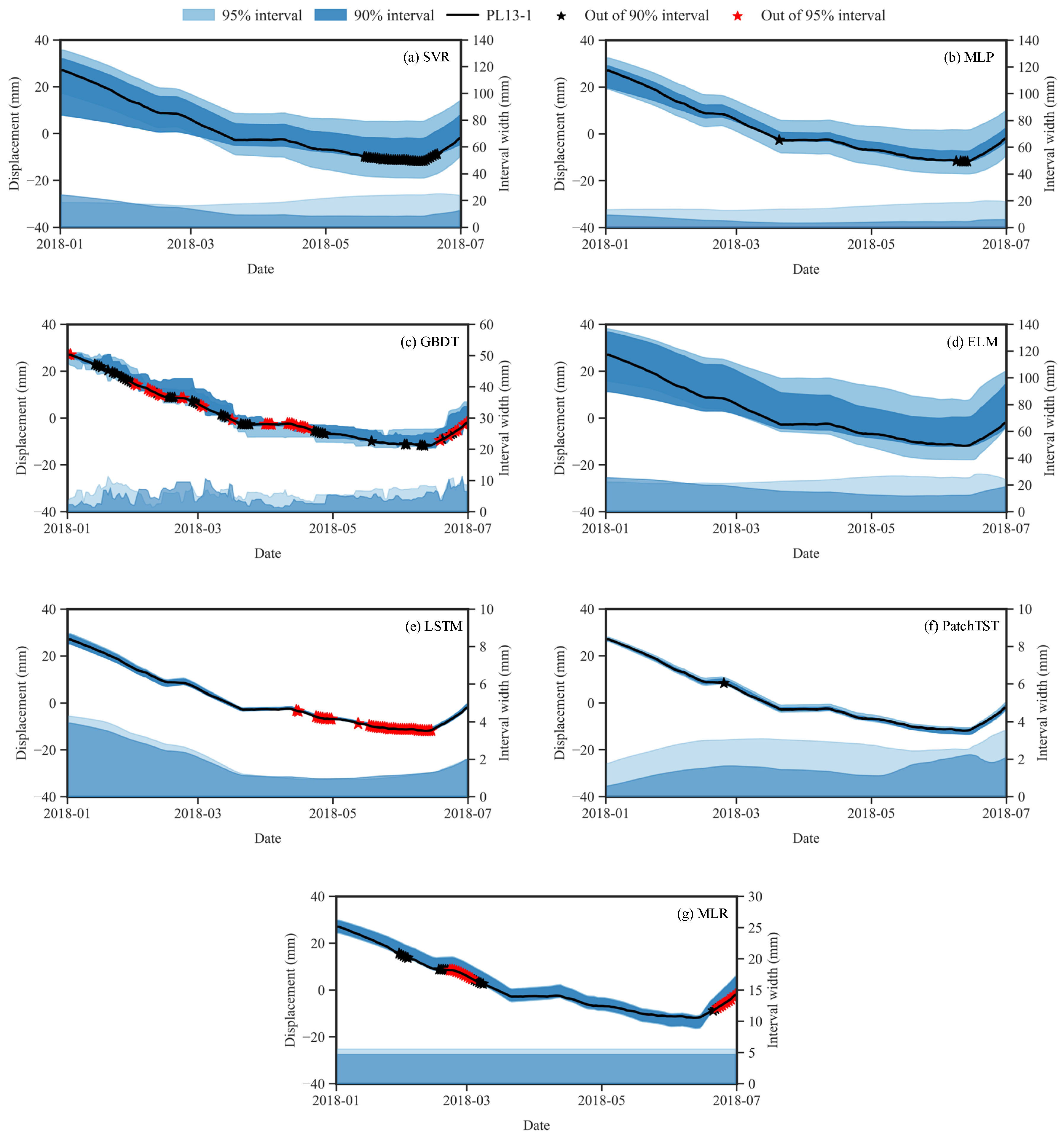
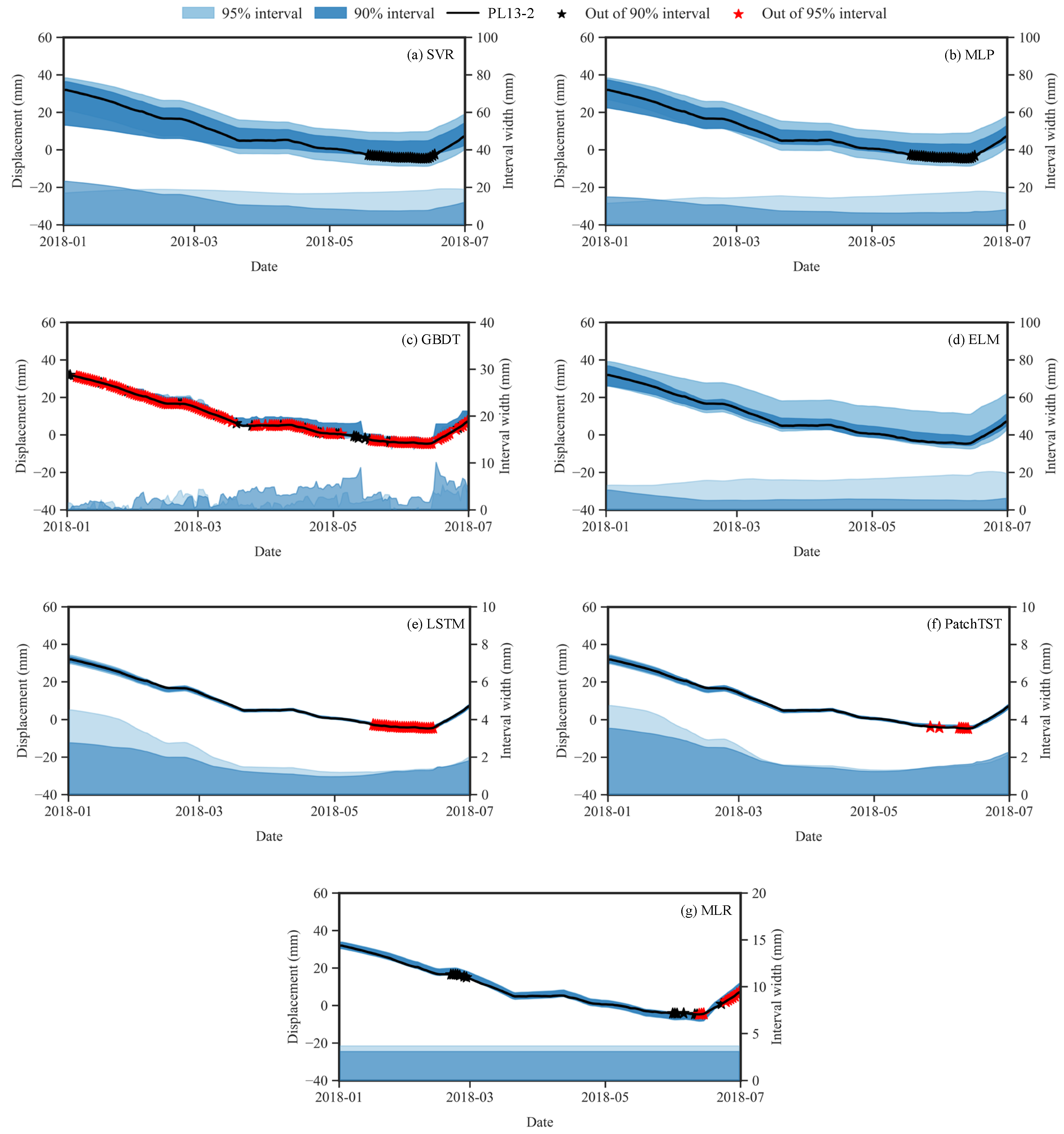
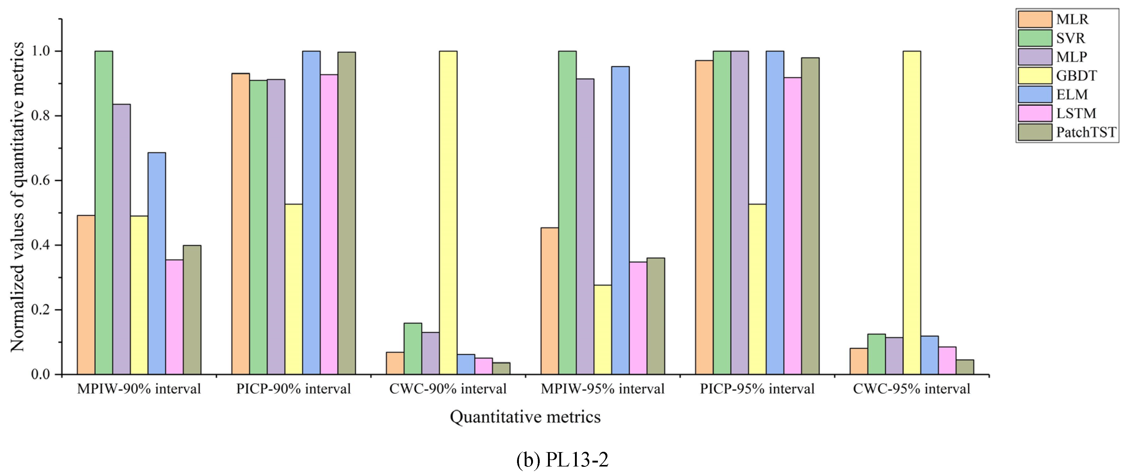
3.3. Interval Prediction of Dam Displacement

Based on the optimized parameters reported in Table 1, the PatchTST model and five other machine learning-based comparative models were trained using the train sets from monitoring points PL13-1 and PL13-2. PIs were then constructed using the QR method described in Section 2.3. Two CLs, 90% and 95%, were considered in this study. For the MLR model, by contrast, PIs were generated using the traditional confidence interval approach defined as $\left[{\widehat{y}}_i-k\sigma ,{\widehat{y}}_i+k\sigma \right]$, where $\sigma$ denotes the standard deviation of the prediction errors. The coefficient $k$ is set to 1.645 and 1.960 for CLs of 90% and 95%, respectively.

The PI construction results of the seven models on the test sets are illustrated in Figure 10 and Figure 11, respectively. In each figure, the black solid line represents the observed radial displacement of the dam; the light blue shaded area denotes the 95% PI, while the dark blue area corresponds to the 90% PI. The upper part of each figure shows the predicted displacement intervals, whereas the lower part depicts the corresponding interval widths, aligned with the secondary y-axis on the right. Black asterisks indicate measured displacement falling outside the 90% PI but within the 95% PI, while red asterisks mark those exceeding the 95% PI.

According to the dam’s actual operational records, no significant anomalies occurred during the period covered by this case study, indicating stable performance. Hence, the measurements at PL13-1 and PL13-2 are considered reliable, and any observed deviation from the PIs can be treated as false alarms. From the PI results shown in Figure 10 and Figure 11 for PL13-1 and PL13-2, it is evident that there are substantial differences among models in terms of both interval width and coverage performance. Notably, the PatchTST and LSTM models produce narrow and stable PIs, with widths generally maintained below 4 mm throughout the predicting period. Compared to LSTM, the PatchTST model achieves a lower false alarm rate while maintaining a comparable interval width. According to the prediction results of the PatchTST model, only one data point at PL13-1 falls outside the 90% PI, while seven such points are identified as false alarms at PL13-2. The PI width of the MLR model is slightly greater than those of the LSTM and PatchTST models. Due to the limitations of the traditional construction method, the PI width remains constant across all measurements and thus fails to reflect the variability of prediction uncertainty. Moreover, despite the relatively wide PIs, the MLR model exhibits a significantly higher false alarm rate compared to the PatchTST model, with 37 and 24 measurements falling outside the 90% PI at monitoring points PL13-1 and PL13-2, respectively.

In contrast, the other four machine learning-based models generate significantly wider PIs. The 95% PIs constructed by SVR, MLP, and ELM, for example, approach widths of nearly 20 mm. Although wider intervals can improve coverage probabilities, they also indicate greater predictive uncertainty. Moreover, despite these wider intervals, SVR, MLP, and GBDT exhibit higher false alarm rates compared to the PatchTST model. Particularly noteworthy is the GBDT model, which exhibits evident prediction failure at both monitoring points. At PL13-2, the vast majority of observations fall outside the 95% PI, and the interval width exhibits pronounced fluctuations, further confirming the limitations of the model in the current application scenario.

To objectively evaluate the interval prediction performance of each model, three quantitative metrics were adopted in this study: the Mean Prediction Interval Width (MPIW), the Prediction Interval Coverage Probability (PICP), and the Coverage Width-based Criterion (CWC). MPIW reflects the average width of the PIs on the test set, while PICP and CWC are computed using the following formulas:

$$\mathrm{PICP}={\displaystyle \frac{1}{n}}{\displaystyle \sum _{i=1}^n{\epsilon }_i}, {\epsilon }_i=\left\{\begin{array}{c}1,y_i\in \left[L_i, U_i\right]\\ 0,y_i\notin \left[L_i, U_i\right]\end{array}\right.$$

(25)

$$\mathrm{CWC}=\left[{\displaystyle \frac{1}{n}}{\displaystyle \sum _{i=1}^n\left(U_i-L_i\right)}\right]\cdot \left[1+\gamma \cdot \exp \left(-\eta \cdot \left(\mathrm{PICP}-\mu \right)\right)\right], \gamma =\left\{\begin{array}{c}1, \mathrm{PICP}<\mu \\ 0, \mathrm{PICP}\ge \mu \end{array}\right.$$

(26)

where $n$ is the length of the test set, $U_i$ and $L_i$ are the upper and lower PI bounds of the i-th observed displacement in the test set, respectively, μ represents the CL, and η is a penalty coefficient, typically set to a relatively large value. Following the reference literature [40], the penalty coefficient η was set to 10 in this study. The CWC comprehensively evaluates both coverage probability and interval width. When the PICP reaches the predefined CL μ, CWC is equal to the MPIW; otherwise, CWC exceeds MPIW. According to its definition, an ideal PI model should yield a relatively low MPIW, a high PICP, and consequently a low CWC.

The interval prediction results of the six models at both monitoring points are summarized in

Table 3. Evaluation results of interval predictions for dam displacement using different models based on quantile regression.

Monitoring Points	Model	90% Interval			95% Interval
		MPIW	PICP	CWC	MPIW	PICP	CWC
PL 13-1	MLR	4.669	0.794	18.145	5.562	0.889	15.798
	SVR	12.435	0.811	42.714	19.948	1.000	19.948
	MLP	5.142	0.967	5.142	15.365	1.000	15.365
	GBDT	4.802	0.689	44.410	6.157	0.811	30.848
	ELM	16.854	1.000	16.854	23.783	1.000	23.783
	LSTM	1.833	0.806	6.525	1.955	0.778	12.873
	PatchTST	1.469	0.994	1.469	2.758	1.000	2.758
PL 13-2	MLR	3.093	0.867	7.395	3.685	0.944	7.598
	SVR	12.779	0.828	39.033	17.895	1.000	17.895
	MLP	8.922	0.833	26.358	14.971	1.000	14.971
	GBDT	3.068	0.278	1545.362	1.372	0.278	1141.050
	ELM	6.011	1.000	6.011	16.232	1.000	16.232
	LSTM	1.606	0.861	3.978	2.165	0.844	8.385
	PatchTST	2.035	0.994	2.035	2.328	0.961	2.328

. Similarly, to provide a more intuitive comparison of the interval prediction performance, the evaluation results in Table 3 were square-root transformed and then normalized based on the maximum value of each indicator at each monitoring point. The resulting normalized metrics for all models are presented in the form of bar charts in Figure 12. A general trend is evident in which the PatchTST model outperforms the others under both CLs and at both monitoring points. It yields relatively low MPIW values, indicating tighter intervals, and its PICP values reach the target CL, reflecting excellent coverage. Specifically, the PatchTST model achieves MPIW values of 2.758 mm and 2.328 mm at PL13-1 and PL13-2, respectively, under the 95% CL, slightly higher than those of the LSTM model. Similarly, the LSTM model also exhibits strong interval prediction capability, with comparatively low MPIW values and significantly lower CWC scores than traditional machine learning models. However, its PICP under the 95% CL fails to reach the target level, with values of only 0.778 and 0.844 at PL13-1 and PL13-2, respectively, suggesting that under certain conditions, the LSTM model may still exhibit slight undercoverage.

By contrast, traditional machine learning models perform relatively poorly. For instance, the PICP of the GBDT model at both monitoring points is significantly below the expected CL, with a particularly low PICP value of 0.278 at PL13-2 under the 90% CL. The corresponding CWC reaches as high as 1545.362, indicating severe failure in constructing valid and effective PIs. Although the SVR and MLP models meet the required PICP thresholds under the 95% CL, their intervals are excessively wide, resulting in high CWC values and thus reduced practical utility. Notably, the ELM model, despite achieving a perfect PICP of 1.000 on both the train and test sets at both monitoring points, produces the highest MPIW among all models. This indicates that its high coverage is obtained at the cost of excessively wide intervals, which may lead to overly conservative predictions and poor sensitivity to abnormal behavior. For the MLR model, although the confidence intervals constructed using the traditional method exhibit relatively acceptable widths, the PICP values consistently fall short of the nominal levels under all tested conditions. This may be attributed not only to the model’s limited ability to capture the nonlinear characteristics of dam displacement but also to the limitations of the conventional interval construction approach itself. Specifically, this method relies on assumptions of homoscedasticity and normally distributed errors, which may not hold in practice. Consequently, it may struggle to accommodate local variations in prediction uncertainty, thereby reducing the reliability and adaptability of the resulting PIs in complex monitoring scenarios.

It should be noted that although the proposed SCSO-PatchTST-QR model demonstrates strong performance in interval prediction, it still cannot entirely eliminate the occurrence of false alarms. The dam displacement anomaly identification method based on this interval prediction model is fundamentally grounded in statistical principles. It serves as a preliminary screening tool to identify potentially abnormal deformation measurements within a given confidence interval. When applying the SCSO-PatchTST-QR model to dam safety monitoring and early warning, the anomalies identified by the model should be further evaluated in conjunction with the actual operational conditions of the dam (e.g., signs of leakage or abnormal vibrations) and the anomaly detection results across multiple monitoring points. Such a comprehensive assessment is essential for achieving accurate early warning of potential dam operation risks.

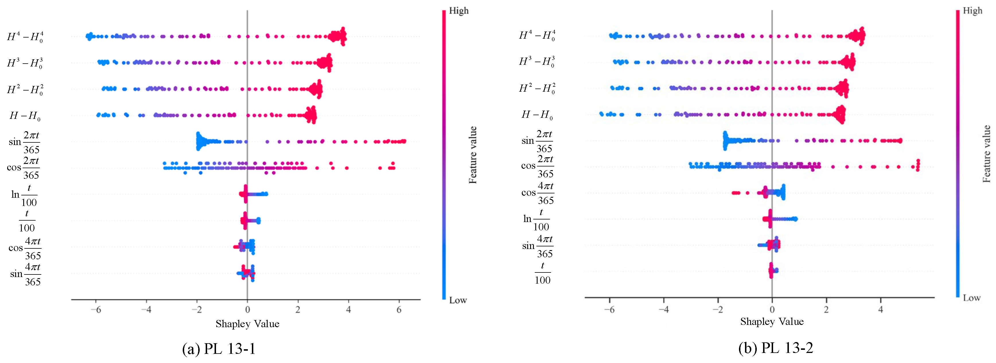
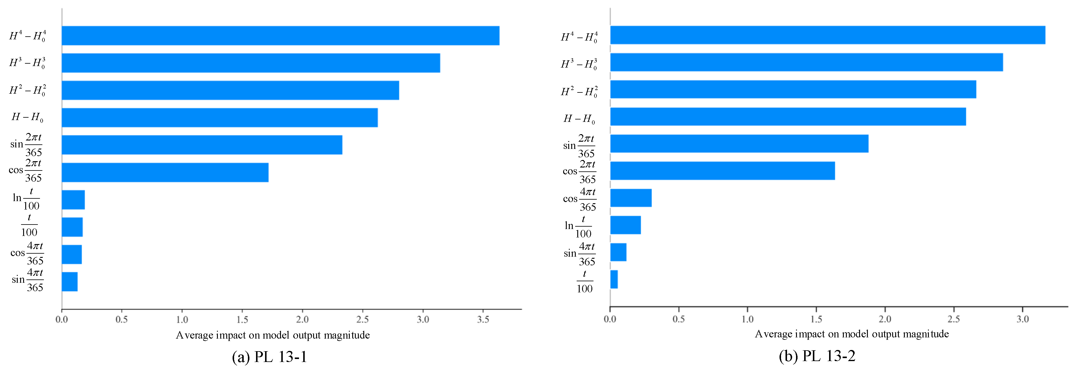
3.4. Analysis of Dam Displacement Driving Mechanism

The aforementioned results from point prediction and PIs jointly demonstrate the superior performance of the proposed SCSO-PatchTST model in dam displacement prediction. To further interpret the physical implications of the model predictions and uncover the driving mechanism behind input features, the SHAP method introduced in Section 2.4 is employed to quantify the importance of each input factor in Equation (21) and its directional impact on the model output. Specifically, 100 samples were randomly selected from the training dataset, and the Shapley values of each input variable were computed based on Equation (19), resulting in a total of 100 Shapley values per variable. These values were visualized in the summary scatter plot shown in Figure 13. In this plot, each point represents the Shapley value of a specific feature for a single sample, where the horizontal axis denotes the magnitude and direction of that feature’s contribution to the predicted displacement, and the vertical axis lists the features in descending order of global importance. The color of each point reflects the actual value of the corresponding feature in the train set—red indicates a high feature value, while blue indicates a low value. Furthermore, the global importance of each input factor was evaluated by calculating the mean absolute Shapley value using Equation (20), and the results were presented in the bar chart shown in Figure 14, which provides an aggregated view of the contribution of each variable to the model output across all selected samples.

As shown in Figure 13 and Figure 14, the dominant influencing factors identified by the model outputs are highly consistent across the two monitoring points. The results indicate that the most significant factor affecting the radial displacement of the arch dam is related to water pressure variation, followed by trigonometric function terms representing temperature fluctuations. In contrast, the time-dependent deformation caused by concrete and rock creep has a relatively limited impact. This suggests that the radial displacement of the dam is primarily governed by the loading and unloading effects of water pressure, while the thermal expansion and contraction induced by environmental temperature variation play a secondary role.

Among the key influencing factors, those with red Shapley values are mainly concentrated in the positive range, while those with blue Shapley values are primarily in the negative range, indicating that water level rise contributes positively to the increase in radial displacement which means the downstream deformation of the dam. It is important to note that the trigonometric terms simulate the periodic pattern of temperature variation rather than actual concrete temperature values. The radial displacement exhibits a significant positive correlation with both $\sin {\displaystyle \frac{2\pi t}{365}}$ and $\cos {\displaystyle \frac{2\pi t}{365}}$ with similar levels of correlation for the two components. In contrast, the relatively weak correlation with the semi-annual terms $\sin {\displaystyle \frac{4\pi t}{365}}$ and $\cos {\displaystyle \frac{4\pi t}{365}}$ suggests that the temperature-induced dam displacement primarily follows an annual cycle. Moreover, the periodic impact of temperature on radial displacement lies between $\sin {\displaystyle \frac{2\pi t}{365}}$ and $\cos {\displaystyle \frac{2\pi t}{365}}$, suggesting that during certain time periods between January and March, temperature contributes most significantly to downstream deformation, while this effect diminishes during certain periods from June to September. Considering the annual temperature cycle in Southwest China, it can be inferred that lower winter temperatures lead to thermal contraction and downstream displacement of the concrete, while higher summer temperatures result in upstream displacement due to thermal expansion. Therefore, the importance attribution results based on the SCSO-PatchTST model and SHAP method are consistent with the general physical laws governing dam displacement under water level and temperature effects, validating the ability of the SCSO-PatchTST model to capture the underlying variation pattern of radial displacement.

4. Conclusions and Future Discussions

In this study, an integrated deep learning framework—SCSO-PatchTST—was developed to advance dam displacement prediction in terms of accuracy, uncertainty quantification, and interpretability. The framework incorporates PatchTST for nonlinear temporal modeling, SCSO for hyperparameter optimization, QR for interval estimation, and SHAP for interpretable feature attribution. A comprehensive analysis leads to the following key conclusions:

• Leveraging the PatchTST network optimized by the SCSO algorithm, the proposed model achieved superior predictive accuracy, consistently outperforming conventional MLR models, machine learning models (e.g., SVR, MLP, GBDT, ELM), and even deep models like LSTM across multiple metrics and monitoring points. In addition, the SCSO algorithm exhibited rapid convergence and strong stability during optimization, effectively enhancing model generalization.
• By incorporating quantile regression, the SCSO-PatchTST model produced reliable PIs that consistently achieved higher coverage probabilities under narrow interval widths, outperforming other benchmark models at the same CLs. Such results underscore both the model’s robustness in uncertainty modeling and its reliability in delivering stable interval predictions under varying conditions.
• The SHAP analysis enhances the interpretability of the model by quantifying the contributions of input factors and identifying water pressure and seasonal temperature as the dominant factors. Furthermore, it elucidates their driving mechanism as the primary external loads influencing the dam’s displacement response. The evaluation results are consistent with established mechanisms of dam deformation, thereby reinforcing the physical credibility of the model.

In summary, this study proposes a practical and interpretable deep learning framework for dam displacement prediction under complex, nonlinear, and uncertain conditions. The approach enhances predictive performance while enabling uncertainty quantification and physical insight, laying a foundation for intelligent monitoring and risk-informed decision-making in hydraulic engineering. Future work will explore the extension of this framework to multi-point and spatially correlated dam deformation modeling, as well as integration with real-time data assimilation for dynamic prediction updates.

References

1. Bian, K.; Wu, Z. Data-Based Model with EMD and a New Model Selection Criterion for Dam Health Monitoring. Eng. Struct. 2022, 260, 114171. [Google Scholar] [CrossRef]
2. Zhu, M.; Chen, B.; Gu, C.; Wu, Y.; Chen, W. Optimized Multi-Output LSSVR Displacement Monitoring Model for Super High Arch Dams Based on Dimensionality Reduction of Measured Dam Temperature Field. Eng. Struct. 2022, 268, 114686. [Google Scholar] [CrossRef]
3. Yuan, D.; Wei, B.; Xie, B.; Zhong, Z. Modified Dam Deformation Monitoring Model Considering Periodic Component Contained in Residual Sequence. Struct. Control. Health Monit. 2020, 27, e2633. [Google Scholar] [CrossRef]
4. Ren, Q.; Li, M.; Kong, T.; Ma, J. Multi-Sensor Real-Time Monitoring of Dam Behavior Using Self-Adaptive Online Sequential Learning. Autom. Constr. 2022, 140, 104365. [Google Scholar] [CrossRef]
5. Cao, W.; Wen, Z.; Feng, Y.; Zhang, S.; Su, H. A Multi-Point Joint Prediction Model for High-Arch Dam Deformation Considering Spatial and Temporal Correlation. Water 2024, 16, 1388. [Google Scholar] [CrossRef]
6. Salazar, F.; Morán, R.; Toledo, M.Á.; Oñate, E. Data-Based Models for the Prediction of Dam Behaviour: A Review and Some Methodological Considerations. Arch. Comput. Methods Eng. 2017, 24, 1–21. [Google Scholar] [CrossRef]
7. Wu, Z. Theory and Application of Safety Monitoring in Hydraulic Structures; Higher Education Press: Beijing, China, 2003. [Google Scholar]
8. Mata, J.; Tavares de Castro, A.; Sá da Costa, J. Constructing Statistical Models for Arch Dam Deformation. Struct. Control. Health Monit. 2014, 21, 423–437. [Google Scholar] [CrossRef]
9. Santillán, D.; Salete, E.; Vicente, D.J.; Toledo, M.Á. Treatment of Solar Radiation by Spatial and Temporal Discretization for Modeling the Thermal Response of Arch Dams. J. Eng. Mech. 2014, 140, 05014001. [Google Scholar] [CrossRef]
10. Lu, T.; Gu, H.; Gu, C.; Shao, C.; Yuan, D. A Multi-Point Dam Deformation Prediction Model Based on Spatiotemporal Graph Convolutional Network. Eng. Appl. Artif. Intell. 2025, 149, 110483. [Google Scholar] [CrossRef]
11. Lin, C.; Li, T.; Chen, S.; Liu, X.; Lin, C.; Liang, S. Gaussian Process Regression-Based Forecasting Model of Dam Deformation. Neural Comput. Appl. 2019, 31, 8503–8518. [Google Scholar] [CrossRef]
12. Yuan, D.; Gu, C.; Qin, X.; Shao, C.; He, J. Performance-Improved TSVR-Based DHM Model of Super High Arch Dams Using Measured Air Temperature. Eng. Struct. 2022, 250, 113400. [Google Scholar] [CrossRef]
13. Kao, C.-Y.; Loh, C.-H. Monitoring of Long-Term Static Deformation Data of Fei-Tsui Arch Dam Using Artificial Neural Network-Based Approaches. Struct. Control. Health Monit. 2013, 20, 282–303. [Google Scholar] [CrossRef]
14. Salazar, F.; Toledo, M.A.; Oñate, E.; Morán, R. An Empirical Comparison of Machine Learning Techniques for Dam Behaviour Modelling. Struct. Saf. 2015, 56, 9–17. [Google Scholar] [CrossRef]
15. Li, M.; Li, M.; Ren, Q.; Li, H.; Song, L. DRLSTM: A Dual-Stage Deep Learning Approach Driven by Raw Monitoring Data for Dam Displacement Prediction. Adv. Eng. Inform. 2022, 51, 101510. [Google Scholar] [CrossRef]
16. Lu, T.; Gu, C.; Yuan, D.; Zhang, K.; Shao, C. Deep Learning Model for Displacement Monitoring of Super High Arch Dams Based on Measured Temperature Data. Measurement 2023, 222, 113579. [Google Scholar] [CrossRef]
17. Fang, C.; Jiao, Y.; Wang, X.; Lu, T.; Gu, H. A Dam Displacement Prediction Method Based on a Model Combining Random Forest, a Convolutional Neural Network, and a Residual Attention Informer. Water 2024, 16, 3687. [Google Scholar] [CrossRef]
18. Li, M.; Ren, Q.; Li, M.; Fang, X.; Xiao, L.; Li, H. A Separate Modeling Approach to Noisy Displacement Prediction of Concrete Dams via Improved Deep Learning with Frequency Division. Adv. Eng. Inform. 2024, 60, 102367. [Google Scholar] [CrossRef]
19. Lee, E.; Kam, J. Deciphering the Black Box of Deep Learning for Multi-Purpose Dam Operation Modeling via Explainable Scenarios. J. Hydrol. 2023, 626, 130177. [Google Scholar] [CrossRef]
20. Zhao, E.; Li, Y.; Zhang, J.; Li, Z. Interval Prediction Model of Deformation Behavior for Dam Safety during Long-Term Operation Using Bootstrap-GBDT. Struct. Control. Health Monit. 2023, 2023, 6929861. [Google Scholar] [CrossRef]
21. Wang, S.; Xu, Y.; Gu, C.; Bao, T.; Xia, Q.; Hu, K. Hysteretic Effect Considered Monitoring Model for Interpreting Abnormal Deformation Behavior of Arch Dams: A Case Study. Struct. Control. Health Monit. 2019, 26, e2417. [Google Scholar] [CrossRef]
22. Zhang, K.; Gu, C.; Zhu, Y.; Li, Y.; Shu, X. A Mathematical-Mechanical Hybrid Driven Approach for Determining the Deformation Monitoring Indexes of Concrete Dam. Eng. Struct. 2023, 277, 115353. [Google Scholar] [CrossRef]
23. Shu, X.; Bao, T.; Li, Y.; Zhang, K.; Wu, B. Dam Safety Evaluation Based on Interval-Valued Intuitionistic Fuzzy Sets and Evidence Theory. Sensors 2020, 20, 2648. [Google Scholar] [CrossRef]
24. Wu, D.; Tang, Y. An Improved Failure Mode and Effects Analysis Method Based on Uncertainty Measure in the Evidence Theory. Qual. Reliab. Eng. Int. 2020, 36, 1786–1807. [Google Scholar] [CrossRef]
25. Lin, P.; Zhang, X.; Gong, L.; Lin, J.; Zhang, J.; Cheng, S. Multi-Timescale Short-Term Urban Water Demand Forecasting Based on an Improved PatchTST Model. J. Hydrol. 2025, 651, 132599. [Google Scholar] [CrossRef]
26. Zhang, W.; Zhan, H.; Sun, H.; Yang, M. Probabilistic Load Forecasting for Integrated Energy Systems Based on Quantile Regression Patch Time Series Transformer. Energy Rep. 2025, 13, 303–317. [Google Scholar] [CrossRef]
27. Nie, Y.; Nguyen, N.H.; Sinthong, P.; Kalagnanam, J. A Time Series Is Worth 64 Words: Long-Term Forecasting with Transformers. arXiv 2023, arXiv:2211.14730. [Google Scholar]
28. Seyyedabbasi, A.; Kiani, F. Sand Cat Swarm Optimization: A Nature-Inspired Algorithm to Solve Global Optimization Problems. Eng. Comput. 2022, 39, 2627–2651. [Google Scholar] [CrossRef]
29. Wu, D.; Rao, H.; Wen, C.; Jia, H.; Liu, Q.; Abualigah, L. Modified Sand Cat Swarm Optimization Algorithm for Solving Constrained Engineering Optimization Problems. Mathematics 2022, 10, 4350. [Google Scholar] [CrossRef]
30. Nohara, Y.; Matsumoto, K.; Soejima, H.; Nakashima, N. Explanation of Machine Learning Models Using Shapley Additive Explanation and Application for Real Data in Hospital. Comput. Methods Programs Biomed. 2022, 214, 106584. [Google Scholar] [CrossRef]
31. Kim, Y.; Kim, Y. Explainable Heat-Related Mortality with Random Forest and SHapley Additive exPlanations (SHAP) Models. Sustain. Cities Soc. 2022, 79, 103677. [Google Scholar] [CrossRef]
32. Espandar, R.; Lotfi, V. Comparison of Non-Orthogonal Smeared Crack and Plasticity Models for Dynamic Analysis of Concrete Arch Dams. Comput. Struct. 2003, 81, 1461–1474. [Google Scholar] [CrossRef]
33. Kang, F.; Liu, X.; Li, J. Temperature Effect Modeling in Structural Health Monitoring of Concrete Dams Using Kernel Extreme Learning Machines. Struct. Health Monit. 2020, 19, 987–1002. [Google Scholar] [CrossRef]
34. Wen, Z.; Zhou, R.; Su, H. MR and Stacked GRUs Neural Network Combined Model and Its Application for Deformation Prediction of Concrete Dam. Expert Syst. Appl. 2022, 201, 117272. [Google Scholar] [CrossRef]
35. Zhang, S. A Reservoir Dam Monitoring Technology Integrating Improved ABC Algorithm and SVM Algorithm. Water 2025, 17, 302. [Google Scholar] [CrossRef]
36. Yang, D.; Gu, C.; Zhu, Y.; Dai, B.; Zhang, K.; Zhang, Z.; Li, B. A Concrete Dam Deformation Prediction Method Based on LSTM With Attention Mechanism. IEEE Access 2020, 8, 185177–185186. [Google Scholar] [CrossRef]
37. Salazar, F.; Toledo, M.Á.; Oñate, E.; Suárez, B. Interpretation of Dam Deformation and Leakage with Boosted Regression Trees. Eng. Struct. 2016, 119, 230–251. [Google Scholar] [CrossRef]
38. Zhu, Y.; Gu, C.; Zhao, E.; Song, J.; Guo, Z. Structural Safety Monitoring of High Arch Dam Using Improved ABC-BP Model. Math. Probl. Eng. 2016, 2016, 6858697.1–6858697.9. [Google Scholar] [CrossRef]
39. Dai, B.; Gu, C.; Zhao, E.; Zhu, K.; Cao, W.; Qin, X. Improved Online Sequential Extreme Learning Machine for Identifying Crack Behavior in Concrete Dam. Adv. Struct. Eng. 2019, 22, 402–412. [Google Scholar] [CrossRef]
40. Ren, Q.; Li, M.; Kong, R.; Shen, Y.; Du, S. A Hybrid Approach for Interval Prediction of Concrete Dam Displacements Under Uncertain Conditions. Eng. Comput. 2021, 39, 1285–1303. [Google Scholar] [CrossRef]
Figure 1. PatchTST architecture.
Water 17 01661 g001
Figure 2. Position updating in iteration.
Water 17 01661 g002
Figure 3. Flowchart of method implementation.
Water 17 01661 g003
Figure 4. Aerial view of the case study dam project.
Water 17 01661 g004
Figure 5. Schematic layout of plumb lines for the case study dam.
Water 17 01661 g005
Figure 6. Process lines of monitoring points PL13-1~PL13-5 at plumbline system of dam section No. 13.
Water 17 01661 g006
Figure 7. Model fitness over iterations.
Water 17 01661 g007
Figure 8. Radar chart of evaluation indexes for different models. (a) Train set of PL13-1 (b) Test set of PL13-1 (c) Train set of PL13-2 (d) Test set of PL13-2.
Water 17 01661 g008
Figure 9. Boxplot of model prediction errors.
Water 17 01661 g009
Figure 10. Interval prediction results of dam displacement at PL13-1.
Water 17 01661 g010
Figure 11. Interval prediction results of dam displacement at PL13-2.
Water 17 01661 g011
Figure 12. Histogram of interval prediction evaluation indexes for different models.
Water 17 01661 g012aWater 17 01661 g012b
Figure 13. SHAP-based analysis of local feature importance and directional contributions for dam displacement prediction.
Water 17 01661 g013
Figure 14. Global importance ranking of input variables for dam displacement prediction based on Shapely values at PL13-1 and PL13-2.
Water 17 01661 g014