Amalgamation of Drainage Area Ratio and Nearest Neighbors Methods for Predicting Stream Flows in British Columbia, Canada

Abstract

British Columbia, Canada, is recognized for its abundant natural resources, including agricultural and aquaculture products, sustained by its diverse climate and geography. Water resource allocation in BC is governed by the Water Sustainability Act, enacted on 29 February 2016, replacing the historic Water Act. However, limited gauging of streams across the province poses challenges for ensuring water allocation while meeting Environmental Flow Needs. Overallocated watersheds and data-scarce watersheds in need of licensing highlight the need for robust streamflow prediction methods. To address these challenges, we developed a methodology that integrates the Drainage Area Ratio and Nearest Neighbors techniques to predict streamflows efficiently, without incurring additional financial costs. We utilized Digital Elevation Models and flow data from provincially and municipally managed hydrometric stations, as well as from the Water Survey of Canada, to normalize streamflows based on area, slope, and elevation. This approach ensures hydrological predictions that account for variability in hydrological processes resulting from differences in lumped-scale watershed characteristics. The method was validated using streamflow data from hydrometric stations maintained by the aforementioned entities. For validation, each station was iteratively treated as ungauged by temporarily removing it from the dataset and then predicting its streamflow using the proposed methodologies. The results demonstrated that the amalgamated Drainage Area Ratio–Nearest Neighbors approach outperformed the traditional Drainage Area Ratio method, offering reliable predictions for diverse watersheds. This study provides an adaptable and cost-effective framework for enhancing water resource management across BC.

1. Introduction

British Columbia (BC), Canada, is renowned for its natural resources and is a major producer of fruits, vegetables, wine, and seafood, thanks to its diverse climate and geography. The province regulates access to its water resources by issuing water licenses under the Water Sustainability Act (WSA), which came into effect on 29 February 2016 [1], replacing the previous Water Act. This groundbreaking legislation integrates economic and environmental considerations by requiring statutory decision-makers to assess the Environmental Flow Needs (EFNs) of streams during the adjudication of water license applications. However, with only a limited number of streams being gauged across the province, managing water allocation while accounting for EFNs has become challenging for provincial water teams responsible for technical analyses and licensing under the WSA. As a result, some watersheds, such as the Nicomekl and Serpentine, have been over-allocated, with more licenses issued than the watersheds can support [2]. At the same time, other watersheds, which still have available capacity for licensing, lack sufficient data to fully understand the EFN requirements. Therefore, the effective management of BC’s water resources under the WSA requires accurate streamflow predictions, especially in regions with limited or no hydrological data.

Every descriptive method in hydrology fundamentally relies on the transfer of hydrological information from a gauged watershed to an ungauged watershed $\left(u_g\right)$, utilizing known relationships and patterns to infer streamflow characteristics in areas lacking direct measurements [3,4]. However, traditional predictive methods often face challenges such as complexity, the need for extensive data, or suitability, primarily for large-scale watersheds like rivers and lakes [5]. For water rights authorization, however, there is a need for methods that are not only easy to implement but also require minimal data and perform effectively in small watersheds. These attributes are crucial to ensure that the methodology can be efficiently integrated into decision-making processes. Such methods are particularly well-suited for small streams or creeks, where applicants are often small-scale farmers or businesses.

In $u_g$, where direct streamflow measurements are unavailable, hydrologists often rely on surrogate methods to estimate flow regimes. Among these methods, empirical techniques like the Drainage Area Ratio (DAR) and data-driven methods such as Nearest Neighbor $\left(NN\right)$ are widely used in hydrology due to their simplicity and effectiveness, particularly in data-scarce environments [6,7,8]. In particular, the DAR approach, also referred to as the watershed area ratio, has been extensively applied to estimate hydrological data for $u_g$ worldwide [9,10], including in Canada [11]. It is a well-established empirical approach that estimates streamflow in $u_g$ watersheds based on the ratio of drainage areas between gauged and $u_g$ watersheds. While this lumped predictive method is easy to implement and data-efficient, it assumes that streamflow is directly proportional to the drainage area, without considering other hydrological factors that may influence flow.

While the DAR method offers a straightforward approach to streamflow estimation, particularly for water licensing applications, its lumped framework and the underlying assumption that streamflow scales solely with watershed area can introduce substantial uncertainties, potentially compromising the robustness of the resulting predictions. To ensure the proposed methodology works effectively for British Columbia, adjustments must be made to DAR, as streamflow in BC fluctuates across a range of time scales. On shorter time scales, ranging from less than a day to a few days, it is primarily influenced by weather events, including rainfall, snowmelt, ice melt, and evapotranspiration [12]. On longer time scales, such as over several years or decades, large-scale climatic phenomena like El Niño become significant factors [13]. Despite these variations, streamflow often follows predictable seasonal patterns, which are generally linked to the main sources of water flow: rainfall, snowmelt, and glacier melt [14].

The influence of other watershed characteristics, such as slope and elevation, becomes evident in how these seasonal patterns manifest, as these factors directly affect the timing, volume, and distribution of runoff throughout the year [4,15]. These key characteristics influence streamflow generation and, therefore, can serve as valuable indicators for predicting streamflow, particularly in $u_g$ watersheds [4,8]. The slope of a watershed affects the velocity of surface runoff, with steeper slopes leading to more concentrated runoff during precipitation events or snowmelt, resulting in higher peak flows [16]. Elevation also plays a significant role, as higher elevations are more likely to experience snowfall, which contributes to streamflow during warmer temperatures when snowmelt occurs [17]. This delayed contribution from snowmelt is particularly important in regions with substantial snowpacks. Additionally, elevation is often correlated with temperature and atmospheric conditions, influencing precipitation type and timing, which, in turn, affects runoff patterns. Collectively, watershed slope and elevation govern hydrological processes, offering essential insights into streamflow dynamics and overall watershed behavior. When combined with empirical methods such as DAR, these physiographic factors can enhance streamflow predictions, even in regions with limited hydrological data.

Integrating slope and elevation into the DAR method enhances its ability to normalize flow estimates beyond the conventional use of watershed area alone. Instead of relying solely on a watershed area as in the traditional DAR approach, these supplementary watershed characteristics offer a more comprehensive framework for flow estimation in the $u_g$ watershed. The selection of normalization parameters—whether watershed area alone, or in conjunction with elevation or slope—should be determined based on the combination that yields the most statistically robust results in neighboring watersheds. While the integration of $NNs$ with $DAR$ is not novel, having been previously explored [7], prior methodologies have primarily utilized the area solely as a scaling parameter. The novelty of the proposed approach lies in introducing two additional normalization parameters alongside area, with the optimal parameter being selected based on which yields the most statistically robust results when applied to neural network predictions of Ug using known streamflow data.

The proposed methodology is grounded in the principles of traditional hydrological predictive models, where hydrological data from gauged watersheds are transferred to $u_g$ watersheds under specific assumptions, in accordance with established hydrological laws [3]. To ensure that the hydrological characteristics of an $u_g$ watershed—namely, the timing, volume, and distribution of runoff throughout the year—correspond with those of gauged watersheds, we selected its $NNs$ with similar flow-generating parameters, particularly watershed area, slope, and elevation. In contrast to the DAR, $NN$ the method utilizes statistical learning to identify similarities between basins based on physical and climatic attributes, thereby providing more refined predictions by leveraging a broader set of basin characteristics. While both methods (DAR and $NN$) have distinct strengths and limitations, their combination $(\mathrm{r}\mathrm{e}\mathrm{p}\mathrm{r}\mathrm{e}\mathrm{s}\mathrm{e}\mathrm{n}\mathrm{t}\mathrm{e}\mathrm{d} \mathrm{b}\mathrm{y} NNs + DAR \mathrm{h}\mathrm{e}\mathrm{r}\mathrm{e}\mathrm{a}\mathrm{f}\mathrm{t}\mathrm{e}\mathrm{r})$ offers a promising approach to improving streamflow predictions in $u_g$ watersheds. The DAR method provides a quick, data-efficient estimate based on the basic physical characteristics of the drainage area, while the $NN$ method can complement this by incorporating additional environmental variables to refine predictions. By integrating these methods, we aim to balance simplicity with accuracy, offering a more robust tool for hydrological forecasting in regions with limited data availability.

Building on the aforementioned observations, we hypothesize that normalizing watersheds located in the same hydrological zones based on their area (for homogeneous watersheds) alone, or combined with mean elevations (for snow-dominant watersheds) or slope (for rainfall-dominant watersheds), should—with reasonable efficiency—predict hydrological data for $u_g$ watersheds. To test this hypothesis, the study enhances the traditional DAR method by incorporating an $NN$ approach for donor site selection, thereby accounting for hydrological and physiographic similarity. Accordingly, the methodological comparison is intentionally limited to the conventional DAR approach in order to clearly demonstrate the specific improvements introduced by the proposed modification.

2. Study Area and Data

The proposed approach was demonstrated in the Central and South regions of $BC$ (Figure 1). Both climatic and geomorphological factors significantly influence flow generation in this region. The study area includes snow-fed and rain-fed watersheds, ensuring that the proposed method could be effectively validated for various flow generation mechanisms. Watershed descriptors from 15-gauge stations were retrieved using Digital Elevation Models $\left(DEMs\right)$ sourced from the Base Map Online Store, a platform that allows users to search, display, and order orthophoto imagery, raster, and vector data within the QGIS framework.

Figure 1. Hydrometric Stations in British Columbia: (Top Right) regional context with the study region highlighted; (Top Left) zoomed-in view of hydrometric station locations; (Bottom) detailed elevation map showing terrain variations and hydrometric station distribution. This figure should be interpreted in conjunction with

Table 1. Summary of hydrometric stations: record length, watershed area, flow, elevation, and slope characteristics.

S. No.	Hydrometric Station	Record Length	$\mathbf{Watershed} \mathbf{Area} \left({\mathbf{m}}^2\right)$	$\mathbf{Mean} \mathbf{Monthly} \mathbf{Flow} \left(\raisebox{1ex}{${\mathbf{m}}^3$}\!\left/ \!\raisebox{-1ex}{$\mathbf{s}$}\right.\right)$	$\mathbf{Mean} \mathbf{Elevation} \mathbf{\left(}\mathbf{m}\mathbf{\right)}$	Mean Slope $(\mathbf{m}/\mathbf{m})$
1	08MH0058	2020–2024	1,691,188	0.0717	107.582	3.644
2	08MF0004	2020–2024	12,056,213	0.989	941.771	22.767
3	08MH0051	2019–2024	14,836,529	0.585	225.156	11.749
4	08MH084	1959–1990	28,149,550	1.0428	102.766	3.635
5	08MH0055	2020–2024	5,056,045	1.046	115.578	2.145
6	08MH157	1985–1989	39,879,899	0.564	978.219	31.217
7	08MH055	1956–1962	426,331,622	47.7	1162.033	29.338
8	08MH082	1960–1964	11,975,962	0.457	97.311	3.928
9	08MH098	1960–2023	12,900,703	0.436	85.185	3.224
10	08MH156	1985–2023	15,069,903	0.258	97.072	3.654
11	08MH0041	2019–2024	26,822,502	0.910	76.631	2.643
12	08MH153	1984–2023	20,636,495	0.852	83.273	3.471
13	08MH152	1984–2012	35,091,991	1.054	102.372	2.132
14	08MH104	1965–1987	26,357,626	0.689	77.477	2.143
15	08MH155	1985–2023	70,330,390	2.06	55.504	2.183
16	PD200737	2001–2020	7,155,874	0.292	20.727	0.842
17	HYD-GIBS-R1	2023–2025	3,337,955	0.081	510.693	12.223
18	PD189470	Spot Measurements	1,230,404	NA	519.107	22.768
19	PD43584	Observational Post	2,495,116	Maximum = June Minimum = Winter	1167.926	27.944

.

Figure 1. Hydrometric Stations in British Columbia: (Top Right) regional context with the study region highlighted; (Top Left) zoomed-in view of hydrometric station locations; (Bottom) detailed elevation map showing terrain variations and hydrometric station distribution. This figure should be interpreted in conjunction with Table 1.

Whereas the hydrometric stations selected for the proposed analysis include the following:

1. Real-time monitoring stations managed by the provincial Surface Water team: McLennan Creek (08MH0058), Howes Creek (08MH0055), Little Campbell River (08MH0041), Elk Creek (08MF0004), and Clayburn Creek (08MH0051). The flow data for these hydrometric stations are available at a high temporal resolution, with measurements recorded at 15-minute intervals. Initially, these high-frequency data were averaged to derive daily and, subsequently, monthly streamflow values.

While the high-resolution modeling of streamflow dynamics, such as daily assessments, is essential for applications like flood forecasting, this study focuses on monthly streamflow data for the following reasons: (a) Water Resource Assessment and Management: Evaluating both the quantity and quality of water availability within a basin, and subsequently managing it for efficient supply and maintaining EFNs, typically involves analyses over extended periods, such as months or years. This approach aligns with the need for data aggregation to capture seasonal and annual variations in streamflow; (b) Correlation with Long-Term Climate Patterns: Monthly and annual streamflow series exhibit stronger correlations with long-term climatic factors compared to daily series. This characteristic facilitates the establishment of more robust connections between climate variables and streamflow dynamics, enhancing the understanding of hydrological responses to climatic influences.

These considerations underscore the appropriateness of utilizing monthly streamflow data in this research, balancing the need for temporal resolution with the practicalities of data availability and the study’s objectives. Moreover, analyzing monthly-averaged streamflows is advantageous due to their stable nature, which enhances the reliability of predictive methodologies. This approach facilitates a more robust assessment of model efficiency, as monthly data tend to exhibit reduced variability and are less susceptible to fluctuations [18].

2. The flow data for various hydrometric stations were obtained from the Water Survey of Canada’s Real-Time Data Index (https://wateroffice.ec.gc.ca/mainmenu/real_time_data_index_e.html; accessed on 21 January 2025), a vital resource for real-time hydrometric data from rivers, lakes, and streams across Canada. The daily flow data, spanning from 1956 to 2025, exhibit record lengths ranging from 5 to 74 years across various stations. The selected stations include:

• Mclennan Creek near Mount Lehman (08MH082)
• West Creek near Fort Langley (08MH098)
• Bertrand Creek at International Boundary (08MH152)
• Pepin Creek at International Boundary (08MH156)
• Fishtrap Creek at International Boundary (08MH153)
• Chilliwack River below Slesse Creek (08MH055)
• Nathan Creek near Glen Valley (08MH084)
• Liumchen Creek near the Mouth (08MH57)
• Anderson Creek at the Mouth (08MH104)
• Nicomekl River at 203rd Street in Langley (08MH155)

This dataset provides valuable historical and recent streamflow records essential for hydrological analysis and research. Managed by Environment and Climate Change Canada, this platform provides comprehensive information on water levels and flows from an extensive network of monitoring stations. It supports applications in water resource management, flood forecasting, and environmental protection. Users can search for data by station, region, or watershed and explore historical datasets for trend analysis and research.

3. Hydrometric stations managed by the municipal government: Atchelitz Creek (PD200737), Gibsons Creek (HYD-GIBS-R1), and Wilfred Creek (PD189470).

The flow data for these hydrometric stations were obtained directly from the municipal government in digital format. The data from these stations are collected using two different methods. In some cases, such as PD200737 and HYD-GIBS-R1, continuous measurements are recorded using installed hydrometric instruments. In other cases, such as PD189470, data are obtained through spot measurements, where flow observations are manually recorded on specific dates rather than continuously monitored.

4. Observation post includes sites like Gamelin Creek (PD43584), where local knowledge was leveraged to determine the periods of maximum and minimum streamflow throughout the year. Instead of continuous monitoring, these observations rely on insights from local residents or field assessments to identify seasonal flow patterns.

The subsequent table delineates the temporal coverage and mean monthly discharge metrics for each hydrometric monitoring station under consideration. The temporal coverage specifies the duration over which continuous hydrological data were systematically collected at each station, while the mean monthly discharge represents the average volumetric flow rate computed across the entire observational period. These metrics are instrumental in assessing hydrological characteristics and variability within the monitored watersheds.

The table presents hydrometric data from various stations, including both continuously monitored sites and observation posts. Record lengths vary significantly, with long-term data available for stations like 08MH098 (1960–2023) and recent records for HYD-GIBS-R1 (2023–2025). Watershed areas range widely, from 1.69 million m² (08MH0058) to 426 million m² (08MH055), reflecting different catchment sizes. Mean monthly flow varies substantially, with the highest recorded at 47.7 m³/s (08MH055) and much lower values at smaller stations, such as HYD-GIBS-R1 (0.081 m³/s). Elevation and slope data indicate a diverse range of terrains, from low-lying areas (PD200737: 20.727 m elevation, 0.842 slope) to steep, high-altitude regions (PD189470: 1167.926 m elevation, 27.944 slope). Notably, PD189470 is an observation post, meaning it relies on local knowledge and periodic measurements rather than continuous hydrometric monitoring.

3. Methodology

The rationale for adopting this methodology $(NNs+DAR)$ to predict streamflows in BC is based on the approach proposed by Ahmed [19]. The study highlights that the most effective means of estimating streamflow characteristics at $u_g$ sites is through regional procedures that utilize hydrologic zones—areas with homogeneous runoff characteristics where available data can be extrapolated with reasonable accuracy. These zones are typically delineated using physiographic features or statistical analysis of hydrologic data to ensure reliable streamflow estimations. Given the highly heterogeneous nature of British Columbia’s hydrology and the limited availability of gauged data, the study employed a physical mapping procedure to define hydrologic zones. This approach follows the methodology outlined in the BCSI report [20], which is publicly accessible at: https://catalogue.data.gov.bc.ca/dataset/329fd234-8835-4d44-9aaa-97c37bfc8d92; accessed on 14 January 2025.

The delineated hydrological zones used in this study are presented in Figure 2.

However, the same study also confirmed that there are cases where an NN approach to selecting stations for prediction in $u_g$ watersheds may be more appropriate.

The methodology was applied to multiple locations across BC where the published literature showed that mean elevation and runoff magnitudes are directly related, i.e., runoff magnitude increases with an increase in basin elevation [19]. Whereas the slope of a watershed plays a pivotal role in determining variations in surface hydrology, particularly in pluvial watersheds, impacting the time between precipitation and maximum discharge within the watershed [21]. In the context of BC, Sharma and Dery [22] also identified a significant positive correlation between the slope of watersheds and Atmospheric River-related Annual Maxima runoff percentage across the province. Therefore, three basin characteristics (area, mean elevation, and slope) were selected based on (1) the published literature, which showed how they impact runoff magnitudes; (2) ease of availability of these parameters; and (3) convenience/ease of implementation and reimplementation of the methodology. It is also important to note that while slope is widely recognized as a key factor influencing streamflow generation within a watershed, where steeper gradients promote faster runoff and higher flow velocities, the role of elevation is more complex and may not always exhibit a direct correlation with streamflow [23]. This distinction becomes particularly relevant in lumped hydrological modeling, where streamflow predictions are derived from limited input data. In such modelling techniques, assuming a fixed relationship—whether direct or inverse—between elevation and streamflow without empirical validation can introduce significant uncertainties, leading to errors in the prediction methodology. Therefore, a more nuanced approach that accounts for the variability in elevation effects is crucial for enhancing the accuracy and reliability of hydrological models.

Beyond the scientific foundation of the methodology, its implementation necessitates hydrological data from multiple locations across the target watersheds where streamflow estimations are required. The province of BC has several abandoned and real-time hydrometric stations across its area. Since real-time hydrometric stations are only located on large water bodies (rivers or large creeks) and authorization is not limited to the larger water bodies, we used abandoned hydrometric station data in our analysis as well.

The methodology for predicting monthly flows in $u_g$ watershed is outlined in the following steps, followed by the mathematical algorithms used to generate hydrological data for $u_g$.

• Clustering Watersheds by Hydrological Zone

Watersheds within the same hydrological zone were clustered together. To identify the most relevant watersheds for analysis, we calculated their distances from the $u_g$ watershed using Euclidean space metrics. This clustering approach ensured that the selected watersheds were hydrologically similar and spatially relevant.

2.

Watershed Delineation

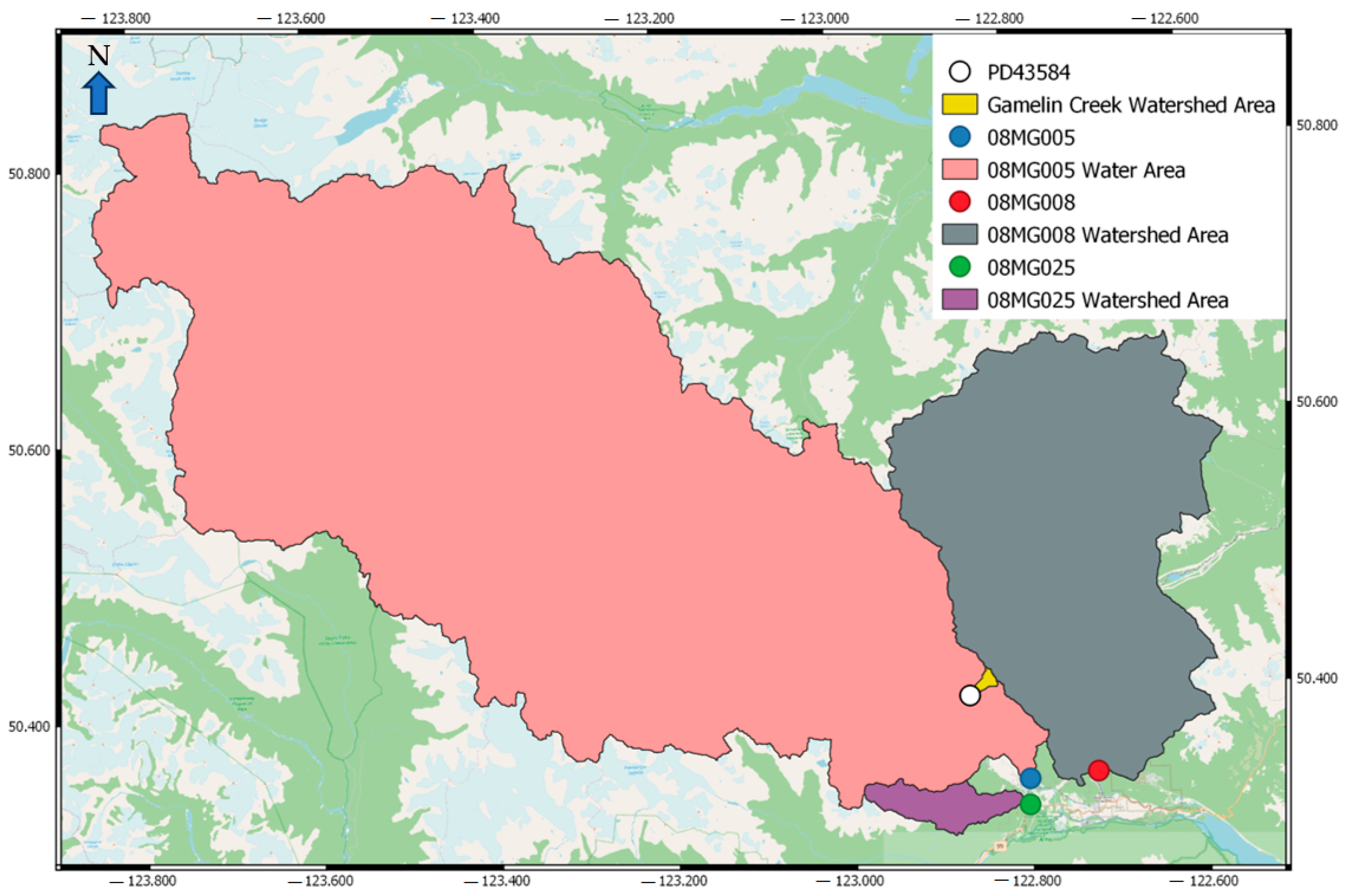
Using $DEMs$, we meticulously delineated the watershed boundaries for each gauged and $u_g$ watershed. The delineation process was carried out to accurately define the contributing areas and ensure consistency in the dataset. Below is the watershed delineation at the outlet for Gamelin Creek (represented by PD43584 in Figure 3), provided as an example in our analysis.

3.

Area, Elevation, and Slope Estimation

The $QGIS SAGA$ plugin was employed to calculate the watershed area, mean elevation, and mean slope for the $NNs$ of the $u_g$ watershed. This provided a quantitative basis for comparing the physical characteristics of the $u_g$ watershed with its neighboring watersheds.

• While watershed area and elevation are the primary factors used to identify $NNs$ and drive the streamflow prediction process, slope has also been incorporated due to its significant role in runoff generation, particularly in low-lying areas. As noted in the Introduction section, in regions where rainfall is the dominant driver of streamflow and elevation has minimal influence, slope becomes a crucial factor in determining streamflow magnitudes. This relationship has been well-documented in $BC$ by Sharma and Dery [22], reinforcing the importance of integrating slope alongside area and elevation to enhance the accuracy of hydrological modeling.

4.

Sorting by Elevation and Slope Difference

The $NNs$ were further sorted based on the absolute difference in mean elevation and slope between each $NN$ and the $u_g$ watershed. This secondary sorting step ensured that the watersheds with the most similar topographical characteristics were prioritized for subsequent analysis.

5.

Flow Data Extraction

Flow magnitude data for the selected $NNs$ were obtained from multiple sources to ensure a comprehensive hydrological assessment. These sources included: (1) the Water Survey of Canada’s database (https://wateroffice.ec.gc.ca/; accessed on 14 January 2025), (2) Surface Water-managed hydrometric stations, (3) municipal government records, and (4) public contributions. The dataset comprised mean monthly flow values, spot measurements, and observations of maximum and minimum flow occurrences, all of which were essential for characterizing the hydrological patterns of the selected $NNs$ and improving the reliability of streamflow predictions.

6.

Selection of NNs for Data Coverage

To ensure a comprehensive and accurate representation of flow data, the $NNs$ were chosen in a specific sequence. The process began by selecting the $NN$ with the smallest elevation or slope difference compared to the $u_g$ watershed. This was carried out to ensure that the first $NN$ was hydrologically similar, as elevation or slope can significantly influence streamflow. Once the first $NN$ was selected, additional $NNs$ were added one by one in iterative steps. The goal was to ensure that for each month of the year, there were at least two mean monthly flow values available from different $NNs$. This selection strategy was informed by observations during the cross-validation phase, where it became evident that the most accurate predictions occurred when each month was represented by flow data from at least two $NNs$. Using fewer than two $NNs$ often failed to capture the variability in flow patterns, resulting in oversimplified outputs. Conversely, incorporating more than two $NNs$ tended to introduce unnecessary complexity and led to overly smoothed predictions. These findings are consistent with prior studies by Samaniego et al. [24] and Qamar et al. [8], which also emphasized the importance of balancing representativeness and model parsimony in $NNs$ selection.

7.

Prediction of Flow Data for $u_g$ Watersheds

Once the $NNs$ were selected, each $NN$ in the cluster was alternately treated as $u_g$. For the remaining $NNs$ with known hydrological data, the flow data at the $u_g$ watershed was predicted using the proposed approach, broadly summed up in the following steps:

• The flow data (obtained from multiple sources mentioned above) for each watershed with known flow was normalized by dividing the monthly flow values by the watershed area, producing a unit area discharge value $\left({\displaystyle \raisebox{1ex}{$\raisebox{1ex}{${\mathrm{m}}^3$}\!\left/ \!\raisebox{-1ex}{$\mathrm{s}$}\right.$}\!\left/ \!\raisebox{-1ex}{${\mathrm{m}}^2$}\right.}\right)$.
• The normalized flow data were then scaled up to match the watershed area of the $u_g$ watershed, providing an initial prediction of the flow.
• To further refine the prediction, the scaled-up flow data were normalized based on the elevation and slope of each watershed, accounting for topographical influences.
• The adjusted flow values for each $NN$ were averaged, yielding a representative predictive monthly flow dataset (expressed as two column vectors) for the $u_g$ watershed. Watershed area, elevation, and slope were used as mathematical operators in this process.

8.

Validation Using Mean Absolute Error ($\delta$)

The predicted flow data were compared with observed flow data at the gauged stations to calculate $\delta$. This process was repeated iteratively, with each basin being removed once to simulate an $u_g$ scenario. The error metric, representing $\delta$ for each basin $k$, was calculated as follows:

$${\delta }_k={\displaystyle \frac{1}{n}}{\sum }_{i=1}^n\left|P_{ik}-O_{ik}\right|$$

(1)

where $P_{ik}$ and $O_{ik}$ are the predicted and observed flow values, respectively, and $n$ is the number of observations.

By systematically iterating through all basins, the methodology ensured robustness and consistency in the predictive flow estimates for $u_g$ watersheds.

Mathematically, the modeling process can be defined as the following steps.

Definitions:

$Q_u\left(m\right)=$ Predicted flow for the original $u_g$ watershed $u$ for month $m$.

$Q_i\left(m\right)=$ Measured flow for the gauged watershed $i$ for month $m$.

$n=$ Total number of gauged $NNs$ used for prediction.

$A_u, A_i=$ Watershed area of the $u_g$ and gauged watershed $i$, respectively.

$E_u, E_i=$ Mean elevation of the $u_g$ and gauged watershed $i$, respectively.

$S_u, S_i=$ Mean slope of the $u_g$ and gauged watershed $i$, respectively.

$w_i=$ Weight assigned to each gauged $NN$ (optional, default is equal weighting).

• Step 1: Normalizing Flows by Watershed Area

To normalize the monthly flow $Q_i\left(m\right)$ of each gauged station $i$ of the current month $m$ by its watershed area:

$$Q_i^{\prime }(m)={\displaystyle \frac{Q_i\left(m\right)}{A_i}}$$

(2)

• Step 2: Normalizing by Elevation and Slope

For each gauged station $i$, normalize the area-normalized flow $Q_i^{\prime }\left(m\right)$ using elevation and slope:

Elevation Normalization

$$Q_{i,E}^{\prime }(m)={\displaystyle \frac{Q_i^{\prime }\left(m\right)}{E_i}}={\displaystyle \frac{Q_i\left(m\right)}{A_i·E_i}}$$

(3)

Slope Normalization

$$Q_{i,S}^{\prime }(m)={\displaystyle \frac{Q_i^{\prime }\left(m\right)}{S_i}}={\displaystyle \frac{Q_i\left(m\right)}{A_i·S_i}}$$

(4)

• Step 3: Treating Each Gauged Station as ${\mathit{u}}_{\mathit{g}}$

Each $NN$ $i$ is treated as if it were ${u_g}^i$. Its flow is predicted using the remaining $NNs$ by scaling the normalized flows back (or up) to the characteristics of ${u_g}^i$.

• Predicting Flow for Each $NN$ using Area:

$$Q_{u,A}^{\left[i\right]}\left(m\right)=A_u^{\left[i\right]}·\left({\displaystyle \frac{1}{n-1}}{\sum }_{j\ne i}{Q}_{j,A}^{\prime }(m)\right)$$

(5)

where $j$ represents the remaining number of $NNs$ after $i$ is assumed to be $u_g$ and removed from the dataset.

• Predicting Flow for Each $NN$ using Elevation:

$$Q_{u,E\uparrow }^{\left[i\right]}\left(m\right)=A_u^{\left[i\right]}·E_u^{\left[i\right]}·\left({\displaystyle \frac{1}{n-1}}{\sum }_{j\ne i}{Q}_{j,E}^{\prime }(m)\right) \mathrm{and}$$

(6)

$$Q_{u,E\downarrow }^{\left[i\right]}\left(m\right)={\displaystyle \frac{A_u^{\left[i\right]}}{E_u^{\left[i\right]}}}· \left({\displaystyle \frac{1}{n-1}}{\sum }_{j\ne i}{Q}_{j,E}^{\prime }(m)\right)$$

The position of elevation in the denominator indicates that elevation is inversely proportional to watershed streamflow.

• Predicting Flow for Each $NN$ using Slope:

$$Q_{u,S}^{\left[i\right]}\left(m\right)=A_u^{\left[i\right]}·S_u^{\left[i\right]}·\left({\displaystyle \frac{1}{n-1}}{\sum }_{j\ne i}{Q}_{j,S}^{\prime }(m)\right)$$

(7)

• Step 4: Averaging Monthly Predictions

To obtain the final predicted flow for each $NN$ treated as ${u_g}^i$, we take the average of the predicted flows $\left(\overline{Q}\right)$ over all the months:

• Average Monthly Flow using Area:

$${\overline{Q}}_{u,A}^{\left[i\right]}={\displaystyle \frac{1}{12}}{\sum }_{m=1}^{12}{Q}_{u,A}^{\left[i\right]}\left(m\right)$$

(8)

• Average Monthly Flow using Elevation:

$${\overline{Q}}_{u,E}^{\left[i\right]}={\displaystyle \frac{1}{12}}{\sum }_{m=1}^{12}{Q}_{u,E}^{\left[i\right]}(m)$$

(9)

• Average Monthly Flow using Slope:

$${\overline{Q}}_{u,S}^{\left[i\right]}={\displaystyle \frac{1}{12}}{\sum }_{m=1}^{12}{Q}_{u,S}^{\left[i\right]}(m)$$

(10)

• Step 5: Calculating $\mathit{\delta }$

To determine which normalization (area, elevation, or slope) is more effective, compare the predicted flows with the actual flows using $\mathit{\delta }$:

• $\mathit{\delta }$ for Area:

$${\mathit{\delta }}_A={\displaystyle \frac{1}{n}}{\sum }_{i=1}^n\left|{\overline{Q}}_i-{\overline{Q}}_{u,A}^{\left[i\right]}\right|$$

(11)

• $\mathit{\delta }$ for Elevation:

$${\mathit{\delta }}_E={\displaystyle \frac{1}{n}}{\sum }_{i=1}^n\left|{\overline{Q}}_i-{\overline{Q}}_{u,E}^{\left[i\right]}\right|$$

(12)

• $\mathit{\delta }$ for Slope:

$${\mathit{\delta }}_S={\displaystyle \frac{1}{n}}{\sum }_{i=1}^n\left|{\overline{Q}}_i-{\overline{Q}}_{u,S}^{\left[i\right]}\right|$$

(13)

• Step 6: Predicting Flow for the Original ${\mathit{u}}_{\mathit{g}}$

Whichever normalization (elevation or slope) produces the lowest $\mathit{\delta }$ is selected for predicting the flows for the original $u_g$:

$$Q_u\left(m\right)=\left\{\begin{array}{c}{A}_u·\left({\displaystyle \frac{1}{n}}{\sum }_{i=1}^n{Q}_{i,E}^{\prime }\left(m\right)\right), if {\mathit{\delta }}_A<{{\mathit{\delta }}_{E\uparrow },\mathit{\delta }}_{E\downarrow },{\mathit{\delta }}_S\\ A_u·E_u\uparrow ·\left({\displaystyle \frac{1}{n}}{\sum }_{i=1}^n{Q}_{i,E}^{\prime }(m)\right), if {\mathit{\delta }}_{E\uparrow }<{{\mathit{\delta }}_A,{\mathit{\delta }}_{E\downarrow },\mathit{\delta }}_S \\ {\displaystyle \frac{A_u}{E_u\downarrow }}·\left({\displaystyle \frac{1}{n}}{\sum }_{i=1}^n{Q}_{i,E}^{\prime }(m)\right), if {\mathit{\delta }}_{E\downarrow }<{{\mathit{\delta }}_A,{\mathit{\delta }}_{E\uparrow },\mathit{\delta }}_S \\ A_u·S_u·\left({\displaystyle \frac{1}{n}}{\sum }_{i=1}^n{Q}_{i,S}^{\prime }(m)\right), if {\mathit{\delta }}_S<{{\mathit{\delta }}_A,{\mathit{\delta }}_{E\uparrow },\mathit{\delta }}_{E\downarrow }\end{array}\right.$$

(14)

Note that the downward arrows $(\downarrow )$ indicate stations where the inverse relationship between elevation and discharge was considered, as it resulted in a lower $\mathit{\delta }$ compared to the direct relationship $(\uparrow )$.

Final Predicted Flow for Each Month:

The final equation used to predict the monthly flow $Q_u\left(m\right)$ for the original $u_g$ is as follows:

$$Q_u\left(m\right)=P_u·A_u·\left({\displaystyle \frac{1}{n}}{\sum }_{i=1}^n{\displaystyle \frac{Q_i\left(m\right)}{A_i·P_i}}\right)$$

(15)

where $P$ is the chosen parameter (either area, elevation, or slope) based on which one resulted in the lower $\mathit{\delta }$. Please note that if the selected $P_u$ is elevation and is inversely related to discharge, then Equation (15) will be displayed as follows:

$$Q_u\left(m\right)={\displaystyle \frac{A_u}{P_u}}·\left({\displaystyle \frac{1}{n}}{\sum }_{i=1}^n{\displaystyle \frac{Q_i\left(m\right)}{A_i·P_i}}\right)$$

(16)

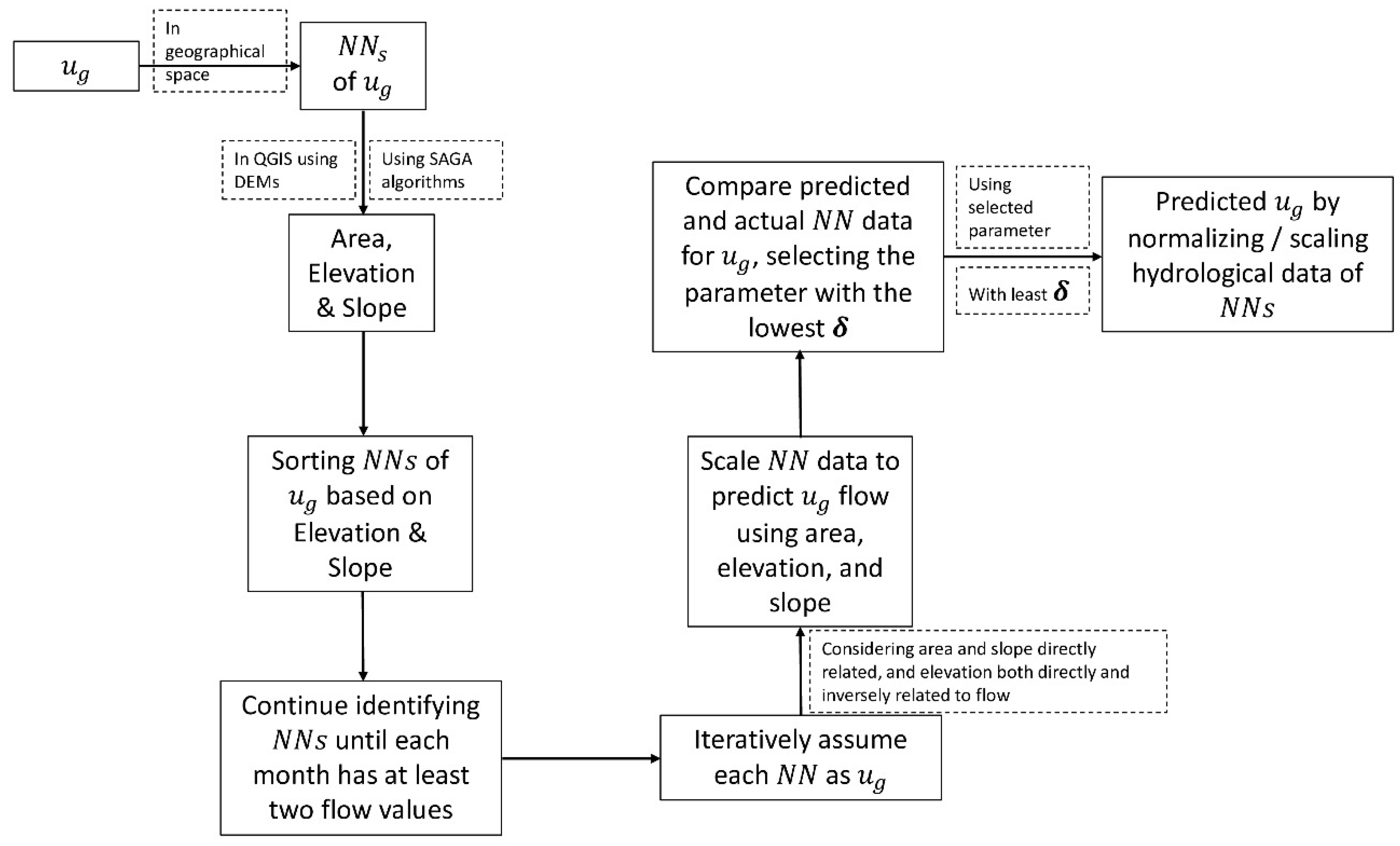
For improved clarity and understanding, the methodology is presented in Figure 4.

It is important to note that the hydrological zones delineated in Figure 2—based on the study conducted by Ahmed [19]—represent regions where watersheds exhibit strong correlations in flow behavior. Consequently, $NNs$ are selected exclusively from within these zones, ensuring consistency in flow-generating mechanisms between $u_g$ watershed and its neighbors.

4. Results and Discussion

To assess the effectiveness of the proposed methodology, we compiled observed streamflow data from various hydrometric stations managed by provincial hydrometric specialists, municipal governments, and observation stations. In cases where direct discharge measurements were not feasible, local residents recorded the months of maximum and minimum flow. The observed data were then compared with the predicted values. As detailed in previous sections, some hydrometric stations recorded data at high temporal resolutions, including 15-minute intervals or daily measurements. To standardize the dataset for analysis, these high-resolution observations were aggregated to a monthly time scale by computing the mean discharge for each month using $R$ (version 4.3.0).

The watersheds analyzed in this study are primarily influenced by rainfall in the southern regions of the province and by snowmelt in the northern regions of British Columbia. To evaluate the performance of the proposed methodology, we compared the results with the conventional $DAR$ method, which serves as a key normalization parameter alongside elevation and slope. In regions lacking installed hydrometric gauges, supplementary information was obtained from residents whose families have lived in the area for multiple generations. These individuals, who either utilize water from nearby channels or possess extensive knowledge of regional flow patterns, provided qualitative insights into seasonal discharge variability.

As outlined in the Methodology section, while the relationship between watershed slope and discharge is direct, the connection between elevation and discharge is less certain. To assess the relationship between elevation and discharge, we calculated the $\mathit{\delta }$ in the $NNs$ of $u_g$ under two assumptions: one where elevation is directly related to discharge, and another where this relationship is not assumed. This process was repeated for all $NNs$, with the predicted monthly streamflows compared to the observed streamflows for each $NN$. The relationship that resulted in the lowest $\mathit{\delta }$ was selected for predicting the hydrological data at $u_g$.

Table 2. $\mathit{\delta }$ values for streamflow prediction in the NNs of $u_g$ using area, elevation, and slope as normalization parameters. Bold values indicate the selected parameter for each station, as it yielded the lowest $\mathit{\delta }$ compared to the others.

Station	Area	Elevation	Slope
08MH082	0.053	0.111	0.053
08MH098	0.021	$0.029 (\downarrow )$	0.071
08MH0051	0.136	0.169	0.400
PD200737	1.466	4.418	2.825
08MH084	0.066	0.005	0.150
08MH152	0.113	0.079 $(\downarrow )$	0.101
08MH156	0.149	0.120 $(\downarrow )$	0.126
08MH153	0.058	0.049 $(\downarrow )$	0.115
08MH055	0.447	0.372 $(\downarrow )$	1.154
08MH0058	0.126	0.097	0.174
08MH0055	0.162	0.075	0.114
HYD-GIBS-R1	0.593	0.564	0.790
PD189470	0.541	0.151	0.215
PD43584	40.551	38.381	40.991
08MH157	6.523	2.303	1.322
08MH104	0.227	0.251	0.063
08MH155	0.207	0.216	0.035
08MH0041	0.280	0.447	0.270
08MH0004	12.086	11.120	8.198

displays the $\mathit{\delta }$ values obtained by utilizing area, elevation, and slope as normalization parameters for streamflow prediction in the $NNs$ of $u_g$.

Notably, stations such as 08MH098, 08MH152, 08MH156, 08MH153, and 08MH055 demonstrated improved prediction accuracy when the inverse relationship between elevation and discharge was applied. In contrast, for other stations, the direct relationship between elevation and discharge, or the use of other normalization parameters, yielded the most accurate results. These variations emphasize the significance of considering alternative relationships for elevation as a normalization parameter, underscoring the need for a flexible approach when optimizing streamflow predictions in the current modeling framework.

The relationship between elevation and streamflow varies across the study area. While most of the stations in the study area exhibit a direct relationship with mean elevation, some stations show an inverse relationship between elevation and flow. This pattern is particularly evident in larger watersheds, such as 08MH055. This inverse trend in higher-elevation watersheds is likely influenced by a combination of delayed snowmelt contributions, high infiltration rates—suggested by Google Earth imagery indicating dense vegetation—longer water travel times (time of concentration), and precipitation distribution patterns. Identifying the dominant factor requires further analysis of precipitation data, land cover, soil permeability, and groundwater interactions.

Similarly, the inverse relationship between elevation and flow in lower-elevation watersheds along the international border between the USA and Canada (08MH152, 08MH153, and 08MH156) can be attributed to increasing groundwater contributions as the point of interest within the watershed shifts downstream. Groundwater contributions were particularly evident during our field visits, and an image from one of these visits is provided below in Figure 5:

Notably, 08MH098 is located on West Creek, near its drainage point into the Fraser River, making it more susceptible to groundwater influence.

We observed that for $u_g$ watersheds, better predictive results were achieved when the $NNs$ had similar watershed characteristics to those of the $u_g$. The normalization procedure tended to produce less efficient results when it was applied to watersheds with significant differences in characteristics. In contrast, when the $u_g$ and its $NNs$ had similar characteristics, less normalization was required, leading to more accurate predictions. For instance, watershed PD43584 had a $\mathit{\delta }$ of 38.381—significantly higher than that of other watersheds in the study, such as 08MH082. This can be explained by the substantial variation in size among PD43584’s NNs, which leads to significant differences in discharge magnitudes. In particular, one of its NNs, 08MG005, exhibits a much higher discharge than the others, which skews the normalization and results in a disproportionately high $\mathit{\delta }$ value. As a result, predictive performance at 08MH082 is theoretically expected to be more reliable than at PD43584, given its more consistent watershed characteristics.

Table 3. Minimum, average, and maximum variations in characteristics between the $u_g$ and $NNs$ and the corresponding $\eta$ and $\mathit{\delta }$ values. “NA” in the table refers to an observation post for which monthly quantitative data were not available.

Hydrometric Station	$\mathbf{Area} \mathbf{\left(}{\mathbf{m}}^2\mathbf{\right)}$	Parameter Used	$\mathbf{Variation} \mathbf{(}\mathbf{\%}\mathbf{)} \mathbf{of} \mathbf{Watershed} \mathbf{Characteristics} \mathbf{(}\mathbf{Between} {\mathit{u}}_{\mathit{g}}$$\mathbf{and} \mathbf{its} {\mathit{N}\mathit{N}}_{\mathit{s}}\mathbf{)}$			Performance Parameters
			Minimum Variation	Average Variation	Maximum Variation	$\mathit{\eta }$	$\mathit{\delta }$
08MH0058	1,691,188	Elevation	4.476	11.614	20.818	0.854	0.016
08MF0004	12,056,212	Elevation	3.870	79.514	155.158	0.247	0.276
08MH0051	14,836,529	Elevation	0.507	15.236	33.827	0.377	0.284
08MH084	28,149,549	Elevation	4.686	9.034	20.638	0.950	0.143
08MH0055	5,056,045	Elevation	11.464	18.463	27.951	0.816	0.0283
08MH157	39,879,899	Elevation	18.791	18.791	18.791	−1.908	2.070
08MH055	426,331,622	Elevation	18.791	18.791	18.791	−1.405	20.577
HYD-GIBS-R1	3,337,955	Elevation	0.404	24.118	78.122	0.160	0.041
PD189470	1,230,405	Elevation	81.420	84.930	88.440	−0.707	0.044
PD43584	2,495,115	Elevation	24.165	28.015	32.628	NA	NA
08MH082	11,975,962	Area	5.606	9.033	12.126	0.597	0.139
08MH098	12,900,703	Area	5.606	9.033	12.126	0.975	0.041
08MH156	15,069,903	Area	5.269	21.902	38.534	0.657	0.117
08MH0041	26,822,502	Slope	17.396	18.166	18.937	0.910	0.142
08MH153	20,636,495	Slope	5.269	21.902	38.534	0.866	0.191
08MH152	35,091,991	Slope	5.269	21.902	38.534	0.415	0.294
08MH104	26,357,626	Slope	1.901	1.901	1.901	0.843	0.145
08MH155	70,330,390	Slope	1.901	1.901	1.901	0.789	0.395
PD200737	7,569,104	Slope	1.961	158.157	325.013	0.0746	0.095

presents $\mathit{\delta }$ and Nash–Sutcliffe efficiency values for various watersheds, calculated using the hydroGOF package in R(version 4.3.0) [25], highlighting how these metrics vary based on differences in watershed characteristics between $u_g$ and its $NNs$. The table also identifies the normalization parameter selected for each station and demonstrates how $\mathit{\delta }$ and $\eta$ change depending on the degree of variation—both minimum and maximum—in watershed characteristics between $u_g$ and its $NNs$.

The minimum, average, and maximum variations in watershed characteristics between the target watershed $\left(u_g\right)$ and its $NNs$, along with the corresponding performance parameters, $\eta$ and $\delta$ in Table 3, highlight how different hydrometric stations exhibit varying degrees of similarity to $u_g$ in terms of elevation, watershed area, and slope. The variation percentages indicate the extent of deviation of each $NN$ from $u_g$, with lower values representing greater similarity.

For stations where elevation was used as the primary normalization parameter, the variation ranged from as low as 0.404% (HYD-GIBS-R1) to as high as 88.44% (PD189470). Notably, larger deviations in elevation were associated with lower $\eta$ values, suggesting reduced predictive performance, as seen in PD189470 ($\eta$ = −0.707). Conversely, stations with relatively low variation, such as 08MH084 (average variation = 9.034%), exhibited higher performance with $\eta$ values approaching 1.

Similarly, when the watershed area was used as the normalization parameter, variations remained moderate, with maximum deviations around 38.534% (08MH082, 08MH098, and 08MH156). In these cases, the $\eta$ values generally remained positive, indicating reasonable predictive accuracy.

For stations where slope was the chosen parameter, variation patterns varied widely. While some stations (e.g., 08MH104 and 08MH155) showed minimal variation (1.901%), others, such as PD200737, exhibited extreme deviations, exceeding 300%. Interestingly, extreme variations in slope were associated with significantly lower $\eta$ values (e.g., $\eta$ = 0.0746 for PD200737), highlighting the critical importance of selecting $NNs$ with watershed characteristics that closely match those of $u_g$ to ensure more reliable predictions.

Overall, the table underscores that $\eta$ and $\delta$ values are sensitive to the choice of normalization parameter and the degree of variation between $u_g$ and its $NNs$. The findings suggest that selecting the most appropriate $NNs$ for $u_g$ should be guided by minimizing the variation between $NNs$ and $u_g$. Moreover, by reviewing Table 3 and

Table 4. Predicted vs. actual flows of Wilfred Creek with and without spring contribution.

Month	Flow of Creek (Including Spring Contribution)	Predicted Flows	Spring Overflows	Revised Predicted Flows (Predicted Flows + Spring Overflows)
	${(\mathbf{m}}^3/\mathbf{s})$	${(\mathbf{m}}^3/\mathbf{s})$	${(\mathbf{m}}^3/\mathbf{s})$	${(\mathbf{m}}^3/\mathbf{s})$
January	0.101	0.0358	0.056	0.0918
February	0.201	0.0279	0.081	0.1089
March	0.180	0.0239	0.117	0.1409
April	0.164	0.0330	0.096	0.129
May	0.121	0.0597	0.066	0.1257
June	0.100	0.0575	0.055	0.1125
July	0.132	0.0292	0.062	0.0912
August	0.098	0.0124	0.043	0.0554
September	0.150	0.0090	0.039	0.048
October	0.091	0.0187	0.028	0.0467
November	0.065	0.0304	0.035	0.0654
December	0.074	0.0326	0.032	0.0646
Average	0.123	0.031	0.059	0.090

concurrently, it can be clearly interpreted that as the performance of the normalization parameter in predicting the hydrological data of $NNs$ deteriorates (resulting in larger $MAE$ values), the prediction performance for $u_g$ also declines. This indicates that the prediction performance can be assessed prior to the actual application of the model for $u_g$. For example, for hydrometric stations 08MH157, 08MH0004, and PD43584, the performance deteriorates, as shown in Table 3, with increasing $\delta$ values for predicting the hydrological data of $NNs$ for $u_g$. By the same token, stations 08MH098, 08MH084, and 08MH0058 demonstrated strong statistical performance, as reflected in their comparatively better predictive performance for predicting the hydrological data of their $NNs$, as shown in Table 2.

The results presented below illustrate the outcomes when the area parameter is utilized as the normalization parameter in the prediction process for $u_g$, where the area parameter yielded the least error among the $NNs$ for these stations.

Figure 6 compares observed (“Actual”) and modeled (“DAR”) streamflow discharge across four hydrometric stations, revealing seasonal variations in discharge trends. At station 08MH0051, the model underestimates discharge during the high-flow season (January to March) but aligns more closely during the low-flow period (May to September). Similarly, at 08MH082, the DAR model captures seasonal trends but overestimates discharge in the high-flow period, while providing a good fit during low-flow periods. Station 08MH098 exhibits strong agreement between modeled and observed values, with minimal deviations. At PD200737, the model underestimates streamflow during the summer months but aligns better in other periods. Overall, while the DAR method effectively captures seasonal discharge patterns, some discrepancies persist, particularly in high-flow conditions, indicating the need for further model refinement.

Building upon the analysis of the area normalization parameter, the subsequent results investigate the performance of the elevation parameter in normalizing the prediction of $u_g$.

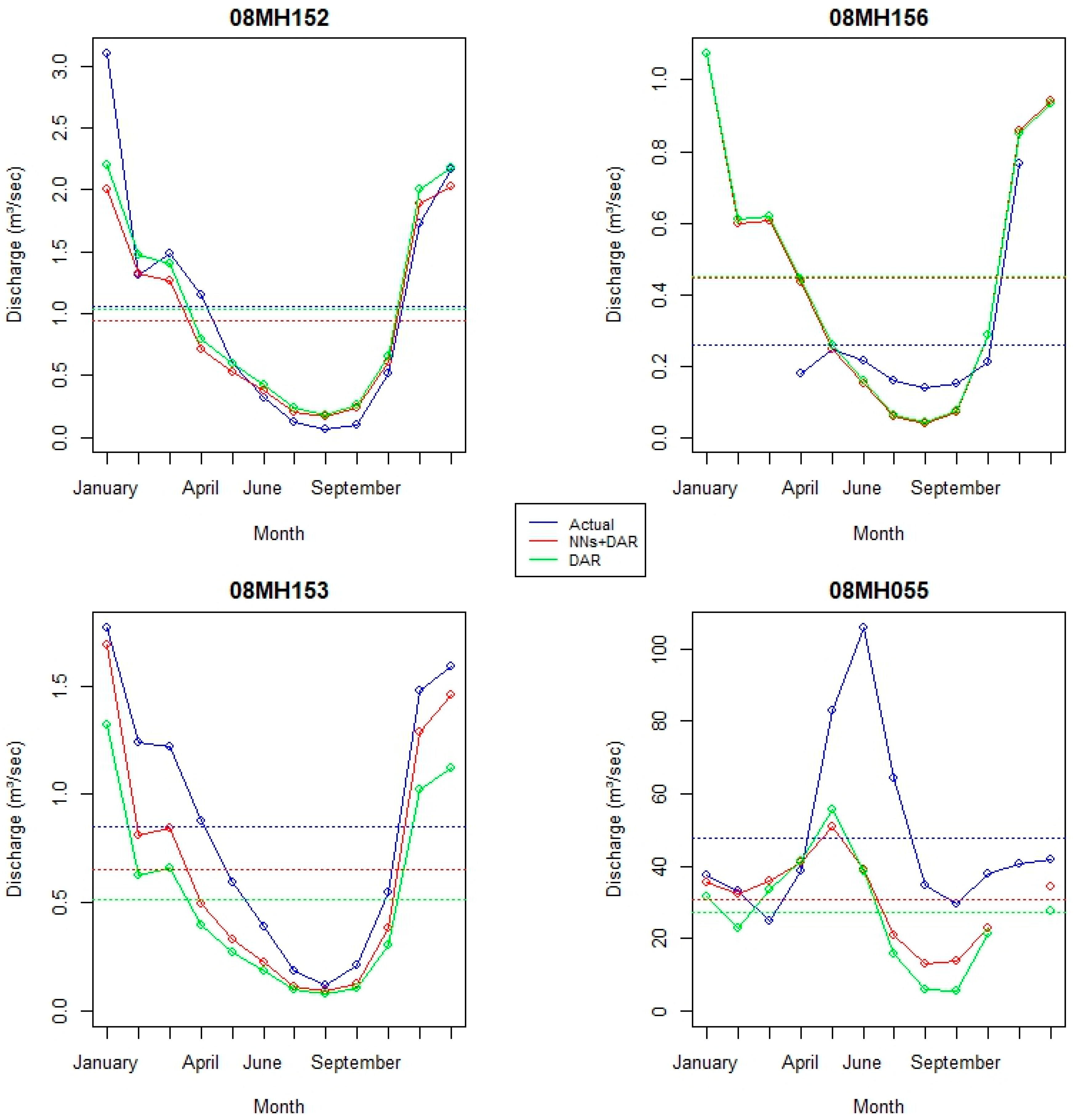
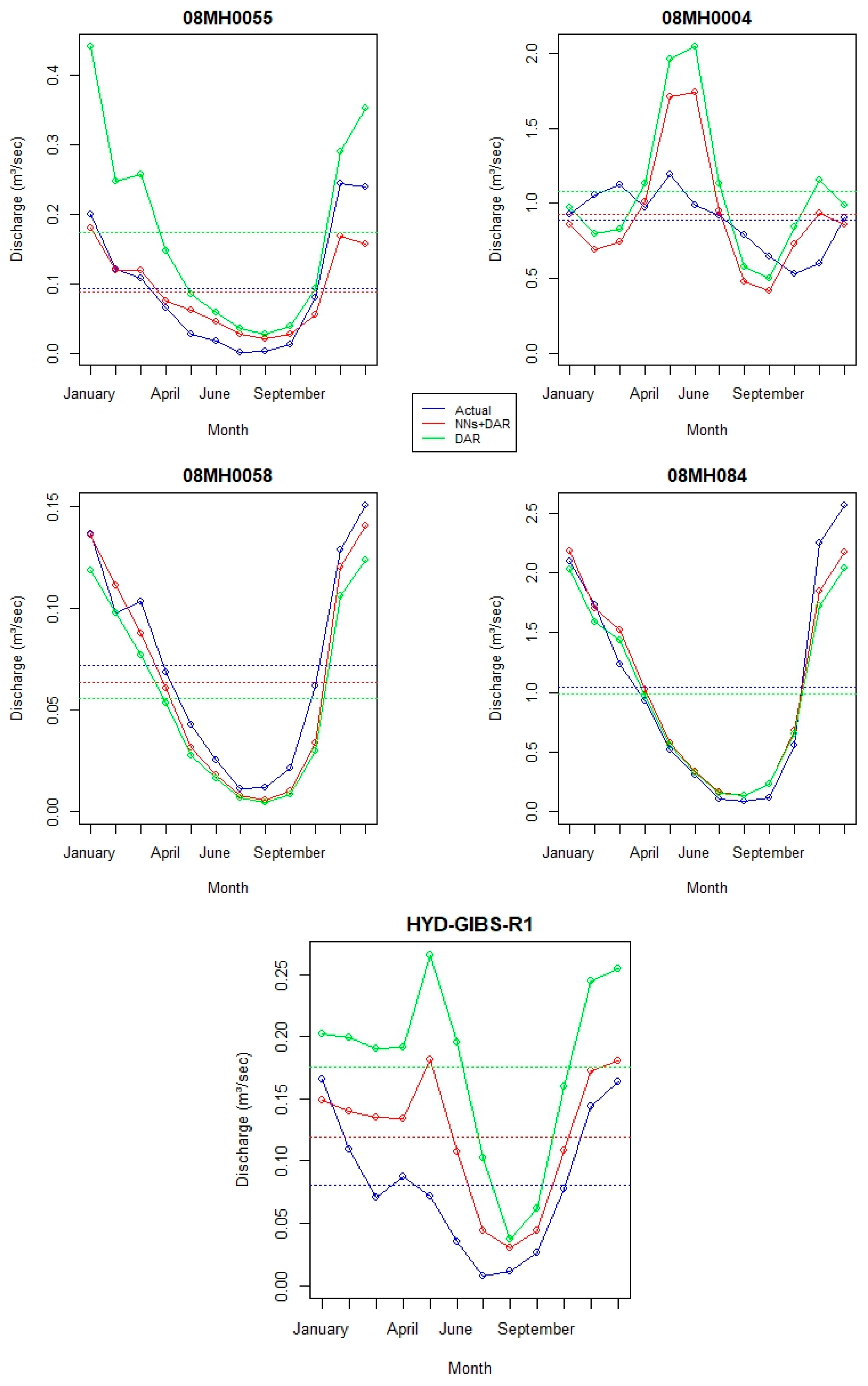
Figure 7 presents a comparison between predicted and observed discharge values across eight hydrometric stations: 08MH152, 08MH156, 08MH153, 08MH055, 08MH0055, 08MH0004, 08MH0058, and 08MH084.

For station 08MH152, observed discharge values (represented by the blue line) generally exceed predicted values during the high-flow period (January to March). However, during the low-flow period (June to August), predictions from both methods align more closely with the observed data. In station 08MH156, predictions from both the $NNs+DAR$ and $DAR$ methods are nearly identical, indicating that the inclusion of $NNs$ does not significantly enhance the accuracy over the $DAR$ method alone. Both methods, however, tend to underestimate discharge during the high-flow period.

For station 08MH153, the $NNs+DAR$ method provides improved prediction accuracy compared to $DAR$ alone, particularly during the high-flow period. Despite this improvement, both methods underestimate discharge during the low-flow period.

Station 08MH055 exhibits high variability in observed discharge values, with a notable peak in June. Neither prediction method successfully captures this sharp peak, although both methods adequately represent the overall seasonal trend. The $NNs+DAR$ method provides a better fit to observed discharge values than the $DAR$ method alone.

In station 08MH0055, both methods tend to underestimate discharge during high-flow periods (January to April) and overestimate during low-flow periods (July to August). However, the $NNs+DAR$ method provides a closer match to observed values compared to $DAR$ alone.

For station 08MH0004, observed discharge displays a significant peak in June, which is overestimated by the $DAR$ method, but more accurately captured by the $NNs+DAR$ approach. Both methods, however, tend to underestimate discharge during the winter months.

For station 08MH0058, both $NNs+DAR$ and $DAR$ methods closely track the observed discharge throughout the year, with slight underestimation during peak flows in January and overestimation during the late fall. These minor discrepancies indicate good predictive performance at this station. In station 08MH084, the observed, $NNs+DAR$, and $DAR$ lines are well-aligned, effectively capturing both high- and low-flow periods, suggesting that both methods perform similarly and effectively.

For HYD-GIBS-R1, the $DAR$ model tends to overestimate discharge, particularly during peak flow periods, indicating potential limitations in accurately capturing seasonal variability. In contrast, the $NNs+DAR$ hybrid method provides a closer approximation to actual discharge values, suggesting improved predictive capability. Notably, during the low-flow period around June, both models struggle to capture the sharp decline, though $NNs+DAR$ follows the trend more closely.

In general, the $NNs+DAR$ method generally improves prediction accuracy compared to the $DAR$ method alone, particularly in capturing seasonal trends and reducing errors during low-flow periods. However, challenges persist in accurately capturing sharp peaks and high-flow events, particularly at stations with more variable hydrological regimes, which may necessitate the introduction of basin-scale information into the current modeling framework.

Subsequent to the analysis of the elevation normalization parameter, the following section assesses the influence of the slope parameter on the normalization of $u_g$ predictions.

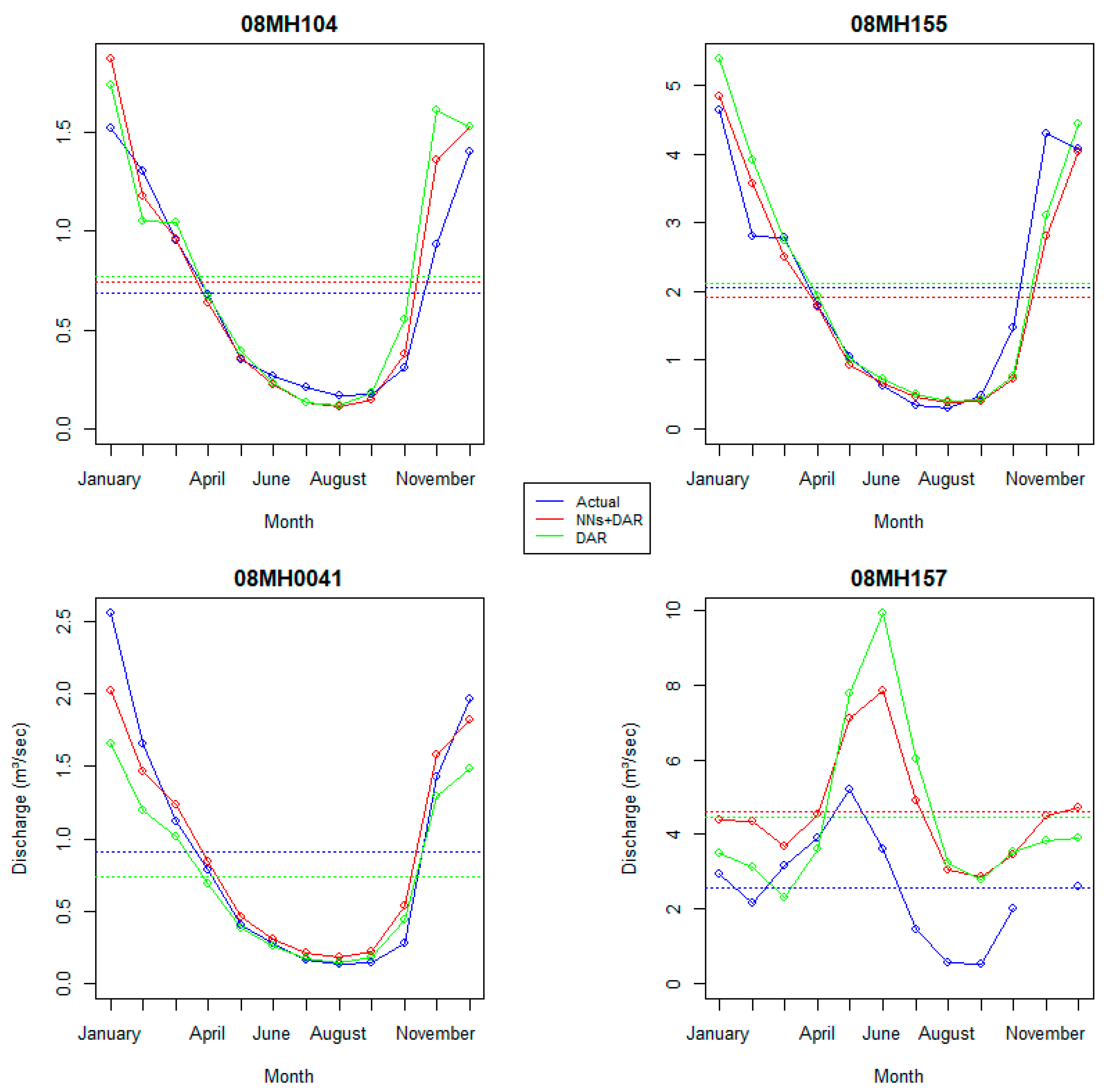
Figure 8 presents a comparison between predicted and observed discharge values for four hydrometric stations (08MH104, 08MH155, 08MH0041, and 08MH157), with the slope parameter used as the normalization parameter.

For station 08MH104, both prediction methods follow the seasonal trend of the actual data, although $DAR$ tends to slightly overestimate discharge in January and underestimate it during the late fall. The $NNs+DAR$ method provides a closer fit to observed data, especially during low-flow periods.

At station 08MH155, both the $NNs+DAR$ and $DAR$ methods show good agreement with actual discharge, effectively capturing both high- and low-flow periods, though $DAR$ slightly overestimates discharge in the winter months.

For station 08MH0041, both prediction methods underestimate peak flows observed in January and February but align well with actual values during the low-flow period (June to August). The $NNs+DAR$ approach provides a closer match to observed discharge throughout the year compared to $DAR$ alone.

In contrast, station 08MH157 exhibits higher variability in actual discharge, with a sharp peak observed around June. Both $DAR$ and $NNs+DAR$ methods overestimate flows during this period, although $NNs+DAR$ performs slightly better in aligning with the actual pattern. Additionally, both methods tend to overestimate discharge in the early months and underperform during the low-flow season.

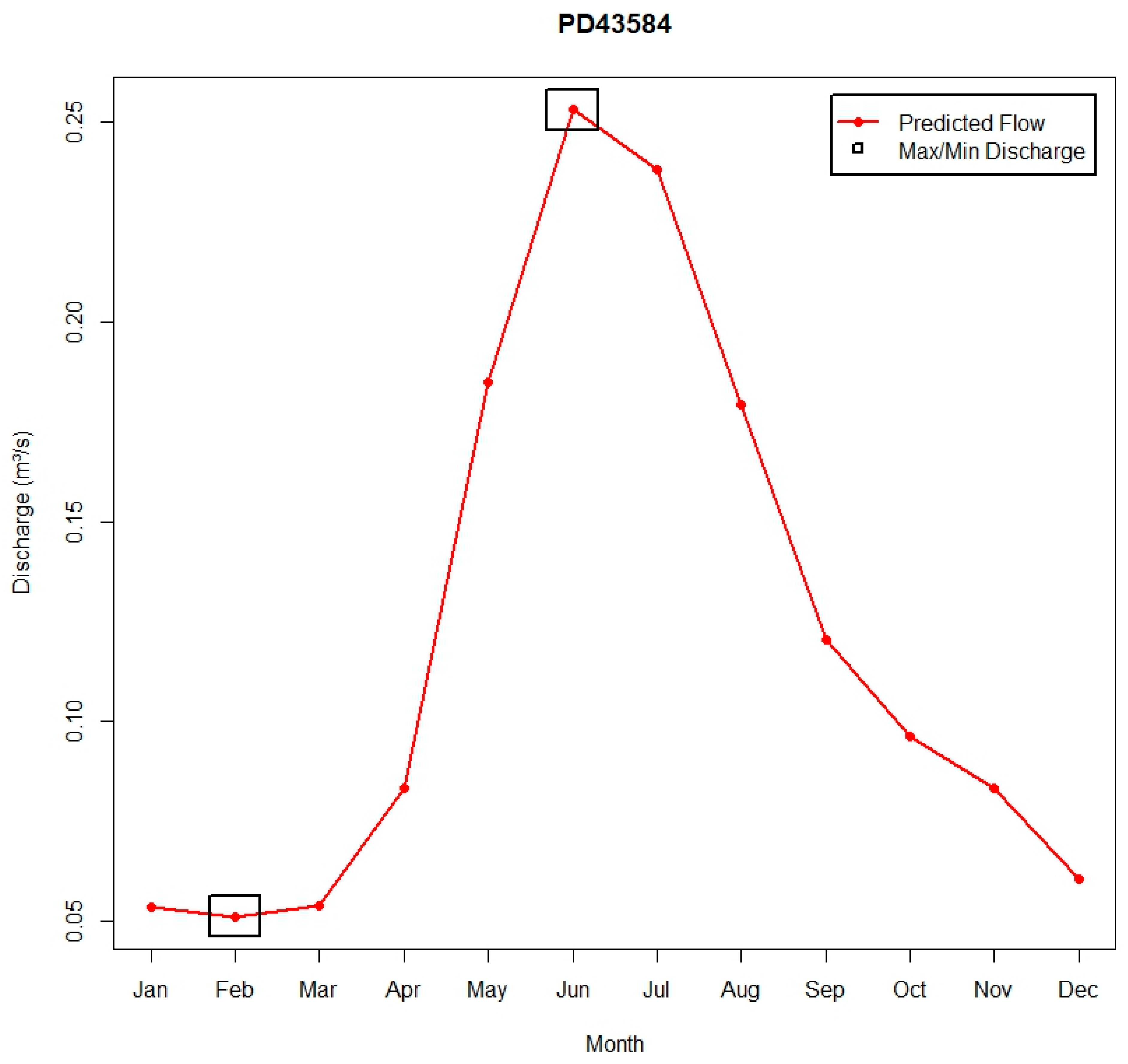
The above results also confirm that the proposed methodology consistently predicts the months of maximum and minimum monthly flow. This accuracy was further validated for PD43584, designated as an “Observation Post,” where local Indigenous knowledge was employed to determine the timing of peak and lowest flow values. The predicted flow rates and their corresponding months are presented in Figure 9.

For PD43584, the observed maximum monthly flow occurs in June, while the minimum flow is recorded during the winter months, aligning precisely with the insights provided by local Indigenous knowledge.

An overall performance comparison of the proposed methodology with $DAR$ showed that the proposed methodology can predict hydrological data in $u_g$ watersheds with reasonable accuracy, making it applicable for predicting hydrological data elsewhere. Applying this methodology to $NNs$ of $u_g$ watersheds demonstrate their effectiveness at the local scale before extending their application to other $u_g$ watersheds. This property helps determine whether to use the methodology for predicting hydrological data for a specific point of diversion or to rely on information from another source if better results are not achieved in the $NNs$.

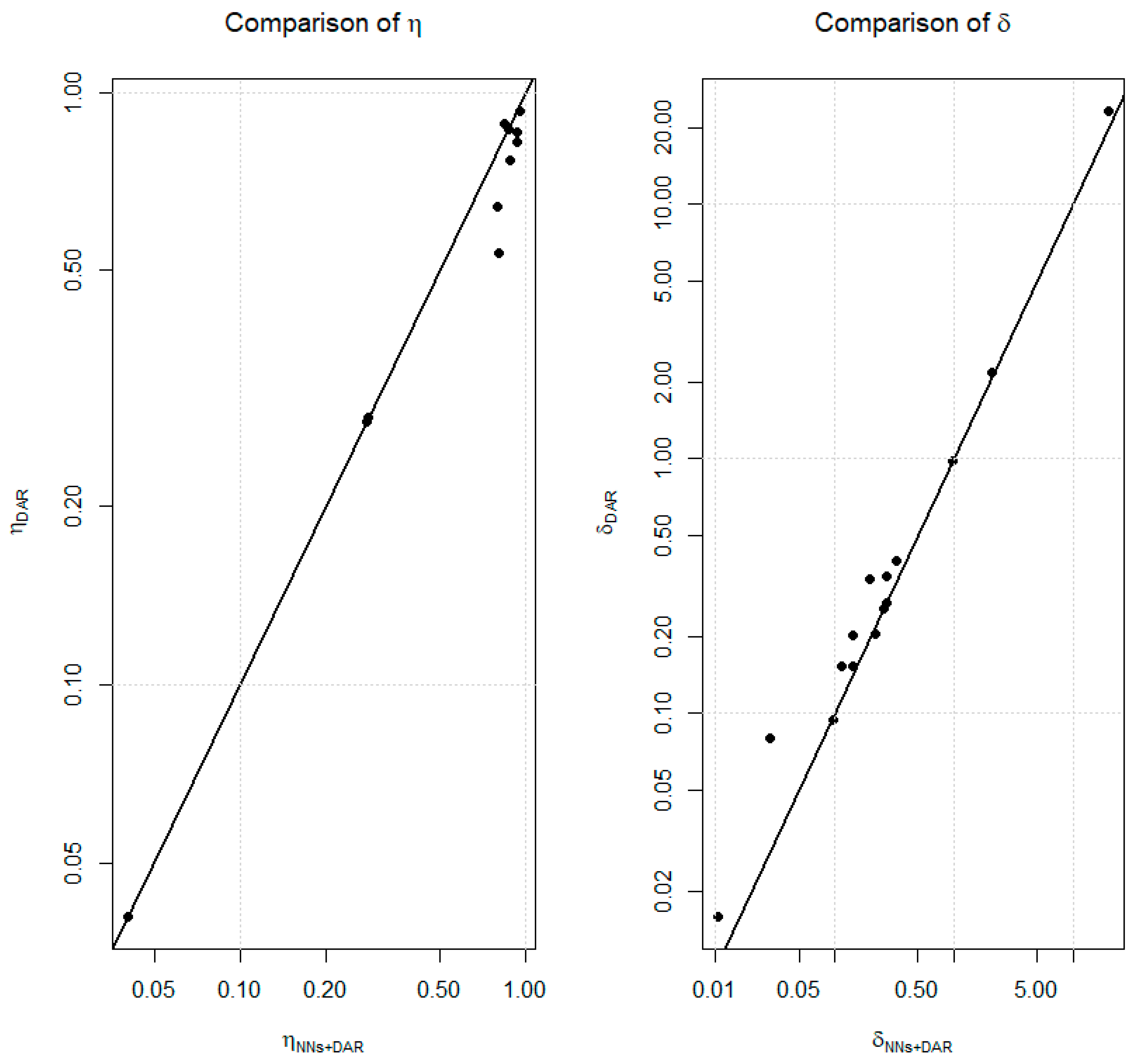
A comparative analysis of model performance for streamflow prediction using two methods: the $DAR$ method and $NNs+DAR$ approach are presented in the following Figure 10.

From the figure, it is clear that the $NNs+DAR$ method consistently outperforms the $DAR$ method alone in terms of both efficiency and accuracy across most hydrometric stations. Specifically, the $NNs+DAR$ approach yields higher efficiency values, indicating a better ability to reproduce the observed discharge variability and lower error, reflecting smaller deviations from actual streamflow data. The improvement is especially notable in stations with more complex and fluctuating flow regimes, where the combined method demonstrates significantly better performance with higher efficiency and reduced error. However, for stations characterized by stable and less variable streamflow patterns, both methods perform comparably, suggesting that the simpler $DAR$ method may still be sufficient in such cases. Overall, the figure underscores the effectiveness of integrating $NNs$ with $DAR$ for enhancing streamflow prediction accuracy, particularly in dynamically varying hydrological conditions where traditional methods may fall short.

Figure 6, Figure 7 and Figure 8 indicate that the model performs poorly for watersheds 08MH055 and 08MH157. This poor performance can be attributed to the transboundary nature of these watersheds—portions of their drainage areas extend into the United States. The DEMs used in our analysis are limited to the Canadian side of the international border and therefore only generate streamflow networks within Canadian territory. As a result, the delineation of these watersheds is incomplete (see Figure 11 below), leading to partial streamflow networks. This incomplete representation introduces inaccuracies in key watershed characteristics, including area, slope, and elevation, which, in turn, negatively impact the model’s predictive performance.

As illustrated in Figure 11 above, the delineation only covers the northern portion of the watersheds within Canada, with no contribution from the U.S. side.

Additionally, the performance deterioration is more pronounced for stations with larger watershed areas. For example, stations like 08MH157 and 08MH055, with watershed areas of 39,879,899 m² and 426,331,622 m², respectively, show much worse performance than stations with smaller areas, such as 08MH0058 (1,691,188 m²) or 08MH104 (26,357,626 m²). Larger watersheds tend to exhibit more complex and varied hydrological behavior, making it more difficult for the model to accurately predict flow dynamics when there is significant variation in watershed characteristics. This highlights the importance of both the similarity in characteristics between the station and its $NNs$ and the size of the watershed in determining the model’s predictive accuracy.

This issue becomes particularly pertinent when the $NN$ of an $u_g$ is a substantially larger water body, such as a major river, compared to the other $NNs$. It also arises when predicting flow for a tributary watershed using data from a much larger hydrological system. To address such cases, we propose either excluding watersheds with significant area discrepancies or, if exclusion is not feasible, incorporating additional neighboring watershed(s) to normalize the impact of including a significantly larger water body. While establishing what constitutes a “significantly larger” watershed can be complex, this methodology proves valuable when it is necessary to incorporate a hydrologically distinct or larger watershed into the analysis in order to ensure comprehensive data coverage across all twelve months of the year. This approach is particularly useful when a suitable $NN$ cannot be identified, necessitating the selection of a more compromise-prone $NN$.

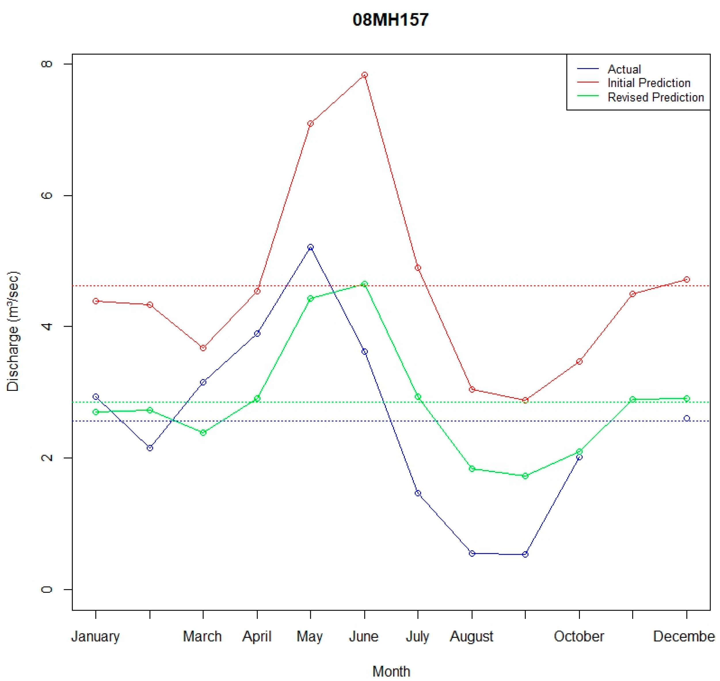
A practical example of this approach is demonstrated in the flow prediction for station 08MH157, where the $NNs$ 08MH004 and 08MH055 were selected due to their minimal $\delta$ in relation to the normalization parameter of elevation (see Figure 12 below). To mitigate the risk of oversimplifying the results, the larger watershed 08MH055 was chosen despite its considerable size and elevation. To balance the impact of including a large watershed (with a portion of its area located in the United States and, therefore, not fully delineated in the stream network), we also incorporated watershed 08MH163—entirely located within Canada and covering an area of 26,075,739 m²—as an additional neighboring watershed in the analysis. This adjustment helped correct the oversimplification introduced by the inclusion of a hydrologically dominant watershed.

Figure 12 above demonstrates the marked improvement in prediction accuracy achieved by applying the scaling factors derived from this procedure. Specifically, the performance indicators were enhanced, with $\delta$ reducing from 2.070 to 0.794 and $\eta$ increasing from −1.908 to 0.520. The dotted lines represent the mean monthly discharge for each dataset: actual, initial prediction, and revised prediction. The placement of these mean values highlights the tendency of the initial prediction to overestimate discharge, while the revised prediction more closely approximates observed trends. These results demonstrate the effectiveness of incorporating additional $NNs$ to improve streamflow predictions, particularly when dealing with larger watersheds that extend beyond Canada’s borders and, therefore, lack complete delineation. This approach contributes to a more robust and reliable modeling framework.

The accuracy of predicted discharge data can be significantly affected by anthropogenic activities as well, particularly during critically low-flow periods and peak irrigation demand months, as unauthorized water diversions across British Columbia’s water channels contribute to flow variability and discrepancies between observed and predicted values [26]. These diversions disrupt the natural flow regime by introducing artificial and undocumented alterations, especially in upstream areas. When diversions occur upstream of gauging stations, they reduce recorded flow volumes, which are crucial for model calibration and validation. As a result, prediction models misinterpret these diminished flows as indicative of natural conditions, leading to a systematic underestimation of streamflow in downstream and $u_g$ regions. This issue is particularly relevant in cases where a disproportionate amount of unauthorized water is diverted from a stream surrounded by agricultural areas, compared to its $NNs$ with minimal agricultural influence. Here, we must note that an argument can be made that the presence of unauthorized water diversions (i.e., the extraction or redirection of water without a valid license or in excess of permitted amounts) in historical records means they are inherently included in the observed discharge data used for model training. However, the critical issue is the interannual variability of these unauthorized diversions, which introduces uncertainty in the prediction process. The proposed models are trained on past data that reflect a mixture of natural flows and any historical anthropogenic alterations, including unauthorized diversions. While this enables the model to implicitly learn patterns under past diversion conditions, it does not account for year-to-year fluctuations in the magnitude, timing, or spatial distribution of unauthorized diversions, particularly during periods of low flow and high irrigation demand. These variations are unrecorded and differ significantly across watersheds depending on land use (e.g., intensity of agriculture), enforcement practices, and climatic conditions. Because there is no consistent or quantifiable record of unauthorized water use across the province, these diversions introduce a non-stationary component in the discharge data that the model cannot reliably capture or forecast. This contributes to the observed discrepancies between predicted and actual flows during critical periods.

Unauthorized diversions also undermine fundamental hydrological assumptions in predictive models, such as the assumed stability between watershed characteristics (e.g., area, slope, and elevation) and streamflow. These models are built on the premise of natural, unaltered systems; however, diversions artificially reduce flow magnitudes, weakening the model’s ability to make accurate predictions. The impacts of these diversions extend across watersheds, introducing errors that propagate through the network, distorting predictions for $u_g$ locations. This issue becomes particularly pronounced during extreme hydrological events such as drought, where unauthorized diversions can exacerbate low-flow conditions during droughts, further undermining prediction reliability. The lack of regulation and documentation of unauthorized diversions complicates efforts to quantify their impact, exacerbating underestimation and reducing the overall accuracy of streamflow models. To enhance future predictive models, we recommend incorporating the proportion of agriculturally licensed water use areas relative to the total agricultural or water consumption area, ensuring a more comprehensive representation of human-induced hydrological impacts.

Another factor that could introduce uncertainty is the presence of springs within the watershed, which can impact localized hydrology. Springs, as localized sources of groundwater, contribute to streamflow, particularly during dry periods. Their impact can vary based on size, location, and seasonal groundwater variations. Since spring flow may not always be captured by traditional gauging stations or models focused on surface runoff, their contribution can be overlooked, leading to inaccuracies in streamflow predictions. Additionally, springs can alter local flow dynamics, especially in areas where groundwater discharge significantly influences streamflow. It may be contended that the influence of springs—whether perennial or ephemeral—is inherently included in the discharge measurements recorded at downstream hydrometric stations. Indeed, in such cases, the spring contributions are implicitly represented in the training data used by the model. However, our concern lies in the localized and heterogeneous nature of spring inflows, which may not be uniformly distributed across different watersheds. When using data-driven models such as the proposed technique, particularly those that leverage data from neighboring watersheds or use regional generalizations, the presence or absence of spring contributions introduces site-specific hydrological complexity. These complexities are not always captured effectively when predictor variables do not explicitly account for groundwater–surface water interactions. Moreover, while perennial springs tend to have more stable contributions throughout the year, seasonal variability and interannual changes in spring discharge (due to variations in groundwater recharge, land use, or climatic conditions) can subtly alter flow dynamics, especially during transition seasons like spring and fall. In models that do not explicitly parameterize groundwater discharge or spring dynamics, this can manifest as prediction discrepancies [27]. In summary, while spring contributions are captured at the gauge level, their variability and spatial non-uniformity—especially when transferring model assumptions or training across watersheds—can still pose challenges for predictive accuracy, and this is the context in which they were noted as a potential disturbance factor.

A relevant example of this issue can be found in Wilfred Creek (PD200737), located in the Chilliwack region of BC. In this area, a spring plays a significant role in contributing to the flow of the creek, which has implications for streamflow predictions. The presence of the spring, which feeds groundwater into the creek, introduces complexities in accurately forecasting the flow, as traditional models may not capture the contribution of this subsurface water source. Since the flow from the spring is not always accounted for by standard runoff-based models, the predictions for PD200737 can be inaccurate when relying solely on surface runoff data.

Table 4 shows that when the runoff generated exclusively by the spring is incorporated into the predicted flow values, the prediction accuracy improves significantly. This highlights the importance of considering all water sources, including springs, in hydrological modeling. Without integrating these local hydrological factors, such as spring contributions, the predictions could be misleading, resulting in the over- or underestimation of streamflow. Therefore, understanding the full spectrum of hydrological processes, including spring-fed contributions, is essential for improving model accuracy and making more reliable streamflow forecasts in such areas.

To address these challenges regarding unauthorized diversions and the contribution of springs, it is essential to implement monitoring and quantification systems to track diversions, correct historical flow records to account for these alterations, make use of local indigenous knowledge, and incorporate anthropogenic influences into prediction models. This requires a better understanding of local hydrology and translating those factors into the modeling procedure. This translation was beyond the scope of the current study. Implementing these strategies is vital for improving the accuracy of streamflow predictions and ensuring sustainable water resource management, particularly during “high demand” irrigation periods. It is important to clarify that the term “high demand” in the aforementioned sentence is used specifically in the context of water supply. While individual water diversions authorized under existing licenses on the stream may appear minor, their cumulative impact on low-flow systems, typically with discharges below 1 m³/s, can be substantial. This is particularly true during dry summer months when the natural baseflow is already limited. These small but numerous withdrawals can introduce noticeable variability in observed streamflow, which, in turn, affects the accuracy of model predictions.

While we acknowledge that the lumped nature of the modeling technique introduces certain limitations in accounting for the detailed hydrological behavior of individual watersheds, which may reduce predictive efficiency and necessitate the inclusion of more localized information to improve accuracy, it is important to emphasize the primary purpose of the proposed modeling approach. This technique is designed to support informed decision-making regarding water licensing applications and to provide a standardized method that can be readily reused by water management teams across the province.

For the sake of simplicity and operational efficiency, the proposed modeling technique is a practical and viable option. One of its key advantages is that it does not impose any financial burden on the province, unlike distributed or semi-distributed modeling techniques, which typically require significant investments in data collection, software, and expert personnel.

While we recommend this technique for general flow prediction tasks, we acknowledge that it may not be suitable for complex applications in water resources engineering and hydraulics. For critical applications—such as the design of hydraulic infrastructure like flood diversion systems or spillways, or for flood simulations—that require higher temporal resolution (e.g., hourly rather than monthly data, which our currently methodology is based on), we strongly recommend using more detailed, localized watershed data and modeling approaches. This involves supplementing basic parameters, such as watershed slope and elevation, with additional meaningful descriptors to improve the precision and reliability of the analysis.

Finally, it is important to acknowledge a foundational challenge in hydrological modeling: the reliability of streamflow data derived from stage–discharge rating curves. These curves, which convert water level observations into discharge estimates, are essential for flow monitoring but are subject to long-term inaccuracies due to changes in riverbed morphology, sedimentation, and anthropogenic alterations. While the streamflow data used in this study were sourced from national hydrometric networks and subjected to standard quality control procedures, the potential influence of rating curve variability cannot be entirely eliminated. To reduce sensitivity to such uncertainties, our approach operates at a monthly time scale, which tends to smooth short-term anomalies and reduce noise associated with episodic rating curve shifts. Additionally, by selecting neighboring watersheds from hydrologically coherent zones, we ensure a degree of consistency in both flow-generating mechanisms and data quality across sites. Nonetheless, we recognize that the evolving nature of rating curves remains a fundamental limitation in hydrology that must be considered when applying and interpreting model results, particularly in regions experiencing rapid morphological or land use changes.

5. Conclusions

The fundamental DAR method estimates streamflow at an $u_g$ watershed by applying a proportional scaling factor derived from the ratio of the drainage area at the $u_g$ site to that of a nearby gauged station. Specifically, the streamflow at the $u_g$ watershed is computed as the product of the streamflow observed at the gauged station and the DAR, under the assumption of hydrological similarity between the two sites. However, the method is constrained by its reliance on the assumption of hydrological similarity and its neglect of key flow-generating watershed characteristics, reducing its accuracy in complex or heterogeneous systems.

The proposed method offers a streamlined approach to incorporating the dominant flow-generating characteristics of the watershed while preserving the simplicity and practicality associated with its implementation. This method is easy to implement and involves no cost to the province, making it a practical tool for improving decision-making in water licensing. Regarding statistical performance, of the 18 stations where the methodology was implemented, it consistently outperformed DAR at the majority of sites, thereby substantiating its superior reliability in comparison to its counterpart and reinforcing its robustness in predicting streamflow across diverse hydrological settings. However, due to the lumped nature of the modeling approach, despite accounting for major flow-generating characteristics (such as elevation and slope) of watersheds across B.C., it may necessitate the integration of more localized data within the same framework for applications in more complex water resources engineering projects.