An Overview of Machine-Learning Methods for Soil Moisture Estimation

Abstract

Soil moisture (SM) is crucial for sustainable applications in agriculture, meteorology, and hydrology. While direct measurement provides superior accuracy, it is unfeasible when applied over extensive geographical areas because of its costly and time-intensive nature. On the other hand, parameterization, complexity, and assumptions used in empirical and physical models lead to challenging SM estimations using these models. By handling extensive datasets and identifying complex connections within the data, the machine-learning (ML) approach has become an attractive solution to address the aforementioned limitations. This approach can estimate SM by effectively capturing the complex relationships among environmental variables and soil moisture data. Although the ML approach is a powerful tool for estimating SM, it has several limitations, such as data dependency, scalability, and high dimensionality. This paper aims to present an overview of ML methods used for modeling SM while also discussing their challenges and notable achievements within this field. These models vary in suitability depending on data availability and context. DL models excel in capturing spatiotemporal complexity but require abundant data. SVMs are robust in noisy or sparse datasets, and hybrid models offer improved flexibility and predictive accuracy. Incorporating remote sensing, satellite data, and hybrid physical-AI frameworks can further enhance performance. However, the opaque “black-box” nature of ML remains a barrier to trust and operational use, emphasizing the need for explainable AI (XAI) to improve transparency. The findings underscored the importance of prioritizing the transferability of AI-based models across varied environmental conditions to ensure scalable and dependable soil moisture monitoring.

1. Introduction

Soil moisture (SM) represents a fundamental land surface parameter that governs the water and energy balance by affecting key processes such as runoff, infiltration, evapotranspiration [1], and percolation. Consequently, it plays a vital role in hydrological modeling, earth sciences, and agricultural applications [2,3,4,5,6]. Furthermore, precise detection of spatiotemporal variations in soil moisture is crucial for the reliable simulation of mesoscale atmospheric circulation, convective processes, and the evolution of the planetary boundary layer.

SM is generally divided into two principal categories: surface soil moisture (SSM), representing the uppermost 10 cm of the soil profile, and root zone soil moisture (RZSM), which typically encompasses depths up to approximately 200 cm. SSM is critical for mediating water and energy fluxes at the land–atmosphere boundary, while RZSM is fundamental for the accurate simulation of processes such as soil erosion, surface runoff, vegetation recovery, and long-term climate variability [7,8].

Accurate determination of these parameters, which are nonlinearly related to each other by different hydrological processes, is challenging due to biological, physical, and chemical processes of the soil–plant–atmosphere system [9,10]. SSM can be derived from on-site measurements, remote sensing data, and model estimates, while RZSM is mostly estimated via land surface models (LSMs) as well as Soil–Vegetation–Atmosphere Transfer (SVAT) models that simulate the hydrological processes governing soil water content dynamics using physically based equations. Among these methods, the gravimetric method, which uses the weight difference between wet and dry soil samples to measure the real-time moisture content, is the most reliable method for measuring both SSM and RZSM.

In addition, instruments such as time-domain reflectometry, electromagnetic sensors, heat pulse sensors, neutron probes, and capacitance probes can be used to provide precise estimations of soil water content. However, the utilization of these field SM sensors is limited because of their expensive installation and maintenance costs, specific equipment prerequisites, need for specialized expertise, and point measurement.

Satellite-based sensors, including those utilized in missions such as Soil Moisture Active Passive (SMAP) [11], Soil Moisture and Ocean Salinity (SMOS) [12], Advanced Scatterometer (ASCAT) [13], Advanced Microwave Scanning Radiometer (AMSR) [14], and Synthetic Aperture Radar (SAR), have garnered significant interest over recent decades for soil moisture monitoring applications. Although remote sensing technologies have advanced considerably, accurately retrieving soil moisture—especially within the root zone—remains challenging. Key limitations include coarse spatial resolution, scaling inconsistencies, atmospheric interference, shallow penetration depths, difficulties in data validation, and the continual requirement for sensor calibration [15,16,17].

The model-based method, which includes physical and empirical models, simulates the process governing SM dynamics using various environmental factors and physical principles. Empirical models are based on observed data and the relationships between various parameters. These models use statistical regression techniques such as linear regression, multivariate regression, geostatistical models, and time-series analysis to estimate SM. Despite the simple structure of empirical models, their application is restricted by the requirement of appropriate reference samples of the target variable. In addition, the statistical relationship between inputs and outputs is site-dependent, making empirical relationships applicable only within the operational conditions under which the samples are gathered [18,19,20].

Unlike empirical models that lack physical structure, physical models use fundamental principles governing the movement and water distribution in the soil to estimate SM. These models describe water infiltration, redistribution, and evapotranspiration within the soil system. Heat and mass transfer models, soil–vegetation–atmosphere models, and unsaturated flow models are common physical models for estimating SM. These models, despite their more general use compared to in situ measurements, often require detailed input data and may involve complex mathematical and computational techniques [21]. For instance, the research conducted by Ding et al. [22] presents a two-dimensional semi-analytical model for reactive solute transport within finite domains, incorporating the effects of advection, dispersion, sorption, and degradation. This model accounts for the influence of multiple, arbitrarily time-dependent point sources and various boundary conditions. The analytical framework utilizes Laplace and finite Fourier transforms, along with variable substitution techniques, to solve the coupled advection–dispersion–reaction equations, accommodating both Dirichlet (concentration-based) and Robin (flux-based) boundary inputs.

Various Machine-Learning (ML) methods have emerged to overcome the aforesaid limitations. ML models, also known as data-driven models, have been proposed using training data to capture behavioral patterns. These models are capable of identifying intricate nonlinear connections between input and output variables and detecting relevant features or patterns in the data. Moreover, ML models can work with different datasets that have unknown probability density functions as inputs because they employ advanced learning strategies. In addition to multisource datasets such as remotely sensed data, in situ measurements, and model-driven information, the ML approach allows for the combination of several models using ensemble techniques to enhance the overall accuracy and robustness of predictions.

Unlike empirical models, ML models can be applied to unsampled areas to retrieve SM [23,24]. Furthermore, they are superior to physical models in estimating SM because of their high adaptability to different configurations and inputs that are in correlations with SM, including climatic parameters (e.g., temperature and precipitation), soil properties (e.g., soil texture and land cover), and vegetation indices [25,26,27]. However, scaling machine-learning models can be challenging when using large data. Overall, these models are heavily reliant on the quantity and quality of training data; insufficient or biased training data can lead to overfitting or underfitting models [28,29]. In this regard, data preprocessing, such as standardization, normalization, and scaling, can improve model performance.

In addition to the training dataset, the effectiveness of ML models is influenced by the training process. When an ML model has been trained adequately to capture the underlying physical processes, it can improve the model’s generalization property by providing precise forecasts for data excluded from the training process [30]. Consequently, incorporating fundamental physical principles into ML methods can enhance the precision of model estimates by narrowing down the search area for optimization of possibilities based on physical principles [31,32,33,34].

ML models, including Long Short-Term Memory (LSTM), Support Vector Machines (SVM), and Artificial Neural Networks (ANN), have demonstrated success in estimating soil characteristics over the past two decades, and the present study addresses the use of various ML techniques for the prediction of SSM and RZSM. Four main groups of ML models were evaluated in this study: (1) artificial neural networks, (2) deep learning, (3) kernel models, and (4) hybrid models.

This manuscript is organized to provide a clear and systematic review of AI-based models for soil moisture prediction. The Introduction outlines the significance of soil moisture estimation and the growing role of AI. Section 2 reviews key model types, including Artificial Neural Networks (Section 2.1), Deep-Learning Models (Section 2.2), Kernel-Based Models (Section 2.3), and Hybrid Models (Section 2.4), emphasizing their structures and applications. The Discussion (Section 3) critically compares model performance, challenges, and limitations. Section 4 concludes with key findings and future research directions, offering a concise guide for researchers and practitioners.

2. Artificial Intelligence-Based Models for Soil Moisture Prediction

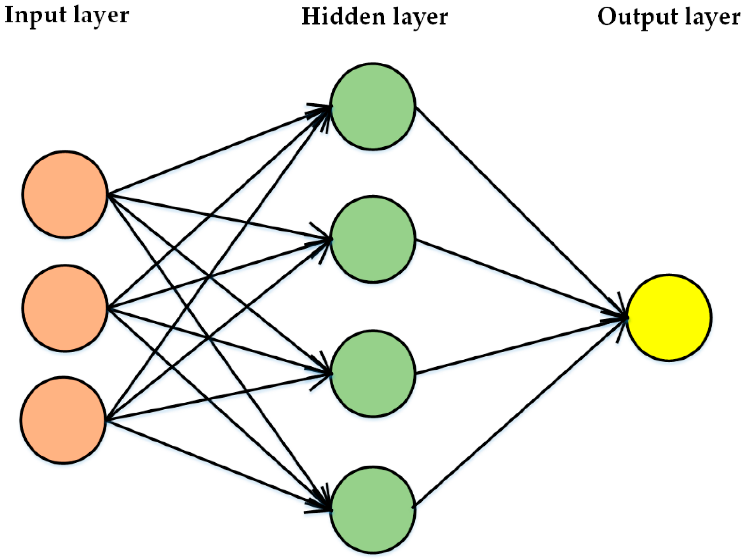
2.1. Artificial Neural Network Models

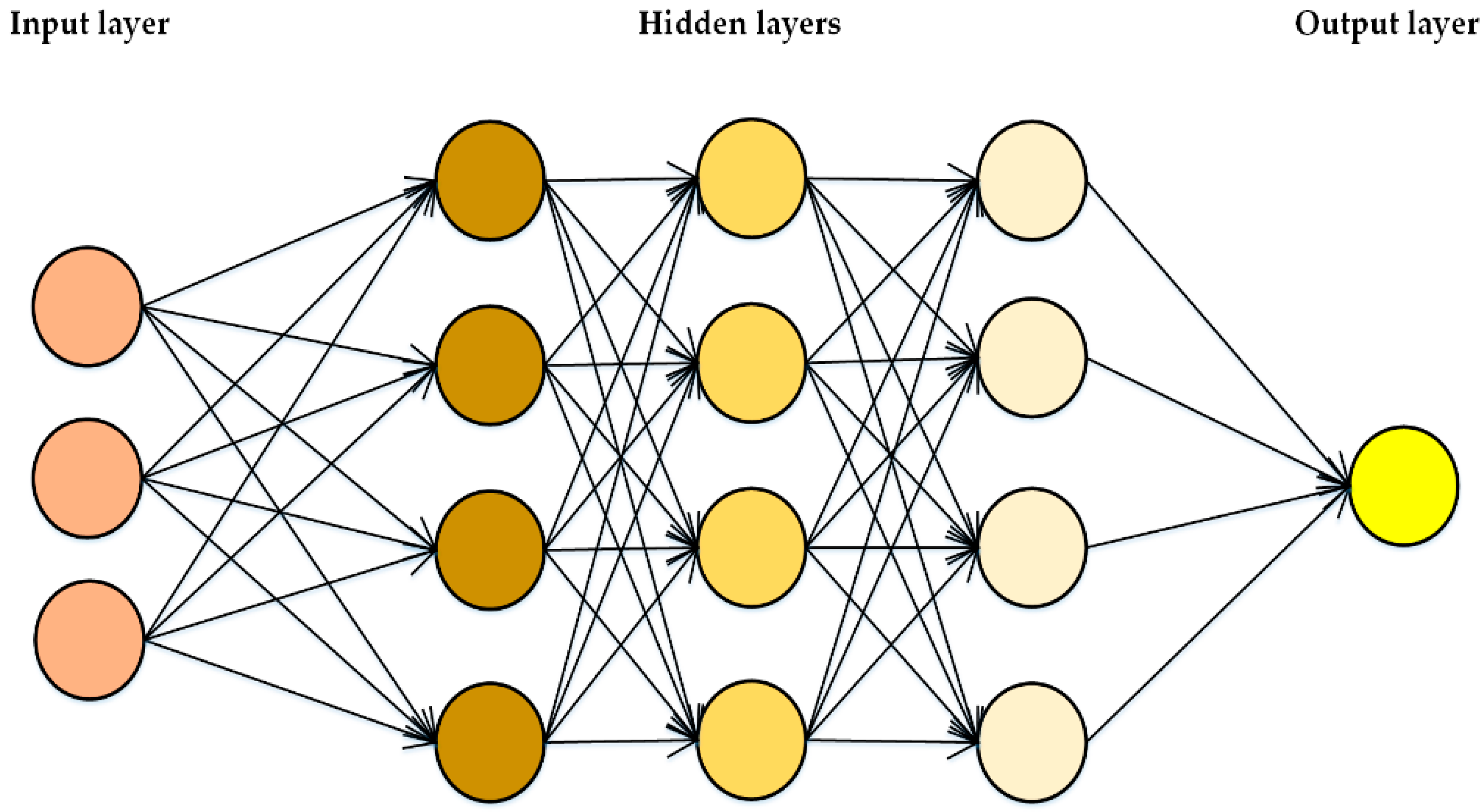
Artificial neural networks (ANNs) are a class of machine-learning models that draw inspiration from the structural and functional characteristics of the human brain [35]. These models are composed of interconnected computational units, often termed nodes or artificial neurons, which are typically organized into three main layers, as shown in Figure 1: input, hidden, and output [35]. Data are transmitted from the input to the output layer through a feedforward process, enabling the network to model complex nonlinear relationships via activation functions such as sigmoid, Rectified Linear Unit (ReLU), and hyperbolic tangent (tanh) [36].

After generating predictions, the discrepancy between the predicted and actual outputs is quantified using a loss function. The network then employs the backpropagation algorithm to iteratively adjust the connection weights, thereby minimizing the error. Repeated over numerous training epochs, this optimization procedure progressively improves the predictive performance of the network [36].

ANNs are capable of mapping nonlinear connections among inputs and outputs without the need for explicit physical concepts [37,38]. In addition, these models have a comparatively minimal computational cost because of their one-time calibration [39] and can deal with large datasets due to their separate training processes in the input-hidden and hidden-output components.

ANNs are the most popular type of ML model for estimating hydrological components (e.g., SM). For instance, Satalino et al. [40] employed an ANN trained using data from the Integral Equation Model (IEM) to assess SM retrieval and the impact of error sources on the performance of the model. The overall Root Mean Square Error (RMSE) of the predicted SM was 6%, and the main source of error was the soil roughness parameter, which highly affected the relationship between the SM content and the radar backscattering coefficient. Notarnicola et al. [41] employed a trained ANN model using backscatter and emissivity data and showed that ANNs provide a reasonable balance between stability, accuracy (with an average R² value of 0.8), and computational speed compared to widely used inversion strategies, such as the simplex algorithm and the Bayesian method. An ANN model with the learning method of back propagation was employed by Arif et al. [42] to forecast SM using input data of reference ET and precipitation in a paddy field. The results indicated the reliability of the ANN model in estimating SM with R² values of 0.8 and 0.73 for training and verification processes, respectively.

Additionally, Elshorbagy and Parasuraman [43] found that a higher-order neural network model trained using air temperature, soil temperature, net radiation, and precipitation outperforms a conceptual model for SM estimation. Moreover, this study concluded that the surface temperature was the most effective variable for SM estimation. Hassan-Esfahani et al. [26] employed a three-layered Feed-Forward Neural Network model for estimating SSM using remotely sensed data, including vegetation indices, visual, near-infrared, and thermal data, as well as field capacity. The results revealed acceptable performance of the model compared to field measurements with RMSE, Mean Absolute Error (MAE), coefficient of correlation (R), and coefficient of performance values of 2.0, 1.8, 0.88, and 0.75, respectively. According to [44], SM was predicted using an Extreme Learning Machine (ELM), a simple single-hidden layer feedforward NN with suitable generalization ability and high learning speed, and SVM by weather factors and previous SM time series. Compared with SVM, ELM showed higher accuracy with a greater prediction range and learning speed. Li et al. [45] applied an ANN model trained with evapotranspiration, SM, and precipitation to estimate SM and reported that a simple three-layer FFNN has a higher estimation accuracy and lower computational cost, in addition to the lack of need for accurate prior knowledge compared to physical models. Paul and Singh [46] employed an ANN to modify the effectiveness of the hydrological model and found that the predicted SMs had similar behavior to the observed ones. Paloscia et al. [47] employed the integration of an ANN model and the advanced integral equation model (AIEM) to estimate SM content from Advanced Synthetic Aperture Radar (ASAR) and RADARSAT2 images. Different configurations, including Vertical and Horizontal (VH) and Vertical and Vertical (VV), were used to evaluate the model. The retrieval accuracy (RMSE) for SM content varied between 0.02 m³/m³ when only VH polarization was present and 0.06 m³/m³ when only VV polarization was available.

Baghdadi et al. [48] used a Multilayer Perceptron (MLP) model with a dataset simulated by the IEM to estimate SM and surface roughness using inversion. By considering a priori understanding of the soil variables, the performance of the NNs was evaluated for several inversion cases. RADARSAT-2 images were employed to verify the inversion approach. According to the findings, the RMSE for SM was 0.098 cm³/cm³ without pre-existing knowledge and 0.065 cm³/cm³ with a priori report. Baghdadi et al. [49] assessed the effectiveness of the MLP model in estimating surface roughness and SM by employing the backscattering coefficient at different angles and achieved RMSE values of 7.6% and 0.47 cm for SM and surface roughness, respectively.

Singh and Gaurav [50] employed a fully connected feed-forward ANN with a structure of 9-5-5-5-1 to estimate surface soil moisture by utilizing multi-sensor remote sensing images. The analysis identified Longitude, Vertical–Vertical (VV), and Vertical–Horizontal (VH) backscatter images as the most relevant input features for mapping soil moisture, with Longitude showing a negative impact and VV showing a positive impact, while VH exhibited inconsistent trends. The study found that the digital elevation model (DEM) positively influenced soil moisture, whereas Latitude had a negative effect. The ANN demonstrated high predictability for surface soil moisture compared to other benchmark algorithms, although it faced a trade-off between performance and computational time complexity. The framework generated a surface soil moisture map using dual-polarized backscatter images from Sentinel-1, along with red and near-infrared reflectance from Sentinel-2 and DEM data from the Shuttle Radar Topography Mission (SRTM). The ANN model effectively predicted SM, surpassing all benchmark algorithms with a correlation coefficient of 0.80, an RMSE of 0.040 m³/m³, and a bias of 0.004 m³/m³.

Nadeem et al. [51] developed downscaling approaches using ML techniques to enhance the spatial resolution of low-resolution microwave SM data by integrating optical and thermal infrared observations of surface variables. The research utilized two ML algorithms, RF and ANN, to establish relationships between low-resolution SMAP SSM and high-resolution surface variables from MODIS datasets. Four downscaling combinations were tested, with the RF + Terra model yielding the best performance, showing high correlation and lower errors at various scales. The analysis highlighted the impact of vegetation type on downscaled SM accuracy, with RF models performing better than ANN models across different vegetation covers. The study also addressed gaps in original SMAP SM data due to clouds and freezing conditions, achieving high-resolution gap-filled SM estimates. The RF + Terra model outperformed ANN + Terra in accuracy, capturing spatial distribution patterns effectively. While the downscaling techniques provided valuable high-resolution SM data, the necessity for bias correction in extreme values for hydrological applications was emphasized.

A study [52] analyzed the relationship between satellite reflectance and soil water content, revealing a nonlinear trend where reflectance first decreased and then increased with rising moisture levels. Vegetation indices, including ratio, difference, and normalized difference vegetation indices from GF-6 and Landsat 8, showed strong correlations (r > 0.8) with soil water content, though regression models exhibited underfitting. Nonlinear models, particularly extreme learning machine and random forest outperformed linear models, with the out-of-bag random forest (OOB-RF) model achieving the highest accuracy (R² = 0.852 for calibration and R² = 0.834 for prediction). The model also demonstrated stability, with RMSE values of 3.013% and 3.317% for calibration and prediction datasets, respectively. These findings confirm the feasibility of using multispectral remote sensing and OOB-RF modeling for accurate soil water content estimation.

Vahidi et al. [53] integrated a drone-mounted hyperspectral sensor (L-Pika) with ML algorithms to assess soil moisture at various depths in vegetated corn fields. Principal Component Analysis (PCA) effectively identified key spectral variables, which were then used in an ANN model for soil moisture estimation. The ANN model outperformed other ML algorithms, particularly in estimating moisture at 30 cm depth under non-irrigated or high-water-stress conditions. Environmental factors like rainfall and air temperature variations weakened the relationship between canopy spectral data and soil moisture, increasing estimation errors. The study confirmed a significant correlation between root zone water content and canopy reflectance, especially at critical depths for plant health, highlighting spectral data’s potential as a reliable proxy for soil moisture. Certain wavelengths responsive to chlorophyll and water stress were particularly informative, providing insights for improving spectral analysis and enhancing soil moisture monitoring for precision agriculture.

Some studies have used the ANN approach with limited experimental information without simulated data. For example, Prasad et al. [54] estimated three target parameters, including the Leaf Area Index (LAI), crop biomass, and SM, by utilizing two versions of the radial basis function NN (RBFNN) trained by X-band scatterometer measurements. With RMSE of 0.01 kg/m², 0.01, and 0.03 m³/m³ for biomass, LAI, and SM, respectively, the model’s performance in estimating biomass and LAI was found to be better than SM. Xie et al. [55] developed 18 types of neural networks using the back-propagation learning algorithm (BPNN) to retrieve SM content using the Advanced Microwave Scanning Radiometer for EOS (AMSR-E) measurements. The 18.7-GHz band and vertical brightness temperature, unlike the 36.5-GHz band and horizontal brightness temperature, improved the estimation accuracy of SM. Moreover, the BPNN models driven by the brightness temperature data at 6.9 GHz and 10.7 GHz bands showed the highest performance in estimating SM with RMSE of 10.3% and R-value of 0.5. Pasolli et al. [56] made a comparison between the ANN algorithm and Support Vector Regression (SVR) in terms of SM estimation by C-band scatterometer data. Although both methods exhibited suitable performance, SVR showed higher stability and robustness under conditions with outliers and limited reference training data. This implies that an extensive reference dataset is necessary for ANN training.

To evaluate the ANN’s performance against the other statistical and iterative methods, Paloscia et al. [57] used the Bayesian method and the Nelder–Mead simplex algorithm. The results showed that the ANNs performed better than the other two methods based on computational speed and complexity. In another study, the performance of an ANN was compared with that of multivariate regression and fuzzy logic in SM estimation. Considering RMSE and R² values equal to (3.39%, 0.77), (3.45%, 0.76), and (4.48%, 0.72) for ANN, fuzzy logic, and multivariate regression, respectively, the performance of the fuzzy logic and NN models was better than that of multiple regression. Furthermore, the use of soil and NDVI information, in addition to microwave data, led to an improvement in the RMSE statistics for SM estimation by 30% [58].

In addition to estimating soil moisture, ML methods are utilized to downscale the data from sensors with varying levels of resolution. For example, Srivastava et al. [59] investigated three artificial intelligence methods, including ANN, SVM, and Relevance Vector Machine (RVM), along with a Generalized Linear Model (GLM) to downscale the spatial resolution of SMOS soil moisture products using Moderate Resolution Imaging Spectroradiometer (MODIS) Land Surface Temperature (LST). R², bias, and RMSE were obtained as (0.751, 0.628, and 0.011), (0.691, 1.009, and 0.013), and (0.698, 2.370, and 0.013) for the ANN, RVM, and SVM, respectively, showing the best performance of ANN followed by RVM and SVM. Alemohammad et al. [60] retrieved high spatial-resolution SM data by establishing the relation among high-resolution NDVI and coarse-resolution SM products through an ANN. Compared with in situ observations, downscaled SM estimates had higher accuracy than the SM obtained from SMAP. Senanayake et al. [61] tested an ANN, Regression Tree (RT), and Gaussian Process Regression (GPR) according to soil thermal inertia theory to downscale SMAP, SMOS, and AMSR-E soil moisture products by employing MODIS LST, NDVI, soil clay content, and in situ SM measurements. Downscaled soil moisture showed RMSEs of 0.03, 0.09, and 0.07 cm³/cm³ against airborne observations and unbiased RMSEs of 0.07, 0.08, and 0.05 cm³/cm³ against in situ measurements for RT, ANN, and GPR models, respectively.

The application of ANNs in small areas is limited because poor simulations occur outside the range of training data. However, training ANNs using SM data from different areas can improve estimation accuracy over large areas. For example, Gill et al. [62] achieved good estimates of soil moisture for an independent station using ANNs driven by data from ten stations in the same area.

In addition to SSM estimation, ANNs can be used to model RZSM. For example, an RZSM estimation algorithm employing an ANN model was developed by Jiang and Cotton [27]. They applied an ANN model, which is a combination of Self-Organizing Feature Maps (SOFM) and Grossberg linear networks [63] to the Normalized Difference Vegetation Index (NDVI), infrared skin temperature, and precipitation as primary independent inputs. The results indicated a strong correlation among the ANN estimations and the Mesonet observations, particularly for spatially averaged data. This study concluded that the ANN model holds promise as an effective alternative for SM estimation. One notable benefit of the ANN is its capability to provide estimates with a resolution compatible with remotely sensed infrared data, thus offering a possibility for global coverage. Gu, Zhu [64] evaluated the performance of an ANN in predicting the RZSM during the growing season and, thereby, in irrigation scheduling using process-based simulations. Rooting depth, climatic information, and soil moisture were used as input data to simulate the daily soil moisture at various depths. Although the model exhibited adequate performance in the prediction of soil moisture with minor errors, the scheduling efficiency decreased due to large errors under water-stressed conditions. However, the ANN ensemble model improved the accuracy of SM prediction and scheduling. Kornelsen and Coulibaly [65] built a prediction model of the RZSM based on SSM obtained from a multilayer perceptron. Their findings demonstrated the power of ANNs in representing the RZSM dynamics for the testing sites. However, the model performance was poorer than that of in situ measurements outside the training conditions. Souissi et al. [66] used an ANN model to estimate the RZSM using in situ SSM observations on a global scale. Because the elimination of networks with lower contributions led to an increase in accuracy, a data filtering approach was employed based on the model’s performance, which improved the mean Nash–Sutcliffe Efficiency (NSE) by 42.5% and a mean correlation of 20.5%. Souissi et al. [67] investigated the impact of various process-related inputs in the prediction of RZSM (depth between 30 and 55 cm) using the ANN model proposed by Souissi et al. [66]. The input variables included land surface temperature, NDVI, evaporation efficiency, and soil water index achieved using a recursive exponential filter. The results showed that the process-based features improved the general effectiveness compared to the reference model implemented using only SSM features. Moreover, the feasibility of ANNs to obtain RZSM was evaluated in [68] using soil texture, air temperature, land surface temperature, snowfall, rainfall, and SSM at a continental scale. According to the results, ANNs, with a correlation coefficient of 0.7, outperformed in retrieving SM at 20 cm compared with that at 50 cm. In addition, the use of soil texture data promoted the performance of the model, particularly in estimating RZSM at 50 cm.

Table 1. A list of studies utilized ANNs to estimate soil moisture.

Research	Models	Input	Output	Performance Criteria	Year of Study
Satalino et al. [40]	IEM, NNs	Relative dielectric constant, roughness	SM	Root Mean Square (RMS)	2002
Baghdadi et al. [49]	MLP	Surface roughness, SM, backscattering coefficients	SM, surface roughness	RMSE, MAE, Bias, Index of Agreement (IoA)	2002
Jiang and Cotton [27]	ANN	Precipitation, NDVI, infrared skin temperature, SM	RZSM	R, RMSE, Bias	2004
Gill et al. [62]	ANN, SVM	Air temperature, relative humidity, average solar radiation, soil temperature, soil temperature	SM	RMSE, MAE, R	2006
Notarnicola et al. [41]	ANN	Backscattering coefficients and emissivity	SM, dielectric constant	Mean Square Error (MSE), Mean Absolute Deviation (MAD), Mean Relative Error (MRE)	2008
Elshorbagy and Parasuraman [43]	ANN	Air temperature, soil temperature, net radiation, ground temperature, precipitation	SM dynamics	RMSE, Mean Absolute Relative Error (MARE), R	2008
Paloscia et al. [57]	FFNN, Bayesian method, Nelder–Mead simplex algorithm	SM, surface roughness, vegetation parameters (plant height, density, leaf number, leaf dimension, fresh biomass), backscattering coefficients	SM, surface roughness, vegetation parameters	R2, Mean Error (ME)	2008
Prasad et al. [54]	Conventional RBFNN and generalized regression neural network (GRNN)	Backscattering coefficients	SM, biomass content, LAI	Time series analysis	2009
Lakhankar et al. [58]	ANN, fuzzy logic	NDVI, Vegetation Water Content (VWC), Vegetation Optical Depth (VOD), backscatter, soil texture, SM	SM	RMSE, R	2009
Xu et al. [69]	ANN combined with Xinanjiang model	Precipitation, pan evaporation	SM	Time series analysis	2010
Pasolli et al. [56]	MLP, SVR	Passive and active microwave measurements	SM	MSE, MRE, R2	2011
Baghdadi et al. [48]	MLP	Surface height, SM, backscattering coefficients	SSM, surface roughness	RMSE, Bias	2012
Arif et al. [42]	ANN	Evapotranspiration, precipitation	SM	R2	2013
Paloscia et al. [47]	ANN	Backscattering coefficients, incidence angle, NDVI	SM	Timeliness, RMSE	2013
Srivastava et al. [59]	ANN, SVM, RVM, GLM	Evapotranspiration, land surface temperature, SM, rain gauge and river flow data	Land surface temperature, SM	R2, Bias, RMSE	2013
Liu et al. [44]	ELM, SVM	Rainfall, air temperature, relative humidity, wind speed, solar radiation, SM	SM	MAE	2014
Kornelsen and Coulibaly [65]	ANN	SM, temperature, relative humidity, solar radiation, wind speed, evapotranspiration, antecedent precipitation index, silt and clay content, leaf area index	RZSM	RMSE, R	2014
Xie et al. [55]	BPNN	Brightness temperature at different polarizations	SSM	RMSE, R	2014
Hassan-Esfahani [26]	ANN	Optical, NIR, and thermal imagery, NDVI, Vegetation Condition Index (VCI), Enhanced Vegetation Index (EVI), Vegetation Health Index (VHI), field capacity	SSM	RMSE, MAE, R, R2	2015
Pan et al. [68]	ANN	Soil texture, SSM, and the cumulative values of air temperature, surface soil temperature, rainfall, and snowfall	RZSM	RMSE, ubRMSE, R	2017
Alemohammad et al. [60]	ANN	SMAP soil moisture observations, NDVI, topographic index or topographic wetness index, SM	SSM	R2, unbiased Root Mean Square Difference (ubRMSD), Coefficient of Variation (CV)	2018
Li et al. [45]	ANN	SM, potential evapotranspiration, precipitation	SM	RMSE, NSE, SD	2020
Souissi et al. [66]	ANN	Evapotranspiration, soil texture, SSM, air temperature, surface soil temperature, rainfall, snowfall	RZSM	RMSE	2020
Senanayake et al. [61]	RT, ANN, GPR	LST, clay content, NDVI	SSM	RMSE, unbiased Root Mean Square Error (ubRMSE)	2021
Gu et al. [64]	ANN	Climatic data, rooting depth, SM	RZSM	R2, Normalized Mean Bias Error (NMBE), Normalized Mean Absolute Error (NMAE), Normalized Root Mean Square Error (NRMSE)	2021
Souissi et al. [67]	ANN	Vegetation stress, water storage change, SSM, NDVI	RZSM	RMSE, R	2022
Singh et al. [50]	ANN, Generalised Regression Neural Network (GRNN), Radial Basis Network (RBN), Exact RBN (ERBN), Gaussian Process Regression (GPR), SVR, RF, Boosting Ensemble Learning (Boosting EL), RNN, Binary Decision Tree (BDT), and Automated Machine Learning (AutoML)	Rainfall, air temperature, relative humidity, spectral data, soil moisture	SSM	R, RMSE, Bias	2023
Nadeem et al. [51]	ANN, RF	Soil moisture, soil temperature, and precipitation	SM	R, Bias, RMSE, unbiased (ubRMSE)	2023
Chen et al. [52]	ELM, RF, out-of-bag and random forest (OOB-RF)	Soil water content	SM	R2, RMSE, and relative percent deviation (RPD)	2025
Vahidi et al. [53]	ANN, SVM, RF, Gradient Boosting (XGBoost)	Rainfall, air temperature, spectral data, soil moisture	SM	RMSE, R2, percent bias (PBIAS) and Bayesian Information Criterion (BIC)	2025

provides a detailed list of these studies.

Although ANNs have proven to be effective at extracting features within big datasets, they tend to concentrate on individual data attributes, often ignoring the dynamic temporal and spatial patterns of soil moisture that may result in a reduction in the accuracy of predictions. With this in mind, enhancing the depth of neural networks can lead to improved model representation, as exemplified by deep-learning models. These deep-learning models are elaborated upon in the subsequent section.

ANNs are highly effective in modeling complex, nonlinear relationships in SM prediction, especially when using diverse inputs such as remote sensing data, meteorological variables, and vegetation indices. They offer advantages like high accuracy, fast computation after training, flexibility in structure, and robustness against noise. ANNs are also suitable for both surface (SSM) and root zone soil moisture (RZSM) estimation and can outperform traditional models and other machine-learning algorithms in many cases.

Despite their strengths, ANNs often require large, high-quality training datasets, and their performance degrades when extrapolating beyond trained conditions. They are sensitive to overfitting and sometimes computationally intensive during training. Moreover, ANNs may struggle to generalize across different geographic regions or soil types without regional retraining or data normalization.

Key challenges include limited interpretability, dependency on diverse and high-resolution datasets, and poor performance in data-scarce or extreme conditions. Integrating multisource data (e.g., radar, thermal, optical) and ensuring model transferability across spatial and temporal scales remain active areas of research. Additionally, the need for bias correction in downscaling applications and model robustness across vegetation covers and weather variability is significant.

2.2. Deep Learning

Deep-Learning (DL) models are a subset of ANNs with multiple hidden layers, often more than three layers, as shown in Figure 2, enabling them to deal with big multi-feature data [70]. Despite traditional neural network models that suffer from slow training processes, limited generalization ability and scalability, and a high possibility of falling into local optima, DL models can rapidly process data with high computational efficiency and accuracy estimation. They can automatically learn hierarchical representations of data and derive high-level features from low-level input data by capturing intricate nonlinear relationships [71]. Moreover, these models can improve prediction accuracy by integrating more data through additional learning. However, training deep-learning models typically requires large datasets, which can limit their application under data-scarce conditions.

The primary DL models frequently employed for hydrological forecasting encompass spatial approaches (such as Convolutional Neural Networks or CNN, introduced by LeCun and Bengio [72], temporal approaches (such as Long Short-Term Memory networks or LSTM, as pioneered by [73], and models that combine spatial and temporal aspects (such as Convolutional LSTM or ConvLSTM, developed by Shi et al. [74]. Various studies have used these variants to determine the spatiotemporal distribution of soil moisture. For example, Sobayo et al. [75] employed a CNN model because of its ability to recognize images to establish the relationship between the soil temperature obtained from thermal images and soil moisture for the prediction of SM. The developed model outperformed a typical Deep Neural Network (DNN). Tseng et al. [76] compared the performance of CNN with several ML methods, including linear SVMs, Random Forests (RFs), and two-layer Neural Networks, in deriving local SM conditions from aerial agricultural imagery. Among all the models, CNNs exhibited the best performance (with a normalized mean absolute error of 3.4%). As the layers decrease in number, the CNN’s accuracy for extracting features decreases, as observed in [77]. To address this challenge, He et al. [78] introduced the concept of residual networks (ResNet) by incorporating residual blocks into the construction of deep neural networks.

Unlike CNNs that utilize convolutional layers to capture spatial characteristics from the data, LSTM models employ recurrent layers with memory cells to extract temporal relationships in sequential data. These models, as a kind of recurrent neural network (RNN), can preserve valuable information from historical time-series data over an extended period and predict nonlinear systems with minimal inputs [73,79,80]. Numerous researchers have exploited the LSTM model to estimate and predict soil moisture. For example, Fang et al. [81] used the LSTM model to simulate SMAP soil moisture using atmospheric forcing variables and SM data obtained from the outputs of Noah’s hydrologic model. The results showed a high R and low RMSE between simulations and observations. In addition, the study demonstrated a better performance of LSTM than conventional methods in predicting SSM. Adeyemi et al. [82] exploited the LSTM model trained by precipitation, climatic data, and past SM information to predict volumetric SM content one day ahead and compared it with SM estimated by traditional FFNNs as well as in situ measurements, which led to an R² of more than 0.94. Moreover, water savings varying between 20% and 46% were obtained from the predictive system combined with the Dynamic Neural Network models, while water use efficiency and yield productivity were close to those of the rule-based system. Fang et al. [83] proposed a predictive model to forecast the SMAP SSM product using the LSTM model trained with static physiographic attributes, atmospheric forcing variables, and fluxes simulated by LSMs. The results revealed that the model captured the interannual trends of the RZSM well. However, the performance of the model was restricted by the SMAP in some cases because of the shallow sensing depth. In addition, the Noah-LSTM combination outperformed the land surface approach and confirmed the importance of LSTM-extended SMAP data. Fang and Shen [84] applied LSTM to simulate interannual trends of soil moisture using climatic and static physiographic data, which led to an improvement in estimating near-real-time global SM. Furthermore, Cai et al. [13] developed a two-hidden-layer SM prediction model based on a DNN regression algorithm (DNNR) using 0–20 cm depth SM and meteorological data. They determined the efficiency and generalization capability of deep learning for SM prediction with high accuracy (20%).

Although RNNs are effective for modeling time-series data by maintaining information from past time steps through internal self-looped cells [85], they face the challenge of gradient disappearance, particularly in handling long-range dependencies. To address this issue, a gate mechanism was introduced in RNN-based LSTM models, as described by Hochreiter and Schmidhuber [73]. However, LSTM models tend to overlook the acquiring knowledge from backward features, which has resulted in the creation of a bidirectional LSTM (BiLSTM) network model that integrates both backward and forward LSTMs [61]. By combining the BiLSTM and ResNet models, a novel SM prediction model, ResBiLSTM, was developed to extract bidirectional and high-dimensional spatiotemporal features [79]. To build the multi-depth SM prediction model, SM, meteorological, and growth data were used to train the model. The results demonstrated that ResBiLSTM outperformed the classical ML models and deep-learning models in predicting the meteorological and SM data at all growth stages.

Despite the advantages of artificial intelligence in capturing nonlinear functions, they mostly detect temporal variations in soil moisture, while eco-hydrological variables are correlated to both space and time. Therefore, Mao et al. [80] solved this problem using the ConvLSTM model, which is a combination of LSTM and CNN models. ConvLSTM utilizes output from the previous layer as input for the next layer, enabling the concurrent extraction of spatiotemporal features through the convolution layer while maintaining the original map size. This model was first developed by Shi et al. [74] to predict the spatial and temporal properties of rainfall, and it exhibited better performance than cutting-edge precipitation forecasting algorithms [86] and Fully Connected LSTM [87] for predicting rainfall intensities.

Mao et al. [80] estimated RZSM by using spatiotemporal continuous RZSMs obtained from the Hydrus-1D model, soil characteristics (such as bulk density, textural composition, and soil organic matter content), vegetation indices (EVI, NDVI, and LAI), meteorological conditions (precipitation and evapotranspiration), and SM data from the Global Land Data Assimilation System (GLDAS). According to the results, the ConvLSTM model improved the RZSM estimates compared to the GLDAS products. Furthermore, a combination of artificial intelligence and physical models as an innovative framework based on machine learning with two layers provides a platform to simulate the spatiotemporal distribution of RZSM with acceptable accuracy on a large scale. Recently, Li et al. [88] used LSTM, CNN, and ConvLSTM models to simulate daily SM using limited SMAP samples. The results showed that the ConvLSTM model outperformed the other models, with an R² ranging from 0.909 to 0.916. ElSaadani et al. [89] applied the ConvLSTM model to predict SM using hydrometeorological forcing variables. It was found that the model outperformed CNN with an R-value of 0.9 and an RMSE of 2.5%. Moreover, the model was able to fill the gaps between discrete SM observations.

Cai et al. [13] developed the use of DNNR with a significant ability of big data fitting to develop an SM predictive model. The selected meteorological inputs—which contribute effective weights for predicting the moisture—were air pressure, air temperature, relative humidity, wind speed, surface temperature, precipitation, and SM. The results confirmed the practicality and efficiency of the deep-learning model for predicting SM. Its generalization capabilities and robust data fitting enhanced the characteristics of inputs, ensuring precise predictions of SM values and trends.

In addition, Diouf et al. [90] employed a DNNR model to simulate the spatiotemporal distribution of soil moisture for the two first layers by dewpoint temperature, air temperature, wind speed, evaporation from bare soil, SM at depths of 0.07 and 0.21 m, surface sensible heat flux, and initial SM. The prediction accuracy was greater than 93%.

Another study [91] demonstrated the potential of ML and DL models for predicting soil moisture in wheat fields using Synthetic Aperture Radar (SAR) data. By integrating satellite remote sensing with computational techniques, models such as SVM, RVM, RF, ANN, and CNN were evaluated, with RF emerging as the most effective in handling complex environmental datasets. DL models, particularly CNNs, leveraged spatial analysis but showed varying success across test scenarios. The research enhanced soil moisture prediction accuracy, aiding precision agriculture through improved irrigation and water management strategies. Emphasizing continuous monitoring and model updates, the study highlighted the scalability of ML and DL for broader agricultural applications.

Nijaguna et al. [92] presented a novel technique for soil moisture retrieval, which involves several key phases. Initially, images were acquired, and vegetation indices (NDVI, green leaf area index (GLAI), green NDVI (GNDVI), and water-deficit reflectance vegetation index (WDRVI)) were derived. An improved water cloud model (WCM) was then implemented to rectify the impact of vegetation. Soil moisture was subsequently retrieved using Deep Memory Networks (DMN) and Bi-directional Gated Recurrent Units (Bi-GRU), with their outputs combined through enhanced score-level fusion to yield final results. The study found that the RMSE for the combined Hybrid Classifier (HC) method using Bi-GRU and DMN is lower (0.9565) compared to various HC methods without vegetation indices or with conventional water clouds. Similarly, the Mean Error (ME) for the combined HC method is also less (0.728697) than the other methods analyzed.

It should be emphasized that DL models operate not only structurally but also mechanistically in the context of soil moisture prediction. In CNNs, small convolutional kernels scan multi-channel spatial inputs (e.g., soil moisture maps, vegetation indices, elevation) to extract localized features such as moisture gradients or texture variations. Deeper layers hierarchically combine these into higher-order spatial representations, while pooling layers reduce dimensionality and highlight dominant structures. These spatial features are then fused with temporal data to model joint spatiotemporal relationships.

In LSTM networks, the forget gate discards irrelevant past information (e.g., transient post-rainfall spikes), while the input gate integrates relevant new drivers (e.g., precipitation, evapotranspiration) into the cell state. The memory cell maintains and updates the internal state by combining past and current information, capturing both short-term responses and long-term trends. The output gate determines which information is passed forward for prediction. This gated mechanism allows LSTMs to effectively learn complex hydrological dependencies and reduce noise in SM time series [93]. A list of studies on SM retrieval using DL models is presented in

Table 2. Studies conducted to model soil moisture using DL techniques.

Research	Models	Input	Output	Performance Criteria	Year of Study
Fang et al. [81]	LSTM	SMAP level-3 moisture product, atmospheric forcings (precipitation, temperature, radiation, humidity, and wind speed), model-simulated moisture, static physiographic attributes	SSM	R2, RMSE, Bias	2017
Sobayo et al. [75]	CNN, DNN	Soil temperature	SM	RMSE, MARE, R2	2018
Tseng et al. [76]	SVM, RF, ANN, CNN	Synthetic Red–Green–Blue (RGB) aerial image	SM	Median absolute error	2018
Adeyemi et al. [82]	LSTM	SM, precipitation, climatic measurements	Temporal SM fluxes	R2, RMSE, MAE	2018
Fang et al.l. [83]	LSTM	Atmospheric forcing data, static physiographic attributes	SSM, RZSM	RMSE, Bias, R, ubRMSE	2018
Mao et al. [80]	ConvLSTM	Soil properties (bulk density, clay content, and sand content), Land Use Land Cover (LULC), soil temperature, vegetation water content, vegetation opacity, roughness coefficient	RZSM, brightness temperature	R, ubRMSE	2019
Cai et al. [13]	DNNR	Meteorological data (air pressure, air temperature, relative humidity, wind speed, surface temperature, precipitation), soil moisture	SM	MAE, MSE, RMSE, R2	2019
Fang et al. [84]	LSTM with a novel data integration kernel	Climatic forcing time series, static physiographic attributes	SM	Time-averaged difference (bias), RMSE, ubRMSE, R	2020
Yu et al. [79]	ResBiLSTM	Soil and vegetation conditions, human activity, weather forecast information	SM	MSE, MAE, RMSE, Mean Absolute Percentage Error (MAPE), R2	2020
Diouf et al. [90]	DNNR	Meteorological parameters (air temperature, precipitation, dewpoint temperature, wind speed), soil properties (sensible heat flux, evaporation), soil moisture in different depths	SM	MAE, R2	2020
Li et al. [88]	CNN, LSTM, ConvLSTM	Lagged SM, soil temperature, season, precipitation	SSM	R2, RMSE	2021
ElSaadani et al. [89]	CNN, LSTM, ConvLSTM	Soil moisture, LULC, precipitation, longwave and shortwave fluxes, baseflow-groundwater runoff, storm surface runoff, moisture availability	SM	NRMSE, R	2021
Nijaguna et al. [92]	Deep Max Out Network (DMN), Bidirectional Gated Recurrent Unit (Bi-GRU), water cloud model (WCM)	NDVI, GLAI, Green NDVI, and WDRVI features	SM	ME, RMSE, MARE, MAPE	2023
Lakra et al. [91]	SVM, RVM, RF, ANN, and CNN	Soil moisture, Synthetic Aperture Radar (SAR) data	SM	RMSE, R2, Bias, R	2025

.

2.3. Kernel Models

Kernel function-embedded models are a class of ML techniques that are employed for various purposes, such as classification and regression. These models are known for their simplicity and generality, and they are particularly useful when dealing with nonlinear and complex data. However, they can require significant computational resources, especially in high-dimensional environments.

One of the widely recognized kernel techniques is the SVM model, which uses a kernel function which transforms data into a space with higher dimensions, simplifying the process of locating a linear hyperplane that separates data points. Linear, polynomial, and radial basis functions (RBF) are popular kernel functions employed in SVMs. The selection of the kernel function and its parameters can significantly influence the effectiveness of kernel models. Tuning these parameters effectively constitutes a crucial aspect of kernel methods.

SVM models (founded on statistical learning theory) can address inverse problems by projecting historical data forward to derive the variables of interest. Instead of conventional Empirical Risk Minimization (ERM), these models employ Structural Risk Minimization (SRM) through quadratic optimization, a distinctive feature that ensures a global optimum [56]. The SVM relies on the generation error bound and a rigorous loss function, resulting in highly accurate predictions [94]. Additionally, SVMs exhibit robustness to noise and the ability to generalize concepts, even when dealing with limited data scenarios [82].

Because of their rapid processing capabilities and ability to achieve satisfactory performance with a smaller training dataset, SVM models have gained considerable attention for the extraction of environmental parameters. For example, Jia et al. [95] employed SVM and RF models to predict SM content using Global Navigation Satellite System-Reflectometry (GNSS-R) data, including reflectivity, dielectric constant, elevation angle, and soil moisture. According to the results, SVM showed poorer performance than RF in retrieving SM, particularly when the type of soil was either unknown or inconsistent. Gill et al. [62] built two prediction models based on SVM and ANN to calculate soil moisture four and seven days ahead by employing SM data and meteorological data. Based on the results, SMs predicted by SVM, with an increase in accuracy to 89%, exhibited a better match with the in situ measurements than the ANN predictions.

Kahlil et al. [96] evaluated the effectiveness of a statistical-learning-theory-based SVM and sparse Bayesian-learning-based RVM in making dependable estimations. The credibility of these approaches was demonstrated by their exceptional effectiveness in predicting soil moisture.

A comparison was conducted between the two models, HYDRUS-1D and SVM, for the long-term estimation of soil water content on a daily basis at various depths using meteorological data on the current day and soil moisture on the preceding day [97]. Both models demonstrated relatively accurate predictions of SM content, especially in layers crucial for the growth of a crop, such as those close to the surface. The RMSEs for predictions of volumetric soil water content in the topsoil using the SVM model and at depths of 5, 10, and 25 cm were 0.035, 0.030, and 0.021 cm³·cm⁻³, respectively. In comparison, the physically based model yielded RMSE of 0.042, 0.049, and 0.045 cm³·cm⁻³ at the same depths. The results indicate that the SVM can be effectively employed to estimate changes in soil water content over time with comparable accuracy to that of physically based models. It should be noted that omitting the previous SM time sequence from the input dataset led to an insufficient accuracy of the results.

A data assimilation (DA) method using SVM and RVM models was implemented to estimate topsoil and surface moisture content at depths of 6 and 30 cm, respectively, through a two-step model with input data of meteorological information soil temperature, crop physiological characteristics, and soil water-holding capacity. The simulated topsoil SM (0–6 cm) was estimated and employed as a boundary condition to predict soil moisture at a depth of 30 cm. Statistical indices showed a higher estimation accuracy of the RVM with a lower computational complexity than the SVM model. Paul and Singh [46] evaluated the performance of SVM, Principal Component Analysis (PCA), linear regression, and Naïve Bayes models trained by temperature, humidity, and moisture to estimate soil moisture for a period of 12 to 13 weeks in the future. An increase in accuracy was observed when SM was estimated by employing time-series supervised learning data. Ahmad et al. [98] established a relationship between Tropical Rainfall Measuring Mission Precipitation Radar (TRMMPR) backscatter, NDVI, and SM content using an SVM model trained using past ground SM data. In addition, multivariate linear regression (MLR) and an FFNN model were employed to assess the results obtained from the SVM model. The SM estimates from SVM with correlation coefficients ranging between 0.34 and 0.77 and RMSE less than 2% were in good agreement with the results obtained from the variable infiltration capacity three-layer (VIC) model. Furthermore, the SVM model, with RMSE, MAE, and R of 1.98, 1.86, and 0.51, outperformed the ANN and MLR models in predicting soil water content. Matei et al. [99] built a data mining system that was capable of collecting weather data and predicting real-time soil moisture using SVM, ANN, k-NN, linear regression, logistic regression, decision tree, fast large margin, and RF. It was found that a system with high prediction accuracy can be utilized as a suitable data platform for agriculture under any geo-climatic condition. Hong et al. [100] employed SVM and RVM to estimate soil moisture for n number of days ahead by using meteorological data such as temperature, soil temperature, wind speed, humidity, precipitation, and solar radiation, along with the soil moisture of the previous day. The results showed a 95% correlation and an error rate of 15% for a two-week-ahead prediction of soil moisture. Liu et al. [44] investigated the performance of the SVM model with that of ELM in predicting SM for an apple orchard. Although both models were useful for future irrigation planning, ELM showed higher accuracy in prediction compared to SVM.

Wu et al. [101] utilized SVM for soil water content predictions and compared the outcomes with those of ANN in a purple hilly area. Due to their superior generalization capability and assurance of global minima for the provided training data, SVMs are expected to be used in time series analysis. The predictions aligned well with the actual soil water content records. The findings revealed that SVMs outperformed ANN models in forecasting SM.

In addition to their application in classification, SVMs can also serve regression purposes, as known as Support Vector Regression (SVR). SVR relies on the Sequential Minimal Optimization (SMO) algorithm, which includes an iterative process [100]. Comparable to SVM, the SVR model can extract nonlinear connections among input and output variables, making it a widely favored method for estimating SM. Its resilience to noise and ability to generalize in scenarios with a scarcity of reference samples contribute to its popularity [102]. Pasolli et al. [56] assessed the prediction capability of SVR and MLP networks and concluded that SVR can be a valid alternative to traditional MLP neural networks. In addition, Achieng [103] evaluated the feasibility of various ML techniques, including SVR, DNN, and ANN, in replicating the Soil–Water Retention Curve (SWRC) of loamy sand by SM and soil suction measurements. The findings reveal that the RBF-based SVR model performed better than other ML methods in the simulation of soil water content, with RMSE values of 0.006 and 0.002 cm³/cm³.

ML approaches have not been used in agricultural fields with diverse crop species or with frigid soil situated above inadequately drained geological substances. To fill this gap, Acharya et al. [104] assessed the effectiveness of SVR, MLR, RF, ANN, boosted regression trees (BRT), and classification and regression trees (CART) in predicting SM in crop fields existing in the northern Red River Valley. According to their results, RF and BRT showed the best performance, with an MAE of <0.040 m³/m³ and RMSE of 0.045 and 0.048 m³/m^3, respectively. In addition, the most effective input variables for predicting soil moisture were SM data collected from local weather stations, followed by 4-day cumulative rainfall, bulk density, saturated hydraulic conductivity, and potential evapotranspiration. Prakash et al. [105] employed various ML techniques, including MLR, SVR, and RNN, to forecast SM for time frames of 1 day, 2 days, and 7 days in advance. Comparative results indicated that MLR outperformed other techniques, yielding MSE and R² values of 0.14 and 0.975 for 1 day, 0.353 and 0.939 for 2 days, and 1.59 and 0.786 for 7 days in advance.

In another study [106], RF and SVR were employed to estimate near-surface soil moisture at a 10 m resolution in Australia’s Yanco using Sentinel-1 SAR and Sentinel-2 optical imagery from 2016 to 2020. A total of 270 features were extracted, and a seasonal feature selection approach identified the most relevant inputs for each season, with the Local Incidence Angle (LIA) as a consistently important input. Vegetation influenced feature importance, with VV backscatter more relevant in low-vegetation seasons and VH backscatter in high-vegetation seasons. The RF model outperformed SVR, achieving the highest accuracy in autumn (RMSE 0.05 m³/m³) and the lowest in winter (RMSE 0.07 m³/m³). Challenges included the reduced SAR sensitivity at high soil moisture levels and the temporal misalignment of Sentinel-1 and Sentinel-2 acquisitions. The study highlighted the potential of ML and multi-sensor data for soil moisture estimation but emphasized the need for further validation across diverse environments and improvements in temporal resolution.

Another study [107] evaluated the estimation accuracy and temporal robustness of SSM using advanced MLR algorithms, focusing on generalization ability, transfer performance, and small sample scenarios. The study found that the introduction of Radar Incidence Angle (RIA) is crucial for accurate SSM estimation with dual polarization backscattering (dual-pol σ) data, and adding multispectrum and brightness temperature features significantly improves temporal accuracy. The best estimation error achieved was 0.028 cm³/cm³ when combining dynamic and steady variables. However, MLR models exhibited poor phase transfer performance (RMSE > 0.060 cm³/cm³), though the proposed transfer strategies helped mitigate overestimation and underestimation issues, with soil parameters improving transferability. Among algorithms, Gaussian Process Regression (GPR) outperformed others in low-dimensional and small-sample cases, while neural networks (NNs) required high-dimensional features and large datasets for accurate multi-phase SSM estimation. Temporal accuracy was mainly influenced by land cover, RIA, and soil parameters, with multisource data helping to reduce surface heterogeneity effects. While dual-pol σ data performed well for estimating SSM in wheat and canola, its robustness was lower for corn and soybeans. The study emphasized the value of alternative soil data (soil organic matter (SOM) and soil texture type (STT)) in reducing sampling error uncertainties in SSM estimation.

Asadollah et al. [108] introduced a methodology for predicting SM in Iran’s Lake Urmia region by integrating Gradient Boosting (GB) and SVR into the GB-SVR technique. Using six satellite SM products as inputs, the model estimated in situ SM, with GLDAS emerging as the most consistent satellite product. GB-SVR outperformed standalone GB and SVR models, improving correlation coefficient, RMSE, and MAE by 17%, 10%, and 13%, respectively. Performance varied by climate, soil, and land use, showing higher accuracy in croplands, loam soil, and cold climate (R² = 0.86, 0.74, and 0.71) and lower performance in barren lands and clay soils. Spatial analysis indicated better results in elevated southern and western regions than in flatlands. The study demonstrated the advantages of Voting Regression (VR) in enhancing predictive accuracy and model robustness but acknowledged limitations, particularly the low number of in situ SM samples and limited regional variability.

In a study carried out by Parewai and Köppen [109], a multispectral rotocam was used to capture high-resolution soil images under controlled conditions. These images were employed to create Physically Based Rendering (PBR) materials in a game engine to simulate soil properties. Image processing techniques extracted key features, and machine-learning algorithms, including ANN, SVM, and RF, classified soil moisture levels (wet, normal, dry). The Soil Digital Twin replicated real-world behavior, with the RF model achieving 96.66% classification accuracy.

Table 3. Studies conducted to model soil moisture using kernel models.

Research	Models	Input	Output	Performance Criteria	Kernel Function	Year of Study
Khalil et al. [96]	SVM, RVM	Soil moisture, meteorological data (including relative humidity, average solar radiation, soil temperature at 5 cm and 10 cm, air temperature, and wind speed)	SM	Bias, RMSE	-	2005
Gill et al. [62]	SVM, ANN	meteorological data (air temperature, relative humidity, average solar radiation, and soil temperature at 5 and 10 cm), soil moisture	SM	RMSE, MAE, R	RBF	2006
Wu et al. [101]	SVM, ANN	Soil moisture	SM	Relative Mean Errors (RME), RMSE, CV	Linear, Polynomial, RBF	2008
Ahmad et al. [98]	SVM, ANN, MLR, VIC	Backscatter and incidence angle from TRMM, NDVI	SM	RMSE, MAE, R	RBF	2010
Pasolli et al. [56]	MLPNN, SVR	Passive and active microwave measurements acquired using various sensor frequencies, polarizations, and acquisition geometries	SM	MSE, MRE	Gaussian RBF	2011
Zaman et al. [110]	RVM, SVM	Land surface temperature, surface reflectance data, air temperature, precipitation, LAI, soil temperature, soil moisture, soil water-holding capacity	SSM	MAE, RMSE, IoA, Coefficient of Efficiency (CoE)	Gaussian kernel	2012
Lamorski et al. [97]	SVM	Air temperature, humidity, atmospheric pressure, insolation, shortwave and longwave radiation, photosynthetically active radiation, albedo, wind direction and speed, soil temperature and moisture, precipitation (type and intensity)	SM	R2, RMSE, CRM	RBF	2013
Liu et al. [44]	ELM, SVM	soil moisture, flow measurement, weather data (minimum, maximum, and average wind speed, average wind direction, rainfall, barometric pressure, solar radiation, relative humidity, air temperature	SM	MAE	Polynomial kernel function	2014
Hong et al. [100]	SVM, RVM	Meteorological data (temperature, humidity, wind speed, solar radiation, precipitation), soil temperature, soil moisture	SM	MSE, MAE, R2	RBF	2016
Matei et al. [99]	A data mining system consisting of SVM, ANN, k-NN, linear regression, logistic regression, decision tree, fast large margin, RF	Timestamp, soil moisture at three depths of 10, 30, 50 cm, air temperature, precipitation	SM	Accuracy, error	-	2017
Prakash et al. [105]	MLR, SVR, RRN	Soil moisture, soil temperature	SM	MSE, R2	Linear kernel	2018
Achieng et al. [103]	SVR, ANN, DNN	Soil moisture, soil suction	SM	RMSE, IoA, R2	RBF, linear, polynomial	2019
Jia et al. [95]	RF, SVM	Reflectivity, elevation angle, dielectric constant, soil moisture	SM	R, RMSE	RBF	2020
Paul and Singh [46]	Linear regression, SVM, PCA, Naïve Bayes	Soil moisture, soil temperature, humidity	SM	F1 Score	Linear kernel	2020
Acharya et al. [104]	CART, RF, BRT, MLR, SVR, ANN	Rainfall, soil moisture, bulk density, residue cover, soil texture, saturated hydraulic conductivity	SM	RMSE, MAE, R2	RBF	2021
Jiaxin et al. [107]	MLR: Extremely randomized trees (ET), Gaussian process regression (GPR), Generalized regression neural network (GRNN)	Soil moisture, backscattering, multispectrum, brightness temperature, land cover type, soil texture, soil organic matter, soil roughness, crop parameters, radar incidence angle (RIA)	SM	R, RMSE, MAE	Nonlinear kernel	2024
Asadollah et al. [108]	VR, GB, and SVR	Soil moisture, air and soil temperature, land cover type, soil texture, soil organic matter	SM	Correlation coefficient, RMSE, and MAE	linear, polynomial	2024
Shahriari et al. [106]	RF, SVR	Soil moisture	SM	RMSE	RBF	2025
Parewai and Köppen [109]	ANN, SVM, RF	Soil moisture, soil texture	SM	Accuracy (A), precision (P), recall (R), F1-score (F1), Matthews Correlation Coefficient	RBF, linear, polynomial	2025

provides a list of research conducted to model SM using models that incorporate kernel functions.

2.4. Hybrid Models

Despite significant advancements in addressing dynamic, nonlinear, and non-stationary data using artificial intelligence techniques, individual models may exhibit inadequate accuracy in certain hydrological simulation scenarios. Integrated prediction models have evolved to deal with the limitations of standalone methods. These models aim to enhance accuracy during both the optimization and prediction phases by leveraging the strengths of individual models.

Adaptive neuro-fuzzy inference systems (ANFIS) represent a noteworthy class of hybrid models that combines ANN and fuzzy logic (Figure 3). These models establish connections between inputs and outputs by utilizing a combination of membership functions and if–then rules.

Despite ANFIS’s ability to estimate the dynamics of target variables with minimal required inputs and satisfactory accuracy, the capacity of neural networks for long-term generalization is limited due to the spontaneous and flexible nature of fuzzy logic rules. Additionally, the inclusion of extra preprocessing steps results in the consumption of valuable time and resources in frequency-domain computations. Nevertheless, ANFIS remains one of the most widely utilized models for predicting (and simulating) hydrological components (e.g., SM). Karandish and Šimůnek [111] compared the performance of a numerical model based on physical principles, HYDRUS-2D, with that of several ML models, such as ANFIS, SVM, and MLR models, to simulate SM time series under water stress conditions. Input data for the ML methods included pan evaporation, air temperature, cumulative growth degree days, crop coefficient, irrigation depth, and water deficit. The results revealed that the HYDRUS-2D model, with an RMSE ranging from 0.54 to 2.07 mm, performed better than the SVM and ANFIS models, with an RMSE ranging from 1.27 to 1.9 mm. However, ML methods could represent an acceptable performance under data-scarce conditions, whereas process-based numerical models need a significant volume of data to provide results with low uncertainty. However, the MLR model was incapable of providing robust results, mainly due to nonlinear variations in soil moisture during the irrigation process. The ML models implemented in this study are not appropriate for all water stress conditions, leading to the need for scalable data-driven methods. With the aim of irrigation scheduling, Tsang and Jim [112] used a fuzzy neural network and artificial neural network for SM prediction using weather variables, including real-time wind speed, solar radiation, relative humidity, and air temperature. The model presented suitable SM estimates ranging from 0.13 to 0.22 m³ /m³ and improved plant coverage, leading to a 20% reduced water use.

Other hybrid models have been developed by combining SVR, ANN, SVM, and DL. For instance, Ahmed et al. [113] used a combination of CNN, gated recurrent unit (GRU), as a modified type of LSTM, complete ensemble Empirical Mode Decomposition with adaptive noise (CEEMDAN), and an improved version of empirical mode decomposition (EMD), which can establish a dynamic breakdown of the predictor variables that adjusts itself. The results demonstrated that the CEEMDAN-CNN-GRU model outperformed the standalone as well as other hybrid models. A novel hybrid learning structure based on the divide-and-conquer principle was developed by Liu et al. [114] to forecast SM time series. The results showed good agreement with SM observations and greater accuracy compared to the SVM and ANN single-stage models. Dawson et al. [115] combined a multilayer perceptron basis function (MLPBF), which is a modified version of the feedforward MLP network, with an IEM using an ANN. The model was utilized to use POLARimetric SCATterometer (POLARSCAT) data, and an RMSE of 0.034 m³/m³ was achieved in comparison with the in situ SM measurements. Jin et al. [116] employed a support vector area-to-area regression kriging (SVATARK) model, which is a combination of SVR and area-to-area kriging, to downscale the European Space Agency (ESA) SSM product. The results indicated that RMSEs varied from 0.04 to 0.076 m³/m³ against ground-based observations. In a study conducted by Ronghua et al. [117], a multilayer neural network with multi-valued neurons (MLMVN) modified by principal component analysis (PCA) was used to predict SM by using soil moisture, rainfall, temperature, and wind speed as input data. The results demonstrated that the modified model outperformed the MLMVN model for the long-term SM prediction. Pasolli et al. [118] integrated the SVR model with a novel multi-objective selection strategy to estimate the SM content using fully polarimetric RADARSAT-2 images. The accuracy of the SM prediction, with an RMSE of 0.0485 m³/m³, was improved due to the use of polarimetric features.

Although NN models can approximate complex nonlinear processes by generating robust functions [81], traditional FFNNs limit the learning capability in simulating dynamic data, leading to suboptimal predictions [84]. Temporal data can be used in ANNs through LSTM, RNN, CNN, and multitemporal averaging. For instance, Souissi et al. [66] employed an ANN model trained by temporally averaged surface soil moisture to predict the RZSM across different climatic conditions, resulting in a correlation of 0.77. In addition, Breen et al. [30] used a hybrid ANN that integrated LSTM and MLP networks to predict near-surface SM using static and dynamic input data. LSTM and MLP were employed to incorporate dynamic weather and static spatial data during the training process. According to the results, the simulated SMs were comparable to the SMAP data.

To address the generalization challenges of traditional standalone models, optimization techniques such as the genetic algorithm (GA) [119], Grey Wolf Optimizer (GWO) [120], and particle swarm optimization (PSO) [121,122] are incorporated into the models to build robust knowledge-driven predictive systems. Thus, several researchers have tackled the absence of optimization algorithms by creating optimized artificial intelligence methods. Maroufpoor et al. [123] employed an ANFIS model incorporated with the GWO algorithm to estimate the SM content. The model was validated against SVR, ANN, and standalone ANFIS models. The model inputs were the soil bulk density, dielectric constant, organic matter, and clay content. Based on the findings, the hybrid ANFIS-GWO model exhibited the best performance, followed by the standalone ANFIS, SVR and ANN models, respectively. Li et al. [71] developed an innovative enhanced deep temporal long short-term memory (EDT-LSTM), the optimized version of LSTM, by adjusting parameters to minimize loss, to improve surface SM estimation at target times of 1, 3, 5, 7, and 10 days. The model comprises two layers: 1) the encoder–decoder LSTM layer and 2) the fully connected LSTM layer, which accounts for the time-series data among the input and predictive time steps, thereby improving the prediction accuracy.

Zhang et al. [124] evaluated the effectiveness of fused multimodal data (RGB, multispectral (MS), and thermal infrared (TIR)) from UAV-based sensors for soil moisture content (SMC) estimation using ML algorithms under different irrigation levels. MS data outperformed RGB and TIR for single-sensor SMC prediction while combining TIR and MS improved accuracy, with the Random Forest Regression (RFR) algorithm yielding the most precise estimates. RFR performed best during the vegetative stage and was robust across 10 cm and 20 cm soil depths with R² of 0.68 and 0.78 and rRMSE of 20.82% and 19.36%, respectively. However, it showed reduced accuracy under high vegetation cover in the reproductive stage. The model was most accurate under well-watered and moderate deficit irrigation conditions but less effective under severe deficit irrigation.

Han et al. [125] introduced a global, long-term, daily surface soil moisture dataset (GSSM1 km) created using a physics-informed RF algorithm, which is constrained by in situ measurements. The GSSM1 km dataset demonstrated superior performance compared to existing gridded datasets, particularly in capturing daily temporal dynamics, as evidenced by high temporal correlation with in situ data. However, uncertainties arose in regions outside the spatiotemporal range of the in situ measurements, especially in high-latitude and arid regions where the lack of diverse training data affected the model performance. The study suggested that integrating GSSM1 km with other datasets could yield more reliable soil moisture information in data-sparse areas.

In another study [126], a hybrid CNN-RF model was proposed for estimating the standardized precipitation evapotranspiration index (SPEI) as an agricultural drought index using multisource data in a mountainous region of Southwest China. By incorporating nine drought factors, the model successfully reproduced station-based SPEI-3 from 2001 to 2020, outperforming standalone CNN and RF models. The CNN-RF model generated accurate drought maps that aligned with actual drought conditions (and in situ soil moisture) and showed strong correlations between predicted drought areas and summer grain yields, confirming its reliability. Factor importance analysis highlighted SPI-3, VCI, SPEI-3, and slope as key contributors to the model’s performance. Additionally, the model proved effective in regions with sparse station coverage, enhancing the spatiotemporal estimation of SPEI-3. The findings suggested that the CNN-RF model is a promising tool for agricultural drought monitoring and can be applied to other vegetated regions with limited observational data.

Table 4. Studies carried out to predict soil moisture by employing hybrid models.

Research	Models	Input	Output	Performance Criteria	Year of Study
Dawson et al. [115]	MLPBF-IEM	Multifrequency and multiangle POLARSCAT data	SM, roughness	MSE	1997
Liu et al. [114]	A hybrid model based on the divide-and-conquer principle, ANN, SVM	Air temperature, precipitation	SM	RME, RMSE, CV	2008
Pasolli et al. [118]	SVR combined with an innovative multi-objective model selection strategy	Air temperature and humidity, precipitation, wind speed and direction, solar radiation	SM	RMSE, R2, slope of linear regression between observations and predictions	2011
Karandish and Šimůnek [111]	MLR, ANFIS, SVM	Pan evaporation, air temperature, crop coefficient, cumulative growth degree days, net irrigation depth, water deficit	SM	RMSE, Mean Bias Error (MBE), Model Efficiency (EF), R	2016
Tsang and Jim [112]	ANN, Fuzzy logic	Air temperature, relative humidity, solar radiation, wind speed	SM	Percentage Error (PE), time series analysis	2016
Ronghua et al. [117]	MLMVN-PCA	Rainfall, temperature, wind speed, soil moisture	SM	RMSE	2017
Maroufpoor et al. [123]	ANFIS-GWO, ANN, SVR, ANFIS	Dielectric constant, soil bulk density, clay content, organic matter	SM	MBE, RMSE, R2, Global Performance Indicator (GPI)	2019
Jin et al. [116]	SVATARK	Soil temperature	SSM	RMSE, MAE, R, slope of linear regression between observations and predictions	2020
Souissi et al. [66]	ANN	Soil moisture	RZSM	Bias, R, NSE, RMSE	2020
Breen et al. [30]	LSTM- MLP	Precipitation, temperature, solar radiation, relative humidity, wind speed	SM	MSE, RMSE	2020
Ahmed et al. [113]	CEEMDAN-CNN-GRU	Rainfall, wind, sea surface temperature, cloudiness meteorological variables, climate indices, MODIS Satellite Dataset	SSM	R, RMSE, NSE, MAE, Kling-Gupta efficiency (KGE), MAPE, Willmott’s Index (WI), Legates–McCabe’s Index (LM), Relative Root Mean Squared Error (RRMSE), Relative Mean Absolute Error (RMAE), Absolute Percentage Bias (APB)	2021
Li et al. [71]	EDT-LSTM	Air temperature, relative humidity, wind speed, radiation, precipitation	SSM	R2, MAE, Bias, ubRMSE	2022
Zhang et al. [124]	Partial least squares regression (PLSR), K nearest neighbor (KNN), and random forest regression (RFR)	Soil moisture, RGB, multispectral, and thermal infrared features	SM	RMSE, R2	2023
Han et al. [125]	RF	Soil moisture, soil temperature, precipitation, evaporation, and runoff	SSM	R, RMSE, ubRMSE	2023
Xiao et al. [126]	CNN, RF, CNN-RF	Precipitation, soil moisture, temperature, relative humidity, wind speed and sunshine duration	SM	Correlation coefficient, RMSE, MAE, and KGE	2024

shows a list of research studies that aimed to model SM using hybrid models.

3. Discussion

Studies such as Notarnicola et al. [41] highlight common ANNs’ ability to balance stability, accuracy, and speed compared to traditional methods, confirming the reliability of ANN models in SM prediction. Also, there are some studies, e.g., Elshorbagy and Parasuraman [43], which indicate that higher-order neural networks outperform conceptual models.

Compared to models based on the support vector framework, such as SVMs, ANN models delivered higher accuracy and efficiency in SM predictions, as proven by some studies, including those by Liu et al. [44] and Li et al. [45]. However, an impressive number of studies, such as Paul and Singh [46], Khalil et al. [96], and Lamorski et al. [97], among others, demonstrated the superiority of SVMs to ANNs in the SM predictions, especially in topsoil layers crucial for crop growth. SVM models have gained attention for their ability to process data efficiently and deliver satisfactory performance with smaller sizes of training datasets in extracting environmental parameters such as SM. Research also indicates that SVR frequently surpasses ANN models, such as MLP, in the SM prediction. Its applications extend from modeling soil–water retention curves to forecasting SM across different time scales. In various regions, SVR has been integrated with models such as GB to enhance predictive accuracy, yielding improved performance across specific climates, soil types, and land-use patterns. In addition to models, SVR has also been used in conjunction with multi-sensor data, e.g., Sentinel-1 and Sentinel-2 imagery, to estimate near-surface SM, demonstrating the effectiveness of ML techniques in handling complex environmental data [103,105,106].

Additionally, ANN models exhibited greater efficiency in computational speed and reduced complexity compared to Bayesian framework-based models such as RVM. Similarly, ANNs have provided an efficient tool for downscaling low-resolution SM data [59,61]. RVM and ELM models outperformed SVM in estimating topsoil moisture with lower computational complexity [44,100].

Concerning RZSM, ANN models improved irrigation scheduling with varying success based on input data and conditions. While ANNs excel in handling large datasets, their performance can be limited by poor simulations outside the range of training data. To bridge this gap, it is recommended to combine them with process-based models or increase their depth. By employing the ConvLSTM model, the spatiotemporal distribution of RZSM is improved with the integration of soil characteristics, vegetation indices, and meteorological data [13,80,88,89,90].

To improve the accuracy of ANN models, remote sensing data integrated into the models has led to promising results, as shown in studies by Hassan-Esfahani et al. [26], Paloscia et al. [47], Singh and Gaurav [50], Chen et al. [52], and Vahidi et al. [53]. By providing some prior knowledge of soil variables, NN models showed improved accuracy in estimating the surface roughness as well as SM [52,53].

Among various machine-learning models, RFs excel in processing complex environmental datasets, whereas CNNs show potential for spatial analysis, though with inconsistent performance. Although enhanced SM predictions significantly impact precision agriculture by optimizing irrigation and water management, the necessity for continuous monitoring and model updates remains critical.

Hybrid models that combine different types of ML methods have been developed to improve SM prediction accuracy, with studies by Ahmed et al. [113] and Liu et al. [114] demonstrating superior performance of combined models to standalone ones. The incorporation of temporal data through models such as LSTM and RNN within ANNs, as seen in research by Souissi et al. [66] and Breen et al. [30], further enhanced SM predictions, yielding results that closely matched observed data. To address the generalization challenges of traditional standalone models, researchers have integrated optimization techniques such as GA, GWO, and PSO into AI-based models for improved SM forecasting, as highlighted in studies by Maroufpoor et al. [123], Li et al. [71], and Xiao et al. [126]. These findings emphasize the increasing potential of hybrid and optimized models in enhancing SM estimation and agricultural drought monitoring.

The performance of ML models in SM estimation is highly dependent on the quality, completeness, and representativeness of input data. Challenges such as noise, missing values, and data imbalance can significantly affect model accuracy and generalization. Noise arising from sensor errors or environmental disturbances may obscure important patterns; however, models like SVM and SVR have shown robustness to such conditions and the ability to generalize with limited data [82,102].

Missing values, common due to sensor failures or data transmission issues, are typically addressed through imputation techniques ranging from simple statistical methods to advanced approaches such as KNN and deep-learning-based imputation. Data imbalance, particularly underrepresentation of extreme SM conditions, can lead to biased learning. Methods like SMOTE, under-sampling, and cost-sensitive learning are widely applied to improve class representation and model reliability [28,29]. Additionally, the scalability of ML models in large datasets necessitates rigorous preprocessing, such as normalization, noise filtering, and dimensionality reduction, to enhance performance and ensure model robustness across varied environmental contexts.

Soil moisture exhibits strong temporal variability driven by seasonal changes in climate prediction. Accurately modeling SM requires accounting for these fluctuations, which can otherwise limit model generalizability and reliability. Machine-learning models benefit from incorporating temporal and climatic variables, such as temperature, humidity, and solar radiation, which enhance their ability to capture seasonal trends and improve prediction accuracy [127,128]. Deep-learning models, particularly Long Short-Term Memory (LSTM) networks, have demonstrated strong capabilities in learning long-term dependencies in SM dynamics, making them well-suited for capturing temporal variability across spatially diverse landscapes [129].

Table 5. Summarizing the key features of the main ML model predicting SM.

Model Group	Accuracy	Computational Efficiency	Data Requirements
ANNs	Moderate to High; generalization is limited	Moderate; relatively fast training	Medium; requires preprocessing
DL Models (e.g., CNN, LSTM)	High; spatiotemporal predictions	Low to Moderate; Deep training	High; require large and diverse datasets
Kernel-Based Models (e.g., SVM, RF)	High; even in limited data	Moderate; poorly with large datasets	Low to Medium; small to moderate datasets with limited preprocessing.
Hybrid Models (e.g., ANFIS, ANN-PSO, SVM-GA)	Very High; benefit from combining model strengths.	Variable; intensive due to optimization layers.	Variable; requiring balanced data diversity.

summarizes the key features of the main ML model categories discussed, including their typical accuracy, computational demands, input data requirements, and performance.

Soil texture and climate regime significantly influence the performance of ML models for SM prediction. Sandy soils yield higher predictive accuracy due to their simpler moisture dynamics, characterized by low water retention and less variability. In contrast, clayey and silty soils, which hold more water and exhibit slower, complex moisture variations, reduce model accuracy. Similarly, climatic conditions play a crucial role: arid and semi-arid regions enable better predictions due to their stable, low-moisture profiles. Conversely, humid and temperate climates introduce variability from frequent rainfall and vegetation effects, which complicate modeling and reduce performance [130].

4. Conclusions and Future Directions

Soil water content is a key component linking soil, vegetation, and climate within ecological, hydrological, and climatological systems. Alongside evapotranspiration and precipitation, soil water storage is influenced by topography and soil hydraulic properties. The complex interactions among these variables make SM estimation challenging.

While direct measurement of SM using techniques like gravimetric sampling or time-domain reflectometry (TDR) provides accuracy, such methods are often cost-prohibitive and time-consuming. As a result, indirect estimation approaches, including physically based and empirical models, are widely adopted. Physically based models, though accurate, require extensive data and computational resources, whereas empirical models are more practical but may lack generalizability.

To overcome the limitations of these traditional approaches, data-driven ML models have been increasingly employed. ANNs, DL architectures, and SVMs have shown notable success in SM prediction.

It is important to note that the performance of ML models in SM prediction is context-dependent, and no single model consistently outperforms others across all scenarios.

ANNs are suitable for general estimation tasks, particularly when high-resolution data from remote sensing is available. However, their performance diminishes under unseen conditions, highlighting their sensitivity to training data coverage.

DL models, such as CNNs and ConvLSTM, offer superior performance for tasks involving complex spatiotemporal relationships, making them ideal for long-term or large-scale monitoring, knowing that DL models rely on abundant training data and often underperform in data-scarce environments.

Kernel-based models like SVMs demonstrate higher robustness in noisy datasets or when data are limited, and they are well-suited for short-term or site-specific predictions.

Among shallow learning models, ELMs have shown potential for relatively fast and accurate estimation in certain contexts.

Hybrid models that combine optimization algorithms or ensemble learning methods offer flexibility and improved predictive performance, especially in heterogeneous or large-scale domains.

Additionally, integrating satellite data, uncertainty quantification, and hybrid physical-AI models could further improve predictive reliability.

In terms of input variables, models trained on combinations of climate data, soil characteristics, and soil moisture time series provide the most accurate results, particularly for RZSM estimation. At deeper soil layers, soil properties become more influential than climate parameters, which lose predictive strength with depth.

Despite the strong predictive capabilities of ML models, their “black-box” nature presents a limitation. The lack of interpretability hinders trust in operational and policy contexts. Recently, explainable AI (XAI) techniques have gained attention and have been applied to agricultural modeling to improve transparency and facilitate model understanding [131,132]. Future soil moisture studies should incorporate XAI techniques to enhance model transparency, usability, and trust.

Finally, future research should also explore model transferability across climatic regions and soil types to enhance scalability. Identifying the factors that influence cross-regional performance will be essential in developing robust models capable of supporting decision-making under varying environmental conditions.

In this regard, there are some concluding remarks outlining potential directions for future studies:

• Incorporation of Explainable AI (XAI): Future SM modeling efforts should integrate XAI techniques to enhance transparency, interpretability, and stakeholder trust, particularly in operational and policy-making contexts.
• Model Transferability and Scalability: Research should focus on evaluating and improving the transferability of models across diverse climatic regions and soil types.
• Hybrid Physical-AI Approaches: Combining physically based models with data-driven AI techniques can bridge the gap between accuracy and interpretability, leading to more reliable predictions.
• Integration of Satellite and Remote Sensing Data: Leveraging high-resolution satellite data can improve spatial and temporal prediction accuracy, particularly when used with deep-learning models capable of capturing complex patterns.
• Depth-Specific Modeling: Further investigation is needed into the role of soil properties at deeper layers as climate variables become less informative with increasing depth.

References

1. Taheri, M.; Bigdeli, M.; Imanian, H.; Mohammadian, A. An Overview of Evapotranspiration Estimation Models Utilizing Artificial Intelligence. Water 2025, 17, 1384. [Google Scholar] [CrossRef]
2. Koster, R.D.; Dirmeyer, P.A.; Guo, Z.; Bonan, G.; Chan, E.; Cox, P.; Gordon, C.T.; Kanae, S.; Kowalczyk, E.; Lawrence, D.; et al. Regions of Strong Coupling Between Soil Moisture and Precipitation. Science 2004, 305, 1138–1140. [Google Scholar] [CrossRef] [PubMed]
3. Anguela, T.P.; Zribi, M.; Hasenauer, S.; Habets, F.; Loumagne, C. Analysis of surface and root-zone soil moisture dynamics with ERS scatterometer and the hydrometeorological model SAFRAN-ISBA-MODCOU at Grand Morin watershed (France). Hydrol. Earth Syst. Sci. 2008, 12, 1415–1424. [Google Scholar] [CrossRef]
4. Verhoest, N.E.C.; Lievens, H.; Wagner, W.; Álvarez-Mozos, J.; Moran, M.S.; Mattia, F. On the Soil Roughness Parameterization Problem in Soil Moisture Retrieval of Bare Surfaces from Synthetic Aperture Radar. Sensors 2008, 8, 4213–4248. [Google Scholar] [CrossRef]
5. Sandholt, I.; Rasmussen, K.; Andersen, J. A simple interpretation of the surface temperature/vegetation index space for assessment of surface moisture status. Remote Sens. Environ. 2002, 79, 213–224. [Google Scholar] [CrossRef]
6. Heathman, G.C.; Starks, P.J.; Ahuja, L.R.; Jackson, T.J. Assimilation of surface soil moisture to estimate profile soil water content. J. Hydrol. 2003, 279, 1–17. [Google Scholar] [CrossRef]
7. Gao, X.; Wu, P.; Zhao, X.; Zhang, B.; Wang, J.; Shi, Y. Estimating the spatial means and variability of root-zone soil moisture in gullies using measurements from nearby uplands. J. Hydrol. 2013, 476, 28–41. [Google Scholar] [CrossRef]
8. Han, E.; Merwade, V.; Heathman, G.C. Application of data assimilation with the Root Zone Water Quality Model for soil moisture profile estimation in the upper Cedar Creek, Indiana. Hydrol. Process. 2012, 26, 1707–1719. [Google Scholar] [CrossRef]
9. Bonan, G. Ecological Climatology: Concepts and Applications; Cambridge University Press: Cambridge, UK, 2015. [Google Scholar]
10. Verma, P.; Yeates, J.; Daly, E. A stochastic model describing the impact of daily rainfall depth distribution on the soil water balance. Adv. Water Resour. 2011, 34, 1039–1048. [Google Scholar] [CrossRef]
11. Ahmed, A.; Zhang, Y.; Nichols, S. Review and evaluation of remote sensing methods for soil-moisture estimation. SPIE Rev. 2011, 2, 028001. [Google Scholar]
12. Prakash, S.; Sahu, S.S. Soil moisture prediction using shallow neural network. Int. J. Adv. Res. Eng. Technol. 2020, 11, 426–435. [Google Scholar]
13. Cai, Y.; Zheng, W.; Zhang, X.; Zhangzhong, L.; Xue, X. Research on soil moisture prediction model based on deep learning. PLoS ONE 2019, 14, e0214508. [Google Scholar] [CrossRef]
14. Prasad, R.; Deo, R.C.; Li, Y.; Maraseni, T. Soil moisture forecasting by a hybrid machine learning technique: ELM integrated with ensemble empirical mode decomposition. Geoderma 2018, 330, 136–161. [Google Scholar] [CrossRef]
15. Kornelsen, K.C.; Coulibaly, P. Advances in soil moisture retrieval from synthetic aperture radar and hydrological applications. J. Hydrol. 2013, 476, 460–489. [Google Scholar] [CrossRef]
16. Kerr, Y.H.; Waldteufel, P.; Wigneron, J.-P.; Delwart, S.; Cabot, F.; Boutin, J.; Escorihuela, M.-J.; Font, J.; Reul, N.; Gruhier, C.; et al. The SMOS Mission: New Tool for Monitoring Key Elements ofthe Global Water Cycle. Proc. IEEE 2010, 98, 666–687. [Google Scholar] [CrossRef]
17. Ochsner, E.; Cosh, M.H.; Cuenca, R.; Hagimoto, Y.; Kerr, Y.H.; Njoku, E.G.; Zreda, M. State of the Art in Large-Scale Soil Moisture Monitoring. Soil Sci. Soc. Am. J. 2013, 77, 1888–1919. [Google Scholar] [CrossRef]
18. Colombo, R.; Bellingeri, D.; Fasolini, D.; Marino, C.M. Retrieval of leaf area index in different vegetation types using high resolution satellite data. Remote Sens. Environ. 2003, 86, 120–131. [Google Scholar] [CrossRef]
19. Meroni, M.; Colombo, R.; Panigada, C. Inversion of a radiative transfer model with hyperspectral observations for LAI mapping in poplar plantations. Remote Sens. Environ. 2004, 92, 195–206. [Google Scholar] [CrossRef]
20. Ali, I.; Greifeneder, F.; Stamenkovic, J.; Neumann, M.; Notarnicola, C. Review of Machine Learning Approaches for Biomass and Soil Moisture Retrievals from Remote Sensing Data. Remote Sens. 2015, 7, 16398–16421. [Google Scholar] [CrossRef]
21. Zhang, D.; Zhou, G. Estimation of Soil Moisture from Optical and Thermal Remote Sensing: A Review. Sensors 2016, 16, 1308. [Google Scholar] [CrossRef]
22. Ding, X.-H.; Luo, B.; Zhou, H.-T.; Chen, Y.-H. Generalized solutions for advection–dispersion transport equations subject to time- and space-dependent internal and boundary sources. Comput. Geotech. 2025, 178, 106944. [Google Scholar] [CrossRef]
23. Khanal, S.; Fulton, J.; Shearer, S. An overview of current and potential applications of thermal remote sensing in precision agriculture. Comput. Electron. Agric. 2017, 139, 22–32. [Google Scholar] [CrossRef]
24. Lakhankar, T.; Jones, A.S.; Combs, C.L.; Sengupta, M.; Haar, T.H.V.; Khanbilvardi, R. Analysis of Large Scale Spatial Variability of Soil Moisture Using a Geostatistical Method. Sensors 2010, 10, 913–932. [Google Scholar] [CrossRef]
25. Wetzel, P.J.; Woodward, R.H. Soil Moisture Estimation Using GOES-VISSR Infrared Data: A Case Study with a Simple Statistical Method. J. Clim. Appl. Meteorol. 1987, 26, 107–117. [Google Scholar] [CrossRef]
26. Hassan-Esfahani, L.; Torres-Rua, A.; Jensen, A.; McKee, M. Assessment of Surface Soil Moisture Using High-Resolution Multi-Spectral Imagery and Artificial Neural Networks. Remote Sens. 2015, 7, 2627–2646. [Google Scholar] [CrossRef]
27. Jiang, H.; Cotton, W.R. Soil moisture estimation using an artificial neural network: A feasibility study. Can. J. Remote Sens. 2004, 30, 827–839. [Google Scholar] [CrossRef]
28. Jain, S.K.; Mani, P.; Prakash, P.; Singh, V.P.; Tullos, D.; Kumar, S.; Agarwal, S.P.; Dimri, A.P. A Brief review of flood forecasting techniques and their applications. Int. J. River Basin Manag. 2018, 16, 329–344. [Google Scholar] [CrossRef]
29. Dawson, C.W.; Abrahart, R.J.; Shamseldin, A.Y.; Wilby, R.L. Flood estimation at ungauged sites using artificial neural networks. J. Hydrol. 2006, 319, 391–409. [Google Scholar] [CrossRef]
30. Breen, K.H.; James, S.C.; White, J.D.; Allen, P.M.; Arnold, J.G. A Hybrid Artificial Neural Network to Estimate Soil Moisture Using SWAT+ and SMAP Data. Mach. Learn. Knowl. Extr. 2020, 2, 283–306. [Google Scholar] [CrossRef]
31. Daw, A.; Karpatne, A.; Watkins, W.; Read, J.; Kumar, V. Physics-guided neural networks (pgnn): An application in lake temperature modeling. arXiv 2017, arXiv:1710.11431. [Google Scholar]
32. Bergen, K.J.; Johnson, P.A.; de Hoop, M.V.; Beroza, G.C. Machine learning for data-driven discovery in solid Earth geoscience. Science 2019, 363, eaau0323. [Google Scholar] [CrossRef]
33. Noé, F.; Olsson, S.; Köhler, J.; Wu, H. Boltzmann generators: Sampling equilibrium states of many-body systems with deep learning. Science 2019, 365, eaaw1147. [Google Scholar] [CrossRef]
34. Riley, P. Three pitfalls to avoid in machine learning. Nature 2019, 572, 27–29. [Google Scholar] [CrossRef] [PubMed]
35. Walczak, S.; Cerpa, N. Artificial Neural Networks, Encyclopedia of Physical Science and Technology; Academic Press: Cambridge, MA, USA, 2003; pp. 631–645. [Google Scholar]
36. Malekian, A.; Chitsaz, N. Concepts, procedures, and applications of artificial neural network models in streamflow forecasting. In Advances in Streamflow Forecasting; Elsevier: Amsterdam, The Netherlands, 2021; pp. 115–147. [Google Scholar]
37. Basheer, I.A.; Hajmeer, M. Artificial neural networks: Fundamentals, computing, design, and application. J. Microbiol. Methods 2000, 43, 3–31. [Google Scholar] [CrossRef]
38. Nugroho, A.S. Information Analysis Using Softcomputing: The Applications to Character Recognition, Meteorological Prediction, and Bioinformatics Problems. Ph.D. Thesis, Nagoya Institute of Technology, Nagoya, Japan, 2003. [Google Scholar]
39. Kolassa, J.; Reichle, R.H.; Liu, Q.; Alemohammad, S.H.; Gentine, P.; Aida, K.; Asanuma, J.; Bircher, S.; Caldwell, T.; Colliander, A.; et al. Estimating surface soil moisture from SMAP observations using a Neural Network technique. Remote Sens. Environ. 2018, 204, 43–59. [Google Scholar] [CrossRef]
40. Satalino, G.; Mattia, F.; Davidson, M.; Le Toan, T.; Pasquariello, G.; Borgeaud, M. On current limits of soil moisture retrieval from ERS-SAR data. IEEE Trans. Geosci. Remote Sens. 2002, 40, 2438–2447. [Google Scholar] [CrossRef]
41. Notarnicola, C.; Angiulli, M.; Posa, F. Soil moisture retrieval from remotely sensed data: Neural network approach versus Bayesian method. IEEE Trans. Geosci. Remote Sens. 2008, 46, 547–557. [Google Scholar] [CrossRef]
42. Arif, C.; Mizoguchi, M.; Setiawan, B.I. Estimation of soil moisture in paddy field using artificial neural networks. arXiv 2013, arXiv:1303.1868. [Google Scholar] [CrossRef]
43. Elshorbagy, A.; Parasuraman, K. On the relevance of using artificial neural networks for estimating soil moisture content. J. Hydrol. 2008, 362, 1–18. [Google Scholar] [CrossRef]
44. Liu, Y.; Mei, L.; Ooi, S.K. Prediction of soil moisture based on extreme learning machine for an apple orchard. In Proceedings of the 2014 IEEE 3rd International Conference on Cloud Computing and Intelligence Systems, Shenzhen, China, 27–29 November 2014; IEEE: New York, NY, USA, 2014; pp. 400–404. [Google Scholar]
45. Li, P.; Zha, Y.; Shi, L.; Tso, C.-H.M.; Zhang, Y.; Zeng, W. Comparison of the use of a physical-based model with data assimilation and machine learning methods for simulating soil water dynamics. J. Hydrol. 2020, 584, 124692. [Google Scholar] [CrossRef]
46. Paul, S.; Satwinder, S. Soil Moisture Prediction Using Machine Learning Techniques. In Proceedings of the 2020 3rd International Conference on Computational Intelligence and Intelligent Systems, New York, NY, USA, 13–15 November 2020; pp. 1–7. [Google Scholar]
47. Paloscia, S.; Pettinato, S.; Santi, E.; Notarnicola, C.; Pasolli, L.; Reppucci, A. Soil moisture mapping using Sentinel-1 images: Algorithm and preliminary validation. Remote Sens. Environ. 2013, 134, 234–248. [Google Scholar] [CrossRef]
48. Baghdadi, N.; Cresson, R.; Hajj, M.E.; Ludwig, R.; Jeunesse, I.L. Estimation of soil parameters over bare agriculture areas from C-band polarimetric SAR data using neural networks. Hydrol. Earth Syst. Sci. 2012, 16, 1607–1621. [Google Scholar] [CrossRef]
49. Baghdadi, N.; Gaultier, S.; King, C. Retrieving surface roughness and soil moisture from synthetic aperture radar (SAR) data using neural networks. Can. J. Remote Sens. 2002, 28, 701–711. [Google Scholar] [CrossRef]
50. Singh, A.; Gaurav, K. Deep learning and data fusion to estimate surface soil moisture from multi-sensor satellite images. Sci. Rep. 2023, 13, 2251. [Google Scholar] [CrossRef]
51. Nadeem, A.A.; Zha, Y.; Shi, L.; Ali, S.; Wang, X.; Zafar, Z.; Afzal, Z.; Tariq, M.A.U.R. Spatial Downscaling and Gap-Filling of SMAP Soil Moisture to High Resolution Using MODIS Surface Variables and Machine Learning Approaches over ShanDian River Basin, China. Remote Sens. 2023, 15, 812. [Google Scholar] [CrossRef]
52. Chen, S.; Xu, Z.; Pu, Q.; Lou, F.; Gao, J.; Tan, S.; Gao, C.; Shen, X. Estimation of soil water content based on simulated multi-spectral broadband reflectance and machine learning. Rev. Bras. Eng. Agríc. Ambient. 2025, 29, e287460. [Google Scholar] [CrossRef]
53. Vahidi, M.; Shafian, S.; Frame, W.H. Precision Soil Moisture Monitoring Through Drone-Based Hyperspectral Imaging and PCA-Driven Machine Learning. Sensors 2025, 25, 782. [Google Scholar] [CrossRef]
54. Prasad, R.; Kumar, R.; Singh, D. A radial basis function approach to retrieve soil moisture and crop variables from X-band scatterometer observations. Prog. Electromagn. Res. B 2009, 12, 201–217. [Google Scholar] [CrossRef]
55. Xie, X.M.; Xu, J.W.; Zhao, J.F.; Liu, S.; Wang, P. Soil moisture inversion using AMSR-E remote sensing data: An artificial neural network approach. Appl. Mech. Mater. 2014, 501, 2073–2076. [Google Scholar]
56. Pasolli, L.; Notarnicola, C.; Bruzzone, L. Estimating soil moisture with the support vector regression technique. IEEE Geosci. Remote Sens. Lett. 2011, 8, 1080–1084. [Google Scholar] [CrossRef]
57. Paloscia, S.; Pampaloni, P.; Pettinato, S.; Santi, E. A comparison of algorithms for retrieving soil moisture from ENVISAT/ASAR images. IEEE Trans. Geosci. Remote Sens. 2008, 46, 3274–3284. [Google Scholar] [CrossRef]
58. Lakhankar, T.; Ghedira, H.; Temimi, M.; Sengupta, M.; Khanbilvardi, R.; Blake, R. Non-parametric methods for soil moisture retrieval from satellite remote sensing data. Remote Sens. 2009, 1, 3–21. [Google Scholar] [CrossRef]
59. Srivastava, P.K.; Han, D.; Ramirez, M.R.; Islam, T. Machine Learning Techniques for Downscaling SMOS Satellite Soil Moisture Using MODIS Land Surface Temperature for Hydrological Application. Water Resour. Manag. 2013, 27, 3127–3144. [Google Scholar] [CrossRef]
60. Alemohammad, S.H.; Kolassa, J.; Prigent, C.; Aires, F.; Gentine, P. Global downscaling of remotely sensed soil moisture using neural networks. Hydrol. Earth Syst. Sci. 2018, 22, 5341–5356. [Google Scholar] [CrossRef]
61. Senanayake, I.; Yeo, I.-Y.; Walker, J.; Willgoose, G. Estimating catchment scale soil moisture at a high spatial resolution: Integrating remote sensing and machine learning. Sci. Total. Environ. 2021, 776, 145924. [Google Scholar] [CrossRef]
62. Gill, M.K.; Asefa, T.; Kemblowski, M.W.; McKee, M. Soil Moisture Prediction Using Support Vector Machines. JAWRA J. Am. Water Resour. Assoc. 2006, 42, 1033–1046. [Google Scholar] [CrossRef]
63. Hecht-Nielsen, R. Applications of counterpropagation networks. Neural Netw. 1988, 1, 131–139. [Google Scholar] [CrossRef]
64. Gu, Z.; Zhu, T.; Jiao, X.; Xu, J.; Qi, Z. Neural network soil moisture model for irrigation scheduling. Comput. Electron. Agric. 2021, 180, 105801. [Google Scholar] [CrossRef]
65. Kornelsen, K.C.; Coulibaly, P. Root-zone soil moisture estimation using data-driven methods. Water Resour. Res. 2014, 50, 2946–2962. [Google Scholar] [CrossRef]
66. Souissi, R.; Al Bitar, A.; Zribi, M. Accuracy and transferability of artificial neural networks in predicting in situ root-zone soil moisture for various regions across the globe. Water 2020, 12, 3109. [Google Scholar] [CrossRef]
67. Souissi, R.; Zribi, M.; Corbari, C.; Mancini, M.; Muddu, S.; Tomer, S.K.; Upadhyaya, D.B.; Al Bitar, A. Integrating process-related information into an artificial neural network for root-zone soil moisture prediction. Hydrol. Earth Syst. Sci. 2022, 26, 3263–3297. [Google Scholar] [CrossRef]
68. Pan, X.; Kornelsen, K.C.; Coulibaly, P. Estimating root zone soil moisture at continental scale using neural networks. JAWRA J. Am. Water Resour. Assoc. 2017, 53, 220–237. [Google Scholar] [CrossRef]
69. Xu, J.W.; Zhao, J.F.; Zhang, W.C.; Xu, X.X. A novel soil moisture predicting method based on artificial neural network and Xinanjiang model. Adv. Mater. Res. 2010, 121, 1028–1032. [Google Scholar]
70. Hinton, G.E.; Osindero, S.; Teh, Y.-W. A fast learning algorithm for deep belief nets. Neural Comput. 2006, 18, 1527–1554. [Google Scholar] [CrossRef]
71. Li, Q.; Li, Z.; Shangguan, W.; Wang, X.; Li, L.; Yu, F. Improving soil moisture prediction using a novel encoder-decoder model with residual learning. Comput. Electron. Agric. 2022, 195, 106816. [Google Scholar] [CrossRef]
72. LeCun, Y.; Bengio, Y. Convolutional networks for images, speech, and time series. Handb. Brain Theory Neural Netw. 1995, 3361, 1995. [Google Scholar]
73. Hochreiter, S.; Schmidhuber, J. Long short-term memory. Neural Comput. 1997, 9, 1735–1780. [Google Scholar] [CrossRef]
74. Shi, X.; Chen, Z.; Wang, H.; Yeung, D.-Y.; Wong, W.-K.; Woo, W.-C. Convolutional LSTM network: A machine learning approach for precipitation nowcasting. In Proceedings of the Advances in Neural Information Processing Systems 28 (NIPS 2015), Montreal, Canada, 7–12 December 2015. [Google Scholar]
75. Sobayo, R.; Wu, H.-H.; Ray, R.; Qian, L. Integration of convolutional neural network and thermal images into soil moisture estimation. In Proceedings of the 2018 1st International Conference on Data Intelligence and Security (ICDIS), South Padre Island, TX, USA, 8–10 April 2018; IEEE: New York, NY, USA, 2018; pp. 207–210. [Google Scholar]
76. Tseng, D.; Wang, D.; Chen, C.; Miller, L.; Song, W.; Viers, J.; Vougioukas, S.; Carpin, S.; Ojea, J.A.; Goldberg, K. Towards automating precision irrigation: Deep learning to infer local soil moisture conditions from synthetic aerial agricultural images. In Proceedings of the 2018 IEEE 14th International Conference on Automation Science and Engineering (CASE), Munich, Germany, 20–24 August 2018; IEEE: New York, NY, USA, 2018; pp. 284–291. [Google Scholar]
77. He, K.; Zhang, X.; Ren, S.; Sun, J. Identity mappings in deep residual networks. In Proceedings of the Computer Vision–ECCV 2016, 14th European Conference Part IV, Amsterdam, The Netherlands, 11–14 October 2016; Springer: Berlin/Heidelberg, Germany, 2016; pp. 630–645. [Google Scholar]
78. He, K.; Zhang, X.; Ren, S.; Sun, J. Deep residual learning for image recognition. In Proceedings of the IEEE Conference on Computer Vision and Pattern Recognition, Las Vegas, NV, USA, 27–30 June 2016; pp. 770–778. [Google Scholar]
79. Yu, J.; Tang, S.; Zhangzhong, L.; Zheng, W.; Wang, L.; Wong, A.; Xu, L. A Deep Learning Approach for Multi-Depth Soil Water Content Prediction in Summer Maize Growth Period. IEEE Access 2020, 8, 199097–199110. [Google Scholar] [CrossRef]
80. Mao, H.; Kathuria, D.; Duffield, N.; Mohanty, B.P. Gap filling of high-resolution soil moisture for SMAP/sentinel-1: A two-layer machine learning-based framework. Water Resour. Res. 2019, 55, 6986–7009. [Google Scholar] [CrossRef]
81. Fang, K.; Shen, C.; Kifer, D.; Yang, X. Prolongation of SMAP to Spatiotemporally Seamless Coverage of Continental U.S. Using a Deep Learning Neural Network. Geophys. Res. Lett. 2017, 44, 11030–11039. [Google Scholar] [CrossRef]
82. Adeyemi, O.; Grove, I.; Peets, S.; Domun, Y.; Norton, T. Dynamic Neural Network Modelling of Soil Moisture Content for Predictive Irrigation Scheduling. Sensors 2018, 18, 3408. [Google Scholar] [CrossRef] [PubMed]
83. Fang, K.; Pan, M.; Shen, C. The Value of SMAP for Long-Term Soil Moisture Estimation with the Help of Deep Learning. IEEE Trans. Geosci. Remote Sens. 2018, 57, 2221–2233. [Google Scholar] [CrossRef]
84. Fang, K.; Shen, C. Near-Real-Time Forecast of Satellite-Based Soil Moisture Using Long Short-Term Memory with an Adaptive Data Integration Kernel. J. Hydrometeorol. 2020, 21, 399–413. [Google Scholar] [CrossRef]
85. Connor, J.; Martin, R.; Atlas, L. Recurrent neural networks and robust time series prediction. IEEE Trans. Neural Netw. 1994, 5, 240–254. [Google Scholar] [CrossRef]
86. Woo, W.-C.; Wong, W.-K. Operational Application of Optical Flow Techniques to Radar-Based Rainfall Nowcasting. Atmosphere 2017, 8, 48. [Google Scholar] [CrossRef]
87. Srivastava, N.; Mansimov, E.; Salakhudinov, R. Unsupervised learning of video representations using LSTMs. In Proceedings of the 32nd International Conference on Machine Learning, Lille, France, 7–9 July 2015; PMLR: New York, NY, USA, 2015; pp. 843–852. [Google Scholar]
88. Li, Q.; Wang, Z.; Shangguan, W.; Li, L.; Yao, Y.; Yu, F. Improved daily SMAP satellite soil moisture prediction over China using deep learning model with transfer learning. J. Hydrol. 2021, 600, 126698. [Google Scholar] [CrossRef]
89. ElSaadani, M.; Habib, E.; Abdelhameed, A.M.; Bayoumi, M. Assessment of a Spatiotemporal Deep Learning Approach for Soil Moisture Prediction and Filling the Gaps in Between Soil Moisture Observations. Front. Artif. Intell. 2021, 4, 636234. [Google Scholar] [CrossRef]
90. Diouf, D.; Mejia, C.; Seck, D. Soil Moisture Prediction Model from ERA5-Land Parameters using a Deep Neural Networks. In Proceedings of the 12th International Joint Conference on Computational Intelligence (IJCCI 2020), Budapest, Hungary, 2–4 November 2020; pp. 389–395. [Google Scholar]
91. Lakra, D.; Pipil, S.; Srivastava, P.K.; Singh, S.K.; Gupta, M.; Prasad, R. Soil moisture retrieval over agricultural region through machine learning and sentinel 1 observations. Front. Remote Sens. 2025, 5, 1513620. [Google Scholar] [CrossRef]
92. Nijaguna, G.S.; Manjunath, D.R.; Abouhawwash, M.; Askar, S.S.; Basha, D.K.; Sengupta, J. Deep Learning-Based Improved WCM Technique for Soil Moisture Retrieval with Satellite Images. Remote Sens. 2023, 15, 2005. [Google Scholar] [CrossRef]
93. Farhangmehr, V.; Imanian, H.; Mohammadian, A.; Cobo, J.H.; Shirkhani, H.; Payeur, P. A spatiotemporal CNN-LSTM deep learning model for predicting soil temperature in diverse large-scale regional climates. Sci. Total Environ. 2025, 968, 178901. [Google Scholar] [CrossRef]
94. Vapnik, V. The Nature of Statistical Learning Theory; Springer: Berlin/Heidelberg, Germany, 1999. [Google Scholar]
95. Jia, Y.; Jin, S.; Savi, P.; Yan, Q.; Li, W. Modeling and Theoretical Analysis of GNSS-R Soil Moisture Retrieval Based on the Random Forest and Support Vector Machine Learning Approach. Remote Sens. 2020, 12, 3679. [Google Scholar] [CrossRef]
96. Khalil, A.; Gill, M.; McKee, M. New applications for information fusion and soil moisture forecasting. In Proceedings of the 2005 7th International Conference on Information Fusion, Philadelphia, PA, USA, 25–28 July 2005; IEEE: New York, NY, USA, 2005. [Google Scholar]
97. Lamorski, K.; Pastuszka, T.; Krzyszczak, J.; Sławiński, C.; Witkowska-Walczak, B. Soil Water Dynamic Modeling Using the Physical and Support Vector Machine Methods. Vadose Zone J. 2013, 12, vzj2013.05.0085. [Google Scholar] [CrossRef]
98. Ahmad, S.; Kalra, A.; Stephen, H. Estimating soil moisture using remote sensing data: A machine learning approach. Adv. Water Resour. 2010, 33, 69–80. [Google Scholar] [CrossRef]
99. Matei, O.; Rusu, T.; Petrovan, A.; Mihuţ, G. A Data Mining System for Real Time Soil Moisture Prediction. Procedia Eng. 2017, 181, 837–844. [Google Scholar] [CrossRef]
100. Hong, Z.; Kalbarczyk, Z.; Iyer, R.K. A data-driven approach to soil moisture collection and prediction. In Proceedings of the 2016 IEEE International Conference on Smart Computing (SMARTCOMP), St. Louis, MO, USA, 18–20 May 2016; IEEE: New York, NY, USA, 2016; pp. 1–6. [Google Scholar]
101. Wu, W.; Wang, X.; Xie, D.; Liu, H. Soil Water content forecasting by support vector machine in purple hilly region. In Computer and Computing Technologies in Agriculture, Proceedings of the First IFIP TC 12 International Conference on Computer and Computing Technologies in Agriculture (CCTA 2007), Wuyishan, China, 18–20 August 2007; Springer: Berlin/Heidelberg, Germany, 2008; Volume I, pp. 223–230. [Google Scholar]
102. Okujeni, A.; Van der Linden, S.; Jakimow, B.; Rabe, A.; Verrelst, J.; Hostert, P. A Comparison of Advanced Regression Algorithms for Quantifying Urban Land Cover. Remote Sens. 2014, 6, 6324–6346. [Google Scholar] [CrossRef]
103. Achieng, K.O. Modelling of soil moisture retention curve using machine learning techniques: Artificial and deep neural networks vs support vector regression models. Comput. Geosci. 2019, 133, 104320. [Google Scholar] [CrossRef]
104. Acharya, U.; Daigh, A.L.M.; Oduor, P.G. Machine learning for predicting field soil moisture using soil. crop, and nearby weather station data in the Red River Valley of the North. Soil Syst. 2021, 5, 57. [Google Scholar] [CrossRef]
105. Prakash, S.; Sharma, A.; Sahu, S.S. Soil moisture prediction using machine learning. In Proceedings of the 2018 Second International Conference on Inventive Communication and Computational Technologies (ICICCT), Coimbatore, India, 20–21 April 2018; IEEE: New York, NY, USA, 2018; pp. 1–6. [Google Scholar]
106. Shahriari, M.A.; Aghighi, H.; Azadbakht, M.; Ashourloo, D.; Matkan, A.A.; Brakhasi, F.; Walker, J.P. Soil moisture estimation using combined SAR and optical imagery: Application of seasonal machine learning algorithms. Adv. Space Res. 2025, 75, 6207–6221. [Google Scholar] [CrossRef]
107. Jiaxin, Q.; Jie, Y.; Weidong, S.; Lingli, Z.; Lei, S.; Chaoya, D. Evaluation and improvement of temporal robustness and transfer performance of surface soil moisture estimated by machine learning regression algorithms. Comput. Electron. Agric. 2024, 217, 108518. [Google Scholar] [CrossRef]
108. Asadollah, S.B.H.S.; Sharafati, A.; Saeedi, M.; Shahid, S. Estimation of soil moisture from remote sensing products using an ensemble machine learning model: A case study of Lake Urmia Basin, Iran. Earth Sci. Inform. 2024, 17, 385–400. [Google Scholar] [CrossRef]
109. Parewai, I.; Köppen, M. A Digital Twin Approach for Soil Moisture Measurement with Physically Based Rendering Simulations and Machine Learning. Electronics 2025, 14, 395. [Google Scholar] [CrossRef]
110. Zaman, B.; McKee, M.; Neale, C.M.U. Fusion of remotely sensed data for soil moisture estimation using relevance vector and support vector machines. Int. J. Remote Sens. 2012, 33, 6516–6552. [Google Scholar] [CrossRef]
111. Karandish, F.; Šimůnek, J. A comparison of numerical and machine-learning modeling of soil water content with limited input data. J. Hydrol. 2016, 543, 892–909. [Google Scholar] [CrossRef]
112. Tsang, S.; Jim, C. Applying artificial intelligence modeling to optimize green roof irrigation. Energy Build. 2016, 127, 360–369. [Google Scholar] [CrossRef]
113. Ahmed, A.A.M.; Deo, R.C.; Raj, N.; Ghahramani, A.; Feng, Q.; Yin, Z.; Yang, L. Deep learning forecasts of soil moisture: Convolutional neural network and gated recurrent unit models coupled with satellite-derived MODIS, observations and synoptic-scale climate index data. Remote Sens. 2021, 13, 554. [Google Scholar] [CrossRef]
114. Liu, H.; Xie, D.; Wu, W. Soil water content forecasting by ANN and SVM hybrid architecture. Environ. Monit. Assess. 2008, 143, 187–193. [Google Scholar] [CrossRef] [PubMed]
115. Dawson, M.; Fung, A.; Manry, M. A robust statistical-based estimator for soil moisture retrieval from radar measurements. IEEE Trans. Geosci. Remote Sens. 1997, 35, 57–67. [Google Scholar] [CrossRef]
116. Jin, Y.; Ge, Y.; Liu, Y.; Chen, Y.; Zhang, H.; Heuvelink, G.B.M. A Machine Learning-Based Geostatistical Downscaling Method for Coarse-Resolution Soil Moisture Products. IEEE J. Sel. Top. Appl. Earth Obs. Remote Sens. 2020, 14, 1025–1037. [Google Scholar] [CrossRef]
117. Ronghua, J.; Shulei, Z.; Lihua, Z.; Qiuxia, L.; Saeed, I.A. Prediction of soil moisture with complex-valued neural network. In Proceedings of the 2017 29th Chinese Control And Decision Conference (CCDC), Chongqing, China, 28–30 May 2017; IEEE: New York, NY, USA, 2017; pp. 1231–1236. [Google Scholar]
118. Pasolli, L.; Notarnicola, C.; Bruzzone, L.; Bertoldi, G.; Della Chiesa, S.; Niedrist, G.; Tappeiner, U.; Zebisch, M. Polarimetric RADARSAT-2 imagery for soil moisture retrieval in alpine areas. Can. J. Remote Sens. 2011, 37, 535–547. [Google Scholar] [CrossRef]
119. Huang, C.; Li, L.; Ren, S.; Zhou, Z. Research of soil moisture content forecast model based on genetic algorithm BP neural network. In Computer and Computing Technologies in Agriculture IV Selected Papers, Part II, Proceedings of the 4th IFIP TC 12 Conference, CCTA 2010, Nanchang, China, 22–25 October 2010; Springer: Berlin/Heidelberg, Germany, 2011; pp. 309–316. [Google Scholar]
120. Mirjalili, S.; Mirjalili, S.M.; Lewis, A. Grey wolf optimizer. Adv. Eng. Softw. 2014, 69, 46–61. [Google Scholar] [CrossRef]
121. Yang, X.; Zhang, C.; Cheng, Q.; Zhang, H.; Gong, W. A hybrid model for soil moisture prediction by using artificial neural networks. Rev. Fac. Ing. UCV 2017, 32, 265–271. [Google Scholar]
122. Xiaoxia, Y.; Chengming, Z. A soil moisture prediction algorithm base on improved BP. In Proceedings of the 2016 Fifth International Conference on Agro-Geoinformatics (Agro-Geoinformatics), Tianjin, China, 18–20 July 2016; IEEE: New York, NY, USA, 2016; pp. 1–6. [Google Scholar]
123. Maroufpoor, S.; Maroufpoor, E.; Bozorg-Haddad, O.; Shiri, J.; Yaseen, Z.M. Soil moisture simulation using hybrid artificial intelligent model: Hybridization of adaptive neuro fuzzy inference system with grey wolf optimizer algorithm. J. Hydrol. 2019, 575, 544–556. [Google Scholar] [CrossRef]
124. Zhang, Y.; Han, W.; Zhang, H.; Niu, X.; Shao, G. Evaluating soil moisture content under maize coverage using UAV multimodal data by machine learning algorithms. J. Hydrol. 2023, 617, 129086. [Google Scholar] [CrossRef]
125. Han, Q.; Zeng, Y.; Zhang, L.; Wang, C.; Prikaziuk, E.; Niu, Z.; Su, B. Global long term daily 1 km surface soil moisture dataset with physics informed machine learning. Sci. Data 2023, 10, 101. [Google Scholar] [CrossRef] [PubMed]
126. Xiao, X.; Ming, W.; Luo, X.; Yang, L.; Li, M.; Yang, P.; Ji, X.; Li, Y. Leveraging multisource data for accurate agricultural drought monitoring: A hybrid deep learning model. Agric. Water Manag. 2024, 293, 108692. [Google Scholar] [CrossRef]
127. Blanka-Végi, V.; Tobak, Z.; Sipos, G.; Barta, K.; Szabó, B.; van Leeuwen, B. Estimation of the Spatiotemporal Variability of Surface soil Moisture Using Machine Learning Methods Integrating Satellite and Ground-based Soil Moisture and Environmental Data. Water Resour. Manag. 2025, 39, 2317–2334. [Google Scholar] [CrossRef]
128. Imanian, H.; Shirkhani, H.; Mohammadian, A.; Cobo, J.H.; Payeur, P. Spatial Interpolation of Soil Temperature and Water Content in the Land-Water Interface Using Artificial Intelligence. Water 2023, 15, 473. [Google Scholar] [CrossRef]
129. Bakhshian, S.; Zarepakzad, N.; Nevermann, H.; Hohenegger, C.; Or, D.; Shokri, N. Field-scale soil moisture dynamics predicted by deep learning. Adv. Water Resour. 2025, 201, 104976. [Google Scholar] [CrossRef]
130. Celik, M.F.; Isik, M.S.; Yuzugullu, O.; Fajraoui, N.; Erten, E. Soil moisture prediction from remote sensing images coupled with climate, soil texture and topography via deep learning. Remote Sens. 2022, 14, 5584. [Google Scholar] [CrossRef]
131. Hrast Essenfelder, A.; Toreti, A.; Seguini, L. Expert-driven explainable artificial intelligence models can detect multiple climate hazards relevant for agriculture. Commun. Earth Environ. 2025, 6, 207. [Google Scholar] [CrossRef]
132. Abekoon, T.; Sajindra, H.; Rathnayake, N.; Ekanayake, I.U.; Jayakody, A.; Rathnayake, U. A novel application with explainable machine learning (SHAP and LIME) to predict soil N, P, and K nutrient content in cabbage cultivation. Smart Agric. Technol. 2025, 11, 100879. [Google Scholar] [CrossRef]
Figure 1. Structure of the ANN model.
Water 17 01638 g001
Figure 2. Structure of the DL model.
Water 17 01638 g002
Figure 3. Structure of the ANFIS model.
Water 17 01638 g003