A Comprehensive Study of Water Resource–Environment Carrying Capacity via a Water-Socio-Ecological Framework and Differential Evolution-Based Projection Pursuit Modeling

Abstract

Water resources are fundamental to sustaining life, fostering social development, and maintaining ecological balance. This study focuses on Anhui Province (AP) as the research area, employing 22 indicators from the Water-Socio-Ecological (WSE) framework for the water resource-water environment carrying capacity (WR-WECC) of AP. The WR-WECC of AP is assessed via differential evolution projection pursuit modeling (DE-PPM). Additionally, the degree of coupled coordination model (DCCM) is utilized to analyze the coordinated development among the municipalities of AP, whereas the obstacle degree model is employed to identify the primary obstacles affecting the enhancement of the WR-WECC and to forecast them via autoregressive composite moving averages. The findings of the study are as follows: (1) WR-WECC in AP showed a steady upward trend, and the water, socio-economic, and ecological subsystems showed a fluctuating upward trend, with ES increasing the fastest. The overall WR-WECC of each city shows a fluctuating upward trend, and the spatial gap narrows, with Southern Anhui (SA) > Central Anhui (CA) > Northern Anhui (NA). (2) The DCC of the WSE carrying capacity of AP also shows a fluctuating upward trend, gradually transitioning from barely coordinated to well coordinated. The DCC level of the WR-WECC in SA is better than that in CA and NA, and the growth rate is greater than that in CA and NA, whereas the DCC level in CA is better than that in NA, and the DCCs of the three major regions show an upward trend. (3) The degree of obstruction at the criterion level of AP’s WR-WECC basically maintains the following order: WS > SS > ES. In the indicator layer, the water supply modulus, water production modulus, and proportion of tertiary industry are the main obstacle factors restricting the enhancement of the WR-WECC of AP. (4) The prediction results for 2025–2040 indicated that the WR-WECC level and the three subsystem levels of AP showed a continuous increasing trend. Measuring WR-WECC plays a crucial role in regional sustainable development.

1. Introduction

Water resources (WRs) are essential for sustaining life, promoting social progress, and maintaining ecological balance. The growth of the global population and economic development have intensified issues of water scarcity and pollution worldwide, thereby increasing the vulnerability of water resources systems. In China, the rapid pace of urbanization and industrialization has resulted in a per capita deficit, with per capita WRs amounting to only approximately 25% of the global average and an uneven distribution across time and space [1]. As a key province in eastern China, Anhui Province (AP), with the accelerating process of deep integration into the Yangtze River Delta [2], the evaluation of the carrying capacity of its WR and water environment is highly practical. Despite the relatively high total WRs in AP, challenges related to their uneven spatial and temporal distributions persist, particularly in the northern region of AP, where WR shortages are more pronounced. Consequently, a comprehensive examination of the water resource–water environment carrying capacity (WR-WECC) of AP is crucial for the region’s sustainable development.

WR evaluation has been a research hotspot in the field of WR management and ecological protection. Among these studies, most have focused on evaluating the water resources carrying capacity (WRCC), such as He et al., who explored agricultural WRCC evaluation and water allocation [3]; Alamanos et al., who researched analytical tools for exploring WR [4]; Gohari et al., who explored WR management and climate change [5]; and Zou et al., who explored industrial WR management [6]. In terms of evaluation methods, Liu et al. used the EFAST (Extended Fourier Amplitude Sensitivity Test)-cloud model to evaluate the WR-WECC in Henan Province [7], Wang et al. used the integrated fuzzy method to measure the WR-WECC [8], Kang et al. proposed the AROL model to measure the WR-WECC [9], Ren et al. evaluated the WR-WECC via the AHP [10], Wang et al. used the disaster progress method to evaluate the WR-WECC [11], Deng et al. introduced the set-pair analysis for the WR-WECC analysis [12], and Zhao et al. used the TOPSIS method to conduct the study [13]. In terms of regional applications, Wang et al. focused on WR management in urban agglomerations [14], Wu et al. studied WR evaluation in river basins [15], Cao et al. investigated WR management in administrative regions [16], and Mohamed et al. measured WR in arid regions [17]. In studies on the coupling of WRs with other systems, current scholars have focused on the coupled and coordinated relationships between WRs and socio-economic [18,19,20,21,22], urban [23,24,25,26,27], land [28,29,30,31,32,33], food [34,35,36,37,38] or agricultural resources [39,40].

Despite significant advancements in the evaluation of WR, certain limitations persist. First, traditional evaluation methods exhibit insufficient dynamic adaptability, parameter lag, and pronounced subjectivity. These methods rely on static weights, rendering them incapable of adapting to changes. The dependence on expert scores or subjective weight determination introduces a degree of subjectivity to the evaluation results, and the scale analysis remains relatively simplistic. Second, current research predominantly addresses the coupling and coordination relationships between WRs and socio-economic factors, urbanization, land, or agricultural resources, with few studies focusing on WR-WECC. The WRCC and WECC are closely interrelated, as the development and utilization of WRs have direct or indirect impacts on the water environment, while the quality of the water environment and ecosystem health also influence the sustainable use of WRs. Finally, while there is a wealth of research on the methods and applications of the AP WRCC, there are notable gaps in the study of the AP WECC, particularly concerning the comprehensive evaluation of the AP WR-WECC.

This study seeks to address the existing research gap in the comprehensive analysis of WR-WECC. In terms of research content, this paper integrates the relationship between the WRCC and WECC by constructing a coupled and collaborative framework of WRCC-WECC, thereby elucidating the dynamic changes and mutual influences between the two. With respect to the evaluation method, this paper posits that the differential genetic projection pursuit model (DE-PPM) offers significant advantages in processing high-dimensional data and exhibits dynamic adaptability, effectively addressing issues of strong subjectivity and insufficient dynamics. Within the study area, this paper quantifies the WR-WECC differences across the three regions of Northern Anhui, Central Anhui, and Southern Anhui in AP, identifies the evolution of dynamic barrier factors, and simultaneously makes predictions. This provides a foundation for the development of scientifically informed and reasonable water resource management policies for APs.

Structure of the paper: Section 2 presents the study area and the WSE framework. Section 3 describes the DE-PPM, DDCM, ODM, and ARIMA methods. Section 4 presents the evaluation, coupling relationships, influencing factors, and prediction results. Section 5 and Section 6 discuss and conclude the paper. Figure 1 shows the framework.

2. Study Area and Data

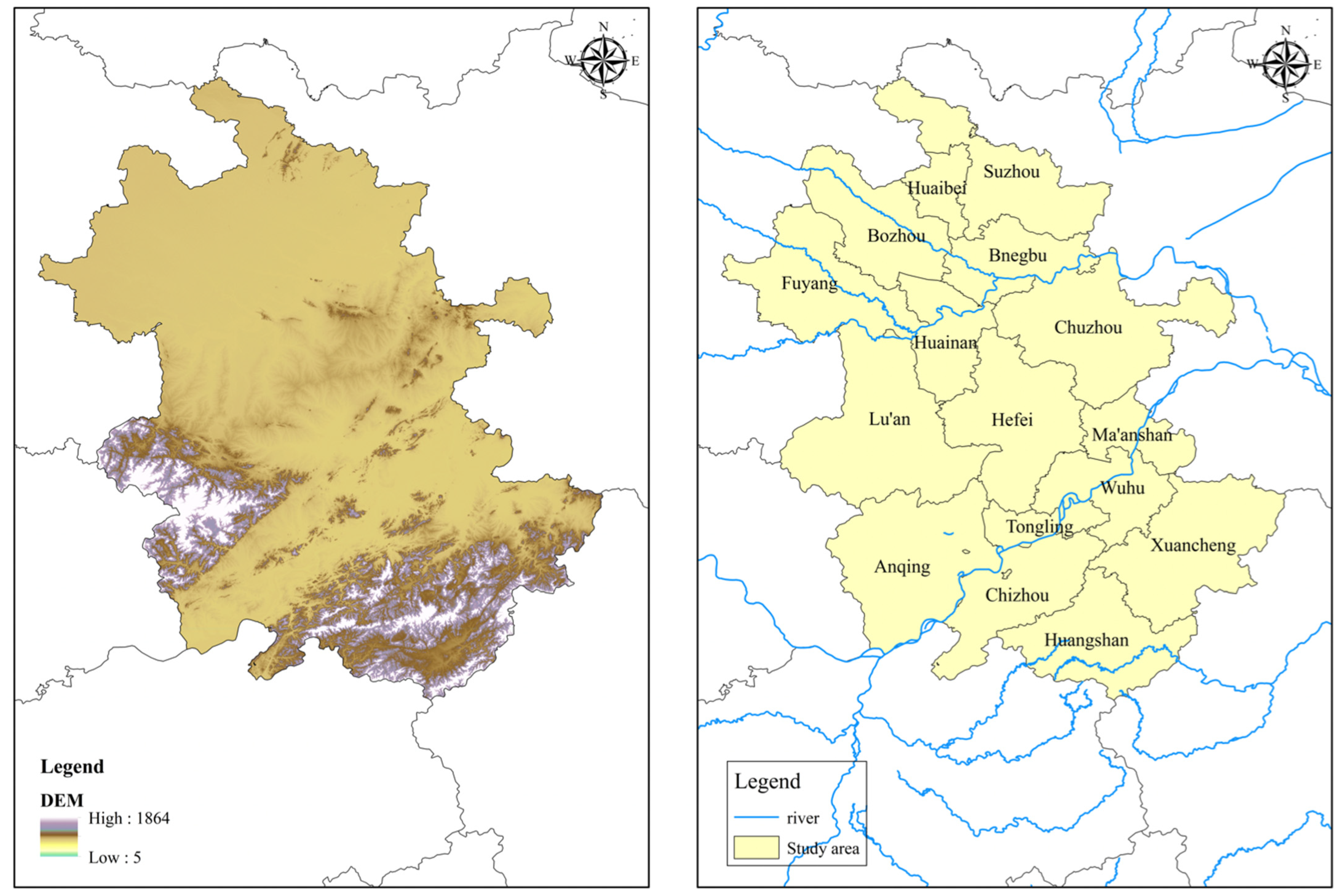
2.1. Study Area

AP is located in the hinterland of Eastern China and encompasses a total area of 140,100 square kilometers (Figure 2). The region’s topography and geomorphology are complex and diverse, comprising five primary geomorphological zones: the Huaihe River Plain, the Jianghuai Terrace Hills, the Western Anhui Hills and Mountains, the Riverine Plain, and the Southern Anhui Hills and Mountains. AP is located between warm temperate and subtropical zones. Specifically, the area north of the Huaihe River is characterized by a warm temperate zone with a semi-humid monsoon climate, whereas the region south of the Huaihe River experiences a subtropical humid monsoon climate. The WRs in AP are notably abundant [41]. The rivers have low sand contents, the flood season is in summer and fall, the rivers have no freezing period, and the main rivers are the Huaihe River, Yangtze River, and Qiantang River. These water systems not only provide ample water for agricultural production but also constitute the unique natural landscape of AP. These rich climatic and topographical features provide an excellent growing environment for many plants and animals; thus, AP is rich in diverse biological resources and maintains a good ecological environment [42]. Within a climatic transition zone, forest vegetation exhibits transitional characteristics. Specifically, the woodland north of the Huaihe River predominantly consists of warm temperate deciduous broad-leaved forests. In contrast, the region south of the Huaihe River is characterized by northern subtropical evergreen and deciduous broad-leaved mixed forests, as well as middle subtropical evergreen broad-leaved forest zones [43].

2.2. Data Sources

The data were obtained from the AP Statistical Yearbook, AP Prefectural Statistical Yearbook, AP WR Bulletin, AP Ecological Environment Condition Bulletin, and AP National Economic and Social Development Statistical Bulletin, and missing data were estimated and fitted via the linear trend method.

2.3. The WR-WECC Evaluation System

In this study, we refer to relevant research results [44,45,46] and combine the natural endowment and development and utilization of WRs in AP with regional hydrological characteristics, pollution pressure, and socio-economic needs. A total of 22 indicators across the three subsystems of WR, socio-economy, and ecology were selected to construct the comprehensive evaluation index system of WR-WECC in AP (

Table 1. WR-WECC evaluation system.

Criterion Layer	Index Layer	Unit	Attribute
WS	X1 Total water resources (Billion)	m3	+
	X2 Water resources per capita	m3/person	+
	X3 Water consumption per capita	m3/person	−
	X4 Precipitation	mm	+
	X5 Modulus of water production	m3/km2	+
	X6 Modulus of water supply	m3/km2	−
	X7 Water resources development	%	+
SS	X8 Population density	person/km2	−
	X9 Natural population growth rate	%	−
	X10 Urbanization level	%	−
	X11 GDP per capita	Yuan	+
	X12 Water consumption of 10,000 Yuan	GDP m3/CNY 10,000	−
	X13 Water consumption of 10,000 Yuan of industrial added value	m3/million Yuan	−
	X14 Irrigation water consumption rate	%	−
	X15 Industrial water consumption rate	%	−
	X16 Tertiary industry	%	+
ES	X17 Ecological water guarantee rate	%	+
	X18 Centralized urban wastewater treatment rate	%	+
	X19 10,000 Yuan of Industrial Output Value COD Emission Intensity	kg/million Yuan	−
	X20 10,000 Yuan GDP Chemical Oxygen Demand Emission Intensity	kg/million Yuan	−
	X21 Forest cover rate	%	+
	X22 Greening coverage rate of built-up area	%	+

). The water resources subsystem primarily encompasses the natural endowment and the development and utilization of water resources. The socio-economic development level directly influences the regional WR-WECC status, while the ecological environment serves as a crucial guarantee for the sustainable utilization of water resources.

The fundamental reason for including ES in the WR-WECC framework is the intrinsic link between ecological conditions and water environment quality. While traditional water environment assessment usually focuses on pollution parameters (e.g., emissions in X19–X20), ecological factors such as forest cover (X21) and green infrastructure (X22) directly affect water conservation, erosion control, and pollutant filtration, thus indirectly regulating the capacity of the water environment. In addition, the ecological water guarantee rate (X17) and sewage treatment rate (X18) are key management indicators linking water utilization and environmental protection. This holistic approach ensures that the evaluation system captures both the direct anthropogenic pressures and the natural ecological processes that maintain the resilience of the water environment.

3. Methods

3.1. Differential Evolution Projection Pursuit Modeling

Differential evolution projection pursuit modeling (DE-PPM) is an advanced method for analyzing high-dimensional data, integrating projection pursuit (PP) and differential evolution (DE) algorithms. The primary objective of this approach is to map high-dimensional data onto a low-dimensional space by optimizing the projection direction. This process aims to uncover the underlying structure within the data while simultaneously leveraging the global search capability of DE to avoid the local optima often encountered with traditional gradient methods [47]. The detailed formula for the DE-PPM [48,49,50,51,52,53] is as follows:

(1)

Data preprocessing

A Box-Cox transformation is applied to the original data matrix $X^{origin}\in R^{n\times p}$ to eliminate nonlinear effects:

$$x_{kj}^{transform}=\left\{\begin{array}{lll}{\displaystyle \frac{{\left(x_{kj}^{origin}\right)}^{\lambda }-1}{\lambda }},\hfill & \lambda \ne 0\hfill & \hfill \\ \ln x_{kj}^{orgin},\hfill & \lambda =0\hfill & \hfill \end{array}\right.$$

(1)

where n is the number of samples, $p$ is the variable dimension, and $\lambda$ is the transformation parameter. where $x_{kj}^{origin}$ is the original value of the $k$th sample, the $j$th feature.

The optimal parameter ${\lambda }^{*}$ is solved via great likelihood estimation:

$${\lambda }^{*}=\arg {\max }_{\lambda }\left[-{\displaystyle \frac{n}{2}}\ln {\widehat{\sigma }}^2(\lambda )+(\lambda -1){\displaystyle \sum _{k=1}^n\ln }{x}_{kj}^{origin}\right]$$

(2)

where ${\widehat{\sigma }}^2(\lambda )$ is the variance of the transformed data.

The data were standardized according to the median ${\tilde{\mu }}_j$ and interquartile range $IQ{R}_j$:

$$\begin{array}{l}{x}_{kj}={\displaystyle \frac{x_{kj}^{\mathrm{transform}}-{\tilde{\mu }}_j}{IQ{R}_j}},\\ \left({\tilde{\mu }}_j=\mathrm{median}\left(\{x_{1j}^{\mathrm{transform}},\dots ,x_{nj}^{\mathrm{transform}}\}\right), IQ{R}_j=Q_3-Q_1\right),\\ Q_1=\mathrm{quantile}(x_{:j}^{\mathrm{transform}},0.25),\\ Q_3=\mathrm{quantile}(x_{:j}^{\mathrm{transform}},0.75)\end{array}$$

(3)

(2)

Parameterization of the projection direction

A spherical coordinate parameterization is first performed to parameterize the unit projection direction vector $a\in R^p$ to the angle $\theta =[{\theta }_1,\dots ,{\theta }_{p-1}]$.

$$\begin{array}{l}{a}_1=\cos {\theta }_1({\theta }_1\in [0,\pi ]),\\ a_2=\sin {\theta }_1\cos {\theta }_2({\theta }_2\in [0,\pi ]),\\ ⋮\\ a_{p-1}=\left({\displaystyle \prod _{k=1}^{p-2}\sin }{\theta }_k\right)\cos {\theta }_{p-1}({\theta }_{p-1}\in [0,2\pi ]),\\ a_p={\displaystyle \prod _{k=1}^{p-1}\sin }{\theta }_k\end{array}$$

(4)

Then, orthogonal projection constraints are applied to multiple projection directions $\{a_1,\dots ,a_m\}$. Generated via Gram–Schmidt orthogonalization:

$$\begin{array}{l}{a}_i^{\top }{a}_j={\delta }_{ij},\\ a_k={\displaystyle \frac{v_k-{\displaystyle \sum _{i=1}^{k-1}(v_k^{\top }{a}_i)}{a}_i}{{‖v_k-{\displaystyle \sum _{i=1}^{k-1}(v_k^{\top }{a}_i)}{a}_i‖}_2}}\end{array}$$

(5)

where $v_k$ is the initial non-orthogonal vector

(3)

Projective indicator function

After the data $z_i=x_i^{\top }a$ are projected, the indicator function is defined as

$$Q(a)=\alpha \cdot \underset{\mathrm{the} \mathrm{density} \mathrm{term} Q_d}{\underbrace{{\displaystyle \frac{1}{n^{2}h}}{\displaystyle \sum _{i=1}^n{\displaystyle \sum _{j=1}^{n}K}}\left({\displaystyle \frac{z_i-z_j}{h}}\right)}}+\beta \cdot \underset{\mathrm{the} \mathrm{entropy} \mathrm{term} Q_e}{\underbrace{\left(-{\displaystyle \sum _{i=1}^n\widehat{f}}(z_i)\ln \widehat{f}(z_i)\right)}}$$

(6)

where $K(u)={\displaystyle \frac{1}{\sqrt{2\pi }}}{e}^{-u^2/2}$ is the Gaussian kernel function, $h=1.06\cdot {\widehat{\sigma }}_z\cdot n^{-1/5}$, $\widehat{f}(z_i)={\displaystyle \frac{1}{nh}}{\displaystyle \sum _{j=1}^{n}K}\left({\displaystyle \frac{z_i-z_j}{h}}\right)$ is the kernel density estimate, and $\alpha ,\beta \in [0,1]$ is the weighting coefficient that satisfies $\alpha +\beta =1$.

To constrain the shape of the distribution, a penalty term $Q_{\mathrm{penalized}}$ is introduced:

$$Q_{\mathrm{penalized}}=Q(a)-{\gamma }_1\left|S(z)\right|-{\gamma }_2\left|K(z)-3\right|$$

(7)

Sample skewness:

$$S(z)={\displaystyle \frac{1}{n}}{\displaystyle \sum _{i=1}^n{\left(\frac{z_i-{\mu }_z}{{\sigma }_z}\right)}^3}$$

(8)

Sample kurtosis:

$$K(z)={\displaystyle \frac{1}{n}}{\displaystyle \sum _{i=1}^n{\left(\frac{z_i-{\mu }_z}{{\sigma }_z}\right)}^4}$$

(9)

where ${\gamma }_1,{\gamma }_2\ge 0$ are the penalization factors.

(4)

Differential evolutionary algorithm

Generate initial population ${\left\{{\theta }_i^{(0)}\right\}}_{i=1}^{NP}$, where $NP$ is the population size

$${\theta }_{i,k}^{(0)}~\left\{\begin{array}{lll}\mathrm{Uniform}(0,\pi ),\hfill & 1\le k\le p-2\hfill & \hfill \\ \mathrm{Uniform}(0,2\pi ),\hfill & k=p-1\hfill & \hfill \end{array}\right.$$

(10)

Next, the scaling factor $F$ and the crossover probability CR are adaptively adjusted with iterations:

$$F^{(g)}=F_{\min }+(F_{\max }-F_{\min })e^{-\eta g/G_{\max }}$$

(11)

where $F_{\min }=0.1$, $F_{\max }=0.9$, $\eta$ is the decay rate, and $G_{\max }$ is the maximum number of generations.

$$C{R}^{(g)}=C{R}_{\mathrm{base}}+{\displaystyle \frac{g}{G_{\max }}}(C{R}_{\max }-C{R}_{\mathrm{base}})$$

(12)

where $C{R}_{\mathrm{base}}=0.2$ and $G_{\max }=0.9$.

For individual ${\theta }_i^{(g)}$, the compilation strategy is chosen with probability $p_{\mathrm{rand}}$:

Formulation of the stochastic mutation strategy:

$$v_i^{(g)}={\theta }_{r1}^{(g)}+F^{(g)}\cdot \left({\theta }_{r2}^{(g)}-{\theta }_{r3}^{(g)}\right)$$

(13)

$\mathrm{r}1,\mathrm{r}2,\mathrm{r}3$ are the indices of three different individuals randomly selected from the population, where $r1\ne r2\ne r3\ne i$. $F^{(g)}$ is the scaling factor for the $g$th generation, usually $F\in (0,2]$.

The optimal individual-based mutation strategy is formulated as follows:

$$v_i^{(g)}={\theta }_{\mathrm{best}}^{(g)}+F^{(g)}\cdot \left({\theta }_{r1}^{(g)}-{\theta }_{r2}^{(g)}\right)$$

(14)

In differential evolutionary algorithms, mutation operations may generate out-of-bounds parameter presets. Boundary reflection processing maps the out-of-bounds parameters back to the feasible domain via symmetric reflection. The formula is as follows:

$$v_{i,k}^{(g)}=\left\{\begin{array}{lll}2{\theta }_{\min }-v_{i,k}^{(g)},\hfill & \mathrm{if} v_{i,k}^{(g)}<{\theta }_{\min }\hfill & ({\theta }_{\min }=0)\hfill \\ 2{\theta }_{\max }-v_{i,k}^{(g)},\hfill & \mathrm{if} v_{i,k}^{(g)}>{\theta }_{\max }\hfill & ({\theta }_{\max }=\pi \mathrm{or} 2\pi )\hfill \\ v_{i,k}^{(g)},\hfill & \mathrm{otherwise}\hfill & \hfill \end{array}\right.$$

(15)

where $v_{i,k}^{(g)}$ is the value of the $k$th parameter for the $i$-th individual in the $g$-th generation. Postvariant values of the $k$ parameters. ${\theta }_{\max }$ is the parameter lower bound, and ${\theta }_{\min }$ is the parameter upper bound.

If $v_{i,k}^{(g)}<{\theta }_{\min }$, it is reflected in the ${\theta }_{\min }$ symmetric position:

$$v_{i,k}^{(g)}\leftarrow 2{\theta }_{\min }-v_{i,k}^{(g)}$$

(16)

If $v_{i,k}^{(g)}>{\theta }_{\max }$, it is reflected in the ${\theta }_{\max }$ symmetric position:

$$v_{i,k}^{(g)}\leftarrow 2{\theta }_{\max }-v_{i,k}^{(g)}$$

(17)

If $v_{i,k}^{(g)}\in [{\theta }_{\min },{\theta }_{\max }]$, no treatment is needed.

Below is the crossover operation used to generate the trial vector. The current individual ${\theta }_i^{(g)}$ and the variation vector $v_i^{(g)}$ are combined to generate the trial vector $u_i^{(g)}$. The formula is as follows:

$$u_{i,k}^{(g)}=\left\{\begin{array}{ll}{v}_{i,k}^{(g)},& \mathrm{if}\mathrm{rand}()\le C{R}^{(g)} \mathrm{or} k=j_{\mathrm{rand}}(j_{\mathrm{rand}}~\{1,2,\dots ,p\})\\ {\theta }_{i,k}^{(g)},\hfill & otherwise\end{array}\right.$$

(18)

where $C{R}^{(g)}\in [0,1]$ is the crossover probability, and where $j_{\mathrm{rand}}$ is randomly selected.

This is followed by a selection operation to update the population. The better solution is retained by comparing the fitness of the test vector $u_i^{(g)}$ to the original individual ${\theta }_i^{(g)}$.

$${\theta }_i^{(g+1)}=\left\{\begin{array}{ll}{u}_i^{(g)},\hfill & \mathrm{if} Q(a_u^{(g)})>Q(a_i^{(g)})\hfill \\ {\theta }_i^{(g)},\hfill & \mathrm{otherwise}\hfill \end{array}\right.$$

(19)

where $Q(a)$ is the projection indicator function used to evaluate the quality of the projection direction a. $a_u^{(g)}$ is the projection direction corresponding to the test vector, and $a_i^{(g)}$ is the projection direction corresponding to the original individual.

(5)

Convergence and stability analysis

The first step is to determine the convergence conditions, which are used to determine when the algorithm stops iterating to ensure that a valid solution is obtained in a reasonable amount of time.

The relative improvement rate threshold $\mathsf{\epsilon }$ is given by

$${\displaystyle \frac{|Q^{(g)}-Q^{(g-1)}|}{\left|Q^{(g-1)}\right|}}<\mathsf{\epsilon }$$

where the algorithm is considered to have converged when the improvement rate is less than $\mathsf{\epsilon }$.

Finally, the Hessian matrix validation is used to verify the stability of the locally optimal solution and to confirm that it is a maximal point. Moments of the second-order derivatives of the objective function Q of the Hessian matrix $H_{kl}$:

$$H_{kl}={\left.{\displaystyle \frac{{\partial }^{2}Q}{\partial {\theta }_k\partial {\theta }_l}}\right|}_{\theta ={\theta }^{*}}(k,l=1,\dots ,p-1)$$

(20)

For $p-1$ dimensional parameter vectors, the Hessian matrix is a symmetric matrix of (p − 1) × (p − 1).

In addition, we need to explain the association of DE-PPM with the assessment of WR-WECC. The DE-PPM method assesses WR-WECC through a three-step process. First, data harmonization is performed. The raw data for the 22 indicators in Table 1 are converted to a harmonized standard format. Second, the importance of each indicator to the water resources carrying capacity is automatically calculated through the optimization algorithm in Equations (10)–(19). Finally, a projected eigenvalue, i.e., a comprehensive score, is finally generated through Equation (20), which directly reflects the degree of harmonization of regional water resources carrying capacity and provides a clear basis for management decisions.

3.2. Obstacle Degree Model

The obstacle degree model (ODM) is used to quantify the degree to which multiple influences impede a goal [54]. The formula for [55,56] is as follows:

(1)

Data standardization

The raw data were normalized so that all indicator values were within the interval [0, 1].

Positive indicators:

$$x_{ij}^{*}={\displaystyle \frac{x_{ij}-\min (x_j)}{\max (x_j)-\min (x_j)}}$$

(21)

Negative indicators:

$$x_{ij}^{*}={\displaystyle \frac{\max (x_j)-x_{ij}}{\max (x_j)-\min (x_j)}}$$

(22)

where X is the original value of the $j$th barrier factor for the $i$th sample. where $\max (x_j)$ and $\min (x_j)$ are the maximum and minimum values of the $j$th factor, respectively.

(2)

Comprehensive obstacle degree calculation

After the projected eigenvalues and normalized values are calculated via the DE-PPM above, the total obstacle degree is calculated for each metric:

$$D_i={\displaystyle \sum _{j=1}^m{w}_j}\cdot x_{ij}^{*}(i=1,2,\dots ,n)$$

(23)

where $D_i$ is the obstacle degree of the $i$th metric, and $w_j$ is the projected eigenvalue.

3.3. Coupling Coordination Degree Model (CCDM)

The coupling coordination degree (CCD) is used to assess the level of synergistic development among multiple systems and comprehensively reflects the interactions among systems and their overall coordination status [57,58].

(1)

Calculation of the Composite Development Index for Systems

$$U_k={\displaystyle \sum _{j=1}^{m_k}{w}_j}\cdot x_{ij}^{*}$$

(24)

where $U_k$ is the composite development index for the kth system. $m_k$ is the number of indicators for the kth system.

(2)

Calculate the degree of coupling

Coupling ($C$) measures the strength of the interaction between systems. It is calculated via the following formula:

$$C=n\times \sqrt[n]{{\displaystyle \frac{U_1\cdot U_2\cdot \cdots \cdot U_n}{{\left(\frac{U_1+U_2+\cdots +U_n}{n}\right)}^n}}}$$

(25)

(3)

Calculation of the degree of coupling coordination

The degree of coupling coordination (V) synthesizes the level of development of the system and the degree of coupling, reflecting the overall state of synergy, and is calculated via the following formula:

$$T={\displaystyle \sum _{k=1}^n{w}_k}{U}_k$$

(26)

$$\mathrm{V}=\sqrt{C\cdot T}$$

(27)

where $T$ is the level of integrated development and V is the degree of harmonization.

3.4. Autoregressive Integrated Moving Average

The autoregressive integrated moving average (ARIMA) model is a time series forecasting method that combines autoregression (AR), differencing (I), and moving average (MA) methods for modeling and forecasting non-stationary time series [59,60]. The general form of ARIMA is $ARIMA(p,d,q)$, where $p$ is the order of AR, $d$ is the number of differences, and $q$ is the order of MA [61].

(1)

Data smoothing

The series is smoothed by eliminating trends and seasonality through differencing [60].

The difference formula is

$${\nabla }^d{Y}_t={(1-B)}^d{Y}_t$$

(28)

where $\nabla$ is a first-order difference operator, d is the number of differences, and $Y_t$ is the observed value of the time series at time t. B is a lag operator satisfying $B^k{Y}_t=Y_{t-k}$.

(2)

Determine the model order (p, q)

Analyzed by plots of the autocorrelation function (ACF) and partial autocorrelation function (PACF). AR(p) is truncated after lag order p for PACF and trailing for ACF. MA(q) is truncated after lag order $q$ for ACF and trailing for PACF. ARMA(p, q) is trailing for both ACF and PACF.

(3)

Parameter estimation

The coefficients $\varphi$ and $\theta$ were estimated via either great likelihood estimation (MLE) or least squares (OLS):

$$\widehat{\varphi },\widehat{\theta }=\arg {\min }_{\varphi ,\theta }{\displaystyle \sum _{t=1}^n{\epsilon }_t^2}$$

(29)

$${\epsilon }_t=Y_t-\left({\displaystyle \sum _{i=1}^p{\varphi }_i}{Y}_{t-i}+{\displaystyle \sum _{j=1}^q{\theta }_j}{\epsilon }_{t-j}\right)$$

(30)

where ${\varphi }_1,\dots ,{\varphi }_p$ is the autoregressive coefficient. ${\theta }_1,\dots ,{\theta }_q$ is the moving average coefficient. ${\epsilon }_t$ is the white noise error term that satisfies a mean of 0, a constant variance, and no autocorrelation.

(4)

Forecasting

Predictions were made via the fitted ARIMA model:

$${\widehat{Y}}_{t+h}={\displaystyle \sum _{i=1}^p{\varphi }_i}{Y}_{t+h-i}+{\displaystyle \sum _{j=1}^q{\theta }_j}{\epsilon }_{t+h-j}+{\epsilon }_{t+h}$$

(31)

Forecast range:

$${\widehat{Y}}_{t+h}\pm z_{\alpha /2}\cdot \sqrt{\mathrm{Var}({\epsilon }_{t+h})}$$

(32)

where $z_{\alpha /2}$ is the quantile of the standard normal distribution.

4. Results

4.1. Horizontal Evaluation of WR-WECC in AP

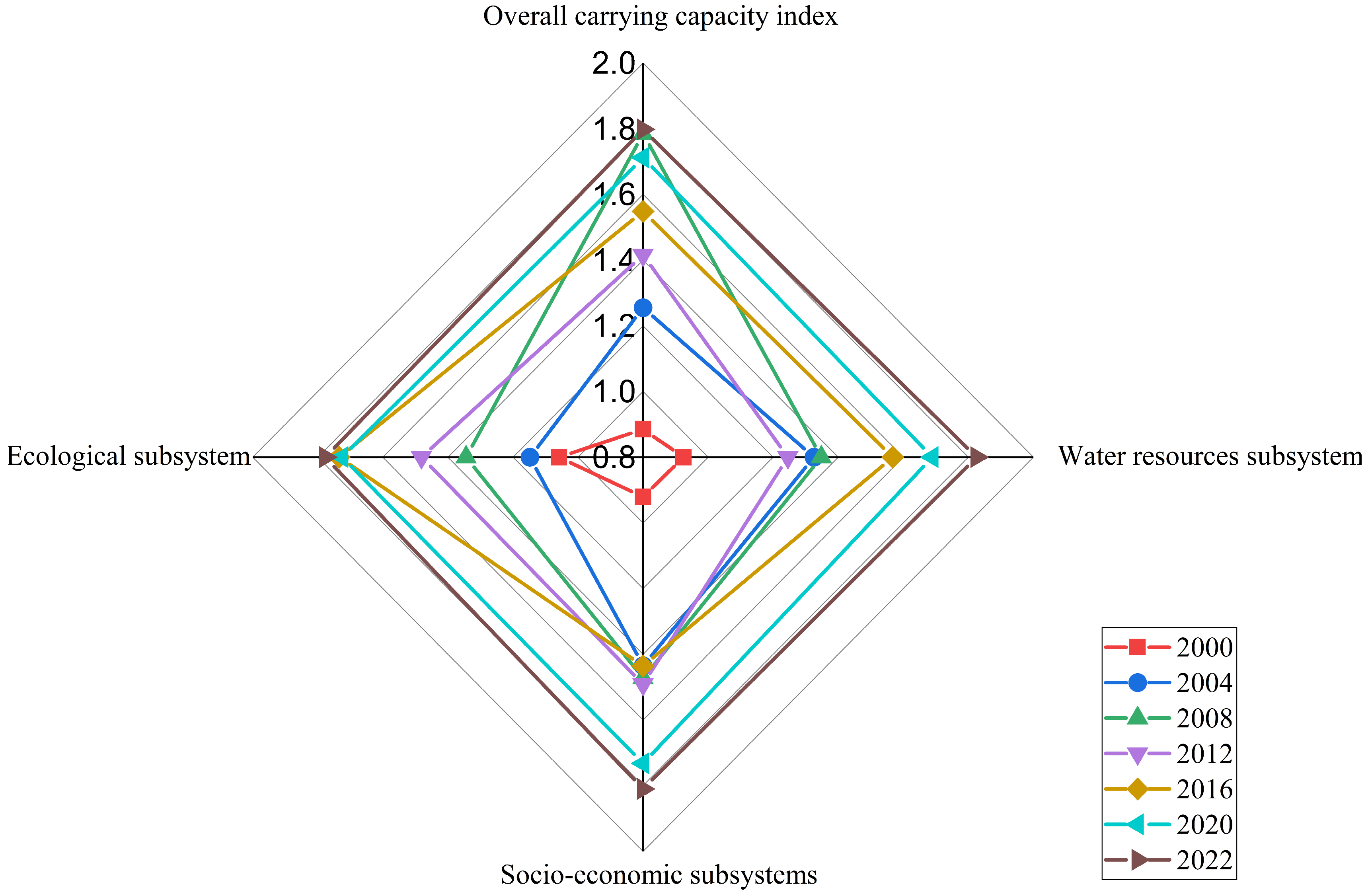
4.1.1. Overall WR-WECC Level Evaluation

On the basis of the DE-PPM, the projected eigenvalues of WR-WECC in AP calculated from 2000 to 2022 were plotted to show the trend of the WR-WECC levels and subsystems, as shown in Figure 3.

Upon analysis of the graph, it is evident that the WR-WECC in AP experienced a significant improvement from 2000 to 2022, with the overall score increasing from 0.885 to 1.798, representing a 103% increase. The WS score rose from 0.924 in 2000 to 1.825 in 2022, with a rapid increase from 2000 to 2007, reaching 1.521, primarily due to early management policies. However, it declined to 1.348 in 2008, before rising again to 1.568 in 2016, attributed to increased precipitation and the implementation of the 13th Five-Year Plan for water conservancy. The rate of increase slowed after 2017, reaching 1.825 in 2022, with the WS lagging behind the SS and ES, thereby negatively impacting the enhancement of WR-WECC in AP. The SS score increased from 0.921 in 2000 to 1.81 in 2022, with a gradual acceleration in growth rate and notable performance post-2019. The socio-economic development level in AP is consistently improving, significantly enhancing water resource utilization efficiency, and the carrying capacity of SS positively influences the enhancement of WR-WECC in AP. The ES score steadily increased from 1.059 in 2000 to 1.777 in 2022, with a stable growth rate from 2000 to 2010, and accelerated post-2016, indicating that AP has effectively managed the ecological environment, achieving significant results.

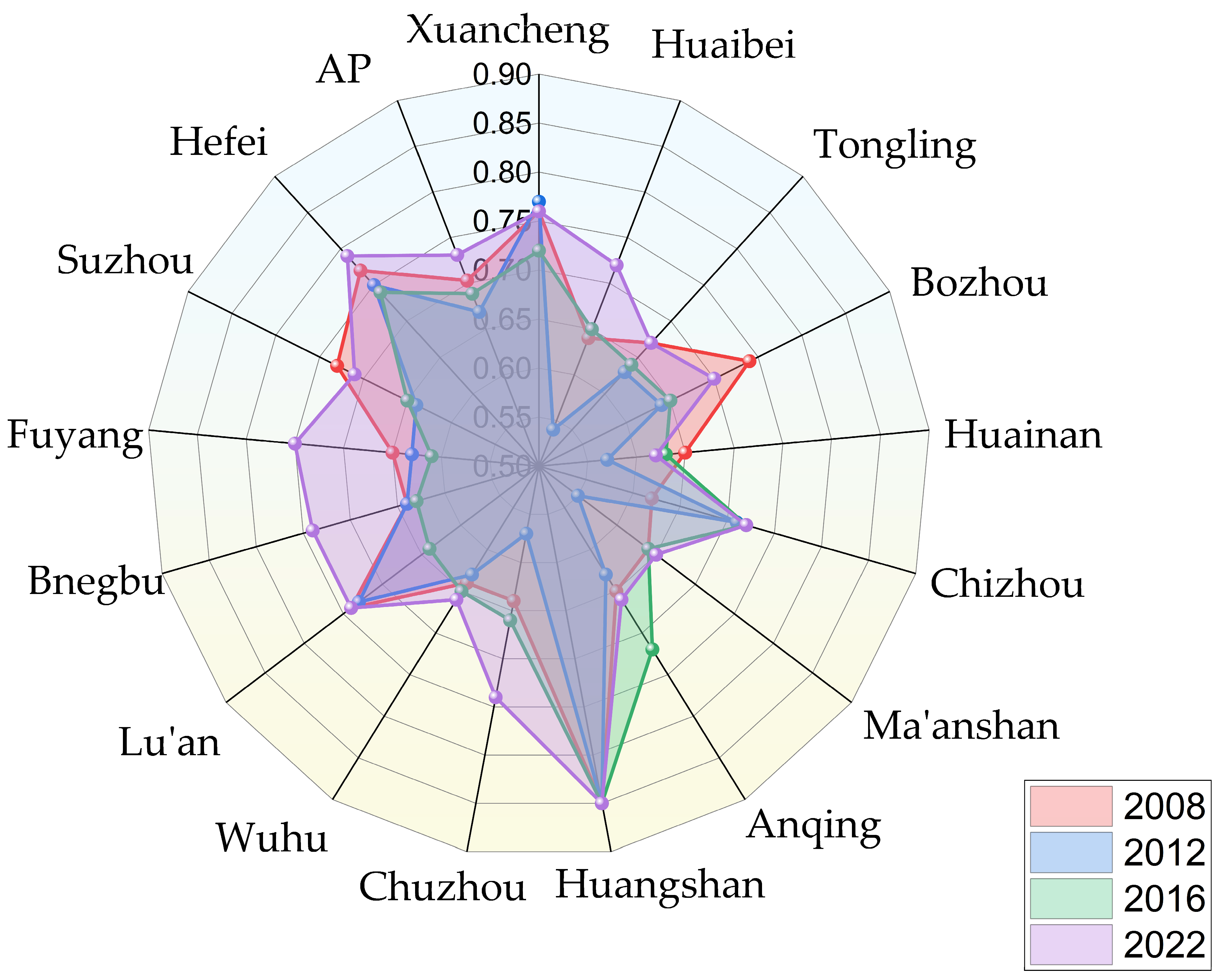
4.1.2. Evaluation of WR-WECC by Municipalities

The projected eigenvalues of the carrying capacity of each municipality were calculated via the DE-PPM, and the spatial visual representation of the projected eigenvalues was carried out via ArcGIS 10.4.1, as shown in Figure 4. With reference to previous studies [62,63], we categorized the load-bearing capacity classes into five levels, namely ideal state (Level I), constrained stage (Level II), weak load-bearing range (Level III), weak non-load-bearing capacity (Level IV), and non-load-bearing interval (Level V).

As shown in Figure 4, the WR-WECC of AP from 2008 to 2022 shows a steady upward trend, rising from the IV weak unloadable stage to the II loadable stage. In 2008, the WR-WECC of AP ranged from [1.217, 1.77], with Huainan being the lowest and Huangshan the highest. Huainan is in the IV weak non-bearing interval. In 2010, the WR-WECC interval of AP was [1.21, 1.886], with Ma’anshan being the lowest and Huangshan the highest. In addition to the IV weak unbearable interval, Fuyang, Bengbu, Chuzhou, and Ma’anshan have dropped from the III weak bearable interval to the IV weak unbearable interval, Huangshan is in the II bearable interval, and the remaining 10 cities are in the III weak bearable interval. In 2012, the WR-WECC interval was [1.285, 1.749], with Huainan at the bottom and Huangshan at the top. Huainan and Ma’anshan were still in the IV weak non-Carrying capacity interval, whereas Chizhou was upgraded to the II carrying capacity interval, and Huangshan was in the I ideal state. The remaining 12 cities had a weak carrying capacity of III. In 2014, the WR-WECC interval was [1.254, 1.894], with Ma’anshan being the smallest and Huangshan the largest. In that year, the WR-WECC values of Hefei, Lu’an, Xuancheng, Chizhou, and Huangshan were within the II-level bearable range, whereas those of the remaining 11 cities were within the III-level weak bearable range. No city was in the IV-level weak, unbearable range. In 2016, the WR-WECC interval was [1.289, 1.798], with Huainan being the smallest and Huangshan the largest. In 2018, the WR-WECC interval was [1.255, 1.757], with Huainan being the smallest and Huangshan the largest. Regional differences are gradually decreasing, with Xuancheng and Huangshan being in an ideal state of Class I, and Huainan and Tongling being worse in Class IV, with weak non-carrying capacity. In 2020, the WR-WECC interval was [1.317, 1.765], with Huainan having the lowest value and Huangshan having the highest value. Fuyang has been downgraded to IV, weak and unloadable, and Ma’anshan has been downgraded to III, weak loadable. In 2022, the WR-WECC interval is [1.317, 1.765], with Huainan having the lowest value and Huangshan having the highest value. Fuyang and Tongling are in the III, weak loadable, interval.

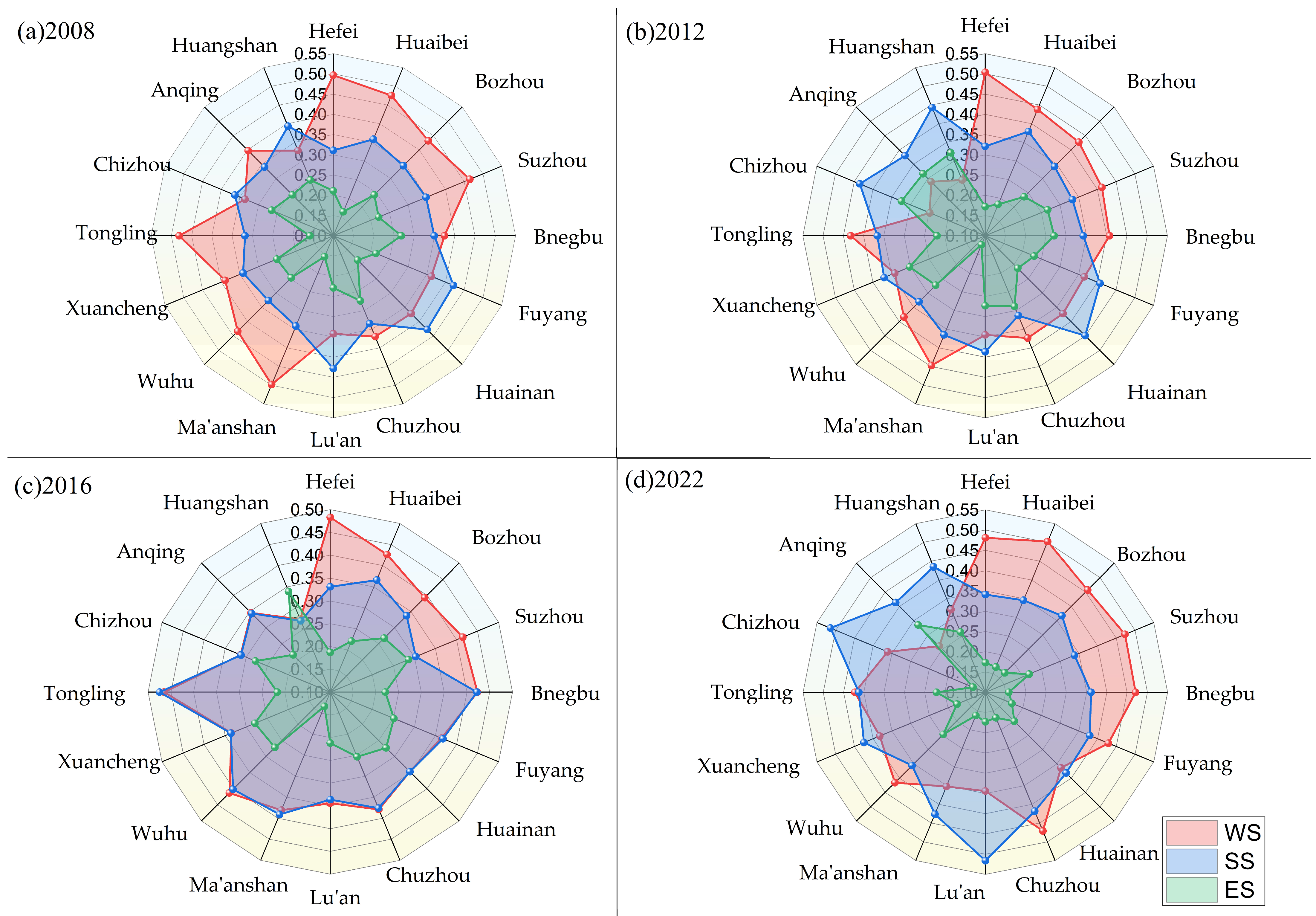
4.1.3. Carrying Capacity Analyses of WS by Municipality

The projected eigenvalues of the carrying capacity of the WS for each municipality were calculated via the DE-PPM, and the results of the evaluation were spatially visualized and expressed via ArcGIS 10.4.2, as shown in Figure 5.

According to Figure 5, the carrying capacity of the WS in each city shows a fluctuating upward trend in the time series from 2008 to 2022. In 2008, the carrying capacity index of the WS in each city in AP ranged from [1.05, 1.884], with the lowest in Suzhou and the highest in Huangshan. Hefei, Huaibei, Suzhou, Huainan, Wuhu, Maanshan and Tongling are at the stage of IV weakly unsupportable WS, Huangshan has reached the ideal state of I, and the other eight cities are at the stage of III weakly supportive WS, which shows that there is a large gap in the WS of the various cities in AP. In 2010, the WS index of the municipalities ranged from [1.14, 1.822]. Suzhou had the lowest value, and Huangshan had the highest value. Wuhu has the lowest value, and Huangshan has the highest value. In 2012, the WS index range of the cities in [1.074, 1.837], Huaibei, Suzhou, Bozhou, Bengbu, and Ma’anshan in the northern Anhui WS carrying capacity in the province, at the end of the range, Huangshan, had the highest index of the carrying capacity of the highest. In 2014, the WS index range of the cities was [1.098, 1.841]; that of Ma’anshan was the lowest, and that of Huangshan was the highest index of the carrying capacity of the subsystem. Tongling had the lowest value, and Huangshan had the highest value. The carrying capacity of Northern Anhui is still poor, and the carrying capacity of Lu’an and Anqing in CA is relatively good, belonging to the class II carrying interval; the carrying capacity of cities in Southern Anhui has a large gap, with Ma’anshan still belonging to the class IV weakly unsupportable interval, Tongling and Wuhu belonging to the class III weakly carrying interval, Chizhou and Xuancheng belonging to the class III weakly carrying interval, and Huangshan belonging to the ideal state of class I. The carrying capacity index of the WS of AP in 2022 ranges from [0.372, 0.802], with Ma’anshan being the lowest and Huangshan being the highest.

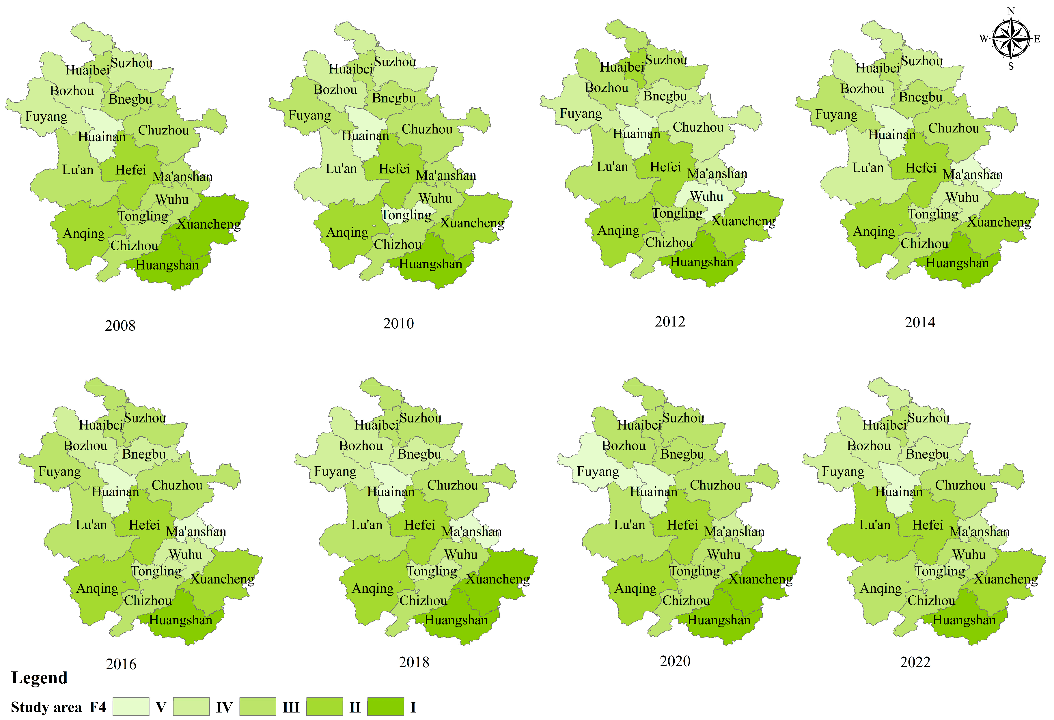
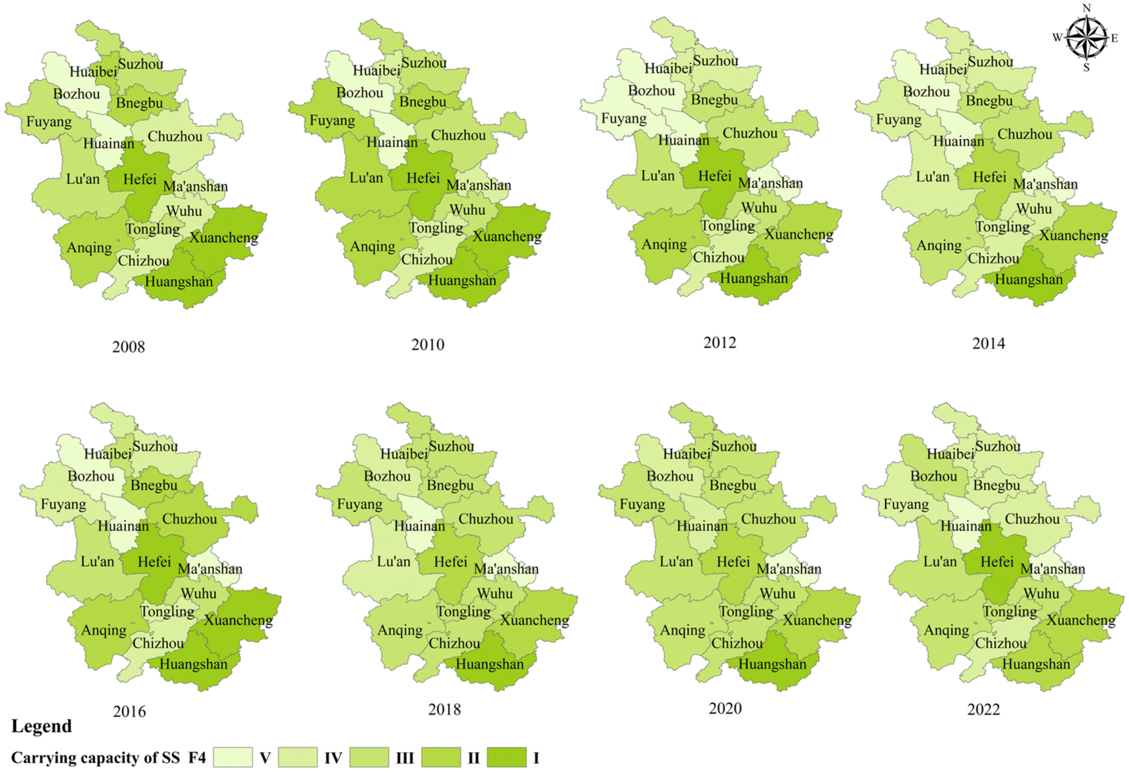
4.1.4. Carrying Capacity Analysis of SS by Municipality

The DE-PPM was applied to calculate the carrying capacity of the SS in each municipality, and the evaluation results were spatially visualized and are expressed in Figure 6.

According to Figure 6, the carrying capacity of the SS of each city in the time series from 2008 to 2022 shows steady growth overall, and the carrying capacity of the SS has a positive pulling effect on the increase in the WR-WESS in AP. In 2008, the range of the SS was [1.414, 1.954], with the lowest value in Ma’anshan and the highest value in Huangshan city. In that year, the SS of the province was only in the weakly unbearable stage of IV in Huainan and in the bearable stage of II in Hefei, Huangshan, and Xuancheng, whereas the remaining 12 cities were in the weakly bearable stage of III. In 2010, the range of the SS was [1.205, 1.997], and it was still the highest in Huangshan and the lowest in Huainan, while the range of the SS was [1.331, 1.825] in 2012. In 2012, the SS ranged from [1.331, 1.825], with the highest value occurring in Hefei, the lowest value occurring in Maanshan, and the composite index of the carrying capacity decreased from 2008 to 2012. The carrying capacity levels of the northern Anhui region, except for Huainan, are all in the weak carrying capacity zone III; the carrying capacity levels of the central and southern Anhui regions are the same as those in 2010, but the composite index is steadily increasing. In 2022, the SS of each city ranged from [1.401, 2.15], with the lowest in Huainan and the highest in Hefei. From 2016 to 2022, the SSs of the six cities in the northern Anhui region exhibited a steady increasing trend, with Huabei showing a steady increasing trend and Hefei showing a decreasing trend. Huaibei city has the highest carrying capacity level, which increases to 0.667 to reach the Class II carrying capacity stage; the carrying capacity of the central Anhui region shows an increasing trend; the carrying capacity levels of the other five cities in the southern Anhui region, except for Ma’anshan city, show a fluctuating downward trend; and Ma’anshan, although the carrying capacity status has improved, is still at the bottom of the province.

4.1.5. Carrying Capacity Analysis of ES by Municipality

The DE-PPM was used to calculate the carrying capacity of the ES in each city, and ArcGIS was used to express the evaluation results via spatial visualization, as shown in Figure 7.

Figure 7 shows that the carrying capacity of the ES of each city from 2008 to 2022 rapidly increased overall. In 2008, the range of ES in each city was [1.185, 2.115], with Chuzhou having the lowest value and Huangshan having the highest value. The carrying capacity of the ES of Bengbu in Northern AP was in the weakly unsupportable interval of class IV, and the other five cities were in the weakly supportable interval of class III; the carrying capacity of the ES of Chuzhou in Central AP was in the weakly unsupportable interval of class IV, and the other three cities were in the weakly supportable interval of class III; the carrying capacity of the ESs of the municipalities in Southern AP varied greatly, with Chizhou being in the weakly unsupportable interval of class IV, Huangshan being in the supportable interval of class II, and the other four cities being in the supportable interval of class III. The carrying capacity of the ES in Southern Anhui varies greatly among cities, with Chizhou at level IV being weakly unsupportable, Huangshan at level II being supportable, and the remaining four cities at level III being weakly supportable.

In 2012, the ESs of the cities ranged from [1.015, 1.95], with Chizhou at the lowest level and Huangshan at the highest level. In the northern Anhui region, the ecological carrying capacity of Suzhou decreased compared with that in 2006; in the central Anhui region, the carrying capacity of Hefei increased to the level II carrying interval, and Anqing decreased to the level IV carrying capacity, which was weakly unsupportable; in the southern Anhui region, the carrying capacity of Wuhu decreased to the level IV carrying capacity, which was weakly unsupportable; during the period of 2008–2012, the carrying capacity indices of the ES of Hefei and Chiuchow only showed a fluctuating upward trend; and the remaining 14 cities showed a fluctuating downward trend, among which Chuzhou showed a decreasing trend, with a decreasing range of [1.015, 1.95]. In 2016, the ES of each city ranged from [1.158, 2.149], with Fuyang being the lowest and Huangshi being the highest. In 2022, the ES of each city ranges from [1.214, 1.866], with Wuhu being the lowest and Xuancheng being the highest, and the ES of the province as a whole increases, with only Anqing being a weakly unsupportable IV and a weakly unsupportable II, with Anqing being a weakly unsupportable II. The carrying capacity of the province as a whole has increased, with only Anqing being weakly unsupportable, and the number of cities in the class II carrying interval increased to 9. Only Tongling and Anqing experienced a decrease in the carrying capacity index of the ES during the period of 2016–2022, whereas the carrying capacity of the remaining 14 cities showed an increasing trend.

4.2. Analysis of the Coupled Coordination of WR-WECC in AP

The DCC of the WR-WECC for the WS-SS-ES system for the years 2008–2022 was obtained via CCDM calculations, and the visual representation of the evaluation results was performed via Origin22, as shown in Figure 8. With reference to previous studies [64], the DCC was classified into 10 levels. When the DCC is between 0 and 0.1, it is grade 1, which corresponds to “extreme dysfunction”; as the DCC increases, the degree of coordination gradually improves, e.g., 0.4 to 0.5 is grade 5, which is “on the verge of dysfunction”, and 0.5 to 0.6 is grade 6, which is “barely coordinated (BC)”. When the DCC reaches 0.6 or above, the coordination state enters a positive development stage, in the order of “primary coordination (PC)” (0.6 to 0.7), “medium-polar coordination (MC)” (0.7 to 0.8), and “good coordination (GC)” (0.8 to 0.9). A DCC value between 0.9 and 1.0 indicates the “quality coordination (QC)” level.

Combined with Figure 8 and

Table 2. Ranking of DCCs in each municipality.

City/Level	2008	2012	2016	2022
Xuancheng	MC	MC	MC	MC
Huaibei	PC	BC	PC	MC
Tongling	PC	PC	PC	PC
Bozhou	MC	PC	PC	MC
Huainan	PC	BC	PC	PC
Chizhou	PC	MC	MC	MC
Ma’anshan	PC	BC	PC	PC
Anqing	PC	PC	MC	PC
Huangshan	GC	GC	GC	GC
Chuzhou	PC	MC	PC	MC
Wuhu	PC	PC	PC	MC
Lu’an	MC	MC	PC	MC
Bnegbu	PC	PC	PC	MC
Fuyang	PC	PC	PC	MC
Suzhou	MC	PC	PC	MC
Hefei	MC	MC	MC	MC
AP	MC	PC	PC	MC

, the range of the DCC in 2008 is [0.62, 0.85], the lowest value is in Chizhou, the highest value is in Huangshan, and the DCC is between level 7 PC and level 9 GC. The 2012 DCC ranges from [0.54, 0.86], with the lowest value in Maanshan and the highest value in Huangshan, and the DCC is between level 6 BC and level 9 GC. The 2016 DCC ranges from [0.61, 0.86]. Fuyang has the lowest value, Huangshan has the highest value, and the coupling coordination is between level 6 BC and level 9 GC. In 2022, the DCC ranges between [0.660, 0.866]. Huainan is the lowest, Huangshan is the highest, and the coupling coordination is between level 7 PC and level 9 GC. Taken together, during the period 2008–2022, the DCC index grew faster and gradually transitioned from level 6 BC to level 9 GC, and the DCC gap between the cities continued to narrow, maintaining between level 7 PC and level 9 GC. The DCC of Southern Anhui is better than that of Northern China and Central Anhui in all years except 2007; Central Anhui is better than that of Northern Anhui in all years except 2007; and NA has the lowest level of DCC in the province in all years except 2007. Compared with Central Anhui, Southern Anhui has a better natural endowment of WRs, better WR support capacity, and relatively earlier socio-economic development, so the DCC level of the carrying capacity system in the SA is relatively high. Therefore, Central Anhui, especially Northern Anhui, needs to take comprehensive measures to improve it, and in the process of socio-economic development, ecological environmental protection investment and governance should be strengthened. The overall DCC of AP shows fluctuating changes with a downward and then upward trend. The coupling level is maintained at PC and MC.

4.3. OD Analysis of WR-WECC in AP

The DE-PPM model was used to evaluate the WR-WECC, and the ODM was used to explore the obstacle factors and the obstacle degree affecting the WR-WECC enhancement. The magnitude of the obstacle factors was judged according to the size of the obstacle degree as a way of analyzing the constraints on the enhancement of the regional WR-WECC.

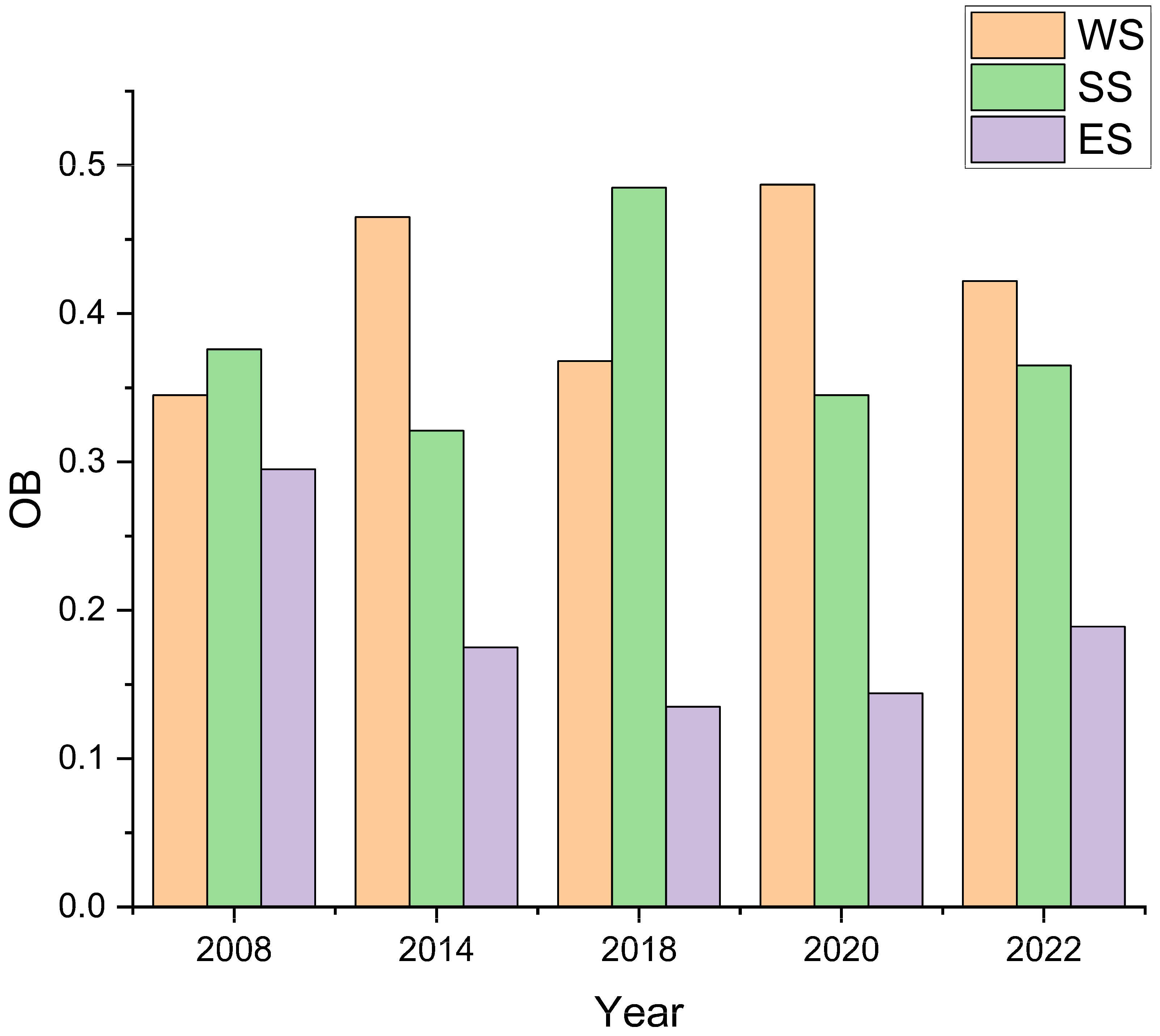
4.3.1. Factor Analysis of Obstacles at the Normative Level

The ODM is used to calculate the obstacle degree of WS, SS, and ES of WR-WECC in AP. To make the results of the guideline layer obstacle degree change more intuitive, the values of the obstacle degree of each guideline layer are plotted as a trend table, as shown in Figure 9.

As shown in Figure 9, the OD values of the three standard layers in 2008 were similar. From 2008 to 2022, the OD value of WS showed a fluctuating upward trend, the OD value of SS fluctuated greatly, and the OD value of ES showed a significant downward trend, but it increased in 2022. Overall, the OD value of ES on WR-WECC enhancement is relatively small, the OD value of WS on WR-WECC enhancement is the largest, and the OD value of SS on WR-WECC enhancement is relatively moderate. WS is the main obstacle affecting the WR-WECC enhancement of AP. The obstacle degree of WS increased from 0.345 to 0.422, indicating that WS is a serious obstacle to the WR-WECC enhancement of AP. This is mainly due to the uneven temporal and spatial distributions of WRs, and the rapid growth of the AP population has led to a substantial increase in water demand. The SS of AP shows a fluctuating trend in the OD index. From 2012 to 2016, the OD of SS decreased from 0.376 to 0.335; from 2016 to 2022, the OD of SS increased from 0.335 to 0.365. The main reason is that large-scale industrial development has led to increases in population and the consumption of resources, which are constrained by water resource conditions and water environment conditions, restricting regional development.

4.3.2. Analysis of WR-WECC Guideline Layer Barrier Factors by Municipality

The ODM was used to calculate the degree of barriers to WS, SS, and ES for each city in the WR-WECC, as shown in Figure 10.

Figure 10 shows that in 2008, the cities of Fuyang, Huainan, Liuan, and Chizhou experienced a relatively high degree of OD of SS, with Liuan exhibiting the most significant constraining effect. The remaining 11 cities were influenced by the constraints of WR-WECC enhancement via WS, with Tongling being the most notably constrained, while the OD of ES was comparatively low. In 2012, Huainan, Liuan, Xuancheng, Chizhou, Anqing, and Huangshan were subjected to a relatively high OD of SS, with Huainan being the most evidently constrained. The other 10 cities were constrained by WS, with Hefei experiencing the greatest constraint, whereas the OD of ES remained relatively low. By 2016, Huainan, Lu’an, Ma’anshan, Xuancheng, Chizhou, Anqing, and Huangshan were significantly constrained by SS, with Lu’an being the most affected. The remaining nine cities were constrained by WS, with Hefei being the most restricted, and the OD of ES continued to be relatively low. In 2022, Hefei, Huaibei, Bozhou, Bengbu, Suzhou, Fuyang, Chuzhou, and Wuhu faced greater barriers from WS, with Huaibei being the most restricted. The other eight cities were subject to the SS, with Chiuchow being the most constrained, and the OD of ES remained low. In the Northern Anhui region, Huainan was constrained by SS, whereas the other five cities were constrained by WS. In the central Anhui region, Lu’an was more evidently constrained by SS, whereas Hefei was primarily constrained by WS. The southern Anhui region experienced an increasingly deeper constraint by SS.

4.3.3. Factor Analysis of Obstacles at the Indicator Level

(1)

Provincial perspective

Through a comprehensive analysis of AP, the ODs of the influencing factors of WR-WECC from 2008 to 2022 were calculated, with the top six factors identified, as presented in

Table 3. Barriers to WR-WECC enhancement for APs.

Year	Obstacle Factor
2008	X5	X21	X12	X19	X1	X2
	12.75	10.15	9.48	8.45	8.32	7.15
2012	X6	X16	X3	X14	X21	X11
	15.62	14.25	12.26	9.15	8.81	7.97
2016	X16	X5	X6	X1	X2	X3
	12.27	10.02	9.74	9.22	8.46	7.72
2020	X6	X8	X5	X9	X10	X3
	13.35	11.24	10.87	9.15	8.3	7.19
2022	X7	X8	X10	X6	X17	X3
	15.66	14.15	13.77	11.33	9.41	8.89

. During the period from 2008 to 2012, AP was influenced primarily by the water supply modulus indicator. In the subsequent period from 2012 to 2016, the water supply modulus continued to be a significant factor, although the obstacles related to the water production modulus intensified. By 2022, the enhancement of WR-WECC in AP was constrained by the WR development and utilization rate, population density, and urbanization level. Analyzing the OD of each indicator reveals that the water supply modulus, water production modulus, proportion of tertiary industry, per capita water consumption, total WR, and forest cover are the principal obstacles to the improvement of the WR-WECC in AP. Among these factors, the water supply modulus, water production modulus, and proportion of tertiary industry are the top three factors impeding WR-WECC improvement in AP. Furthermore, the economic development of APs is driven predominantly by the tertiary industry, which has a substantial demand for WRs, thereby posing significant challenges to the rational development and utilization of WRs and the management of the water environment.

(2)

Municipal perspective

Using the ODM, the OD of the indicator layer for each city in AP was calculated and analyzed, with the top six factors for each city in 2022 identified, as presented in

Table 4. Main barrier factors for WR-WECC from a municipal perspective.

City	Obstacle Factor
Huaibei	X5	X1	X2	X21	X4	X16
	13.44	10.15	9.48	8.45	8.32	7.15
Bozhou	X5	X2	X21	X1	X9	X11
	13.25	12.04	11.24	10.14	9.27	9.11
Suzhou	X5	X2	X1	X21	X16	X11
	12.27	10.02	9.74	9.54	9.41	8.84
Bengbu	X5	X2	X21	X1	X16	X14
	14.41	13.84	12.91	11.04	10.22	9.19
Fuyang	X5	X2	X21	X1	X16	X11
	13.27	12.17	10.75	9.24	9.1	8.47
Huainan	X21	X5	X12	X2	X1	X22
	12.74	11.4	10.26	9.81	9.23	8.61
Chuzhou	X16	X5	X2	X14	X21	X1
	12.02	11.44	11.2	10.26	9.76	9.24
Hefei	X2	X5	X21	X10	X9	X1
	13.52	12.19	11.16	10.54	9.84	9.24
Anqing	X19	X16	X7	X21	X2	X12
	11.05	10.74	10.64	9.84	9.26	8.89
Lu’an	X12	X14	X7	X16	X11	X2
	12.46	12.1	11.72	11.2	10.43	10.12
Ma’anshan	X6	X21	X3	X2	X12	X16
	12.47	11.61	11.4	10.54	10.11	9.77
Wuhu	X21	X2	X16	X12	X15	X3
	11.25	11.01	10.64	10.02	9.24	9.1
Xuancheng	X16	X7	X14	X5	X2	X12
	13.29	12.14	11.29	10.73	9.46	9.01
Tongling	X21	X12	X2	X16	X13	X1
	11.13	10.46	10.29	9.74	9.53	8.77
Chizhou	X16	X7	X12	X3	X11	X13
	11.23	10.95	9.7	9.26	9.11	8.49
Huangshan	X7	X13	X14	X18	X11	X10
	13.56	13.24	12.04	11.46	10.21	9.54

.

In the six cities within Northern Anhui, the primary indicators constraining the enhancement of WR-WECC include the modulus of water production, per capita WR, forest cover, total WR, the proportion of the tertiary industry, and per capita GDP. Notably, the modulus of water production, per capita WR, and forest cover are the three most significant obstacles, with their impacts intensifying. In the four cities in Central Anhui, the main indicators limiting the advancement of WR-WECC are the modulus of water production, per capita WR, forest coverage, the WR development and utilization rate, the proportion of the tertiary industry, and the rate of irrigated agricultural water use. Among these factors, the modulus of water production, per capita WR, and forest coverage rate are the top three obstacles. In the six cities in Southern Anhui, the WR development rate, proportion of the tertiary industry, forest coverage, water consumption per 10,000 yuan of industrial added value, water consumption per capita, and water consumption rate for farmland irrigation are the principal factors impeding the improvement of the WR-WECC. Among these factors, the WR development rate, proportion of the tertiary industry, and forest coverage rate are the top three obstacles.

4.4. Forecast of WR-WECC Levels in AP

The ARIMA model was used to predict the value of change in WR-WECC levels for AP (

Table 5. Forecast of WR-WECC levels in AP, 2025–2040.

Year	True Value	Predicted Value	Residual Value
2000	0.885	0.897	−0.012
2003	1.314	1.113	0.201
2006	1.350	1.343	0.007
2009	1.349	1.680	−0.331
2012	1.415	1.475	−0.059
2015	1.429	1.483	−0.054
2018	1.432	1.553	−0.121
2021	1.736	1.666	0.070
2022	1.798	1.770	0.028
2025		1.890
2028		2.016
2031		2.127
2034		2.247
2037		2.361
2040		2.479

). Most of the residual values were within ±0.2, indicating a good model fit. According to the prediction results from 2025 to 2040, the predicted values increased annually, indicating that the WR-WECC level of AP may show a continuous increasing trend in the future.

The ARIMA model is used to predict the WS level in AP, as shown in

Table 6. Forecast of WS levels in AP, 2025–2040.

Year	True Value	Predicted Value	Residual Value
2000	0.924	0.923	0.001
2003	1.284	1.265	0.019
2006	1.414	1.427	−0.013
2009	1.246	1.418	−0.172
2012	1.245	1.215	0.030
2015	1.338	1.322	0.016
2018	1.348	1.457	−0.109
2021	1.743	1.623	0.120
2022	1.825	1.914	−0.089
2025		1.851
2028		2.026
2031		2.099
2034		2.249
2037		2.340
2040		2.476

. The RMSE was 0.1341, indicating that the predictive accuracy of the model was within the acceptable range. The predicted values increased annually, indicating that the level of WS in AP may continue to increase in the future.

The ARIMA model was used to predict the WS level in AP, as shown in

Table 7. Forecast of SS levels in AP, 2025–2040.

Year	True Value	Predicted Value	Residual Value
2000	0.921	0.959	−0.038
2003	1.330	1.454	−0.124
2006	1.429	1.407	0.022
2009	1.433	1.485	−0.052
2012	1.491	1.594	−0.103
2015	1.452	1.463	−0.011
2018	1.521	1.625	−0.104
2021	1.784	1.820	−0.036
2022	1.810	1.820	−0.010
2025		1.879
2028		1.994
2031		2.108
2034		2.223
2037		2.338
2040		2.453

. The RMSE was 0.1341, indicating that the predictive accuracy of the model was within the acceptable range. The predicted values increased annually, indicating that the level of WS in AP may continue to increase in the future.

The ARIMA model was used to predict the ES level in AP, as shown in

Table 8. Forecast of ES levels in AP, 2025–2040.

Year	True Value	Predicted Value	Residual Value
2000	1.059	1.092	−0.033
2003	1.141	1.188	−0.047
2006	1.182	1.264	−0.082
2009	1.405	1.424	−0.019
2012	1.481	1.523	−0.042
2015	1.643	1.645	−0.002
2018	1.712	1.736	−0.024
2021	1.748	1.807	−0.059
2022	1.777	1.807	−0.030
2025		1.923
2028		2.025
2031		2.125
2034		2.224
2037		2.324
2040		2.424

. The RMSE was 0.0759, indicating that the model had a high prediction accuracy. The prediction results from 2025 to 2040 indicate that the predicted values increase annually, indicating that the level of ES in AP may show a continuous increasing trend in the future.

5. Discussion

This study investigates the spatio-temporal evolution characteristics, influencing factors, coupling relationships, and predictions of the WR-WECC of AP from 2008 to 2022. The study revealed that the WR-WECC of AP showed an overall upward trend, as did WS, SS, and ES. The distribution characteristics of the 16 prefecture-level cities are Southern Anhui > Central Anhui > Northern Anhui, but the regional differences gradually decrease. The DCCM shows that the coordinated development level of WRCC-WECC in the whole province has improved from barely coordinated to well coordinated, and the Southern Anhui region is better than the Central and Northern Anhui regions. The ODM reveals that the indicators of the water supply modulus and water production modulus are the main factors restricting the improvement of the WR-WECC. The ARIMA forecast shows that the WR-WECC and its subsystems in AP will maintain a continuous growth trend until 2040, which provides an important scientific basis for the formulation of regional WR management policies.

The steady improvement trend of the WR-WECC found in this study is closely related to the promulgation of ecological and environmental protection policies for AP in recent years and the practice of industrial transformation. For example, the growth rate of ES is the fastest, which is related to the ecological restoration [65,66] and a comprehensive basin management project of the Yangtze River Bank [67,68] promoted by AP. However, unlike the conclusion of “WS-led WRCC changes” in a similar study in the Yellow River Basin by Chen et al. [69], this study revealed that the driving effect of AP WS on WR-WECC was weaker than that of ES and SS, which may be due to the significant improvement in water resource utilization efficiency in recent years, weakening the influence of traditional WR pressure.

This study elucidates three significant aspects pertinent to regional sustainable development. From a theoretical perspective, the application of WSE-DE-PM facilitates a comprehensive evaluation of the WR-WECC, whereas the DCCM elucidates the coordination dynamics between the WRCC and WECC. This approach holds substantial theoretical importance in addressing challenges such as the uneven spatial and temporal distributions of WRs, water resource security, water environment degradation, and sustainable development in APs. Practically, this research offers support for the sustainable utilization of WRs and water environment management in APs, suggesting the enhancement of water resource utilization efficiency through strategic planning and the allocation of existing WRs. At the policy level, three optimizations are proposed. With respect to WS, in response to WR shortages and the suboptimal development and utilization of WRs, the study advocates for enhanced WR management, the implementation of the strictest WR management system, improved WR utilization efficiency, increased public awareness and education on water conservation, and the establishment of a water-saving society. With respect to SS, which addresses the disparity between economic development and WRs, this study suggests strengthening water conservancy projects, leveraging science and technology to advance water-saving technologies, improving water use efficiency, promoting clean production, and facilitating industrial transformation and upgrading to ensure the sustainable development of the social economy. In terms of ES, with respect to issues such as low forest coverage and inadequate protection of the ecological environment, the author recommends measures to enhance ecological environment control and environmental law enforcement, increase forest coverage, and improve the water ecological environment.

Several limitations are present in this study, as outlined below:

(1)

The comprehensiveness of the evaluation system is constrained. Owing to the delayed disclosure of government data, this study was unable to incorporate critical indicators such as the soil erosion control area and water quality compliance rate in the ES assessment, potentially introducing bias in evaluating the ES carrying capacity.

(2)

The research is limited by the spatial scale of the study area. Currently, the study focuses on the 16 prefecture-level cities of AP, which does not adequately capture the variations in water resources and water environment carrying capacity (WR-WECC) across the Yangtze River, Huaihe River, and Xin’an River Basins within AP.

(3)

There is a limited alignment between the forecasted years and policy frameworks. The model projects up to 2040, yet it is not dynamically integrated with specific projects and carbon emission peaking targets outlined in AP’s “14th Five-Year Plan” for water conservancy, which may impact the effectiveness of the forecast results in informing policy interventions.

In light of these limitations, future research should consider the following:

(1)

Developing a comprehensive index system utilizing multi-source data. By integrating multi-source remote sensing and government data platforms, missing indicators such as river and lake health assessments and groundwater overextraction rates can be supplemented, thereby establishing a more precise indicator system for the AP WR-WECC.

(2)

Investigating watershed characteristics. Future studies should expand the study area to include the Yangtze River, Huaihe River, and Xin’an River Basins within AP to analyze the differences in the WR-WECC across these basins, thereby enhancing the assessment of the WR-WECC status in AP.

(3)

Aligning forecasts with policy frameworks. Implementing policies should be responsive to forecast results, thereby increasing the decision-support value of these forecasts.

6. Conclusions

In this study, we construct WSE-DE-PPM, DCCM, ODM, and ARIMA models to conduct a comprehensive analysis of the AP WR-WECC. The principal findings of the research are as follows:

(1)

From 2008 to 2022, the AP WR-WECC exhibited a consistent upward trend, with the three subsystems generally displaying a fluctuating upward trajectory, among which the ecological subsystem experienced the most rapid growth. The WR-WECC across various cities demonstrated an overall fluctuating upward trend, with a narrowing spatial gap.

(2)

The DCC of the WSE system’s carrying capacity also showed a fluctuating upward trend, gradually transitioning from level 6 to level 9. The level of Southern Anhui was greater than that of Central Anhui and Northern Anhui, with a more significant increase. The DCC of Central Anhui surpassed that of Northern Anhui.

(3)

The OD order of the criterion layer of WR-WECC is WS > SS > ES, where the OD of ES generally shows a downward trend, whereas the OD of WS and SS generally shows an upward trend. Northern Anhui is affected mainly by WS, whereas the central Anhui and southern Anhui regions are restricted by SS. At the index level, the water supply modulus, the water production modulus, and the proportion of tertiary industry are the main obstacle factors restricting the improvement of the AP WR-WECC. The water yield modulus, WR per capita, and forest coverage rate were the main factors influencing Northern Anhui. The restriction of Central Anhui was the same as that in Northern Anhui. The factors restricting the utilization rate of WRs, the proportion of the tertiary industry, and the forest coverage rate in the southern Anhui area are as follows.

(4)

The prediction results for 2025–2040 indicate that the WR-WECC level and the three subsystem levels of AP are expected to continue increasing.

References

1. Lu, L.; Lei, Y.; Wu, T.; Chen, K. Evaluating Water Resources Carrying Capacity: The Empirical Analysis of Hubei Province, China 2008–2020. Ecol. Indic. 2022, 144, 109454. [Google Scholar] [CrossRef]
2. Yang, H.; Hu, D.; Xu, H.; Zhong, X. Assessing the Spatiotemporal Variation of NPP and Its Response to Driving Factors in Anhui Province, China. Environ. Sci. Pollut. Res. 2020, 27, 14915–14932. [Google Scholar] [CrossRef]
3. He, L.; Du, Y.; Wu, S.; Zhang, Z. Evaluation of the Agricultural Water Resource Carrying Capacity and Optimization of a Planting-Raising Structure. Agric. Water Manag. 2021, 243, 106456. [Google Scholar] [CrossRef]
4. Alamanos, A.; Mylopoulos, N.; Loukas, A.; Gaitanaros, D. An Integrated Multicriteria Analysis Tool for Evaluating Water Resource Management Strategies. Water 2018, 10, 1795. [Google Scholar] [CrossRef]
5. Gohari, A.; Mirchi, A.; Madani, K. System Dynamics Evaluation of Climate Change Adaptation Strategies for Water Resources Management in Central Iran. Water Resour. Manag. 2017, 31, 1413–1434. [Google Scholar] [CrossRef]
6. Zou, D.; Cong, H. Evaluation and Influencing Factors of China’s Industrial Water Resource Utilization Efficiency from the Perspective of Spatial Effect. Alex. Eng. J. 2021, 60, 173–182. [Google Scholar] [CrossRef]
7. Liu, P.; Lue, S.; Han, Y.; Wang, F.; Tang, L. Comprehensive Evaluation on Water Resources Carrying Capacity Based on Water-Economy-Ecology Concept Framework and EFAST-Cloud Model: A Case Study of Henan Province, China. Ecol. Indic. 2022, 143, 109392. [Google Scholar] [CrossRef]
8. Wang, G.; Xiao, C.; Qi, Z.; Meng, F.; Liang, X. Development Tendency Analysis for the Water Resource Carrying Capacity Based on System Dynamics Model and the Improved Fuzzy Comprehensive Evaluation Method in the Changchun City, China. Ecol. Indic. 2021, 122, 107232. [Google Scholar] [CrossRef]
9. Kang, J.; Zi, X.; Wang, S.; He, L. Evaluation and Optimization of Agricultural Water Resources Carrying Capacity in Haihe River Basin, China. Water 2019, 11, 999. [Google Scholar] [CrossRef]
10. Ren, L.; Gao, J.; Song, S.; Li, Z.; Ni, J. Evaluation of Water Resources Carrying Capacity in Guiyang City. Water 2021, 13, 2155. [Google Scholar] [CrossRef]
11. Wang, Y.; Wang, Y.; Su, X.; Qi, L.; Liu, M. Evaluation of the Comprehensive Carrying Capacity of Interprovincial Water Resources in China and the Spatial Effect. J. Hydrol. 2019, 575, 794–809. [Google Scholar] [CrossRef]
12. Deng, L.; Yin, J.; Tian, J.; Li, Q.; Guo, S. Comprehensive Evaluation of Water Resources Carrying Capacity in the Han River Basin. Water 2021, 13, 249. [Google Scholar] [CrossRef]
13. Zhao, Y.; Wang, Y.; Wang, Y. Comprehensive Evaluation and Influencing Factors of Urban Agglomeration Water Resources Carrying Capacity. J. Clean. Prod. 2021, 288, 125097. [Google Scholar] [CrossRef]
14. Wang, Y.; Cheng, H.; Huang, L. Water Resources Carrying Capacity Evaluation of a Dense City Group: A Comprehensive Water Resources Carrying Capacity Evaluation Model of Wuhan Urban Agglomeration. Urban. Water J. 2018, 15, 615–625. [Google Scholar] [CrossRef]
15. Wu, L.; Su, X.; Ma, X.; Kang, Y.; Jiang, Y. Integrated Modeling Framework for Evaluating and Predicting the Water Resources Carrying Capacity in a Continental River Basin of Northwest China. J. Clean. Prod. 2018, 204, 366–379. [Google Scholar] [CrossRef]
16. Cao, F.; Lu, Y.; Dong, S.; Li, X. Evaluation of Natural Support Capacity of Water Resources Using Principal Component Analysis Method: A Case Study of Fuyang District, China. Appl. Water Sci. 2020, 10, 192. [Google Scholar] [CrossRef]
17. Mohamed, M.M.; El-Shorbagy, W.; Kizhisseri, M.I.; Chowdhury, R.; McDonald, A. Evaluation of Policy Scenarios for Water Resources Planning and Management in an Arid Region. J. Hydrol. Reg. Stud. 2020, 32, 100758. [Google Scholar] [CrossRef]
18. He, L.; Du, X.; Zhao, J.; Chen, H. Exploring the Coupling Coordination Relationship of Water Resources, Socio-Economy and Eco-Environment in China. Sci. Total Environ. 2024, 918, 170705. [Google Scholar] [CrossRef]
19. Wang, A.; Liang, S.; Wang, S. Coupling Coordination Development of Water Resources-Economy-Ecology System in Shanxi Province Based on System Dynamics. Sci. Rep. 2025, 15, 7370. [Google Scholar] [CrossRef]
20. Zhang, Y.; Khan, S.U.; Swallow, B.; Liu, W.; Zhao, M. Coupling Coordination Analysis of China’s Water Resources Utilization Efficiency and Economic Development Level. J. Clean. Prod. 2022, 373, 133874. [Google Scholar] [CrossRef]
21. Xu, L.; Chen, S.S. Coupling Coordination Degree between Social-Economic Development and Water Environment: A Case Study of Taihu Lake Basin, China. Ecol. Indic. 2023, 148, 110118. [Google Scholar] [CrossRef]
22. Bai, S.; Abulizi, A.; Mamitimin, Y.; Wang, J.; Yuan, L.; Zhang, X.; Yu, T.; Akbar, A.; Shen, F. Coordination Analysis and Evaluation of Population, Water Resources, Economy, and Ecosystem Coupling in the Tuha Region of China. Sci. Rep. 2024, 14, 17517. [Google Scholar] [CrossRef] [PubMed]
23. Zhang, K.; Shen, J.; He, R.; Fan, B.; Han, H. Dynamic Analysis of the Coupling Coordination Relationship between Urbanization and Water Resource Security and Its Obstacle Factor. Int. J. Environ. Res. Public Health 2019, 16, 4765. [Google Scholar] [CrossRef] [PubMed]
24. Qiao, R.; Li, H.; Han, H. Spatio-Temporal Coupling Coordination Analysis between Urbanization and Water Resource Carrying Capacity of the Provinces in the Yellow River Basin, China. Water 2021, 13, 376. [Google Scholar] [CrossRef]
25. Zhang, Q.; Li, Y.; Kong, Q.; Huang, H. Coupling Coordination Analysis and Key Factors between Urbanization and Water Resources in Ecologically Fragile Areas: A Case Study of the Yellow River Basin, China. Environ. Sci. Pollut. Res. 2024, 31, 10818–10837. [Google Scholar] [CrossRef]
26. Ma, H.; Chou, N.-T.; Wang, L. Dynamic Coupling Analysis of Urbanization and Water Resource Utilization Systems in China. Sustainability 2016, 8, 1176. [Google Scholar] [CrossRef]
27. Wan, H.; He, G.; Li, B.; Zeng, J.; Cai, Y.; Shen, X.; Yang, Z. Coupling Coordination Relationship between Urbanization and Water Environment in China. J. Clean. Prod. 2024, 472, 143423. [Google Scholar] [CrossRef]
28. Chen, L.; Wang, X.; Lv, M.; Su, J.; Yang, B. Coupling Coordination and Spatial–Temporal Evolution of the Water–Land–Ecology System in the North China Plain. Agriculture 2024, 14, 1636. [Google Scholar] [CrossRef]
29. Lv, C.; Xu, W.; Ling, M.; Wang, S.; Hu, Y. Evaluation of Synergetic Development of Water and Land Resources Based on a Coupling Coordination Degree Model. Water 2023, 15, 1491. [Google Scholar] [CrossRef]
30. Ren, D.; Hu, Z.; Cao, A. Evaluation and Prediction of the Coordination Degree of Coupling Water-Energy-Food-Land Systems in Typical Arid Areas. Sustainability 2024, 16, 6996. [Google Scholar] [CrossRef]
31. Zhang, Q.; Cao, Z.; Wang, Y.; Huang, Y. Carrying Capacity and Coupling Coordination of Water and Land Resources Systems in Arid and Semi-Arid Areas: A Case Study of Yulin City, China. Chin. Geogr. Sci. 2024, 34, 931–950. [Google Scholar] [CrossRef]
32. Zhao, L.; Yu, J.; Song, X.; Niu, Y.; Xie, J.; Zhang, L.; Li, X. Impact of Land-Use Change on Coupling Coordination Degree of Regional Water–Food–Carbon System. Front. Sustain. Food Syst. 2024, 8. [Google Scholar] [CrossRef]
33. Luo, W.; Jiang, Y.; Chen, Y.; Yu, Z. Coupling Coordination and Spatial-Temporal Evolution of Water-Land-Food Nexus: A Case Study of Hebei Province at a County-Level. Land 2023, 12, 595. [Google Scholar] [CrossRef]
34. Cheng, Y.; Wang, J.; Shu, K. The Coupling and Coordination Assessment of Food-Water-Energy Systems in China Based on Sustainable Development Goals. Sustain. Prod. Consum. 2023, 35, 338–348. [Google Scholar] [CrossRef]
35. Zhang, W.; Liu, C.; Li, L.; Jiang, E.; Zhao, H. The Coupling Coordination Degree and Its Driving Factors for Water–Energy–Food Resources in the Yellow River Irrigation Area of Shandong Province. Sustainability 2024, 16, 8473. [Google Scholar] [CrossRef]
36. Han, C.; Han, X.; Ma, B.; Li, D.; Wang, Z.; Hao, Z.; Zhang, X. Research on the Coupling Coordination Relationship and Spatial Equilibrium Measurement of the Water–Energy–Food Nexus System in China. Water 2025, 17, 527. [Google Scholar] [CrossRef]
37. Gao, J.; Xu, J. Research on the Spatiotemporal Characteristics of the Coupling Coordination Relationship of the Energy–Food–Water System in the Xinjiang Subregion. Sustainability 2024, 16, 3491. [Google Scholar] [CrossRef]
38. Fu, N.; Liu, D.; Liu, H.; Pan, B.; Ming, G.; Huang, Q. Evaluation of the Coupled Coordination of the Water–Energy–Food–Ecology System Based on the Sustainable Development Goals in the Upper Han River of China. Agronomy 2024, 14, 706. [Google Scholar] [CrossRef]
39. Gao, X.; Wang, K.; Lo, K.; Wen, R.; Mi, X.; Liu, K.; Huang, X. An Evaluation of Coupling Coordination between Rural Development and Water Environment in Northwestern China. Land 2021, 10, 405. [Google Scholar] [CrossRef]
40. Zhao, J.; Li, M.; Guo, P.; Zhang, C.; Tan, Q. Agricultural Water Productivity Oriented Water Resources Allocation Based on the Coordination of Multiple Factors. Water 2017, 9, 490. [Google Scholar] [CrossRef]
41. Miao, C.; Sun, L.; Yang, L. The Studies of Ecological Environmental Quality Assessment in Anhui Province Based on Ecological Footprint. Ecol. Indic. 2016, 60, 879–883. [Google Scholar] [CrossRef]
42. Han, W.; Chen, D.; Li, H.; Chang, Z.; Chen, J.; Ye, L.; Liu, S.; Wang, Z. Spatiotemporal Variation of NDVI in Anhui Province from 2001 to 2019 and Its Response to Climatic Factors. Forests 2022, 13, 1643. [Google Scholar] [CrossRef]
43. Xi, M.; Xu, Y.; Li, Z.; Hu, R.; Cheng, T.; Zhou, Y.; Tu, D.; Ji, Y.; Xu, X.; Sun, X.; et al. Progress and Challenges of Rice Ratooning Technology in Anhui Province, China. Crop Environ. 2023, 2, 81–86. [Google Scholar] [CrossRef]
44. Ren, B.; Sun, B.; Shi, X.; Zhao, S.; Wang, X. Analysis of the Cooperative Carrying Capacity of Ulan Suhai Lake Based on the Coupled Water Resources–Water Environment–Water Ecology System. Water 2022, 14, 3102. [Google Scholar] [CrossRef]
45. Li, Y.; Zhang, J.; Song, Y. Comprehensive Comparison and Assessment of Three Models Evaluating Water Resource Carrying Capacity in Beijing, China. Ecol. Indic. 2022, 143, 109305. [Google Scholar] [CrossRef]
46. Kong, Y.; He, W.; Gao, X.; Yuan, L.; Peng, Q.; Li, S.; Zhang, Z.; Degefu, D.M. Dynamic Assessment and Influencing Factors Analysis of Water Environmental Carrying Capacity in the Yangtze River Economic Belt, China. Ecol. Indic. 2022, 142, 109214. [Google Scholar] [CrossRef]
47. Su, Y.; Xu, X.; Dai, M.; Hu, Y.; Li, Q.; Shu, S. A Comprehensive Evaluation of Water Resource Carrying Capacity Based on the Optimized Projection Pursuit Regression Model: A Case Study from China. Water 2024, 16, 2650. [Google Scholar] [CrossRef]
48. Deng, W.; Shang, S.; Cai, X.; Zhao, H.; Song, Y.; Xu, J. An Improved Differential Evolution Algorithm and Its Application in Optimization Problem. Soft Comput. 2021, 25, 5277–5298. [Google Scholar] [CrossRef]
49. Xia, X.; Gui, L.; Zhang, Y.; Xu, X.; Yu, F.; Wu, H.; Wei, B.; He, G.; Li, Y.; Li, K. A Fitness-Based Adaptive Differential Evolution Algorithm. Inf. Sci. 2021, 549, 116–141. [Google Scholar] [CrossRef]
50. Yildizdan, G.; Baykan, Ö.K. A Novel Modified Bat Algorithm Hybridizing by Differential Evolution Algorithm. Expert. Syst. Appl. 2020, 141, 112949. [Google Scholar] [CrossRef]
51. Su, Y.; Liu, Y.; Zhou, Y.; Liu, J. Research on the Coupling and Coordination of Land Ecological Security and High-Quality Agricultural Development in the Han River Basin. Land 2024, 13, 1666. [Google Scholar] [CrossRef]
52. Liu, Z.; Liu, M. Quality Evaluation of Enterprise Environmental Accounting Information Disclosure Based on Projection Pursuit Model. J. Clean. Prod. 2021, 279, 123679. [Google Scholar] [CrossRef]
53. Zhi, G.; Liao, Z.; Tian, W.; Wu, J. Urban Flood Risk Assessment and Analysis with a 3D Visualization Method Coupling the PP-PSO Algorithm and Building Data. J. Environ. Manag. 2020, 268, 110521. [Google Scholar] [CrossRef] [PubMed]
54. Wang, D.; Li, Y.; Yang, X.; Zhang, Z.; Gao, S.; Zhou, Q.; Zhuo, Y.; Wen, X.; Guo, Z. Evaluating Urban Ecological Civilization and Its Obstacle Factors Based on Integrated Model of PSR-EVW-TOPSIS: A Case Study of 13 Cities in Jiangsu Province, China. Ecol. Indic. 2021, 133, 108431. [Google Scholar] [CrossRef]
55. Fan, Y.; Fang, C. Evolution Process and Obstacle Factors of Ecological Security in Western China, a Case Study of Qinghai Province. Ecol. Indic. 2020, 117, 106659. [Google Scholar] [CrossRef]
56. Bai, X.; Jin, J.; Zhou, R.; Wu, C.; Zhou, Y.; Zhang, L.; Cui, Y. Coordination Evaluation and Obstacle Factors Recognition Analysis of Water Resource Spatial Equilibrium System. Environ. Res. 2022, 210, 112913. [Google Scholar] [CrossRef]
57. Dong, Q.; Zhong, K.; Liao, Y.; Xiong, R.; Wang, F.; Pang, M. Coupling Coordination Degree of Environment, Energy, and Economic Growth in Resource-Based Provinces of China. Resour. Policy 2023, 81, 103308. [Google Scholar] [CrossRef]
58. Qi, Y.; Farnoosh, A.; Lin, L.; Liu, H. Coupling Coordination Analysis of China’s Provincial Water-Energy-Food Nexus. Environ. Sci. Pollut. Res. 2022, 29, 23303–23313. [Google Scholar] [CrossRef]
59. Lee, Y.-S.; Tong, L.-I. Forecasting Time Series Using a Methodology Based on Autoregressive Integrated Moving Average and Genetic Programming. Knowl.-Based Syst. 2011, 24, 66–72. [Google Scholar] [CrossRef]
60. Alharbi, F.R.; Csala, D. A Seasonal Autoregressive Integrated Moving Average with Exogenous Factors (SARIMAX) Forecasting Model-Based Time Series Approach. Inventions 2022, 7, 94. [Google Scholar] [CrossRef]
61. Sheikh Khozani, Z.; Barzegari Banadkooki, F.; Ehteram, M.; Najah Ahmed, A.; El-Shafie, A. Combining Autoregressive Integrated Moving Average with Long Short-Term Memory Neural Network and Optimisation Algorithms for Predicting Ground Water Level. J. Clean. Prod. 2022, 348, 131224. [Google Scholar] [CrossRef]
62. Peng, T.; Jin, Z.; Xiao, L. Assessing Carrying Capacity of Regional Water Resources in Karst Areas, Southwest China: A Case Study. Environ. Dev. Sustain. 2023, 25, 15139–15162. [Google Scholar] [CrossRef]
63. Wang, X.; Liu, L.; Zhang, S.; Gao, C. Dynamic Simulation and Comprehensive Evaluation of the Water Resources Carrying Capacity in Guangzhou City, China. Ecol. Indic. 2022, 135, 108528. [Google Scholar] [CrossRef]
64. Gan, L.; Shi, H.; Hu, Y.; Lev, B.; Lan, H. Coupling Coordination Degree for Urbanization City-Industry Integration Level: Sichuan Case. Sustain. Cities Soc. 2020, 58, 102136. [Google Scholar] [CrossRef]
65. Huang, Y.; Li, X.; Liu, D.; Duan, B.; Huang, X.; Chen, S. Evaluation of Vegetation Restoration Effectiveness along the Yangtze River Shoreline and Its Response to Land Use Changes. Sci. Rep. 2024, 14, 7611. [Google Scholar] [CrossRef]
66. Wu, J.; Cheng, S.; Li, Z.; Guo, W.; Zhong, F.; Yin, D. Case Study on Rehabilitation of a Polluted Urban Water Body in Yangtze River Basin. Environ. Sci. Pollut. Res. 2013, 20, 7038–7045. [Google Scholar] [CrossRef]
67. Li, J.; Chen, X.; Zhang, X.; Huang, Z.; Xiao, L.; Huang, L.; Kano, Y.; Sato, T.; Shimatani, Y.; Zhang, C. Fish Biodiversity Conservation and Restoration, Yangtze River Basin, China, Urgently Needs ‘Scientific’ and ‘Ecological’ Action. Water 2020, 12, 3043. [Google Scholar] [CrossRef]
68. Chen, M.; Tan, Y.; Xu, X.; Lin, Y. Identifying Ecological Degradation and Restoration Zone Based on Ecosystem Quality: A Case Study of Yangtze River Delta. Appl. Geogr. 2024, 162, 103149. [Google Scholar] [CrossRef]
69. Chen, Q.; Zhu, M.; Zhang, C.; Zhou, Q. The Driving Effect of Spatial-Temporal Difference of Water Resources Carrying Capacity in the Yellow River Basin. J. Clean. Prod. 2023, 388, 135709. [Google Scholar] [CrossRef]
Figure 1. Technology roadmap.
Water 17 01624 g001
Figure 2. Study area.
Water 17 01624 g002
Figure 3. Trends in WR-WECC and subsystems in AP.
Water 17 01624 g003
Figure 4. Horizontal divergence of WR-WECC by municipality.
Water 17 01624 g004
Figure 5. Differences in the carrying capacity of WS by municipality.
Water 17 01624 g005
Figure 6. Differences in the carrying capacity of SS by municipality.
Water 17 01624 g006
Figure 7. Differences in the carrying capacity of ES by municipality.
Water 17 01624 g007
Figure 8. DCC of WR-WECC in AP.
Water 17 01624 g008
Figure 9. Trends in OB at the guideline level for WR-WECC.
Water 17 01624 g009
Figure 10. AP’s prefecture-level city’s WR-WECC promotion obstacle factor.
Water 17 01624 g010