Abstract
This paper presents a study of the thermal structure, circulation, and mixing processes in an inland water body by taking into account horizontal heterogeneity using a three-dimensional thermohydrodynamics model. The object of this study was the Rybinsk Reservoir, a large inland water body with complex morphology. Field measurement data and ERA5 reanalysis data, as well as a three-dimensional numerical model (which is a development by the authors of this article), were used in this research. The results of the numerical experiments show that three-dimensional numerical modeling, which explicitly takes into account the contribution of seiche oscillations, allows us to describe the temperature distribution in a water body with sufficient accuracy, and this plays a fundamental role in studies of inland water objects. The obtained results could be useful for a model representation of the biochemical processes occurring in lakes and reservoirs. Thus, for models of less spatial detail that are, for example, used to hlrepresent lakes in Earth system models, it is necessary to take into account seiches in the form of parameterizations.
1. Introduction
Lakes and reservoirs cover about 1.3–1.8% of the Earth’s land surface [1,2], and, by now, it has been established that the processes occurring in inland water bodies—and forming such characteristics as the thermal regime, the distribution of concentrations of biochemical substances, heat and gas fluxes into the atmosphere—are of interest both within the framework of hydrology, limnology, and ecology, as well as from the point of view of their influence on the Earth’s climate and its changes [3,4,5].
The temperature regime of water bodies is a defining characteristic of most processes in a water body, and it is related both directly to thermodynamics and to most biochemical cycles [6,7]. Water temperature is important for the production and destruction of organic matter, the gas regime of water bodies, and the dynamics of planktonic and nektonic communities [8]. The temperature of the environment is an important factor influencing the formation of methane since the metabolism of archaea-methanogens (Archaea, Methanoarchaea) directly depends on temperature. The optimal temperature for these microorganisms is 20–42 degrees Celsius [9,10], i.e., higher than the average temperature in lake ecosystems. At the same time, an increase in temperature due to a heating of the surface with subsequent mixing and the formation of a uniform temperature profile across the depth causes an increase in the methanogenesis in bottom sediments. Thus, the type of stratification largely determines the processes of the biochemical cycle in inland waters [11].
One of the physical processes in lakes, which plays a role in mixing, is seiche oscillations—standing gravitational waves that arise due to wind forces, the horizontal transport of mass, and the effect of the hydrostatic pressure gradient in the water body [12]. Seiche oscillations lead to two important effects. First, under the influence of wind, water accumulates on the windward side of the lake, creating a pressure gradient directed against the wind. This gradient generates a compensating current in the epilimnion, which limits the vertical velocity shear and the generation of turbulent kinetic energy, thereby suppressing turbulent transfer and slowing the deepening of the mixed layer. Second, after changes in wind conditions, seiches arise, and their kinetic energy, through an energy cascade, can transform into turbulent kinetic energy, thereby enhancing the vertical effective diffusion of the heat and dissolved substances in the stratified part of the lake. If the horizontal size of the lake exceeds the internal Rossby deformation radius, seiche oscillations become inertia-gravitational, and the Coriolis force begins to play a significant role, contributing to a reduction in the velocity shear with depth and the formation of an Ekman spiral [13], which further reduces mixing. The influence of seiche oscillations on the hydrodynamics and thermal regime of water bodies is often underestimated in existing models, leading to significant errors in reproducing hydrodynamic processes. Global climate models often use a one-dimensional approach to describe horizontally averaged distributions of temperature, momentum, and other characteristics in lakes with depth. One-dimensional models are useful tools to study vertical mixing in lakes but do not account for horizontal effects, such as seiches, limiting their applicability when modeling complex systems.
Currently, there are a number of in situ methods for determining the spatio-temporal variability of various characteristics of aquatic ecosystems, including temperature and stratification. The most common method is hydrological–hydrochemical synchronous surveys, which include field measurements of the thermal characteristics of the reservoir at observation stations. This approach allows for obtaining representative information on the distribution of the studied characteristics in the main sections of the reservoir. However, due to the limited number of observation points, the problem of interpolating the data to sections of the water area not covered by the survey may arise. This can lead to errors in calculating the average values of the studied parameters. The grid of observation stations will always be limited by a set of permanent monitoring stations with homogeneous conditions. If measurements are taken throughout the reservoir, especially if this reservoir is large, it is impossible to obtain the temperature dynamics with a high time resolution, such as, for example, on a daily scale [14]. In addition, hydrological surveys are usually carried out on water bodies several times a year, which complicates the assessment of the temporal dynamics of hydrological characteristics due to the natural variability in synoptic conditions.
The use of three-dimensional numerical models is the only way to obtain a high-resolution spatial distribution of thermal characteristics throughout the entire volume of a water body, especially under conditions of a complex coastline; this heterogeneity cannot be explicitly taken into account in one-dimensional models. Three-dimensional modeling can be used directly to study the thermal regime in conditions of both vertical and horizontal heterogeneity; moreover, it can also be used to calibrate and refine one-dimensional models, which are often used for the parameterization of lakes and reservoirs in global models of the Earth system. Finally, the results of three-dimensional modeling can be applied to planning and preparing measurement campaigns. The configuration of a three-dimensional model describing a specific water body and calibrated using discrete observation data will allow us to obtain the values of characteristics in parts of the reservoir where measurements were not taken, and they will also provide more accurate information about the spatial variability of these characteristics, which must be considered for a competent integral assessment of the parameters of the entire reservoir. In addition, mathematical modeling methods will allow us to solve such problems as assessing the sensitivity of the characteristics being studied to certain parameters of the aquatic ecosystem.
In recent years, several cases are notable in the development of a three-dimensional lake model. Thus, in [15], a three-dimensional Delft3D model was proposed to study a subtropical reservoir. The hydrodynamic module of Delft3D-FLOW [16] solves the Reynolds-averaged Navier–Stokes equations under the assumption of hydrostatic pressure using terrain-matched sigma coordinates. Horizontal spatial discretization is defined on a structured rectangular Arakawa-C grid. Horizontal eddy viscosity is parameterized using the Smagorinsky model assuming a steady state between the turbulent kinetic energy shear production and dissipation. Vertical mixing is described with k- model. Delft3D-FLOW was applied to various natural lakes, such as, for example, the African lake Kivu [17] and the Vietnamese lake Bung Binh Thien [18].
The 3D MIKE 21 and MIKE 3 Flow Model FM (Flexible Mesh) [19] systems are based on the finite volume method applied on an unstructured grid. The Reynolds-averaged Navier–Stokes equations are solved assuming hydrostatic and Boussinesq approximations. The horizontal eddy viscosity is described by the Smagorinsky model, and, for vertical eddy viscosity, the standard k- model is used. The bed resistance is specified as a quadratic drag law. The 3D MIKE 21 and MIKE 3 Flow Model FM have been applied to such water objects as the Baiguishan Reservoir [20] and Douhe Reservoir [21] in China.
The three-dimensional model used in this study is a development on the model constructed by the authors of [22]. It is a part of the unified hydrodynamic code by the Research Computing Center of Moscow State University, and it is based on the combination of DNS-, LES-, and RANS-approaches [22,23,24].
This paper presents a first-of-its-kind study of the Rybinsk Reservoir using both a three-dimensional numerical model and a complex set of in situ measurement data. The purpose of this study was, on the one hand, to create a comprehensive tool designed both for conducting the most detailed studies of water bodies, thereby taking into account the three-dimensional processes, and for verification, calibrating, and refining one-dimensional models, including the most simplified ones used for the parameterization of inland water bodies in Earth system models. On the other hand, within the framework of this work, the authors set the goal of identifying the role of effects associated with three-dimensional circulation in order to develop recommendations for taking them into account when studying the contribution of lakes to global processes, including the formation and change in the Earth’s climate.
The object of this study is an artificial reservoir with a fairly complex internal heterogeneity of temperature. In different parts of the water area in summer, both temperature stratification at the bottom and complete homothermy can be established [25]. In situ measurements of temperature have been actively carried out on the Rybinsk Reservoir [26]: numerous complex field campaigns have been conducted, and profiles of the distribution of water column characteristics, by depth, in different parts of the reservoir have been obtained. The obtained field data were used to develop a three-dimensional model configuration corresponding to the conditions of the Rybinsk Reservoir, as well as to assess the results obtained with the created configuration. The calculation results were compared with measurement data, both with the averaged values for the entire reservoir and those obtained at specific points where observation stations are located. The quality estimates of the model results were also given.
2. The Object of Study
The Rybinsk Reservoir is an artificial reservoir with a valley-type structure to its bed. It is formed by dams on the Volga and Sheksna rivers in the city of Rybinsk. The reservoir’s water area is located within the territories of the Yaroslavl, Tver, and Vologda regions of the Russian Federation. The reservoir body includes a set of flooded river valleys of the Sheksna, Mologa, and Volga (as well as their small tributaries, such as the Suda, Sogozha, Ukhra, and others).
The Rybinsk Reservoir belongs to the Volga-Kama cascade and was filled in 1941–1947. It was created primarily to regulate the flow of the upper Volga basin, as well as for the purpose of generating electricity during Soviet industrialization. The water exchange coefficient was about 1.4 year−1, which classifies the Rybinsk Reservoir as an object with slow water exchange according to the Bogoslovsky classification [27]. The Rybinsk Reservoir is very large in area—4550 km2 at the full supply level of 102 m in the Baltic System. The amplitude of the level during the year can reach 4.9 m; however, this happens quite rarely [28]. Ice formation on the reservoir usually begins in mid-November, and ice cover disappears in mid-April. In the lower part of the reservoir—near the dammed reach of the flooded Sheksna River near the hydroelectric power station—the reservoir does not freeze due to intensive water discharges through the hydroelectric units, and the lower reservoir pool of the hydroelectric complex in Rybinsk also practically does not freeze. Due to the high intensity of biological primary production, the reservoir has a eutrophic status. In summer periods, especially in warm weather conditions, blooming of the water in coastal zones is possible [29]. For the three-dimensional modeling tasks set in this study, a detailed bathymetry map of the Rybinsk Reservoir was created (Figure 1).
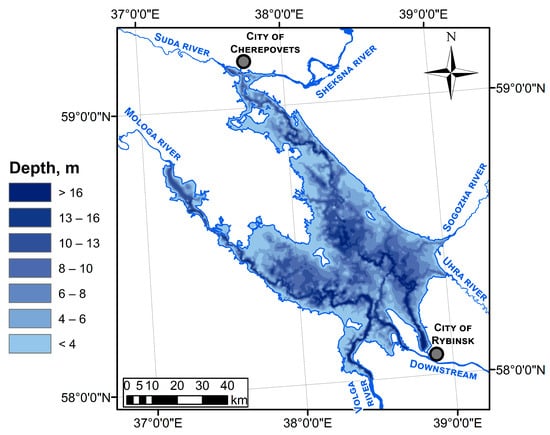
Figure 1.
The bathymetry of the Rybinsk Reservoir.
In the water area of the Rybinsk Reservoir, several characteristic morphometric regions can be distinguished: the Sheksna zone, the Mologa zone (near the dam area), and the Volga tributary zone. The first two regions are flooded river valleys, in which a deeper silted channel trough and shallow floodplain areas stand out, which occupy most of the reservoir. The dam area is the deepest—the greatest depth of the Rybinsk Reservoir (about 30 m) is located there. The Volga tributary zone is distinguished primarily by its hydrological regime, which also stands out a fairly deep channel (up to 20 m), and it also contains floodplain areas and very shallow above-floodplain terraces of the flooded river valley. In general, the Rybinsk Reservoir is a relatively shallow reservoir with complex morphometry.
3. Materials and Methods
3.1. Three-Dimensional Numerical Model of an Inland Water Object
The main research tool, developed at the Research Computing Center of Moscow State University, is a three-dimensional numerical model of an inland water body.
The numerical model includes the equations of hydrodynamics in a stratified turbulent rotating layer of liquid in hydrostatic approximation, as well as an equation for heat transfer that takes into account horizontal and vertical diffusion [24]. The general equations of the model are as follows:
Here, is the velocity vector; f is the Coriolis parameter; T is the temperature; is the density; and are the coefficients of vertical (horizontal) turbulent viscosity and temperature conductivity, respectively; and are the coefficients of molecular viscosity and temperature conductivity, respectively; and z is the vertical coordinate going from the water bottom to the surface. In addition, is the advection operator, and and are the operators defining the horizontal and vertical diffusion with the coefficients and K, respectively.
It should be noted that the model configuration used in this study considers a freshwater body and does not take salinity into account; however, such an option exists and is used, for example, when modeling meromictic lakes.
The numerical method for solving the system of equations is based on conservative finite-difference discretization methods on rectangular grids and the use of a semi-implicit method for time approximation, in which advective transport and horizontal diffusion are described by explicit schemes [23,30].
As for the description of turbulent transport, the model uses two types of closures to calculate the exchange coefficients and . Furthermore, while the model allows using first-order turbulence closures (see, for example, [31]), in this paper, we used the two-parameter (1.5-order) scheme [32]:
Here,
corresponds to the production of TKE due to velocity shear, and
describes the production or consumption of energy due to the action of buoyancy forces. Also, in the given expressions, , are the turbulent Schmidt numbers for the TKE and the dissipation rate, respectively, and and are empirical constants (see, for example, [33]). In the inland water body model, the following values are, in accordance with [23], used: , and is assumed to be equal to for stable stratification and for unstable.
The exchange coefficients are given as follows:
The stability functions and are assumed to be constant in the “standard” scheme, and the values and are used. The model also implements stability functions according to [22,34,35]. In this paper, we took constant stability functions to simplify the analysis. Moreover, the closure with the choice of constants [23] was set to be consistent with the local generalization of the Monin–Obukhov similarity theory.
The temperature profile, which is horizontally uniform for the entire reservoir, was obtained through in situ measurements and was set as the initial condition. The current velocities at the initial moment of time were set to be equal to zero. As for the boundary conditions, on the free surface, the following boundary condition was prescribed:
Here, is the free surface deviation from the equilibrium state. The momentum and heat fluxes were calculated using the Monin–Obukhov similarity theory with Businger–Dyer dimensionless gradients [36,37]. The surface roughness was calculated by Charnock formulae [38]. The logarithmic layer approximation was used to calculate the bottom friction. The flux of penetrating solar radiation was calculated as follows:
where is the surface radiation flux, is the weighting parameter, and and are the extinction coefficients for the longer and the shorter fractions of the shortwave radiation. They can be set constant in accordance with the trophic status of the reservoir (which, in the current study, was m−1 and m−1), or they can be calculated taking into account the correction for the density of chlorophyll-a if the description of the biogeochemical processes in the model is enabled.
On the solid boundaries, the condition of no-penetration was used and the heat flux was set to zero. The reservoir was assumed to be closed, and any inflows or outflows were not taken into account. This assumption was made based on consideration that, although reservoir surface level fluctuations may occur due to flow regulation, their amplitude during the year rarely exceeds 2 m [39]. These changes occur smoothly and affect the thermal structure of the water column much less than the variability of the synoptic situation. Nevertheless, the effect of the water inflow into the reservoir can affect the change in temperature in the zones in the vicinity of rivers, which was taken into account in the analysis of the results and was covered in detail in the comparison of the model results and field measurement data (see Section 4).
The model implementation uses an MPI, OpenMP, and CUDA hybrid approach for performing calculations on parallel computing systems, including heterogeneous ones.
3.2. Field Measurements
The profiles of temperature were obtained during complex hydrological synchronous surveys carried out on the reservoir at 6 stations (Figure 2). The stations are located in the morphometric regions described above (more detailed information on the location of the stations is presented in Table 1).
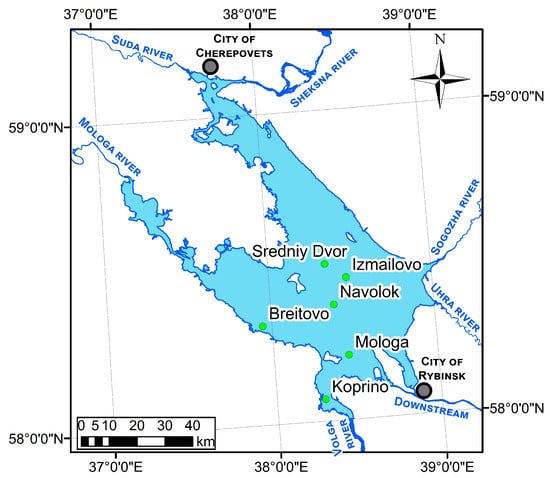
Figure 2.
Observation stations on the Rybinsk Reservoir.

Table 1.
Description of the observation stations on the Rybinsk Reservoir.
At each station, the water column was probed and the temperature was determined at each meter. Series of hydrological measurements have been carried out on the Rybinsk Reservoir since 2010. For the analysis in this study, in situ data for the open water period from May to October in 2013 and 2022 were used. Table 2 shows the dates of the field measurement campaigns that were conducted on the Rybinsk Reservoir during the open water periods in 2013 and 2022.

Table 2.
Dates of the field surveys on the Rybinsk Reservoir in 2013 and 2022.
The most obvious example of the temporal evolution of water temperature can be seen in 2013, the year in which most field campaigns were conducted, thus allowing for the most detailed description of the temporal variability of the studied characteristic to be obtained from discrete field data (Figure 3).
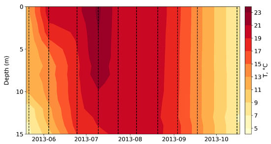
Figure 3.
Temporal distribution of the temperature in the Rybinsk Reservoir averaged for all the measured profiles for 2013. The dotted lines indicate the dates of the field campaigns.
An important feature of the Rybinsk Reservoir is that strongly stable temperature stratification is very rare in it due to wind-induced mixing. Most of the water area of the reservoir is shallow, and the wind influence is very intensive; as such, mixing leads to a relatively uniform temperature distribution by depth. In spring, the reservoir is still slightly warmed up, and its thermal regime is characterized by homothermy. By the beginning of summer, it can be seen that stable stratification establishes the difference between the surface and bottom horizons, which reach about 6 degrees Celsius. Unlike many dimictic reservoirs, during the period of summer heating, the stability of the water column does not increase and the seasonal thermocline is much less pronounced.
Measurement results from 2022 can be briefly described as very similar to the results from 2013 (see Figure 4). The only difference in the temperature stratification regime during the summer period of 2022 is the slightly warmer temperatures in July compared to 2013. The stratification changes from stable to homothermic at the end of August in both years. The differences between the investigated periods are subtle, except for local weather conditions, which vary in different years. The intra-seasonal variations of temperature are much higher than long-term ones.
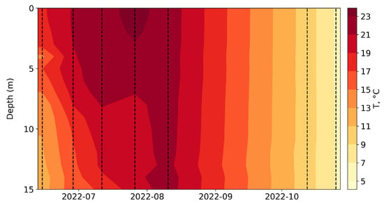
Figure 4.
The temporal distribution of the temperature in the Rybinsk Reservoir averaged for all the measured profiles for the 2022 campaign. The dotted lines indicate the dates of the field campaigns.
However, at individual stations at certain periods of time, the conditions of strongly stable stratification—Figure 5—can be observed.
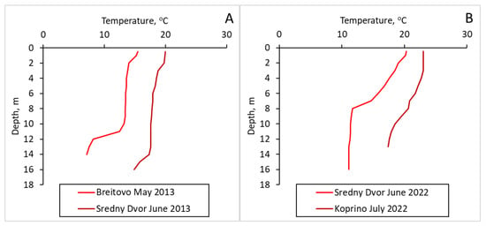
Figure 5.
Stably stratified temperature profiles at individual stations in the Rybinsk Reservoir: (A) 2013 and (B) 2022.
It is possible for stratification to occur in individual parts of the reservoir, while the main part of the water mass is completely mixed, at deep-water stations. These circumstances lead to a high spatio-temporal dispersion of the studied characteristics, which is quite difficult to assess using field observations and, of course, impossible with one-dimensional models. Obtaining sufficiently representative average results for the entire Rybinsk Reservoir using these methods is possible, but, in terms of accuracy, this will be inferior to the results using a full three-dimensional model. This consideration precisely justifies the choice of the main research tool.
3.3. Statistical Metrics
To quantify the modeling results for the temperature stratification in the Rybinsk Reservoir, two statistical metrics were used—root mean square error (RMSE) and RMSE-observations standard deviation ratio (RSR). The formulas for these metrics are as follows:
where corresponds to observational data, to simulation results, is the standard deviation, and is the average value of the observation data.
RMSE is a basic metric for model results quality estimation. In order to standardize obtained RMSE values for model quality categories, it should be normalized on the standard deviation of observation data. Such a method is well known and commonly used in hydrological forecasting and modeling cases [40,41].
4. Numerical Experiments
4.1. Reanalysis Data
The input meteorological parameters in the model are the air temperature, specific humidity, atmospheric pressure, downward fluxes of long-wave and short-wave solar radiation, and the wind speed at surface layer. The ERA5-Land reanalysis [42] was used as the main source of forcing data for the model. During this study, experiments were conducted to assess the impact of forcing data on the model results. In addition to ERA5-Land, numerical experiments with NCEP/NCAR [43] forcing were also conducted. One of the main differences between these data sources was the spatio-temporal resolution, but ERA5-Land had an even finer one at degrees of geographic coordinates and 1 h compared with the degrees and 6 h delivered by NCEP/NCAR. The comparison results showed that a more accurate resolution of meteorological conditions provides a better convergence of the modeled results relative to in situ observations for both shallow-water and deep-water stations throughout the entire open water period (see Figure 6).
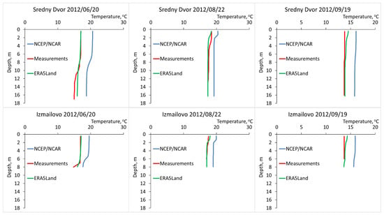
Figure 6.
Comparison of the modeling results with the observational data for the different atmospheric forcing settings using the example of the Sredniy Dvor and Izmailovo station data for 2012.
4.2. Calculations of the Thermal Regime
For the study of the thermal regime of the Rybinsk Reservoir, which involved considering the horizontal heterogeneity, the open water periods of 2013 and 2022 were chosen. These particular periods coincided with thorough measurement campaigns, where a sufficient database of field observations had been accumulated for them for the purposes of comparison and validation of the model (see Table 2). For 2012, the agreement between the measured temperature profiles and those obtained from numerical modeling using the ERA5-Land reanalysis data is shown above in Figure 6.
4.2.1. Temporal Distribution of the Averaged Temperature
We used two model configurations to analyze the temperature distributions during the entire open water period. The first configuration implied the most detailed reproduction of the three-dimensional structure of the Rybinsk Reservoir: the bottom relief was specified, the resolution was 256 points horizontally and 32 points vertically, and the seiches were explicitly taken into account. In the simplified configuration, a formulation corresponding to a one-dimensional one was considered, and the terms responsible for horizontal effects were averaged. The model time of the numerical experiment covered the period from May to November.
Below are the results of the temporal distribution of temperature calculated in the full setup.
Figure 7 and Figure 8 show the simulated temporal evolution of the temperature profiles averaged horizontally over the entire reservoir from May to early November. If we compare them with the measured data (see Figure 3 and Figure 4), we see fairly good agreement, not only quantitatively, but also qualitatively. The model reproduces a typical dimictic cycle with separate phases of stratification and mixing—a common pattern observed in the Rybinsk Reservoir. In May–June, the reservoir transforms from a relatively homothermic state to a more stratified water column. Increased solar radiation and longer daylight hours caused intense heating of the surface waters and the formation of an upper mixed layer. The greatest stability and large gradients were found in July–early August. However, strong wind action led to partial mixing and to the formation of layers of colder water near the surface or a local deepening of the thermocline. This is probably caused by the transfer of water from the lower layers by turbulent eddies or internal seiches. By the end of August and September, the stability of stratification weakened and a clear deepening of the thermocline occurred, ultimately leading to autumn homothermy.
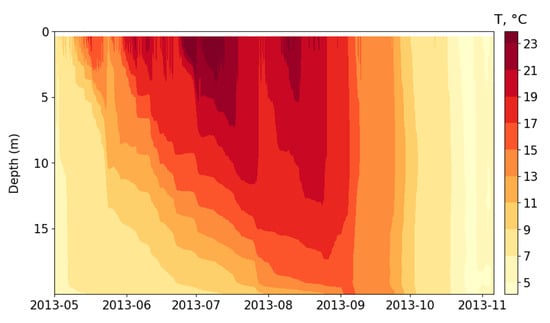
Figure 7.
Temporal distribution of the temperature in the Rybinsk Reservoir, which was obtained in full configuration, for 2013.
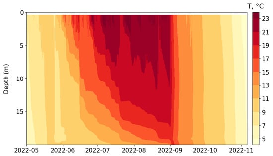
Figure 8.
Temporal distribution of the temperature in the Rybinsk Reservoir, which was obtained in full configuration, for 2022.
To detect the role of processes related to the three-dimensional structure of the reservoir and horizontal transport, a calculation was also performed in a formulation that was close to one-dimensional, where horizontal effects, including seiche oscillations, were averaged. The temperature differences between the full and simplified formulations are given below (Figure 9 and Figure 10).
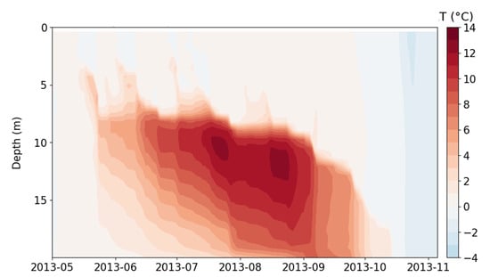
Figure 9.
Temporal distribution of the temperature difference between the full model configuration and the simplified one for the Rybinsk Reservoir, 2013.
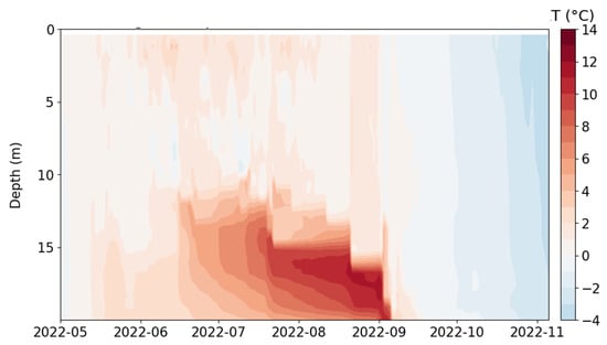
Figure 10.
Temporal distribution of the temperature difference between the full model configuration and the simplified one for the Rybinsk Reservoir, 2022.
For both years under study, a significant difference between the model configurations in the layer below the thermocline (i.e., more than 10 degrees Celsius) under conditions of stable stratification was demonstrated. This is due to the fact that one-dimensional modeling without parameterization of the processes associated with horizontal transport and, in particular, with seiche oscillations, is not able to correctly reproduce mixing processes, thus leading to an underestimation of the epilimnion thickness and errors in temperature distribution. The three-dimensional model also takes into account the vertical “branches” of the circulation cell, the role of which is to transfer the momentum and heat between the upper and lower boundaries of the mixed layer, thereby reproducing mixing of the correct intensity. Note that, despite the general patterns in the results of the numerical experiments, some differences were found for 2013 and 2022, such as, for example, where the disagreement was more pronounced and covered a longer period due to the difference in meteorological conditions in 2013. This was due to the more, in particular, intense wind action inducing the transport processes in the reservoir.
As noted, the three-dimensional model allows for taking into account the bottom bathymetry, the shape of the water body, and mixing dynamics. The complex morphometry of the Rybinsk Reservoir leads to horizontally non-uniform thermal conditions, especially those at great depths, where former river beds and channel depressions are located. Due to these morphometric features, a significant standard deviation of temperature from the average value at each depth horizon can be observed. As shown in Figure 11 and Figure 12, the largest standard deviation from the average value was observed precisely in the bottom horizons, such as, for example, in late summer and early autumn, which is when the reservoir begins to cool and individual deep depressions can retain heat for some time. This is fundamentally important when studying biochemical processes in the inland water body since the temperature regime affects the production of methane by archaea, which occurs in the bottom sediments.
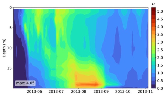
Figure 11.
Temporal distribution of the standard deviation of the temperature from the average value at each depth horizon (obtained within the framework of the three-dimensional modeling of the Rybinsk Reservoir in 2013).
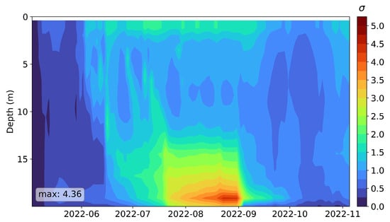
Figure 12.
Temporal distribution of the standard deviation of the temperature from the average value at each depth horizon (obtained within the framework of three-dimensional modeling of the Rybinsk Reservoir in 2022).
4.2.2. Horizontal Heterogeneity at Individual Observation Points
The horizontal heterogeneity was reproduced by the three-dimensional model and was noted both in the temperature distribution and in the current velocity (see Figure 13).
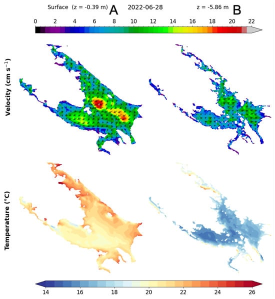
Figure 13.
The temperature and current velocity distribution at the surface (0.39 m) and at 5.86 m depth in the Rybinsk Reservoir (obtained using three-dimensional modeling at a fixed point in time on 28 June 2022).
These figures show an example of the complex circulation of the water masses in the Rybinsk Reservoir that were described earlier. In late June of 2022, the north and northeast winds prevailed over the reservoir, which formed a clockwise rotation of the surface water (Part A of Figure 13). The highest current velocities (up to 20 cm s−1) were observed in the middle part of the reservoir in the open water area. Nevertheless, the northern part of the reservoir remained the most heated. Here, in the upper reaches of the Sheksna and Mologa sections of the water area, heating was more intensive due to the smaller volume of water and shallow depths in this region. In addition, upwelling does not occur in these areas as the depths there are shallower than those in the middle part (Figure 1). The bottom water from the central part cannot flow into these detached areas of the reservoir. The peculiarities of the Rybinsk Reservoir morphometry, in this case, play a determining role in the formation of circulation. In turn, upwelling is observed in the eastern part of the reservoir (Part B of Figure 13). Current velocities at 6 m depth can reach 15 cm s−1. The occurrence of undersurface counter-currents exactly at these water horizons is related to the depth of the thermocline during this period; the largest temperature gradients were observed at 5–6 m depths. The 3D model with explicit morphometry can accurately reproduce the formation of the water mass transport by taking into account local features of the Rybinsk Reservoir, which is impossible to reconstruct, using 1D models with empirical parametrization of horizontal heterogeneity.
To study the horizontal heterogeneity at various points in the Rybinsk Reservoir, three observation stations were selected: Sredniy Dvor, Izmailovo and Koprino. Sredniy Dvor is the deepest station among all of the six measurement points. It was investigated during in situ campaigns, and it is located on the inundated riverbed of the Sheksna river. Izmailovo is a shallow station (with a depth near 8 m), and it is located on floodplain of the Sheksna river basin in the middle of the reservoir. Koprino was selected as a station, and it is located in the most tributaries-affected area—near the zone of the Volga river inflow. These stations represent different conditions in terms of wind mixing and stratification in the Rybinsk Reservoir.
To demonstrate the reproduction of the horizontal heterogeneity by the model, a comparison of numerical results with observation data at specific stations, where measurement campaigns were conducted, was carried out. In addition to the full model configuration, a simplified one corresponding to a one-dimensional model formulation was also considered. Note that the “one-dimensional” model configuration provided only one profile for each date for the entire water body.
As an example of the different stages of the seasonal thermal cycle and the types of temperature stratification, four profiles for each year are shown in Figure 14. From here, the full configuration will be designated as “3D”, and the simplified one, with averaged terms responsible for three-dimensional circulation, will be designated as “1D no seiche”. The profiles demonstrate the following: the beginning of the onset of stratification, stable stratification with the most pronounced gradients, the transition from stratification to homothermy, and late autumn homothermy.
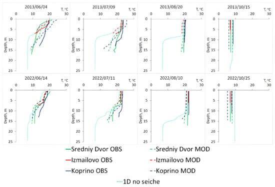
Figure 14.
Temperature profiles at various observation stations for 2013 and 2022 (obtained through in situ measurements and numerical modeling in full and simplified model configurations).
In early June, stratification was established in the reservoir; at the Sredniy Dvor and Izmailovo stations, the epi-, meta-, and hypolimnion were well expressed. At Koprino station, the stratification was weaker due to the Volga inflow impact. Described patterns can be observed both in 2013 and 2022, and the model in full configuration represents temperature profiles correctly. The highest discrepancy between the model and observations appeared for Koprino station because the current model configuration does not take into account the contribution of tributaries and outflows. This is because the reservoir was considered a closed one. However, one should note that the parameterization of the transport of passive tracers (e.g., heat) through the lateral boundary was implemented in the model and was at the testing stage.
In a simplified configuration, the temperature profile for 4 June 2013 demonstrates a much stronger stratification than the observational data show, and this is due to the underestimation of the influence of the wind-wave and seiche mixing observed in the Rybinsk Reservoir that form its thermal structure. The large length of the Rybinsk Reservoir leads to significant wind acceleration on its surface and the occurrence of seiches, which cannot be taken into account in one-dimensional modeling without additional parameterizations.
In mid-July, the underestimation when mixing in the “one-dimensional” model was even more pronounced. In the surface layer, the temperature continued to rise due to summer heating. In the deep layers, the temperature also increased, which was evident from both the results of the observations and calculations with the full three-dimensional configuration. The model also showed very good agreement with the observation data, but the warming in the bottom layer in the simplified configuration proceeded much more slowly.
The temperature regime of the reservoir in August was close to complete homothermy at all measurement stations. A more detailed description of the transformation of the stratification type based on the measurement results is presented in Section 3.2 of this paper. This process was well reproduced in the model (see Figure 7 and Figure 8). Also, good convergence between the full configuration and the observational data can be seen for the profiles of 20 August 2013 and 10 August 2022. The simplified configuration still demonstrated a stratified reservoir with a pronounced metalimnion (temperature gradients of about 8-10 degrees Celsius per meter). This shows the need for further improvement in mixing parameterization in one-dimensional models. The advantage of 3D modeling in this case is that such processes are reproduced explicitly, without empirical parameters, such as the background diffusion coefficient used in one-dimensional models without seiches to solve the problem of underestimation whenmixing.
Complete homothermy was only established in the “one-dimensional” configuration of the model in late autumn, which was evident for the 15 October 2013 and 25 October 2022 profiles. For the 25 October 2022 profile, a stronger heating of the homogeneous profile was noted compared to the in situ data and the full configuration. This may be due to the fact that, in the model configurations, the momentum and heat fluxes are not prescribed but are calculated using the bulk formula based on the Monin–Obukhov similarity theory; as such, the sensible heat flux depends on the difference between the lake surface and atmospheric temperatures. Due to the fact that, in the one-dimensional formulation, higher temperatures were observed during the transition from stable stratification to homothermy, the water body may retain more heat than was observed in the measurement data. The three-dimensional model reproduced the temperature distribution at the Sredniy Dvor and Izmailovo stations quite correctly. The greatest discrepancy in results was at Koprino station due to the inflow–outflow balance, which was described earlier.
4.3. Estimates of the Obtained Results
The metrics described in Section 3.3 were applied to the results obtained in both configurations in comparison with the observation data. The average value of for all available field data was 0.70 and 0.28 for the 1D and 3D configurations, respectively. The RSR value for 1D configuration being equal to 0.70 means that it was a “Satisfactory” result but still very close to “Unsatisfactory”. The RSR value for full 3D configuration being equal to 0.28 means it was “Very Good” result. These values indicate that the 3D model prediction skill of the temperature stratification was close to four times higher than the natural dispersion of temperature in the Rybinsk Reservoir. Table 3 shows more detailed information about the RMSE and RSR values for different observation stations (see Figure 2).

Table 3.
The results of the RMSE and RSR estimations for both model configurations in comparison with the observation data.
The model configuration corresponding to the 1D setup showed “unsatisfactory” results for four of the six observation stations in 2013, and only three of the six stations had “very good” confidence between the configuration and the 2022 observations. The Breitovo, Izmailovo, and Navolok stations are located in the shallow part of the reservoir, where the wind and wave mixing forms a homogeneous temperature profile: for a given depth and weather conditions, it is possible to achieve adequate results, even in the simplified one-dimensional configuration. At the same time, for the conditions of the deepest part of the reservoir, the use of such a configuration can lead to significant uncertainties. This is clearly seen in Figure 14. On the other hand, the full 3D model configuration can describe the water temperature with a “Very Good” performance rating at all stations except Koprino in 2013 (where the RSR value also showed “good” results). The RSR for the Koprino station was also the lowest in 2022. This can be explained by the strong influence of the Volga River tributary, which was discussed above. Thus, statistical estimates confirm the validity of using three-dimensional modeling for such a water object as the Rybinsk Reservoir, which is characterized by high spatial heterogeneity. In the case of one-dimensional modeling, which does not require any substantial computational resources and may be used as lake and reservoir parameterizations in Earth system models, it is necessary to implement parameterizations that allow for the contribution of seiches to mixing.
5. Discussion and Conclusions
In this paper, we present the results of a study of the temperature regime and horizontal heterogeneity in the Rybinsk Reservoir during the open water period using a three-dimensional numerical model. The temperature distribution in an inland water body is an important characteristic related both directly to thermodynamics and to most biochemical cycles. The research tool discussed in this paper is a numerical model of an inland water body, within the framework of which a configuration corresponding to the conditions of the Rybinsk Reservoir was developed. The features of the model proposed by the authors are a mixing scheme consistent with the Monin–Obukhov similarity theory, finite-difference conservative approximations, and an efficient parallel implementation for use on supercomputers that can conduct high-resolution simulations.
The model explicitly takes into account the processes associated with three-dimensional circulation, including seiche dynamics. Seiches are caused by the horizontal redistribution of the mass and the effect of the hydrostatic pressure gradient; they are not incorporated into the majority of the existing one-dimensional (vertical) models. At the same time, seiche oscillations significantly affect the formation of the thermal structure of the water body. To investigate the role of seiches, a series of numerical experiments was conducted in two configurations created within the framework of this study. The full configuration implied the most detailed description of the structure of the Rybinsk Reservoir with the bottom bathymetry, and seiches were explicitly taken into account. In the simplified configuration, a formulation corresponding to a one-dimensional model was considered, and the terms in the governing equations were averaged in horizontal directions.
The Rybinsk Reservoir is an artificial reservoir with a valley-type structure to its bed. The data from the conducted field measurements were used both as the input for the model (initial temperature profile) and for comparison with the model results—both the average temperature values for the entire reservoir and the profiles were obtained at individual observation stations. For the analysis in this study, in situ data for the open water period from May to October in 2013 and 2022 were used.
Numerical experiments were performed to compare the results obtained in the two model configurations with each other and with the corresponding observation data. The general seasonal course of the reservoir temperature distribution was studied, as well as the profiles at various measurement points that demonstrated the horizontal heterogeneity of the reservoir thermal regime. The obtained results were evaluated using two statistical characteristics.
When summarizing the comparison of the modeling results and measurement data, it was revealed that the three-dimensional model in full configuration was able to reproduce the temperature profiles and stratification regime of the Rybinsk Reservoir quite correctly, and it was able to adequately reflect the complex hydrothermodynamics of the reservoir in the summer–autumn period, which is when the greatest spatio-temporal heterogeneity has been observed. Good agreement between the model and field measurements was shown both during the period of strong stratification and homothermy. The use of a simplified configuration corresponding to a one-dimensional formulation underestimates mixing, and it does not take the influence of seiche into account. Thus, it can be concluded that the construction of a sufficiently accurate one-dimensional model for the Rybinsk Reservoir is quite possible, but it would have to be complemented with parameterizations of horizontal transport and corrections for turbulent exchange for momentum.
The reservoir depth in the one-dimensional model was chosen to be 25 m, which is in accordance with the value close to the maximum reservoir depth (30 m). The authors conducted an additional numerical experiment related to the role of setting the depth of a water body. For 2022, the “optimal” depth value was chosen for a one-dimensional configuration to match the heat content with the results of the three-dimensional numerical model (see Figure 15). Such an adjustment of the one-dimensional model leads to a better quantitative agreement with measurements; however, due to differences in the description of mixing, the one-dimensional model may underestimate the deepening of the thermocline (see, for example, Figure 16 for Koprino station). In addition, this method will not allow for a correct assessment of the methane flux from bottom sediments, and it is not desirable for use in assessing the transport of biochemical substances.
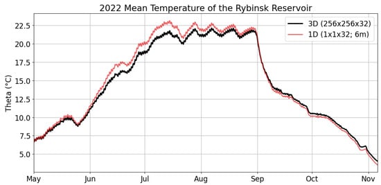
Figure 15.
The mean temperature of the reservoir calculated in the full (three-dimensional) configuration of the model and the simplified (one-dimensional) configuration, with a prescribed depth matching the heat content of the 3D simulation.
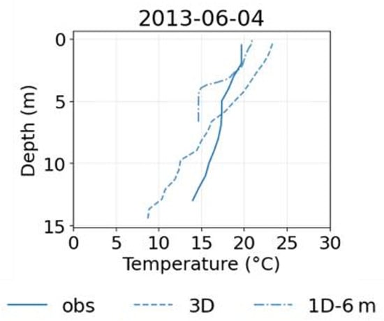
Figure 16.
Vertical temperature distribution for the Koprino station (obtained using field observations and numerical modeling in full and simplified (with depth clarification) model configurations).
To study the formation of seiches and their characteristic frequencies, an additional numerical experiment was carried out: a full three-dimensional configuration of the model with a given bathymetry was used, but all of the atmospheric forcing variables were taken to be equal to zero except for the horizontal component of the momentum flux (corresponding to the predominant (western) wind direction for the Rybinsk Reservoir region), which was periodic with a period of 24 h. As an initial condition in the idealized formulation, a linear vertical temperature distribution with a gradient of 1.5 degrees Celsius per meter was set, which corresponds to the buoyancy frequency N = 4 × s−1. A time interval of one summer month was chosen, where the most pronounced thermocline was observed. The points located in different zones of reservoirs (coastal zone, deep-water zone, and river inflow zone) and at different depths were selected relative to when the location of the thermocline in the calculation period (see Figure 17).
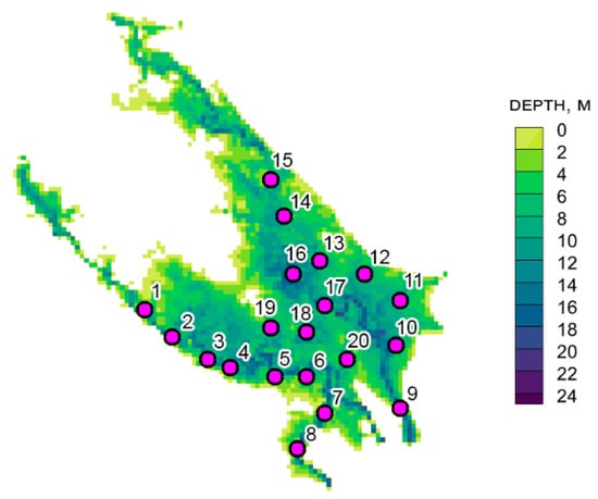
Figure 17.
Map of the locations (as represented on the model grid resolution) of the Rybinsk Reservoir that were selected for the study of the characteristic frequencies of temperature fluctuations.
Fourier spectra were calculated based on the time series of temperature changes at the points under consideration to identify characteristic oscillation frequencies. In the experiment with idealized forcing (see Figure 18), the frequency associated with the diurnal wind cycle (at a frequency of approximately 0.8 × Hz, which corresponds to a period of about a day) and the intradiurnal frequencies reflecting seiche harmonics (from two hours—on the graph these are frequencies from —to a day) are clearly distinguished.
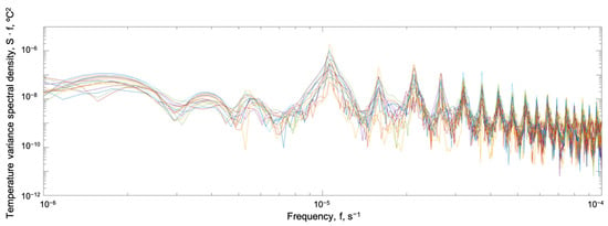
Figure 18.
The Fourier spectrum of the temperature fluctuations, multiplied by frequency, at different points of the Rybinsk Reservoir (obtained in a formulation with periodic meteorological forcing). Different points of the reservoir are marked with different colors.
Simple seiche parameterizations (such as, for example, the parameterization in [24]) for the first horizontal mode in such conditions will not be able to reproduce all of the observed oscillations. Note that such parameterizations can work well in conditions of small reservoirs with simple morphometry (such as, for example, Lake Kuivajärvi in Finland (see [44])), and this is in contrast to the water body identified in this study, which has a complex bathymetry. To account for the effects associated with seiche oscillations in water bodies with complex morphometry, it is necessary to check the applicability and, if necessary, revise the seiche oscillation parameterizations.
Note that, for the model results obtained with realistic atmospheric forcing (which were used in the main series of numerical experiments in this study), temperature fluctuation spectra were also constructed, where a much smoother distribution of spectral density was observed and a connection with the reservoir morphometry was noted (for example, for the zone near the island, see Point 19 in Figure 17). To study seiches in a complex reservoir with physical forcing, continuous temperature measurement data are needed at least in the summer months, which is when a pronounced thermocline is observed, to compare the real and model oscillation frequencies. Thus, we believe that such a detailed analysis will require a separate study and discussion.
The configuration of the numerical model for the Rybinsk Reservoir proposed in this study allows us to reproduce the thermal structure and can be used in further studies of biochemical processes in the reservoir, including for methane emissions. It should also be noted that the water object selected for research—the Rybinsk Reservoir—is not a typical inland artificial water body. Its morphometry can be described as the basin–valley type. This means that, in some aspects of a hydrological or thermodynamical regime, the Rybinsk Reservoir is more similar to natural lakes than to valley-type reservoirs. For this reason, the structure of the internal circulation of studied reservoir was complicated. For example, during the summer period, large-scale water circulation can cover the entire central part of the water body. Circulation patterns in reservoirs strongly depend on the wind primary direction, and the scales of motion can vary a great deal depending on the atmospheric forcing [45]. In such a case, the usage of a 3D model is necessary for correct simulation of internal water dynamics. Some examples of water circulation patterns, according to the model calculations, were presented in Section 4.2.2 of this article. The results of the 3D model application on the Rybinsk Reservoir can be also very useful for further studies of natural lake simulations. A model capable of reproducing the complex water dynamics in a basin–valley reservoir can often be confidently applied to simpler natural lakes in terms of morphometry. Thus, the research tool presented in the current work is planned to be used to study not only artificial reservoirs, but also natural terrestrial water bodies.
Author Contributions
Conceptualization, D.S.G., V.A.L., and E.V.M.; methodology, D.S.G., V.A.L., E.V.M., A.V.Z., and V.I.L.; software, D.S.G. and E.V.M.; validation, V.A.L., D.S.G., and R.A.A.; formal analysis, D.S.G., V.A.L., and E.V.M.; investigation, D.S.G., V.A.L., R.A.A., and E.V.M.; data curation, A.V.Z. and V.I.L.; writing—original draft preparation, D.S.G. and V.A.L.; writing—review and editing, D.S.G. and E.V.M.; visualization, V.A.L. and R.A.A.; supervision, E.V.M.; project administration, D.S.G.; funding acquisition, D.S.G. All authors have read and agreed to the published version of the manuscript.
Funding
This research was funded by the Russian Scientific Foundation under grant number 23-77-01032 (development and configuration of a three-dimensional model, systematization of field measurements data); by the FSTP project “Research in geophysical boundary layers and the development of new modelling approaches for Earth system models” within the program “Improvement of the global world-level Earth system model for research purposes and scenarios forecasting of climate change” (conducting numerical experiments with 1D configuration and processing modeling data); and by the Ministry of Education and Science of the Russian Federation as part of the program of the Moscow Center for Fundamental and Applied Mathematics under agreement № 075-15-2025-345 (statistical assessments of the agreement between model results and measurement data).
Data Availability Statement
The datasets generated during and analyzed during the current study are available from the corresponding authors on reasonable request.
Conflicts of Interest
Author Ramil A. Ahtamyanov was employed by the company Hydrometcenter. The remaining authors declare that the research was conducted in the absence of any commercial or financial relationships that could be construed as a potential conflict of interest.
References
- Downing, J.A.; Prairie, Y.; Cole, J.; Duarte, C.; Tranvik, L.; Striegl, R.G.; McDowell, W.; Kortelainen, P.; Caraco, N.; Melack, J.; et al. The global abundance and size distribution of lakes, ponds, and impoundments. Limnol. Oceanogr. 2006, 51, 2388–2397. [Google Scholar] [CrossRef]
- Messager, M.L.; Lehner, B.; Grill, G.; Nedeva, I.; Schmitt, O. Estimating the volume and age of water stored in global lakes using a geo-statistical approach. Nat. Commun. 2016, 7, 13603. [Google Scholar] [CrossRef]
- Jacobs, J.D.; Grondin, L.D. The influence of an Arctic large-lakes system on mesoclimate in south-central Baffin Island, NWT, Canada. Arct. Alp. Res. 1988, 20, 212–219. [Google Scholar] [CrossRef]
- Krinner, G. Impact of lakes and wetlands on boreal climate. J. Geophys. Res. Atmos. 2003, 108, D16. [Google Scholar] [CrossRef]
- Thiery, W.; Davin, E.L.; Panitz, H.J.; Demuzere, M.; Lhermitte, S.; Van Lipzig, N. The impact of the African Great Lakes on the regional climate. J. Clim. 2015, 28, 4061–4085. [Google Scholar] [CrossRef]
- Elliott, J.; Jones, I.; Thackeray, S. Testing the sensitivity of phytoplankton communities to changes in water temperature and nutrient load, in a temperate lake. Hydrobiologia 2006, 559, 401–411. [Google Scholar] [CrossRef]
- Winder, J.C.; Braga, L.P.; Kuhn, M.A.; Thompson, L.M.; Olefeldt, D.; Tanentzap, A.J. Climate warming has direct and indirect effects on microbes associated with carbon cycling in northern lakes. Glob. Change Biol. 2023, 29, 3039–3053. [Google Scholar] [CrossRef]
- Grechushnikova, M.; Grigoryeva, I.; Lomova, D.; Kremenetskaya, E.; Komissarov, A.; Fedorova, L.; Lomov, V.; Chekmareva, E. Formation of the Hydroecological Structure of the Ivankov Reservoir in the Summer in Adjacent Years under Different Weather Conditions. Izv. Atmos. Ocean. Phys. 2024, 60, 320–333. [Google Scholar] [CrossRef]
- Schulz, S.; Matsuyama, H.; Conrad, R. Temperature dependence of methane production from different precursors in a profundal sediment (Lake Constance). FEMS Microbiol. Ecol. 1997, 22, 207–213. [Google Scholar] [CrossRef]
- Zeikus, J.; Winfrey, M. Temperature limitation of methanogenesis in aquatic sediments. Appl. Environ. Microbiol. 1976, 31, 99–107. [Google Scholar] [CrossRef]
- Geller, W. The temperature stratification and related characteristics of Chilean lakes in midsummer. Aquat. Sci. 1992, 54, 37–57. [Google Scholar] [CrossRef]
- Goudsmit, G.H.; Burchard, H.; Peeters, F.; Wüest, A. Application of k-ε turbulence models to enclosed basins: The role of internal seiches. J. Geophys. Res. Ocean. 2002, 107, 23–31. [Google Scholar] [CrossRef]
- Stepanenko, V. Parameterization of seiches for a one-dimensional model of a reservoir. Tr. Mosk. Fiz. Tekh. Inst. 2018, 10, 97–111. [Google Scholar]
- Goncharov, A.; Bolotov, S.; Puklakov, V.; Malashenkov, D.; Erina, O.; Lomov, V. Vertical water structure and reservoir plankton in spring. Inland Water Biol. 2022, 15, 437–445. [Google Scholar] [CrossRef]
- Chen, Z.; Huang, P.; Zhang, Z. Interaction between carbon dioxide emissions and eutrophication in a drinking water reservoir: A three-dimensional ecological modeling approach. Sci. Total Environ. 2019, 663, 369–379. [Google Scholar] [CrossRef]
- Deltares. Delft3D-FLOW User Manual; Deltares: Deltares, The Netherlands, 2023. [Google Scholar]
- Kranenburg, W.; Tiessen, M.; Veenstra, J.; de Graaff, R.; Uittenbogaard, R.; Bouffard, D.; Sakindi, G.; Umutoni, A.; Van de Walle, J.; Thiery, W.; et al. 3D-modelling of Lake Kivu: Horizontal and vertical flow and temperature structure under spatially variable atmospheric forcing. J. Great Lakes Res. 2020, 46, 947–960. [Google Scholar] [CrossRef]
- Tran, N.; Nguyen, T.; Nguyen, T.; Doan, T.; Nguyen, T.; Dao, T. Simulation of Water Quality in Bung Binh Thien Lake, An Giang Province, Vietnam, Using the Delft3D Model. Int. J. Geoinformatics 2024, 20, 56–71. [Google Scholar]
- MIKE by DHI. MIKE 21 & MIKE 3 Flow Model FM, Hydrodynamic and Transport Module; Scientific Documentation; DHI Water Environments: Southampton, UK, 2017. [Google Scholar]
- Zhang, X.; Duan, B.; He, S.; Lu, Y. Simulation study on the impact of ecological water replenishment on reservoir water environment based on MIKE21—Taking Baiguishan Reservoir as an example. Ecol. Indic. 2022, 138, 108802. [Google Scholar] [CrossRef]
- Xu, M.; Yu, L.; Zhao, Y.; Li, M. The simulation of shallow reservoir eutrophication based on MIKE21: A case study of Douhe Reservoir in North China. Procedia Environ. Sci. 2012, 13, 1975–1988. [Google Scholar] [CrossRef]
- Gladskikh, D.; Mortikov, E. On Parameterization of Dissipative Processes in Turbulent Transport Models for Description of Thermohydrodynamics and Biogeochemistry of Stratified Inland Water Bodies. Izv. Atmos. Ocean. Phys. 2024, 60, 286–296. [Google Scholar] [CrossRef]
- Mortikov, E.V.; Glazunov, A.V.; Lykosov, V.N. Numerical study of plane Couette flow: Turbulence statistics and the structure of pressure–strain correlations. Russ. J. Numer. Anal. Math. Model. 2019, 34, 119–132. [Google Scholar] [CrossRef]
- Gladskikh, D.; Stepanenko, V.; Mortikov, E. The effect of the horizontal dimensions of inland water bodies on the thickness of the upper mixed layer. Water Resour. 2021, 48, 226–234. [Google Scholar] [CrossRef]
- Lomov, V.; Frolova, N.; Efimov, V.; Repina, I.; Zhe, L.; Liu, Y. Variability of methane content and fluxes in the rybinsk reservoir based on field observations in different seasons of the year. Izv. Atmos. Ocean. Phys. 2024, 60, 473–489. [Google Scholar] [CrossRef]
- Lazareva, V.; Mineeva, N.M. Structure and functioning of Rybinsk reservoir ecosystem in the beginning of XXI century. Inland Water Biol. Inst. RAS 2018, 17, 465. [Google Scholar]
- Bogoslovsky, B.; Fil, S. Classification of Water Bodies by External Water Exchange; Geography Community USSR: Leningrad, Russia, 1984; pp. 54–60. [Google Scholar]
- Litvinov, A.; Roshchupko, V. Long-term and seasonal water level fluctuations of the Rybinsk Reservoir and their role in the functioning of its ecosystem. Water Resour. 2007, 34, 27–34. [Google Scholar] [CrossRef]
- Korneva, L.G.; Lazareva, V.I.; Mineeva, N.M.; Sigareva, L.E.; Sokolova, E.A.; Timofeeva, N.A.; Mitropol’skya, I.V.; Solovyeva, V.V. The state and dynamics of biological communities in the Rybinsk Reservoir under climate changes. J. Sib. Fed. Univ. Biol. 2019, 12, 160–179. [Google Scholar] [CrossRef]
- Morinishi, Y.; Lund, T.S.; Vasilyev, O.V.; Moin, P. Fully conservative higher order finite difference schemes for incompressible flow. J. Comput. Phys. 1998, 143, 90–124. [Google Scholar] [CrossRef]
- Pacanowsky, R.C.; Philander, S.G.H. Parameterization of vertical mixing in numerical models of tropical oceans. J. Phys. Oceanogr. 1981, 11, 1443–1451. [Google Scholar] [CrossRef]
- Burchard, H. Applied Turbulence Modeling in Marine Waters. Lect. Notes Earth Sci. 2002, 100. [Google Scholar] [CrossRef]
- Burchard, H.; Deleersnijder, E. Stability of algebraic non-equilibrium second-order closure models. Ocean. Model. 2001, 3, 33–50. [Google Scholar] [CrossRef]
- Baas, P.; de Roode, S.R.; Lenderink, G. The scaling behaviour of a turbulent kinetic energy closure model for stably stratified conditions. Bound.-Layer Meteorol. 2008, 127, 17–36. [Google Scholar] [CrossRef]
- Schumann, U.; Gerz, T. Turbulent mixing in stably stratified shear flows. J. Appl. Meteorol. Climatol. 1995, 34, 33–48. [Google Scholar] [CrossRef]
- Businger, J.; Wyngaard, J.; Izumi, Y.; Bradley, E. Flux-profile relationships in the atmospheric surface layer. J. Atmos. Sci. 1971, 28, 181–189. [Google Scholar] [CrossRef]
- Dyer, A.J. A review of flux-profile relationships. Bound.-Layer Meteorol. 1974, 7, 363–372. [Google Scholar] [CrossRef]
- Charnock, H. Wind stress on a water surface. Q. J. R. Meteorol. Soc. 1955, 81, 639–640. [Google Scholar] [CrossRef]
- Poddubny, S.A. Modern state and ecological significance of water level in Upper Volga reservoirs. Water Chem. Ecol. 2012, 12, 9–15. (In Russian) [Google Scholar]
- Moriasi, D.N.; Arnold, J.G.; Van Liew, M.W.; Bingner, R.L.; Harmel, R.D.; Veith, T.L. Model evaluation guidelines for systematic quantification of accuracy in watershed simulations. Trans. ASABE 2007, 50, 885–900. [Google Scholar] [CrossRef]
- da Silva, M.G.; de Aguiar Netto, A.d.O.; de Jesus Neves, R.J.; do Vasco, A.N.; Almeida, C.; Faccioli, G.G. Sensitivity analysis and calibration of hydrological modeling of the watershed Northeast Brazil. J. Environ. Prot. 2015, 6, 837–850. [Google Scholar] [CrossRef]
- Hersbach, H.; Bell, B.; Berrisford, P.; Hirahara, S.; Horányi, A.; Muñoz-Sabater, J.; Nicolas, J.; Peubey, C.; Radu, R.; Schepers, D.; et al. The ERA5 global reanalysis. Q. J. R. Meteorol. Soc. 2020, 146, 1999–2049. [Google Scholar] [CrossRef]
- Kalnay, E.; Kanamitsu, M.; Kistler, R.; Collins, W.; Deaven, D.; Gandin, L.; Iredell, M.; Saha, S.; White, G.; Woollen, J.; et al. The NCEP/NCAR 40-Year Reanalysis Project. Renew. Energy Four Vol. Set 2018, 146–194, 15. [Google Scholar]
- Stepanenko, V.; Mammarella, I.; Ojala, A.; Miettinen, H.; Lykosov, V.; Vesala, T. LAKE 2.0: A model for temperature, methane, carbon dioxide and oxygen dynamics in lakes. Geosci. Model Dev. 2016, 9, 1977–2006. [Google Scholar] [CrossRef]
- Lavrova, O.Y.; Korneva, L.G.; Shendrick, V.D.; Soloviev, D.M.; Strochkov, A.Y. Detecting biogenic pollution in Rybinsk Reservoir from satellite data and contact measurements. In Proceedings of the Remote Sensing of the Ocean, Sea Ice, Coastal Waters, and Large Water Regions, Amsterdam, The Netherlands, 24–25 September 2014; Volume 9240, pp. 82–92. [Google Scholar]
Disclaimer/Publisher’s Note: The statements, opinions and data contained in all publications are solely those of the individual author(s) and contributor(s) and not of MDPI and/or the editor(s). MDPI and/or the editor(s) disclaim responsibility for any injury to people or property resulting from any ideas, methods, instructions or products referred to in the content. |
© 2025 by the authors. Licensee MDPI, Basel, Switzerland. This article is an open access article distributed under the terms and conditions of the Creative Commons Attribution (CC BY) license (https://creativecommons.org/licenses/by/4.0/).