Article

Optimized Regulation Scheme of Valves in Self-Pressurized Water Pipeline Network and Water Hammer Protection Research

1
College of Water Resources and Civil Engineering, Xinjiang Agricultural University, Urumqi 830052, China
2
Xinjiang Key Laboratory of Water Resources Engineering Safety and Water Disaster Prevention and Control, Urumqi 830052, China
*
Author to whom correspondence should be addressed.
Water 2025, 17(10), 1534; https://doi.org/10.3390/w17101534
Submission received: 18 April 2025 / Revised: 9 May 2025 / Accepted: 16 May 2025 / Published: 20 May 2025

Abstract

:
This study addresses the water hammer protection challenges in the JH gravity-fed bifurcated pipeline network system in Xinjiang, China. A hydraulic transient numerical model is developed using the one-dimensional method of characteristics and implemented in Bentley HAMMER software to systematically analyze the transient response characteristics under different valve closure schemes, with a focus on revealing pressure fluctuation patterns in branch and main pipelines under various shutdown modes. Key findings include the following: Single-valve linear slow closure reduces the maximum water hammer pressure by 54.7%, while the two-stage closure strategy suppresses pressure extremes below safety thresholds with 73.1% higher efficiency than linear closure. For multi-valve conditions, although two-stage closure eliminates negative pressure risks, most of nodes exhibit transient overpressure exceeding 1.5 times the working pressure. By integrating overpressure relief valves into a composite protection system, the maximum transient pressure is strictly controlled within 1.5× rated pressure, and the minimum pressure remains above −2 mH2O, successfully resolving protection challenges in this complex network. These results provide technical guidelines for the safe operation of gravity-fed pipeline systems in high-elevation-difference regions.

1. Introduction

Since 2014, China has accelerated the modernization and water-saving renovation of large- and medium-sized irrigation districts. The rapid development of high-efficiency water-saving irrigation has significantly improved irrigation water use efficiency while enhancing irrigation and drainage infrastructure [1]. By 2019, the total length of water supply pipelines nationwide reached 920,082.14 km, with an annual water supply capacity of 602.12 billion tons [2]. Two distinct water hammer types are identified: a continuous water column hammer (without phase separation) and a cavitation-induced hammer (with flow interruption and cavity collapse). In long-distance gravity-fed systems operating under steady-state conditions, abrupt flow variations during valve maneuvers trigger transient state transitions [3]. A critical challenge stems from water hammer phenomena induced by rapid valve operations, where transient pressures may escalate to 10–100 times normal operating levels, posing catastrophic risks to pipeline integrity [4]. Complex pipe networks present greater hydraulic challenges than simple pipelines due to increased discharge points, additional valves, and more connection interfaces. When flow velocity changes induce water hammer, the resulting economic losses in such systems substantially exceed those in simple pipelines [5]. With the rapid economic development in Xinjiang region, the construction of long-distance, high-head water conveyance pipelines has intensified to accommodate significant topographic variations. Water hammer phenomena induce severe pressure transients within pipeline systems, triggering potential failures including pipeline rupture, joint loosening, and leakage, which may result in equipment damage and shortened system longevity. Prolonged water hammer effects can progressively degrade pumping equipment and valve integrity, substantially increasing maintenance and operational costs, while ultimately compromising public service reliability and community living standards [6]. Research by Lohrasbi A R demonstrated that controlled extension of valve actuation duration (either opening or closing) can significantly mitigate water hammer pressure magnitudes [7]. Investigations by Karadžić U. revealed that simultaneous closure of dual valves exacerbates column separation phenomena [8]. In gravity-driven water conveyance systems, Wang Z P [9] and Huang Y [10] demonstrated that two-stage valve closure achieves superior pressure suppression and operational efficiency compared with linear closure patterns. Meanwhile, Zhang D.J. [11] and Wang S.S. [12] conducted systematic research on water hammer protection mechanisms and mitigation strategies using Bentley HAMMER software, establishing optimized design frameworks for transient control.
While previous studies have provided valuable insights into valve closure optimization and water hammer protection for linear pipelines, research on multi-bifurcation pipeline networks remains limited. The interaction of water hammer pressures across interconnected branches in such systems necessitates a dedicated investigation of transient flow patterns and valve operation laws in long-distance gravity-fed water transmission networks. This study focuses on the JH gravity-fed bifurcated pipeline system in Xinjiang, China. Using Bentley HAMMER software (10.04.00.108 64-bit), we develop a hydraulic transient model to characterize transient flow behavior under diverse valve closure scenarios and evaluate the efficacy of water hammer protection devices in multi-branched configurations.

2. Mathematical Model

2.1. Control Equations

The system of fundamental differential equations for water hammer consists of the equation of motion (1) and the continuity Equation (2).
H x + 1 g V t + V g V x + f D V | V | 2 g = 0
H t + V H x + sin θ + a 2 g V x = 0
where H is the head of the pressure measuring pipe; x is the distance of the pipe along the pipe axis; V is the flow velocity; t is the time; f is the friction coefficient; D is the diameter of the pipeline pipe; g is the acceleration of gravity; θ is the angle between the pipe axis and the horizontal plane; a is the velocity of the water hammer wave.

2.2. Characteristic Line Method

In this study, numerical simulation is carried out using Bentley HAMMER software, i.e., the eigenline method is used to solve the system of differential equations for water hammer.
C + : H p = C p B p Q p
C : H p = C M B M Q p
where Hp is the head of the gauge tube at point P, m; Cp, Bp are the parameters of the C+ characteristic line; CM, BM are the parameters of the C characteristic line; Qp is the flow rate at point P, m3/s. The formulas for Cp, CM, Bp, BM are shown in Equation (5), Equation (6), Equation (7), and Equation (8), respectively.
C p = H K + B M Q E
C : H p = C M B M Q p
B p = B + R | Q E |
B p = B + R | Q F |
where HK is the head of the gauge pipe at point K, m; HP is the head of the gauge pipe at point P, m; B is the coefficient, calculated as B = a g A ; A is the area of the pipe, m2; QE is the flow rate at point E, m3/s; QF is the flow rate at point F, m3/s; R is the coefficient, calculated as R = f Δ x 2 g D A 2 , and Δx is the spatial step, m.

2.3. Boundary Conditions

The overpressure relief valve, as an active protection device against water hammer, effectively mitigates transient high-pressure impacts in specific pipe sections through a dynamic control mechanism. This mechanism reduces structural damage risks from water hammer waves via the following mechanisms. Threshold-triggered activation: When pipeline pressure exceeds a preset critical value, the valve disc rapidly opens under fluid pressure, enabling directional discharge of excess fluid to achieve system decompression. Self-recovery closure: When pressure returns to the safe reseating range, the valve automatically locks via elastic components, completing the pressure regulation cycle (Figure 1). Compared to conventional fixed-pressure relief devices, this system offers adjustable pressure thresholds, rapid response, and delayed closure capability. These features enable adaptive protection for complex pipeline networks under non-stationary water hammer conditions.
The overpressure relief valve balance equation is expressed as follows:
Q P 1 Q P 2 Q P 3 = 0
H P 1 = H P 2 = H P 3 = H P
where Q P 1 , Q P 2 , Q P 3 are the flow rates upstream, downstream, and in front of the overpressure relief valve, m 3 / s , H P 1 , H P 2 , H P 3 are the pressure heads upstream, downstream and in front of the overpressure relief valve, m, respectively.
When H P does not reach the working pressure head of the overpressure relief valve H max , then Q P 3 = 0 ; when H P exceeds the working pressure head of the overpressure relief valve H max , then the valve opens to relieve the flow. The over-valve flow is
Q P 3 = C d A G 2 g ( H P H 0 )
where Cd for the flow coefficient, AG for the overpressure relief valve after the opening of the overflow cross-section, m2; H0 for the overpressure relief valve after the external pressure head (generally connected to the outside of the atmospheric environment), m.

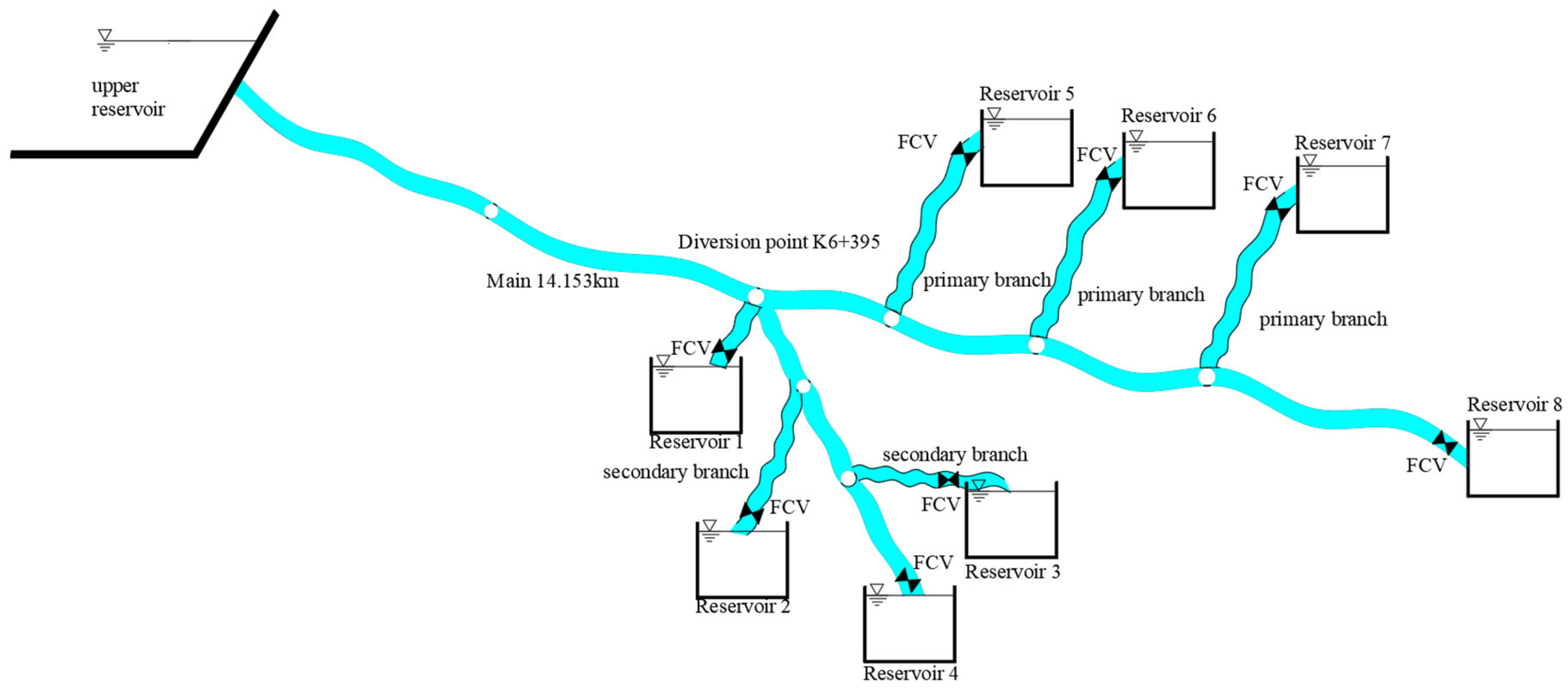
3. Engineering Overview

The JH Project, located in a designated area of Xinjiang, aims to enhance regional agricultural irrigation efficiency and promote sustainable water resource utilization through systematic infrastructure modernization. As a medium-scale irrigation district development initiative, its primary objectives involve upgrading hydraulic infrastructure to increase agricultural water supply reliability, optimizing irrigation water distribution networks for improved farmland productivity, implementing precision water delivery systems to boost crop yields and farmer incomes. Figure 2 illustrates the schematic layout of the high-head gravity-fed bifurcated water conveyance network, comprising elevating farmland irrigation efficiency, thereby increasing crop yields and farmers’ income levels. As shown in Figure 2, the JH high-head gravity-fed water transmission system comprises an upstream reservoir (elevation: 396.4 m), steel pipelines (main pipe: 14.153 km, branches: 4.105 km total), butterfly valves for flow control, and a terminal storage reservoir. The pipes extend to the end of the reservoir through the four sections of gradual change of pipe diameter, namely DN800, DN600, DN400, and DN315.
The first primary branch pipe is laid at the K6+395 stake, with the first secondary branch pipe installed at the 0 m point of the first primary branch pipe. The section 50 m from the water inlet of the first secondary branch pipe is referred to as K1-0+050-1. Similarly, at 2070 m of the first primary branch pipe, the second secondary branch pipe is installed, and the section 50 m from the water inlet of the second secondary branch pipe is referred to as K1-0+050-2. At 3112 m of the first primary branch pipe, the third secondary branch pipe is installed, and the section 50 m from the water inlet of the third secondary branch pipe is referred to as K1-0+050-3. The second primary branch pipe is installed at K10+767, the third primary branch pipe at K11+433, and the fourth primary branch pipe at K12+713. The engineering layout diagram is shown in Figure 2. When configuring parameters in Bentley HAMMER software, the design flow rate of the main pipeline is set to 2700 m3/h, the inlet elevation of the pipeline is 396.4 m, and the pipeline material is steel with a wall thickness of 12 mm. In cases where one or more valves are closed, the valve characteristic curves are set as shown in Figure 3 (using 120 s as an example). Figure 3 illustrates the linear valve closure curve over 120 s and the 20-85-120-100 valve closure curve, both set within Bentley HAMMER software. The 120 s linear curve represents a uniform closure of the valve within 120 s, while the 20-85-120-100 curve indicates a total closure time of 120 s, with the valve being closed to 85% within the first 20 s and the remaining 15% closed over the subsequent 100 s. Similarly, other linear valve closures and two-stage valve closures presented in this paper follow the same principle.

4. Results and Analysis

Through systematic simulation of various accident scenarios, this study determines the maximum water hammer pressure within the pipeline network under each operational condition and evaluates the necessity of implementing pipeline protection measures. In practical irrigation systems, valve closure becomes required upon task completion in each irrigation district. However, heterogeneous irrigation durations across districts, combined with potential undocumented pipeline anomalies (e.g., unexpected reservoir failures), necessitate two distinct valve operation modes: individual branch valve shutdown and coordinated multi-valve shutdown. This paper rigorously investigates both scenarios through transient hydraulic modeling.

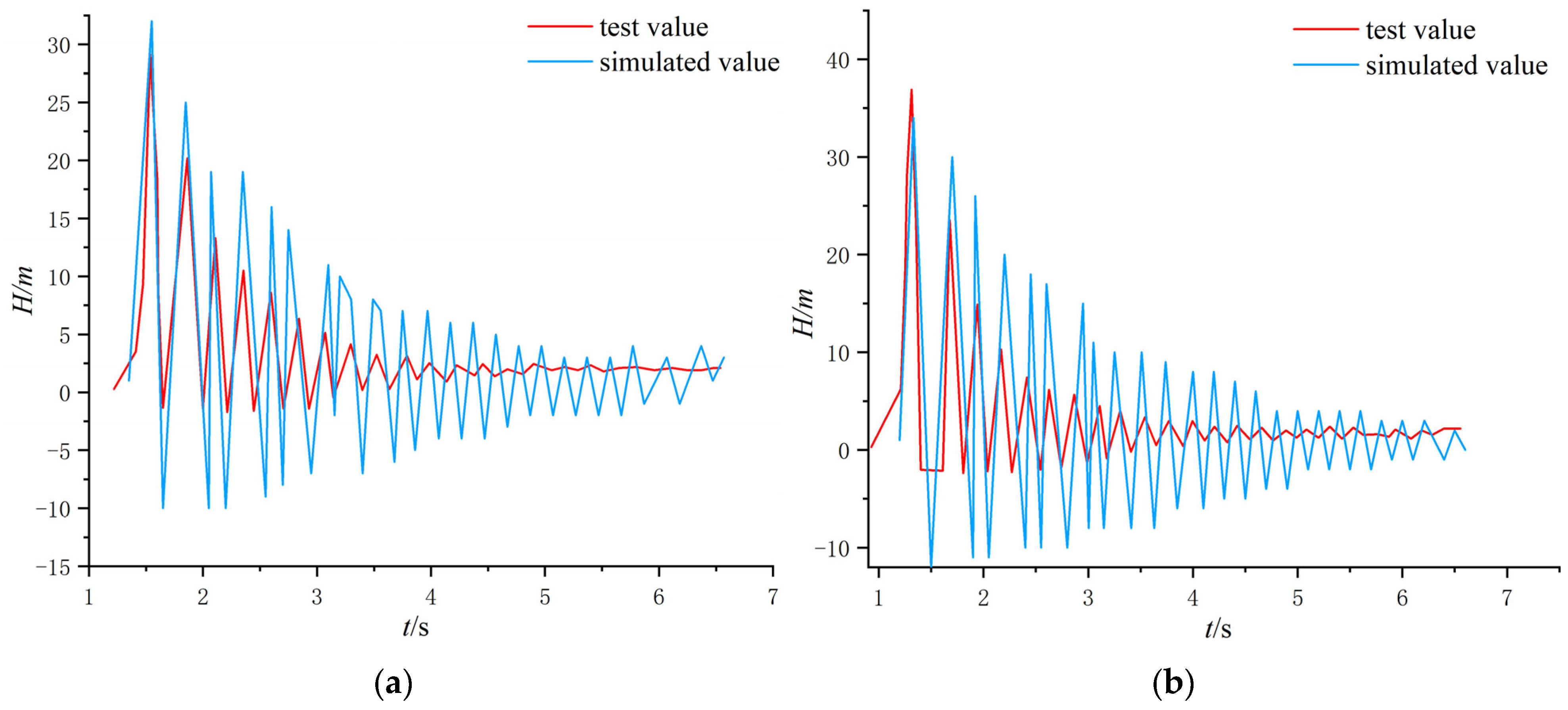
4.1. Model Comparison Validation

This study establishes a one-dimensional mathematical model of water transmission pipelines based on the method of characteristics validated against experimental results for hydraulic transient conditions in branch-type pipe networks reported by Shi Xi et al. [13]. The validation process involves mathematical modeling of their physical test setup under identical operational conditions, specifically obtaining pressure fluctuations upstream of the valve under different closure durations. Comparative analysis between simulation results and experimental data (Figure 4) demonstrates good agreement. For Case 1, the modeled maximum head (Hmax) at the valve reaches 32 m versus experimental 28.9 m, yielding a relative error of 9.6%. For Case 2, the calculated Hmax of 34 m compares with measured 36.5 m, showing 7.4% relative error. Both cases exhibit consistent temporal alignment in achieving peak water hammer pressures. This validation confirms the model’s capability to simulate valve-induced water hammer phenomena with appropriate parameter configuration.

4.2. Water Hammer Characterization of Individual Shut-Off Valve Without Protection

Due to differences in water consumption and usage patterns, the valve closure conditions at the ends of the water distribution network vary. In real-life situations, non-standard valve closures may occur. Through multi-source data research and product parameter comparison, it has been determined that butterfly valves suitable for the four target pipe diameters (DN315/DN400/DN600/DN800) in the current water transmission network system are identified. Based on this, this study sets 10 s as the initial parameter for the linear closure time.
According to the “Design Code for Water Hammer Protection in Pressurized Water Conveyance Pipelines”, the pressure standard for the pipeline before the valve is taken as 1.3 to 1.5 times the static water pressure. In this study, 1.5 times the static water pressure is selected as the pipeline’s pressure value, with the pressure value (negative pressure) set to −2 m. “Closing Pool 1” refers to the individual closure of the butterfly valve before Water Storage Tank 1, and “Closing Pool 2” refers to the individual closure of the butterfly valve before Water Storage Tank 2, with the same principle applied to the others.
To facilitate the comparison of simulation results, each valve is set to close linearly over 10 s. The simulation checks whether the maximum pressure inside the pipeline does not exceed 1.5 times the steady-state operating pressure and whether the minimum pressure is greater than −2 m of water column. The simulation is calculated until the water hammer wave propagation ends, forming a new steady flow state, at which point the simulation concludes. The simulation conditions are shown in Table 1.
Figure 5 shows the comparison of the maximum pressure in the main pipeline when each valve is closed linearly over 10 s. From Figure 5, it can be seen that when the valves before Water Storage Tanks 1 to 7 are closed individually due to the propagation of the water hammer wave. The water hammer wave generated in the secondary branch pipeline spreads into the main pipeline, also affecting the pressure in the main pipeline. The pressure increase in the main pipeline caused by the secondary branches ranges from 1.0 to 1.4 times. When Valve 8 is closed individually, due to the larger pipe diameter, pipe length, and flow rate in the main pipeline, the pressure in the main pipeline exceeds the pressure rating, with the maximum increase occurring at K0+178, where it increases by 7.23 times.
Table 2 presents the maximum pressure before the valve in the pipeline under different valve closing patterns. According to the results of the 10 s linear valve closure in Table 2, it is found that for a 10 s valve closure, except when Valve 1 is closed individually, the transient positive pressure increase in the main pipeline is 1.24-fold. In all other cases of individual valve closure, the pressure increase exceeds 1.5-fold, and the positive pressure inside the pipeline does not meet the requirements. When Valves 6, 7, and the valves before the main pipeline are closed, the negative pressure in the pipeline does not meet the requirements either. To solve this problem, an approach involving extending the linear valve closure time and adopting a two-stage valve closure method is proposed to attempt to reduce the internal pipeline pressure. This section includes 79 calculation scenarios, with the simulation results compared, and eight sets of conditions selected where both positive and negative pressures are closest to the pressure rating, as shown in Table 2.
According to Table 2, extending the linear closure time of Valve 1 to 30 s reduces the maximum instantaneous pressure in the branch pipeline before Water Storage Tank 1 by 8%. For Valves 2 to 8, extending the linear valve closure time reduces the maximum instantaneous pressure by 29.4%, 44.4%, 45.6%, 25.6%, 44.5%, 26.9%, and 54.7%, respectively. For Valves 6 to 8, the negative pressure is eliminated by 87%, 77%, and 100%. Extending the linear valve closure time can ensure that the positive pressure in the pipeline meets the required standards and also helps eliminate the negative pressure. However, extending the valve closure time reduces the efficiency of valve closure. For example, Valve 8, which is located at the end of the main pipeline, has a larger pipe diameter, pipe length, and transient pressure surge due to water hammer. To reduce the transient pressure surge, a longer extension time is needed, which results in low operational economy. Therefore, a two-stage valve closure method is proposed to reduce the water hammer pressure.
As shown in Table 2, compared to the linear slow closure method, the two-stage valve closure method not only reduces the pressure in the pipeline by 10.4%, 33.6%, 46.6%, 45.6%, 27.9%, 48.6%, 29.1%, and 56.2% for Valves 1 to 8, but also eliminates the negative pressure in the pipeline while reducing the maximum pressure within the pipeline to a value below the pipeline’s pressure rating. The two-stage valve closure significantly shortens the valve closure time, improving valve closure efficiency by 33.3%, 66.7%, 73.3%, 75%, 25%, 71.4%, 60%, and 73% for Valves 1 to 8, respectively. Additionally, it helps avoid water resource wastage and holds potential for engineering application. Therefore, in practical engineering, when irrigation tasks are completed in a specific area and require the closure of a valve before a single branch pipeline, the two-stage valve closure method is more effective than linear valve closure in reducing transient positive high pressure and eliminating negative pressure. In cases where a single water storage tank or branch pipeline fails and requires individual valve closure, the two-stage valve closure method, as shown in Table 2, can be referenced.

4.3. Characterization of Water Hammer Under Unprotected Conditions with Multiple Valves Closed at the Same Time

All valves are closed simultaneously using a combined valve closure method, with the closure pattern being a 10 s linear closure. The maximum pressure is checked to ensure that it does not exceed 1.5 times the steady-state operating pressure within the pipeline, and the minimum pressure is verified to be greater than a −2 m water column. The simulation is conducted until the water hammer wave propagation ends and a new steady flow state is established, at which point the simulation ends. The simulation conditions are shown in Table 3 below.
Table 4 shows the maximum and minimum pressures in the branches and main pipe when only the valves between the branches are closed in combination, while Table 5 shows the maximum and minimum pressures in the branches and main pipe when all valves are closed in combination. As seen from Table 4, when multiple valves are closed in a 10 s linear fashion under different operating conditions, the maximum positive pressure in the pipeline does not meet the required standard, and the minimum negative pressure in some parts does not meet the requirement. Moreover, when the valves between the branches are closed in combination, and the main pipe valves remain open while the other valves are closed, the maximum pressure in the main pipe occurs near K12+953, i.e., close to the water split point of the terminal branch.
Comparing Table 4 and Table 5, it can be observed that when the same number of valves are closed, the maximum pressure in the pipeline when all valves are closed in combination is higher than when only the valves between the branches are closed. With the closure of two to seven valves, the maximum pressure increase is, respectively, 63%, 81%, 82%, 76%, 47%, and 48% greater in the case of all valves closed than in the case of branch-valve closure. Additionally, the maximum pressure in the case of all valves closed occurs before the main pipe valve. Since Valve 8 is located at the end of the main pipe, which has a larger diameter and longer length, the resulting water hammer pressure is larger. Generally, the water hammer pressure in the main pipe is greater than that in the branches. In all operating conditions, the water hammer pressure in the pipeline exceeds the static water pressure by 1.5-fold, indicating that the valve closing method needs optimization.
As shown in Table 5, when multiple valves are closed simultaneously in a 10 s linear fashion under each operating condition, both the maximum and minimum pressures within the pipeline exceed the limits significantly. When valves on Branches 2, 3, 4, 5, 6, 7, and the main pipe’s terminal are closed simultaneously, with the remaining pipelines operating normally, the maximum pressure in Branch 3 and Branch 4 is the highest among all valve combination closing conditions for these branches. This operating condition is referred to as the Most Unfavorable Condition 1 (abbreviated as “Unfavorable 1”). When all valves in front of the reservoirs are closed simultaneously, the maximum pressure in Branches 1, 2, 5, 6, 7, and the main pipe is the highest among all operating conditions for these branches and the main pipe. This condition is referred to as the Most Unfavorable Condition 2 (abbreviated as “Unfavorable 2”). In conclusion, when multiple valves are closed simultaneously, the maximum pressure in each branch and the main pipe exceeds the pressure rating, and cavitation occurs in most sections of the pipeline. Therefore, pressure reduction measures must be implemented when multiple valves are closed simultaneously. If the overpressure issues in the pipeline for conditions Unfavorable 1 and Unfavorable 2 are addressed, the problems in other operating conditions will also be resolved. A two-stage valve closure method is used for numerical simulation for conditions Unfavorable 1 and Unfavorable 2, adjusting the duration of the first stage of closure and the setpoint opening. A total of 46 two-stage valve closure schemes are adopted, with six sets of schemes with relatively smaller valve pressures displayed in Table 6. By comparing the pipeline pressures of different schemes, the most suitable valve closing pattern is selected.
Table 6 presents the maximum and minimum pressures in branch pipes and main pipelines under the two most unfavorable operating conditions during simultaneous valve closure. As shown in Table 5, although the two-stage valve closure strategy effectively eliminates negative pressures within the pipeline and significantly reduces water hammer pressure, the internal positive pressures under both Worst Case 1 and Worst Case 2 conditions still exceed allowable limits. This indicates that sole optimization of valve closure procedures cannot meet pipeline safety operation standards, necessitating the installation of water hammer protection devices for additional pressure reduction. Comparative analysis between Table 6 and Table 7 reveals that the 20-85-120-100 valve closure pattern achieves pressure reductions of 62.3%, 70.1%, 74.5%, 74.6%, 57.1%, 58%, 57.8%, and 58.9%, respectively, in Branch Pipes 1–7 and the main pipe under Worst Case 1 condition. For Worst Case 2 condition, the corresponding pressure reductions reach 69.6%, 74.5%, 72%, 73%, 61.2%, 65.2%, 64.2%, and 62.2%. This closure pattern not only demonstrates substantial pressure mitigation but also completely eliminates negative pressures under both operating conditions. Based on these results, we propose implementing overpressure relief valves in conjunction with the 20-85-120-100 closure strategy to further reduce pipeline pressures.

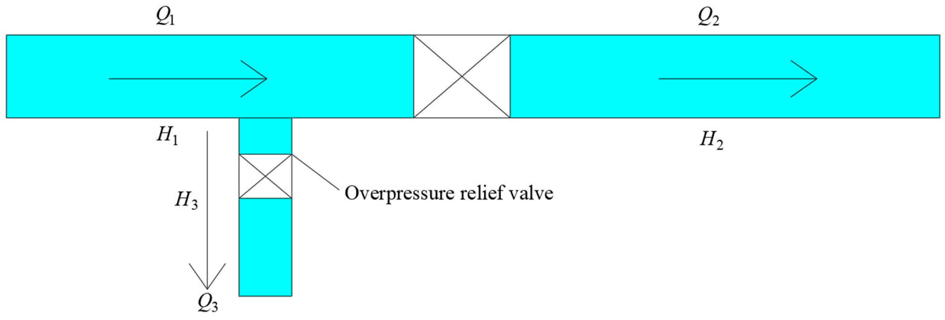
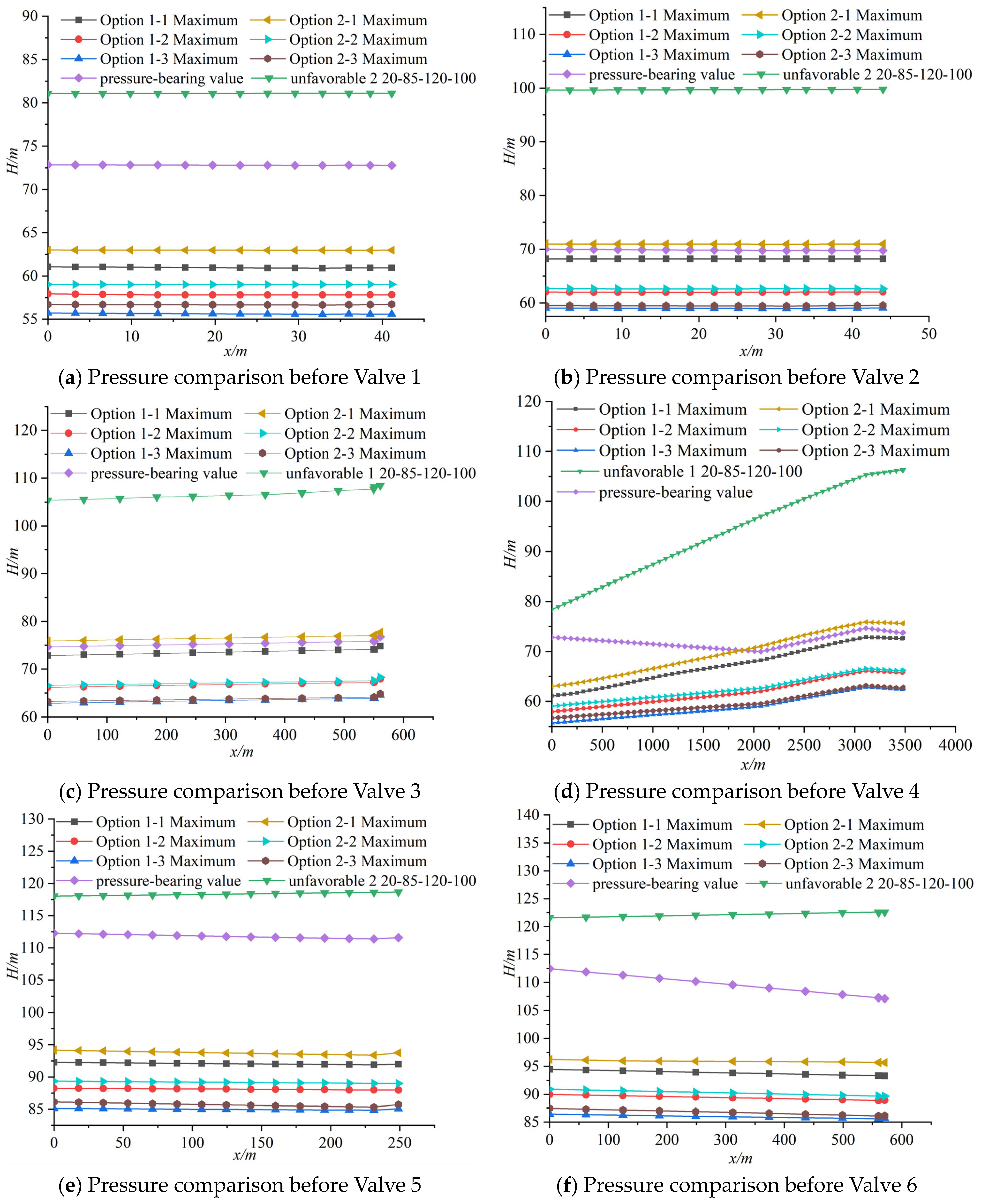
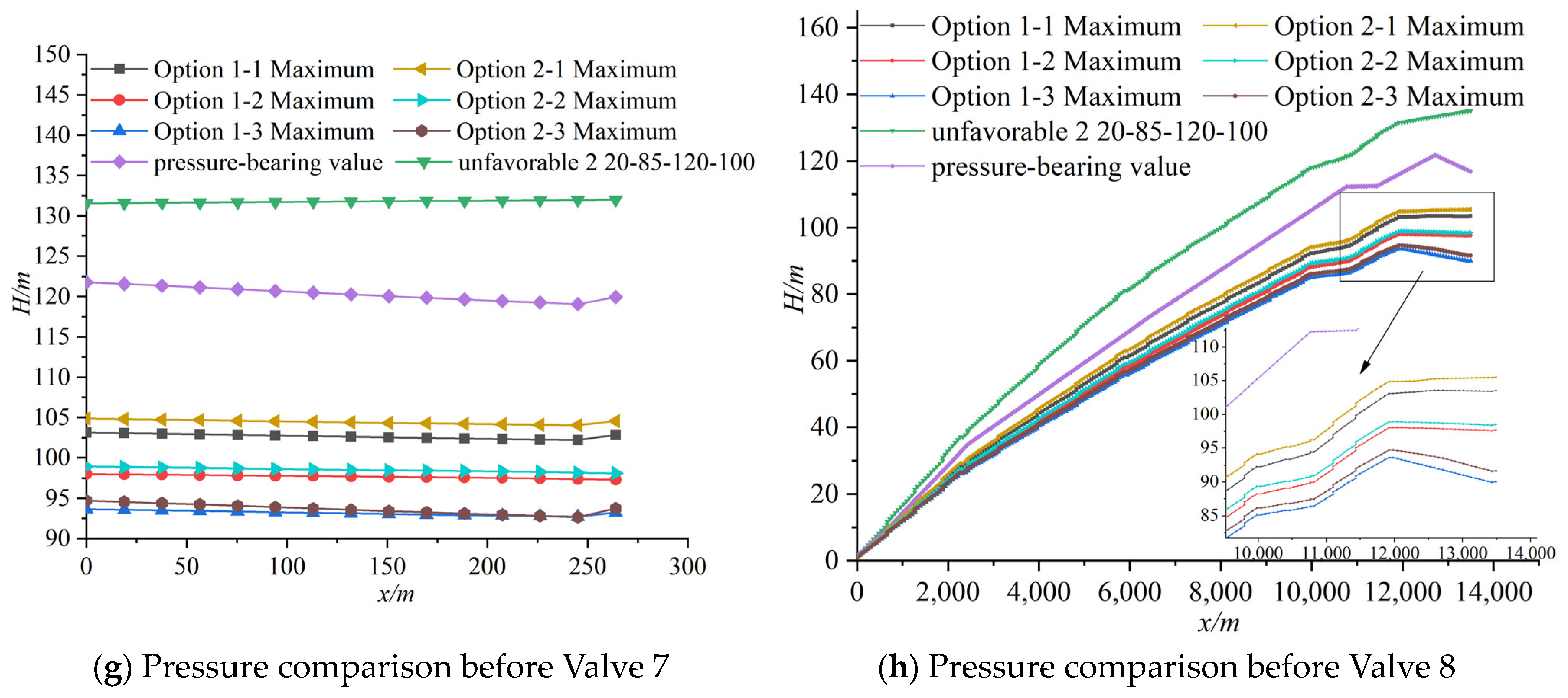
4.4. Analysis of Pipeline Water Hammer When an Overpressure Relief Valve Is Installed in Front of the Valve

According to the “Technical Regulations for Long-Distance Water Transmission Pipelines (Channels) in Urban Water Supply”, the requirements for selecting pressure relief valves are as follows:
(1)
The nominal diameter of the pressure relief valve should be between 1/5 and 1/4 of the diameter of the main pipeline. If the pressure inside the pipeline is high and the flow rate is large, the specifications of the pressure relief valve should be recalculated.
(2)
The set pressure of the pressure relief valve is typically the relief pressure value of the valve. It is advisable to use 1.2 to 1.3 times the maximum steady-state pressure, and it should not be less than the maximum working pressure plus 0.15 MPa to 0.2 MPa.
(3)
As the secondary protection measure for water hammer protection in the water transmission system, the pressure relief valve should respond quickly to high-speed water hammer waves. It should be installed at the node where the water hammer pressure rise is maximum, or the transient pressure or overpressure is the highest, with the installation position as close as possible.
This project is a gravity flow water transmission pipeline network. Under the Most Unfavorable Conditions 1 and 2, the maximum pressure in each branch and the main pipe occurs before the valve. Therefore, in this simulation, the installation location of the pressure relief valves is set to be 5 m before the valves at the ends of each branch and the main pipeline, with a total of eight pressure relief valves installed.
We let λ be the ratio of the pressure relief valve diameter to the pipeline diameter, and β be the difference between the set pressure and the maximum working pressure of the pipeline. Based on engineering experience from similar cases [14], β is set to 0.2 for preliminary calculations. For λ , pressure relief valves with diameters of 0.2, 0.225, and 0.25 are selected for analysis. The parameters of the pressure relief valves and the classification of the schemes are shown in Table 8, and the simulation results under the composite protection system are shown in Figure 6.
From Figure 6, it can be seen that for the positive pressure protection effect, the order of effectiveness is Scheme 2-1 > Scheme 1-1 > Scheme 2-2 > Scheme 1-2 > Scheme 2-3 > Scheme 1-3. From Figure 6a, it can be observed that in this set of data, the maximum pressure in the pipelines of all six schemes is less than the pressure rating. Scheme 2-1 has a maximum pressure greater than the other five schemes. The pipeline pressures in the six schemes are 13.1–23.5% lower than the pressure rating, and the pressures are 27.2–31.3% lower compared to the Most Adverse Operating Condition 2 using the 20-85-120-100 valve closing. Similarly, from Figure 6b,c, Scheme 2-1 has a maximum pressure that is at most 2.8% and 2.7% higher than the pressure rating, respectively. Only Scheme 2-1 fails to meet the required pressure, but the pipeline positive and negative pressures in the other five schemes all meet the requirements. From Figure 6b, the pipeline pressures in the six schemes are 28.8–40.1% lower compared to the Most Adverse Operating Condition 2 using the 20-85-120-100 valve closing. From Figure 6c, the pipeline pressures in the six schemes are 27.9–20.3% lower compared to the Most Adverse Operating Condition 1 using the 20-85-120-100 valve closing (Most Adverse 1 has the highest pressure in Branch Pipes 3 and 4). From Figure 6d, it can be seen that the maximum pressure of Scheme 2-1 exceeds the pressure rating before 2000 m. This is because K1-0+000-2 and K1-0+000-3 are the starting points of the second and third secondary branch pipes, which leads to a decreasing trend in the working pressures at these two locations, and consequently a corresponding decrease in the pressure rating. Therefore, except for Scheme 2-1, the pipeline positive and negative pressures in the other five schemes all meet the requirements. From Figure 6e–h, it can be seen that the pipeline positive and negative pressures in all six schemes meet the requirements. The Most Adverse Condition 2 has relatively high pressures in the corresponding branch pipes in each figure, and Scheme 2-1 has a smaller pressure relief valve outlet diameter compared to Schemes 2-2 and 2-3. Therefore, in the six schemes, Scheme 2-1 has a higher pressure than the other five schemes. In Figure 6e–g, the pipeline pressures in the six schemes are 16.2–24.2%, 9.8–23.14%, and 13.3–20.6% lower compared to the pressure rating, respectively. The pipeline pressures in the six schemes are 20.2–27.9%, 20.8–28.9%, and 20.3–26.6% lower compared to the Most Adverse Operating Condition 2 using the 20-85-120-100 valve closing. In Figure 6h, the maximum pressure before the valve in all six schemes is 9.7–22.9% lower than the pressure rating, and the maximum pressure before the valve in all six schemes is 21.8–33.3% lower compared to the Most Adverse Operating Condition 2 using the 20-85-120-100 valve closing.
Through trial calculation, it is feasible to set β as 0.2. After conducting multi-source data research and comparing product parameters, it is found that when λ is 0.225 and 0.25, the prices of the overpressure relief valves with the two discharge openings differ only slightly. However, the protection effect is better when the diameter is 0.25. Therefore, a pressure relief valve with a nozzle diameter of 0.25 for λ and 0.2 for β is chosen as the most suitable water hammer protection device to meet the engineering requirements.

5. Conclusions

This paper systematically analyzes the transient response characteristics of the pipeline network system under different valve closing schemes and the water hammer characteristics under various valve closing patterns, using the Bentley HAMMER software platform based on the one-dimensional method of characteristics. A combined protection scheme is also proposed to ensure pipeline safety. The specific conclusions are as follows:
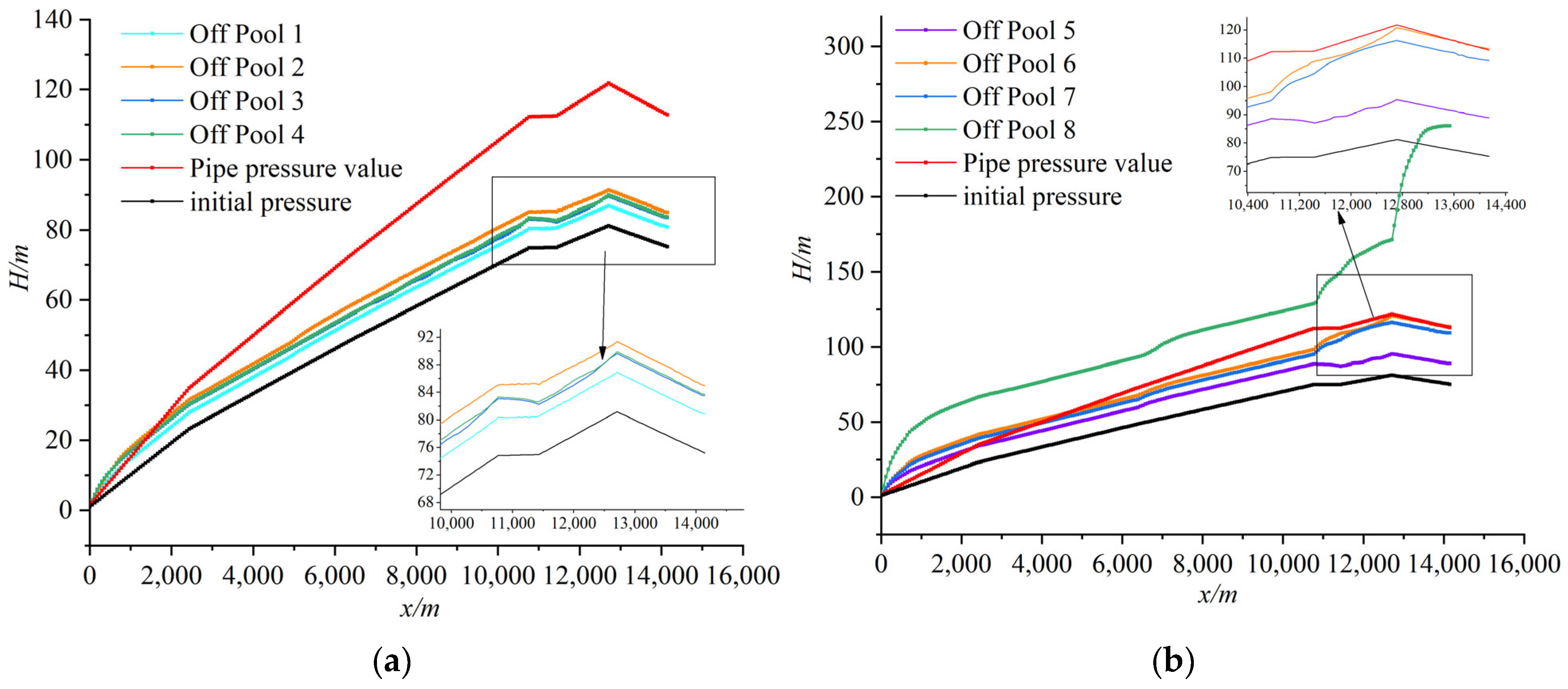
  • Under unprotected conditions, when the valves are closed individually for Valves 1–8, the internal pressure reduction is approximately 10.4%, 33.6%, 46.6%, 45.6%, 27.9%, 48.6%, 29.1%, and 56.2%, respectively, to meet the pressure requirements. The two-stage valve closing improves the valve closing efficiency by 33.3%, 66.7%, 73.3%, 75%, 25%, 71.4%, 60%, and 73%, respectively, compared to linear valve closing.
  • The simultaneous closure of all valves is not the only most unfavorable operating condition. When multiple valves close simultaneously, the maximum pressures in the Most Unfavorable 1 and Most Unfavorable 2 pipelines are the highest among all operating conditions. The maximum pressures in Branches 1–7 and the main pipeline exceed the pressure rating by 268.6%, 479.3%, 457.3%, 467%, 463.3%, 178%, 220%, 211.3%, and 221.3%, respectively.
  • The two-stage valve closing pattern of 20-85-120-100, combined with the overpressure relief valve combination with λ = 0.25 and β = 0.2, forms a joint protection scheme, which reduces the internal pressures in Branches 1–7 by 22%, 14.6%, 15.9%, 15.2%, 23.2%, 19.6%, and 21.9%, respectively, below the pressure rating. It also reduces the maximum pressure in front of the main valve by 21.6%, providing the best protection effect under both individual valve closing and multiple valve simultaneous closing conditions.

Author Contributions

Conceptualization, Y.T., L.L., Q.Z. and Y.Z.; Writing—original draft, Y.Z.; Writing—review & editing, Y.T., L.L. and Q.Z. All authors have read and agreed to the published version of the manuscript.

Funding

Xinjiang Uygur Autonomous Region Major Science and Technology Special Project (2022A02003-4).

Data Availability Statement

The original contributions presented in this study are included in the article. Further inquiries can be directed to the corresponding author.

Conflicts of Interest

The authors declare no conflict of interest.

References

  1. Han, Z. Innovation-driven High-quality Development of Water-saving Irrigation to Strengthen the Foundation of Agricultural Power. China Water Resour. 2023, 7, 11–14. [Google Scholar]
  2. Zhang, M. Research on Valve Closure-Induced Water Hammer and Terminal Reservoir Flow Control in Water Supply Networks; Chang’an University: Xi’an, China, 2021. [Google Scholar]
  3. Wang, C. Calculation of Pump-stopping Water Hammer in Xinjiang Jundong Wucaiwan Water Supply Project. China Water Supply Drain. 2014, 30, 55–57+61. [Google Scholar]
  4. Su, D. Hydraulic Fluctuation and Pipeline Vibration Characteristics During Valve Closure in Water Transmission Pipelines; Xi’an University of Technology: Xi’an, China, 2022. [Google Scholar]
  5. Arefi, M.H.; Ghaeini-Hessaroeyeh, M.; Memarzadeh, R. Numerical modeling of water hammer in long water transmission pipeline. Appl. Water Sci. 2021, 11, 140. [Google Scholar] [CrossRef]
  6. Zhao, Y. Numerical Study of Transient Flow in Viscoelastic Pipes Based on Energy Analysis; Harbin Institute of Technology: Harbin, China, 2022. [Google Scholar]
  7. Lohrasbi, A.R.; Attarnejad, R. Water Hammer Analysis by Characteristic Method. Am. J. Eng. Appl. Sci. 2008, 1, 287–289. [Google Scholar] [CrossRef]
  8. Karadžić, U.; Janković, M.; Strunjaš, F.; Bergant, A. Water Hammer and Column Separation Induced by Simultaneous and Delayed Closure of Two Valves. J. Mech. Eng./Stroj. Vestn. 2018, 64, 525–535. [Google Scholar]
  9. Wang, Z.; Jia, D.; Ma, C. Optimization study of valve closure scheme for long-distance gravity flow water transfer project. People’s Yellow River 2021, 43, 142–146. [Google Scholar]
  10. Huang, Y.; Chen, F. Impact of Terminal Valve Closing Mode on Water Hammer Protection in Long Distance Water Transmission Project. People’s Yangtze River 2018, 49, 70–73. [Google Scholar]
  11. Zhang, D.; Song, X.; Jiang, Y.; Yang, N.; Dong, W. Research on the design of water hammer protection measures for long-distance pressure water transmission projects based on Bentley-Hammer software. Water Supply Drain. 2021, 57, 473–478. [Google Scholar]
  12. Wang, S.; Guo, X. Water Hammer Protection of Air Tank Based on Bentley Hammer. Vib. Shock. 2022, 41, 177–182+244. [Google Scholar]
  13. Shi, X.; Lv, D.; Zhu, D. Experimental and numerical simulation of hydraulic transients in branch-type pipe networks. J. Drain. Irrig. Mach. Eng. 2013, 31, 406–412. [Google Scholar]
  14. Li, N.; Zhang, J.; Shi, L.; Chen, X.; Zhang, X. Joint Water Hammer Protection Characteristics of Air Tanks and Pressure Relief Valves. J. Drain. Irrig. Mach. Eng. 2020, 38, 254–260. [Google Scholar]
Figure 1. Working diagram of overpressure relief valve.
Water 17 01534 g001
Figure 2. Bifurcated water pipeline network layout.
Water 17 01534 g002
Figure 3. Shut-off valve law curve.
Water 17 01534 g003
Figure 4. Pressure fluctuation at the valve under various operating conditions. (a) Pressure fluctuation at Valve 1 during Condition 1; (b) Pressure fluctuation at Valve 2 during Condition 2.
Water 17 01534 g004
Figure 5. Diagram of the maximum pressure envelope of the individual closing valve. (a) Pressure comparison before Valves 1–4; (b) Comparison of pressure before Valve 5–8.
Water 17 01534 g005
Figure 6. Comparison of pressure before each valve. Note: In this set of simulations, under Scenarios 1 and 2, the minimum pressure in the pipeline is greater than the pressure-bearing value (negative pressure), so Figure 6 only shows the maximum pressure.
Water 17 01534 g006aWater 17 01534 g006b
Table 1. Individual shut-off valve simulation table.
Serial NumberOperating ConditionsSpecific Operations
1Steady-state operationThe mainline inlet is a design flow of 2700 m3/h, and the branch lines are all design flows.
2One cistern shut-off valveThere is no protection along the course, the valve in front of the cistern is shut off at 10 s linearly, and the rest of the piping operates normally.
Table 2. Pressure in the main pipe with different shut-off patterns.
Shut-Off Valve PositionValve Closing RegimeRatio of Maximum Pressure to Steady State Pressure in the Tube (min. pressure/m)Valve Closing RegimeRatio of Maximum Pressure to Steady State Pressure in the Tube (min. pressure/m)Valve Closing RegimeRatio of Maximum Pressure to Steady State Pressure in the Tube (min. pressure/m)
110 s linear1.24 (−0.89)30 s linear1.13 (−0.23)10-85-20-1001.11 (1.48)
210 s linear2.11 (−0.62)120 s linear1.49 (−0.16)10-85-40-1001.40 (1.53)
310 s linear2.68 (0.83)150 s linear1.49 (1.48)10-85-40-1001.43 (1.53)
410 s linear2.65 (−0.71)160 s linear1.44 (−0.04)10-85-40-1001.44 (1.40)
510 s linear1.68 (−1.14)40 s linear1.25 (−0.27)10-85-30-1001.21 (1.43)
610 s linear2.65 (−2.55)70 s linear1.47 (−0.33)10-85-20-1001.36 (1.39)
710 s linear1.89 (−2.16)50 s linear1.38 (−0.49)10-85-20-1001.34 (1.51)
810 s linear3.29 (−9.98)260 s linear1.49 (1.49)20-85-70-1001.44 (1.51)
Notes: In this set of simulations, the vaporization pressure is −9.98 m. Therefore, in this table, the minimum pressure in the pipeline for certain operating conditions is represented as −9.98 m, indicating vaporization. Valve Position 1 refers to the valve before Water Storage Tank 1.
Table 3. Simulated working conditions of combined valve shut-off.
Serial NumberCalculation Condition NameConcrete Operation
1Simultaneous valve closure of 2 cisternsUnprotected along the course, 2 cisterns were selected to shut off the valves at 10 s linearly. Other cisterns are functioning normally.
2Simultaneous valve closure of 3 cisternsUnprotected along the course, 3 cisterns were selected to shut off the valves at 10 s linearly. Other cisterns are functioning normally.
3Simultaneous valve closure of 4 cisternsUnprotected along the course, 4 cisterns were selected to shut off the valves at 10 s linearly. Other cisterns are functioning normally.
4Simultaneous closure of 5 cisternsUnprotected along the course, 5 cisterns were selected to shut off the valves at 10 s linearly. Other cisterns are functioning normally.
5Simultaneous closure of 6 cisternsUnprotected along the course, 6 cisterns were selected to shut off the valves at 10 s linearly. Other cisterns are functioning normally.
6Simultaneous closure of 7 cisternsUnprotected along the course, seven cisterns were selected to shut off the valves at 10 s linearly. Other cisterns are functioning normally.
7Simultaneous valve closure of 8 cisternsUnprotected along the course, the 8 cisterns shut off the valves at the same time in a 10 s linear fashion.
Table 4. Pressure in branch and main when combining shutoff valves between branches only.
Number of Shut-Off ValvesRatio of Maximum Pressure to Steady State Pressure in the Tube (min. pressure/m)
Branch 1Branch 2Branch 3Branch 4Branch 5Branch 6Branch 7Supervisor
21.78
(44.49)
1.55
(45.13)
1.46
(48.38)
1.76
(44.64)
1.66
(69.93)
2.68
(44.98)
2.13
(60.89)
2.02
(−1.75)
32.01
(39.49)
1.78
(41.97)
1.66
(45.49)
1.99
(39.65)
1.92
(51.89)
2.71
(53.00)
2.26
(59.95)
2.20
(−2.22)
42.20
(35.03)
2.42
(42.08)
2.19
(45.90)
2.28
(35.35)
1.95
(56.64)
2.71
(54.77)
2.26
(65.99)
2.20
(−2.63)
52.44
(27.23)
3.29
(27.72)
3.17
(27.23)
3.46
(26.05)
2.12
(47.29)
1.75
(45.38)
2.42
(56.02)
2.27
(−2.52)
62.89
(7.28)
5.30
(−9.98)
5.51
(−9.98)
5.66
(−9.98)
2.55
(13.39)
2.93
(2.10)
2.62
(7.86)
2.72
(−9.98)
73.07
(−9.98)
5.41
(−9.98)
5.63
(−9.98)
5.76
(−9.98)
2.73
(−3.80)
3.12
(−1.34)
2.78
(3.31)
2.89
(−9.98)
Table 5. Pressure in each branch and main with all valve combinations closed.
Number of Shut-Off ValvesRatio of Maximum Pressure to Steady State Pressure in the Tube (min. pressure/m)
Branch 1Branch 2Branch 3Branch 4Branch 5Branch 6Branch 7Supervisor
22.38
(31.22)
1.99
(35.90)
1.87
(39.93)
2.37
(31.26)
2.15
(56.96)
2.74
(19.78)
2.69
(38.78)
3.30
(−8.02)
33.08
(−9.98)
2.49
(10.02)
2.33
(14.90)
3.06
(3.91)
2.66
(3.22)
3.46
(−9.98)
3.49
(−9.98)
3.99
(−9.98)
43.42
(−9.98)
2.81
(3.31)
2.58
(5.86)
3.39
(−2.77)
3.01
(−9.98)
3.75
(−9.98)
3.59
(−9.98)
4.00
(−9.98)
53.61
(−9.98)
3.87
(−9.98)
3.56
(5.40)
3.68
(−9.98)
3.04
(−9.98)
3.75
(−9.98)
3.59
(−9.98)
4.00
(−9.98)
63.79
(−9.98)
4.87
(−9.98)
4.71
(−6.23)
4.68
(−9.98)
3.05
(−9.98)
3.75
(−9.98)
3.48
(−9.98)
4.00
(−9.98)
74.19
(−9.98)
7.05
(−9.98)
8.36
(−9.98)
8.51
(−9.98)
3.64
(−9.98)
4.00
(−9.98)
3.84
(−9.98)
4.27
(−9.98)
shut out5.53
(−9.98)
8.69
(−9.98)
8.00
(−9.98)
8.45
(−9.98)
4.17
(−9.98)
4.80
(−9.98)
4.67
(−9.98)
4.82
(−9.98)
Table 6. Worst 2 two-stage shut-off valve pre-valve pressure.
Closing RuleRatio of Maximum Pressure to Steady State Pressure in the Tube (min. pressure/m)
Branch 1Branch 2Branch 3Branch 4Branch 5Branch 6Branch 7Supervisor
10-85-100-1001.72
(37.73)
2.25
(42.63)
2.27
(46.48)
2.31
(37.73)
1.66
(59.56)
1.92
(58.86)
1.72
(65.60)
1.87
(1.00)
20-85-120-1001.68
(44.51)
2.22
(46.56)
2.24
(49.83)
2.28
(44.53)
1.62
(68.42)
1.67
(68.12)
1.67
(75.15)
1.82
(1.00)
20-85-80-1001.77
(35.31)
2.32
(39.23)
2.34
(43.11)
2.38
(35.34)
1.71
(55.77)
1.98
(55.07)
1.77
(62.01)
1.92
(1.00)
20-85-100-1001.80
(33.44)
2.38
(37.98)
2.40
(41.64)
2.44
(33.48)
1.73
(54.65)
2.01
(53.36)
1.79
(59.77)
1.96
(1.00)
30-85-80-1002.17
(17.72)
2.83
(22.56)
2.83
(24.22)
2.87
(17.79)
2.02
(34.95)
2.32
(33.90)
2.07
(38.59)
2.26
(1.00)
30-85-120-1001.72
(41.92)
2.25
(46.56)
2.27
(49.83)
2.31
(41.94)
1.66
(64.85)
1.71
(64.19)
1.72
(71.03)
1.87
(1.00)
Table 7. Worst 1 two-stage shut-off valve pre-valve pressure.
Closing RuleRatio of Maximum Pressure to Steady State Pressure in the Tube (min. pressure/m)
Branch 1Branch 2Branch 3Branch 4Branch 5Branch 6Branch 7Supervisor
10-85-100-1001.66
(41.93)
2.19
(46.56)
2.21
(49.83)
2.25
(41.95)
1.61
(64.83)
1.88
(65.20)
1.67
(71.03)
1.83
(1.00)
20-85-120-1001.60
(44.51)
2.11
(46.56)
2.13
(49.83)
2.16
(44.53)
1.56
(68.40)
1.68
(68.12)
1.62
(75.15)
1.76
(1.00)
20-85-80-1001.58
(39.95)
1.94
(46.31)
1.96
(49.83)
1.98
(39.98)
1.46
(61.78)
1.57
(61.16)
1.51
(68.17)
1.64
(1.00)
20-85-100-1001.74
(38.50)
2.30
(45.55)
2.33
(49.80)
2.37
(38.52)
1.68
(60.72)
1.95
(59.56)
1.74
(66.12)
1.90
(1.00)
30-85-80-1001.70
(25.65)
2.25
(29.56)
2.28
(30.99)
2.31
(25.64)
1.66
(42.51)
1.92
(42.63)
1.72
(47.46)
1.87
(1.00)
30-85-120-1002.06
(41.92)
2.70
(46.56)
2.73
(49.83)
2.77
(41.94)
1.94
(64.82)
2.24
(64.19)
2.00
(71.03)
2.20
(1.00)
Table 8. Parameters of the caliber of the overpressure relief valve.
ProgrammaticWorst Case Scenario λ β (MPa)ProgrammaticWorst Case Scenario λ β (MPa)
1-110.200.22-120.200.2
1-210.2250.22-220.2250.2
1-310.250.22-320.250.2
Disclaimer/Publisher’s Note: The statements, opinions and data contained in all publications are solely those of the individual author(s) and contributor(s) and not of MDPI and/or the editor(s). MDPI and/or the editor(s) disclaim responsibility for any injury to people or property resulting from any ideas, methods, instructions or products referred to in the content.

