Groundwater Potential Mapping Using Optimized Decision Tree-Based Ensemble Learning Model with Local and Global Explainability

Abstract

Identifying potential groundwater areas is of great importance for its sustainable management. This study improves groundwater potential mapping in Fars province, Iran, by integrating Random Forest (RF) and Categorical gradient Boosting (CatBoost) models with a Bayesian optimization algorithm. The Boruta–XGBoost algorithm for selecting the most important features and SHapley Additive exPlanation (SHAP) values increased the local and global interpretability of the models. The results showed that the optimized CatBoost model provided a more accurate and reliable groundwater potential map with an Area Under the receiver operating characteristic Curve (AUC) of 0.8778 and a Root Mean Square Error (RMSE) of 0.3779 compared to the RF with an AUC = 0.8396 and RMSE = 0.4072. The CatBoost model also identified 80% of wells with potential 1 in the very high and high potential classes, as well as 60% of wells with potential 0 in the low and very low potential classes. SHAP analysis highlighted land use/land cover and the terrain roughness index as the most impactful features, while porosity and permeability had minimal influence. Also, the contribution of individual features for each mapping unit in the study area was calculated using SHAP analysis and a map of SHAP values was prepared. The proposed approach offers a comprehensive methodology for groundwater potential mapping, encompassing input data identification, key feature selection, machine learning model optimization, and output explanation. This effective procedure can be applied in other areas and regions, providing valuable insights for decision-makers to manage groundwater resources sustainably and ensure water security.

1. Introduction

Groundwater, as one of the most essential resources on Earth, accounts for 99% of the total liquid freshwater on the planet [1]. It supplies half of the world’s population with water and is crucial for human survival, agricultural activities, and industrial growth [2,3,4]. Globally, the average freshwater demand is distributed as follows: 70% for agriculture, 20% for industrial use, and 10% for household consumption [4]. Additionally, a 20–30% increase in water demand is projected by 2050 [5,6,7]. Furthermore, by 2050, it is expected that 60% of the world’s population will face water shortages or a lack of access to freshwater [8].

Groundwater resources in Iran supply 60% of water needs [9,10], with agriculture consuming 90% of this amount [11]. Due to the concentration of most of the population in areas reliant on groundwater for drinking and irrigation, Iran has become one of the largest consumers of groundwater [9,10]. In recent decades, decreasing precipitation and climate change in Iran lead to an increased need for groundwater [12]. As a result, there has been an 84.9% increase in the number of groundwater extraction wells, rising from 546,000 in 2002 to over 1,000,000 in 2015 [13]. Consequently, excessive groundwater extraction has resulted in a loss of 5.8 billion m³ underground aquifers [12].

The demand for water extraction is increasing globally, particularly in Iran. Therefore, managing groundwater resources is important to ensure water security and sustainability [2,13,14]. One of the first steps in the sustainable management of groundwater resources is developing Groundwater Potential Map (GWPM) to identify potential groundwater areas [2,8,14,15]. Groundwater potential mapping is essential for the sustainable management and utilization of groundwater resources [14,16].

Previous studies on the development of a GWPM have utilized two main approaches, including Multi-Criteria Decision-Making (MCDM) and Machine Learning (ML) models [2,14,17]. Numerous MCDM-based studies appear to mostly integrate Geographic Information System (GIS) with the Analytical Hierarchy Process (AHP) to generate a GWPM [14,18,19,20,21]. For instance, Ray developed a GWPM for Bengal, India, by using an AHP and applying the Technique for Order of Preference by Similarity to Ideal Solution (TOPSIS), achieving an Area Under the receiver operating characteristic Curve (AUC) value of 0.85 [22]. Similarly, Rana et al. utilized an AHP and Weighted Linear Combination (WLC) method to develop a GWPM for the Pabna district of Bangladesh [23]. Likewise, Prapanchan et al. applied a fuzzy AHP and WLC to generate a GWPM for the Pambar sub-basin in India [24].

ML-based models have gained significant attention in the development of GWPMs due to advantages such as integrating data from various scales and sources, generating accurate models, and producing high-precision outputs. Various models, including Support Vector Regression (SVR) [25,26], decision tree-based models [27,28,29,30,31], an Adaptive Neuro-Fuzzy Inference System (ANFIS) [25,32], and Artificial Neural Networks (ANNs) [33,34], have been employed in GWPM developments. For instance, AlAyyash et al. [25] utilized an ANFIS and SVR with metaheuristic optimization algorithms in the Azraq basin in central Jordan. The results demonstrated the high accuracy of the optimized models, with AUC values exceeding 0.95. Similarly, Nugroho et al. employed SVR, a Random Forest (RF) and ANNs in Java, Indonesia [5]. The RF outperformed other models by achieving an accuracy of 0.80. Furthermore, Roy et al. applied K-Nearest Neighbor, ANN, Gradient Boosting Machine, RF, and Support Vector Machine (SVM) models to develop a GWPM. Among these models, the RF and ANNs performed best [35]. Moreover, Sadeghi et al. [16] utilized a Conventional Neural Network (CNN), a Vision Transformer (VIT), and a Boruta–XGBoost algorithm for generating a GWPM and feature selection in Charmahal Bakhtiari province, Iran. The results showed that the VIT outperformed the CNN.

Despite various studies on providing a GWPM using ML models, a research gap remains regarding the development of an appropriate model and the selection of the most influential feature combinations affecting groundwater potential [14]. Some ML models include hyperparameters that optimal values influence their performance and generalization capability [16,36,37]. Moreover, the optimal combination of influencing features may vary depending on the study area. Feature selection is a crucial step in ML models, aiming to eliminate irrelevant features and reduce redundancy to enhance model performance and decrease computational complexity. The failure to determine the optimal hyperparameter values and the presence of redundant features can lead to increased computational complexity, reduced model generalization, and, consequently, overfitting in ML models [16,36,37].

Producing interpretable results as well as achieving high performance is crucial for scientists to make accurate decisions, especially in geoscience [38]. While ML models achieve better results than statistical and traditional methods, they are often hard to interpret. Therefore, finding a way to understand the result of these models is necessary. What is needed is a method that reveals how much each feature influences the model’s output. In preparing a GWPM, which is the objective of this study, it is important to understand the hierarchical nature of model prediction. In other words, how the set of features controls the overall water potential as well as how they carry this out at the mapping unit level. For this purpose, local interpretation methods such as SHapley Additive exPlanation (SHAP) [39] and Local Interpretable Model-Agnostic Explanation (LIME) [40] allow explainable modeling of geographical phenomena. The local explanation of complex geographical phenomena, rather than the global explanation, explains the importance of features for the model output, allowing for the precise determination of the contribution of each feature to the final decision. Most studies rely on feature importance to explain model outputs [16,41,42]. For example, Sadeghi et al. only presented the importance of each feature based on SHAP values for the entire model in preparing the GWPM [16]. Similarly, Alesheikh et al. calculated the impact of features on the land subsidence susceptibility of the entire model [42]. However, in some geographical studies, local explainability techniques have been investigated in combination with ML models [43,44,45]. Given that the local and global explainability of ML models in GWPM preparation has not been fully investigated, SHAP analysis was used for this purpose in this study. SHAP helps scientists achieve this by providing a detailed and transparent breakdown of feature contributions [38]. In addition to local and global explanations, in this study, unlike in previous studies [38,43], the results are interpreted through the spatial pattern of SHAP values for mapping units across the entire study area.

Therefore, this study uses an interpretative approach based on ML models to prepare a GWPM. Hence, after preparing spatial layers to produce a training dataset for groundwater potential prediction, the Boruta–XGBoost feature selection algorithm is used to select the most important features. In the next step, RF and Categorical gradient Boosting (CatBoost) models are used to predict groundwater potential. A Bayesian Optimization Algorithm (BOA) is used to optimize the hyperparameters. Finally, SHAP analysis is used to evaluate the global and local interpretability of the trained models. The importance of the features is also compared with the output of the two trained models, RF and CatBoost, as well as the Boruta–XGBoost algorithm.

In this study, Fars province is selected as the study area. Fars province in southern Iran is a key agricultural region where groundwater is the main water source for irrigation, domestic, and industrial use [46]. Due to frequent droughts and over-extraction—especially in agriculture, which consumes over 90% of the province’s water—groundwater levels have significantly declined [47,48]. These conditions make the region highly vulnerable and highlight the need for accurate groundwater potential mapping to support sustainable water resource management. The main contributions of this study are as follows: (1) selecting the most impactful features for a GWPM using the Boruta–XGBoost algorithm; (2) modeling a GWPM using decision tree-based ML models, as well as RF and CatBoost ones, which are ensemble ML models and can improve accuracy and prevent overfitting; (3) optimizing hyperparameters using a BOA; (4) identifying effective environmental features; (5) determining the feature importance of parameters using RF, CatBoost, and SHAP values; and (6) analyzing the association between model outputs and environmental features both locally and globally using SHAP across the whole study area.

2. Study Area and Data Used

2.1. Study Area

Fars province, covering an area of approximately 123,144 km², is situated in southern Iran (Figure 1). It extends between 27°02′ to 31°40′ latitudes and 50°36′ to 55°34′ longitudes. The province features diverse elevations, ranging from 115 m to 3915 m above sea level (SRTM DEM). The region receives an average annual rainfall of 201 mm, classifying its climate as hyper-arid [49]. According to a land use/land cover (LULC) map, obtained from the Copernicus Global Land Service (CGLS), 48% of Fars province, mainly in the southern and northeastern regions, consists of bare areas, while 25%, located in the central and northwestern parts, is covered with shrubs (Figure 2v). Open forests and agriculture account for 10% and 16%, respectively, while the remaining 1% includes urban areas, closed forests, and water bodies. Given these conditions, modeling groundwater potential is essential for sustainable water resource management in the region.

Fars province exhibits a complex and geologically diverse landscape, shaped significantly by its location within the Zagros Mountain range—part of the broader Alpine–Himalayan orogenic belt. The geological structure comprises a wide array of lithologies, including sedimentary and metamorphic rocks, as well as formations associated with the Fars ophiolite complex. This complex includes igneous rocks such as pillow lavas, sheeted dikes, and gabbros, alongside serpentinites, cherts, and various sedimentary layers. Additionally, the region features Miocene to Pliocene sedimentary sequences, Quaternary volcanic outcrops, and active fault systems, all of which contribute to the area’s intricate hydrogeological dynamics [50]. Fars province, a key agricultural center in Iran, faces increasing groundwater depletion due to drought, desertification, reduced rainfall, rising temperatures, and declining surface water. Mapping groundwater potential is crucial for identifying vulnerable areas and managing groundwater extraction sustainably

Over recent decades, Fars province has faced increasing pressure on its groundwater resources. A significant decline in precipitation—estimated at about 10 mm over the past 20 years—combined with rising temperatures (by approximately 1 °C) and increased annual evaporation (by 230 mm) have led to a negative water balance across many plains. As a result, groundwater depletion has become a critical concern [51].

2.2. Inventory Map

There are 1312 piezometric wells in the study area, each with recorded water height data.

Table 1. Statistics of piezometric wells.

Statistics	Value (m)	Statistics	Value (m)
Minimum	0.30	Standard Deviation	28.46
Maximum	175.15	Median	26.50
Mean	34.31

shows the statistic indices of piezometric wells. The median water height (26.50 m) was calculated, and wells were classified accordingly: those at or below the median were labeled as target 0, while those above the median were labeled as target 1. The classification of wells into potentials of 0 and 1 has been widely used in previous studies [16,27]. Figure 1 illustrates the distribution of these wells, where target 0 and target 1 are marked as a well and non-well, respectively.

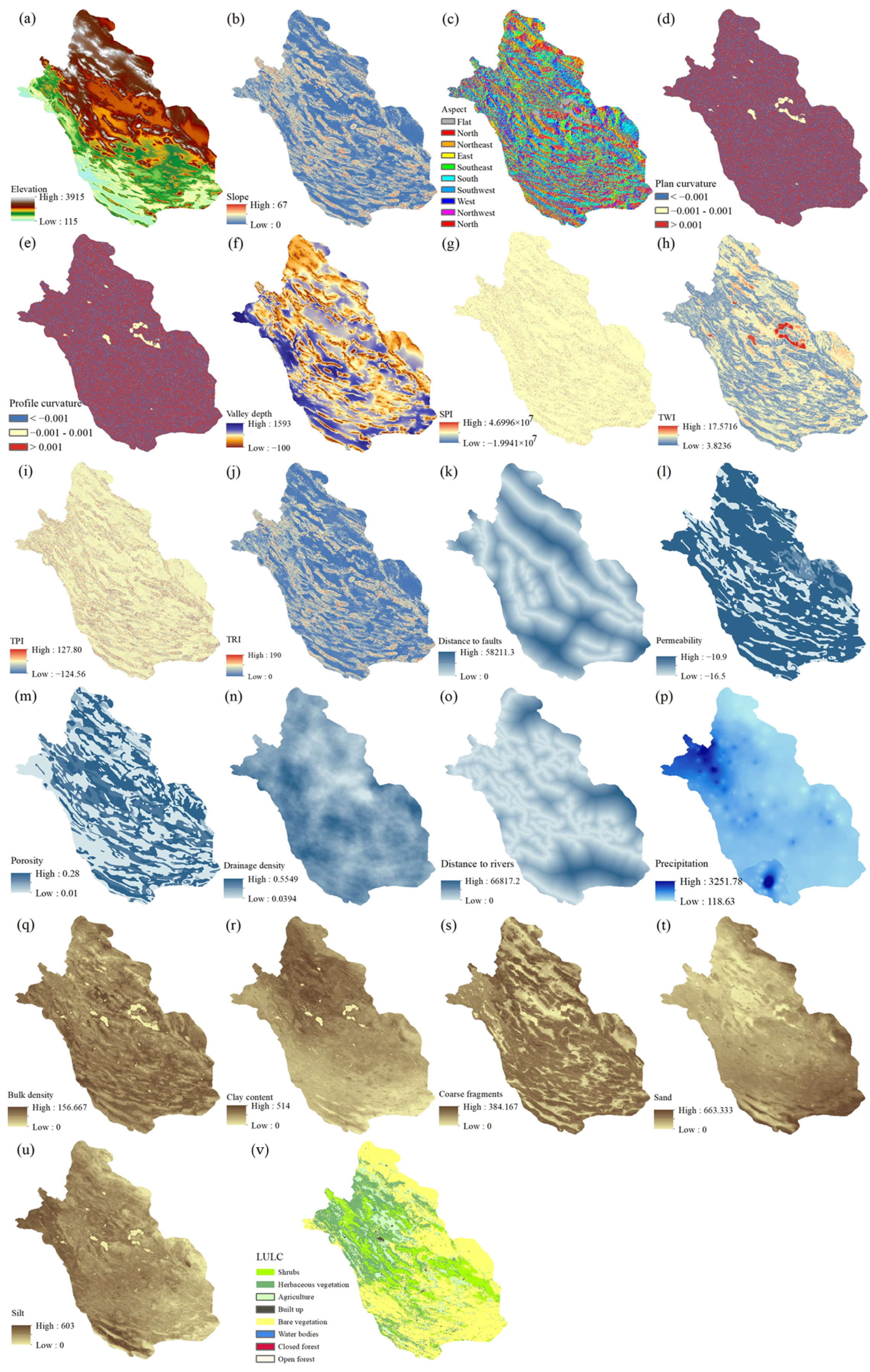
2.3. Environmental Features

Precise groundwater potential mapping requires collecting effective environmental features. After a literature review, 22 environmental features were considered to be fed into the ML models [16,22,33,34,52,53,54] (Figure 2 and

Table 2. Environmental parameters effect on groundwater potential and their sources.

Parameter	Data Source	Resolution/Scale
Elevation (m)	SRTM DEM	30 m
Slope (degree)
Aspect
Plan curvature
Profile curvature
TPI
TWI
TRI
Valley depth (m)
SPI
Sand (g/kg)	International Soil Reference and Information Centre (ISRIC; Soilgrids.org)	250 m
Silt (g/kg)
Clay content (g/kg)
Bulk density (cg/cm3)
Coarse fragment (cm3/dm3)
Permeability (m2)	Global Hydrogeology Maps (GLHYMPSs)	1:100,000
Porosity
Distance to faults (m)	Geological survey and mineral exploration of Iran (GSI)	1:100,000
Distance to rivers (m)
Drainage density
LULC	Copernicus Global Land Service (CGLS)	10 m
Precipitation (mm/year)	Iran Meteorological Organization (irimo.ir)	216 precipitation stations

). These features include the elevation, slope, aspect, plan curvature, profile curvature, topographic position index (TPI), topographic wetness index (TWI), terrain roughness index (TRI), valley depth, stream power index (SPI), sand, silt, clay, porosity, permeability, coarse fragment, distance to faults, distance to rivers, LULC, drainage density, and precipitation. All these features were extracted from six main open sources, namely the Shuttle Radar Topography Mission (SRTM) Digital Elevation Model (DEM), International Soil Reference and Information Centre (ISRIC), geological survey and mineral exploration of Iran (GSI), CGLS, Global Hydrogeology Maps (GLHYMPSs) [55,56], and Iran Meteorological Organization. The environmental features were projected onto the Iran lambert coordinate system with a pixel size of 86 m × 86 m.

The elevation, slope, aspect, profile and plan curvature, TPI, TWI, TRI, SPI, and valley depth were extracted from the SRTM DEM with a resolution of 30 m. These features were projected onto the Iran lambert with a pixel size of 86 m× 86 m. Elevation plays a significant role in groundwater potential, as higher elevations often experience scarce groundwater resources compared to lower elevations, where water accumulates more easily [57]. Additionally, elevation influences vegetation and climate, which affect groundwater recharge distribution [17]. Slopes play a key role in groundwater recharge by controlling rainfall infiltration and runoff [58]. Gentle slopes allow more water to soak into the ground, enhancing recharge, while steep slopes cause rapid runoff, reducing infiltration [17,59]. Due to its impact on water movement, slopes are an important factor in groundwater exploration [58]. The aspect impacts hydrological processes by affecting snowmelt, rainfall direction, and plant growth, all of which influence groundwater recharge patterns [60]. The profile curvature measures the steepest slope direction, while the plan curvature evaluates the slope perpendicular to the profile curvature direction. Both features play a crucial role in shaping water flow patterns, influencing flow convergence and divergence [16]. The TPI measures a location’s elevation relative to its surrounding area in a DEM (Equation (1)). Positive TPI values indicate higher elevations, while negative values represent lower areas [61]. This metric helps analyze a terrain slope and its impact on groundwater recharge, which has an inverse relationship with the TPI.

$$TPI=T_0-{\displaystyle \frac{{{\displaystyle \sum }}_{n-1}{T}_n}{n}} ,$$

(1)

Here, $T_0$ represents the altitude, while $T_n$ refers to the altitude of the grid raster. The variable $n$ denotes the total number of surrounding units within the defined neighborhood. The TWI reflects the influence of topography on groundwater infiltration and helps assess topographic control over hydrological processes [62]. Higher TWI values are typically observed in flat areas prone to frequent flooding, indicating greater groundwater potential, while lower values correspond to regions with lower infiltration capacity [63,64]. The TWI can be calculated as follows:

$$TWI={\displaystyle \frac{Ln \left(\alpha \right)}{\tan \left(\beta \right)}} ,$$

(2)

where $\alpha$ is the catchment area and β is the slope angle. The SPI shows a flow rate that is related to a specific catchment area. It can describe the erosion and deposition processes of water flow [65]. The SPI can be determined as follows:

$$SPI=A_s\times \tan \beta ,$$

(3)

where $\alpha$ is the catchment area and β is the slope angle. The TRI is useful in geomorphology and hydrology, providing insights into landscape ruggedness, slope stability, and erosion risk. Higher TRI values, found in steeper terrains, influence drainage patterns and land use planning, leading to greater surface runoff and lower groundwater recharge potential [33]. If $X_0$ is a cell in the DEM, then

$$TRI=\sqrt{{\displaystyle \sum }{\left(x_{ij}-X_0\right)}^2} ,$$

(4)

where $x_{ij}$ is a cell surrounded central cell $X_0$ [66].

Soil parameters, such as sand, silt, clay content, bulk density, and coarse fragments, were downloaded from the ISRIC open access website (https://soilgrids.org/, accessed on 12 May 2025). Data acquisition encompassed depth intervals of 0–5, 5–15, 15–30, 30–60, 60–100, and 100–200 cm, with soil properties computed as the arithmetic mean of values aggregated across these respective horizons. Also, geology parameters, such as porosity, permeability were downloaded from the GLHYMPS open access website [55,56]. These maps are derived from lithological data that distinguish between fine and coarse-grained sediments and sedimentary rocks, which is significant due to their varying permeability characteristics [16,55]. Unlike other studies that used categorical soil type and lithology type maps, this study represents all soil and geology parameters in a continuous form for more precise analysis. The soil texture, including silt, sand, and clay content; coarse fragments; and bulk density, significantly impacts groundwater recharge and surface runoff, as different textures have varying infiltration, percolation, and permeability rates [59,67]. Among all soil types, sandy soil has the highest infiltration rate, giving it a higher rank value for groundwater recharge [59]. Incorporating porosity and permeability is essential in modeling groundwater potential maps, as these factors directly influence groundwater storage and movement [59,68]. Porosity determines the water-holding capacity of geological formations, while permeability governs how easily water can flow through them [68]. The distance to faults, distance to rivers, and drainage density were provided by the GSI organization. Each layer was projected onto the Iran lambert resampled with the same pixel size of 86 m × 86 m. The distance to faults was considered an important factor due to the critical role faults and fractures play in facilitating groundwater storage and recharge [69]. They often act as conduits for rainfall infiltration into aquifers and influence subsurface flow dynamics [70]. Additionally, the movement of active faults during seismic events can impact groundwater levels, making fault proximity relevant for understanding groundwater distribution [71]. Drainage density reflects lithology and hydrogeological features, measuring the total stream length per unit area [58,72]. It is inversely related to permeability, with a high drainage density indicating greater runoff and lower infiltration, while a low drainage density suggests higher groundwater recharge potential [22,58,59]. The distance to rivers affects soil and rock moisture and has an inverse relationship with groundwater accumulation, influencing groundwater availability [16,58,60]. Moreover, both drainage density and the distance to rivers play a critical role in regulating surface water–groundwater interactions and help delineate zones of recharge and groundwater accumulation [70].

LULC significantly impacts infiltration, runoff, and evapotranspiration. LULC was extracted from Dynamic Land Cover map within a 10 m resolution which is provided by the CGLS. Depending on the type of land cover, infiltration rates may increase or decrease, affecting groundwater recharge and surface water dynamics [58]. Although LULC is a classified layer, it was converted into a continuous form using the Weight of Evidence (WoE) method to enhance analysis and interpretation.

Precipitation plays a key role in runoff, infiltration, and groundwater recharge. Higher precipitation increases water availability for infiltration, directly enhancing groundwater recharge potential [59,73].

3. Materials and Methods

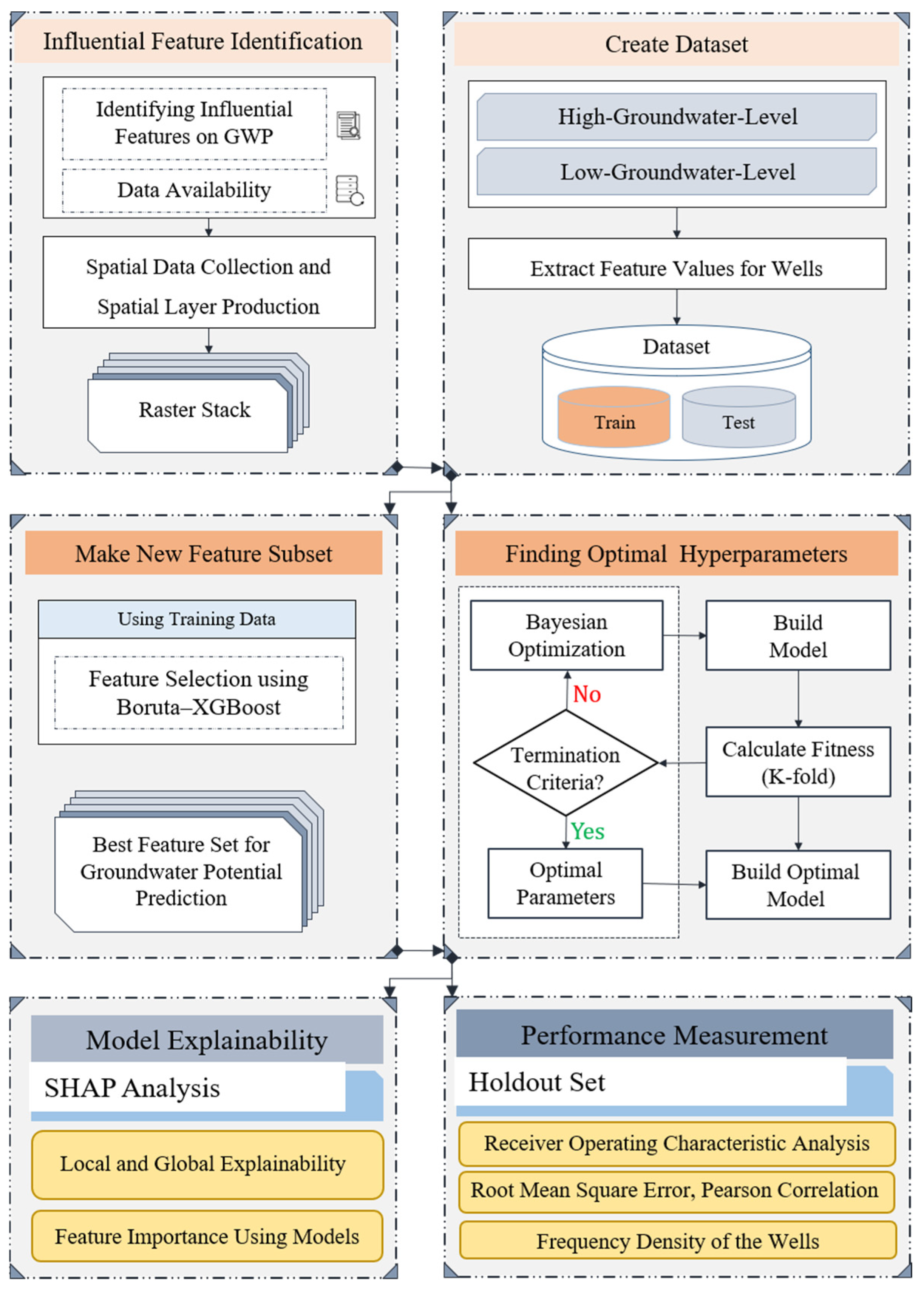
3.1. Proposed Methodology

Figure 3 demonstrates the methodology of this study, which consists of six main steps. First, based on the previous studies and data availability, relevant environmental features were collected and preprocessed. Then, using appropriate spatial analyses, the spatial layers of the identified features were prepared. To prepare the dataset, an inventory map of groundwater potential was prepared (1490 wells in the study area with high- and low-potential levels) and their features were extracted based on their spatial layers. Then, the prepared dataset was divided into training and testing datasets (80% for training and 20% for testing). Next, the Boruta–XGBoost algorithm was applied for feature selection to identify the most significant features influencing groundwater potential. Following this, the RF and CatBoost ML models were developed and optimized using a BOA to predict groundwater potential across the study area. RFs and CatBoost as two ML models illustrated competitive performance in the various application and achieved robust performances [29,30]. RF as a well-known ensemble ML model, rather than the other decision tree models, can handle outlier and noisy data, consequently providing more reliable decisions, as well as being able to effectively handle the overfitting issues in the decision tree-based models [74]. CatBoost, a new ensemble ML model, performs effectively on datasets with categorical features, a key attribute of the model [75]. In the optimizing models, the training dataset was based on a 10-fold cross validation divided into 9-fold for training and 1-fold for validation. The models were evaluated using performance metrics, including the RMSE, accuracy, sensitivity, specificity, precision, and AUC, to assess their accuracy and compare model performance. Also, some statistical information was calculated to assess the generalizability of the models. Finally, SHAP values were used to interpret the models and understand the contribution of each feature to the predictions, providing insights into the factors driving groundwater potential in the study area. In addition, the importance of these selected features was then evaluated using both the RF and CatBoost models and the Boruta–XGBoost algorithm.

3.2. Models

3.2.1. RFs

RFs are a powerful ML model used for classification and regression [76]. They build multiple decision trees during training, with each tree learning from a random subset of data and features. This randomness helps reduce overfitting and improves the model’s ability to handle unseen data [73]. RFs use a technique called bagging, where different feature subsets are used to create each tree, and each tree makes its own prediction [28]. The final result is obtained by combining all tree predictions.

More specifically, RFs consist of multiple tree-based predictors, represented as $h\left(x;{\theta }_k\right),$ where $k=1,\dots ,K$. Here, $x$ is the input data, and ${\theta }_k$ comprises randomly chosen subsets of the original dataset, each used to train a tree. At each decision point within a tree, a few random features are considered, and the one with the lowest Gini index is chosen to split the data. The Gini index is calculated for the variable $X_m$ with probability $P^i\left(i=1,2,\dots n\right)$ at node k by Equation (5) [28]:

$$Gini (X_m)=1-{{\displaystyle \sum }}_{i=1}^n{P_k^i}^2 ,$$

(5)

The final prediction is made by averaging the outputs of all trees.

3.2.2. CatBoost

CatBoost is a Gradient Boosting Decision Tree (GBDT) algorithm specifically designed to efficiently handle categorical features without requiring extensive preprocessing [77]. It improves upon traditional gradient boosting by sequentially constructing decision trees while minimizing errors based on the gradient of the loss function [78]. Unlike conventional GBDT methods, CatBoost integrates categorical feature processing directly into the training phase, enabling the model to leverage the entire dataset effectively [75].

During the training phase, CatBoost constructs decision trees sequentially, with each tree built to minimize loss and improve upon the previous predictions [79]. Since CatBoost is an improved version of GBDTs, understanding its mechanism begins with an overview of the GBDT algorithm. The GBDT model can be mathematically expressed as follows [41]:

$$F\left(x,w\right)={{\displaystyle \sum }}_{t=0}^T{a}_t{h}_t\left(x,w_t\right)={{\displaystyle \sum }}_{t=0}^T{f}_t\left(x,w_t\right),$$

(6)

where $F\left(x,w\right)$ represents the overall output, $x$ is the input sample, and $w$ denotes the model parameters. Here, $a_t$ is the weight at step $t$, $T$ is the total number of decision trees, $h_t\left(x,w_t\right)$ is the output of the $t$-th decision tree, and $f_t\left(x,w_t\right)$ represents the weighted output. Model optimization is achieved by minimizing the loss function [41]:

$$\left(a_t,w\right)=argmin {{\displaystyle \sum }}_{i=0}^{N}L\left(y_i,F\left(x_i,w\right)\right),$$

(7)

where $L$ denotes the loss function, typically measured using a mean squared error. Here, $y_i$ is the actual output, $x_i$ is the input sample, and $N$ represents the total number of samples.

CatBoost offers key advantages over traditional gradient boosting methods. First, it effectively manages categorical features by incorporating a prior value into the greedy target-based statistics approach, reducing conditional shift and improving performance [75]. Second, it integrates multiple categorical variables by merging features and their combinations within the current tree. Third, it addresses gradient bias through ordered boosting, which enhances generalization by reducing prediction shifts caused by biased gradient estimation [78,79].

3.3. Validation Criteria

To compare and evaluate models, two metrics were considered.

• Root Mean Square Error (RMSE)

The RMSE measures how well a model predicts data, with lower RMSE values indicating higher accuracy [26]. It is derived from the mean squared error (MSE), calculated as follows:

$$MSE={\displaystyle \frac{1}{n}}{{\displaystyle \sum }}_{i=1}^n{\left(y_i-{\widehat{y}}_i\right)}^2,$$

(8)

$$RMSE=\sqrt{MSE},$$

(9)

Here, $y_i$ represents the actual values, ${\widehat{y}}_i$ denotes the predicted values, and $n$ is the total number of observations.

• Receiver Operating Characteristic (ROC)

The ROC curve visually represents the performance of a binary classification model by plotting the true positive rate (sensitivity) against the false positive rate (1—specificity) [16]. The AUC quantifies the model’s ability to distinguish between the two classes (e.g., existence and non-existence of piezometric wells or high potential of groundwater and low potential of ground water), with values ranging from 0.5 to 1, where higher values indicate better classification performance [34].

The key metrics are defined as follows:

$$Sensitivity={\displaystyle \frac{TP}{TP+FN}} ,$$

(10)

$$Specificity={\displaystyle \frac{TN}{FP+TN}} ,$$

(11)

where TP, FP, TN, and FN represent true positives, false positives, true negatives, and false negatives, while P and N denote the total number of positive and negative samples, respectively.

• Accuracy

Accuracy is one of the most straightforward evaluation metrics, representing the proportion of correctly classified predictions out of the total number of outputs.

$$Accuracy={\displaystyle \frac{TP}{TP+\mathrm{FP}+\mathrm{TN}+\mathrm{FN}}} ,$$

(12)

• Precision

Precision calculates the proportion of true positive predictions among all predictions that were predicted as positive.

$$Precision={\displaystyle \frac{TP}{TP+\mathrm{FP}}} ,$$

(13)

3.4. Boruta Algorithm

Among the different feature selection methods including filters, wrappers, and embedded algorithms, the Boruta algorithm was selected for this study due to its robustness and proven effectiveness in identifying all relevant features [80]. Boruta, particularly when integrated with XGBoost, has shown superior performance in various applications by accounting for feature interactions and reducing the risk of overlooking weak but important predictors [16,37,81]. This choice aligns with our objective to ensure a reliable and comprehensive feature selection process.

The Boruta algorithm is a feature selection method that enhances the RF algorithm introduced by [80], which identifies the most important features in a dataset. The main problem with RFs in feature selection is that the importance scores they assign to variables may not always be reliable, as they can be influenced by correlations between features and the randomness of individual trees [80]. Breiman initially assumed that the importance scores followed a normal distribution, allowing a simple Z-score to assess significance [76], but this assumption was later proven incorrect. To address this issue, the Boruta algorithm was developed, introducing additional randomness by creating shadow features—randomized copies of the original features with no real correlation to the target variable [80]. Although the main core of the Boruta algorithm was developed based on RFs, utilizing the eXtreme gradient boosting algorithm (XGBoost) enhances the performance of Boruta based on previous studies [37,81]. Additionally, XGBoost tends to offer stable and robust feature importance rankings due to its gradient boosting framework and regularization capabilities, which help mitigate overfitting and overemphasis on noisy features.

XGBoost is a highly efficient and powerful ML algorithm designed for predictive tasks, developed as an advanced form of gradient boosting [82]. It constructs an ensemble of weak learners—typically decision trees—by sequentially minimizing a loss function $l$, which quantifies prediction errors. To prevent overfitting, XGBoost incorporates a regularization term $\Omega \left(f_t\right)$ into the loss function, striking a balance between model accuracy and complexity [83]. At each iteration t, a new tree $f_t\left(x_i\right)$ is added to the model as follows:

$$ℒ\left(t\right)={{\displaystyle \sum }}_{i=1}^{n}l(y_i, {\widehat{y}}_i^{\left(t-1\right)})+f_t\left(x_i\right)+\Omega \left(f_t\right),$$

(14)

To determine the Z-score, the feature importance of XGBoost should be calculated after training the XGBoost model on real and shadow features. Feature importance in XGBoost is determined by the gains of the leaf nodes before and after the split [83]. Gain shows the improvement in loss function by splits on a feature. In the next step, Z-scores for both real and shadow features are computed as follows:

$$Z-Score={\displaystyle \frac{\overline{G}}{\sigma }},$$

(15)

where $\overline{G}$ and $\sigma$ are the average value and standard variance of the gains at each tree [80,83]. After determining the Z-score for all features, those that exceed the Z-score of the most important shadow features are important and those below are non-important features. By comparing the importance of real features against these shadow features over multiple iterations of XGBoost, Boruta determines which features are truly significant. This ensures a more robust feature selection process, filtering out irrelevant features while retaining the most predictive ones [37].

3.5. Explainable Model (SHapley Additive exPlanation)

SHAP is a method that helps explain how ML models make predictions, which was introduced by [39]. Many advanced models, like deep learning and ensemble methods, are highly accurate but difficult to understand. SHAP solves this by assigning an importance score to each feature in a prediction, showing how much it contributed to the final result [45]. It is based on Shapley values from game theory, ensuring a fair distribution of contributions among features [44]. SHAP also unifies several existing explanation methods and improves their reliability and efficiency. This makes it a powerful tool for understanding complex models in a clear and consistent way [39].

4. Results

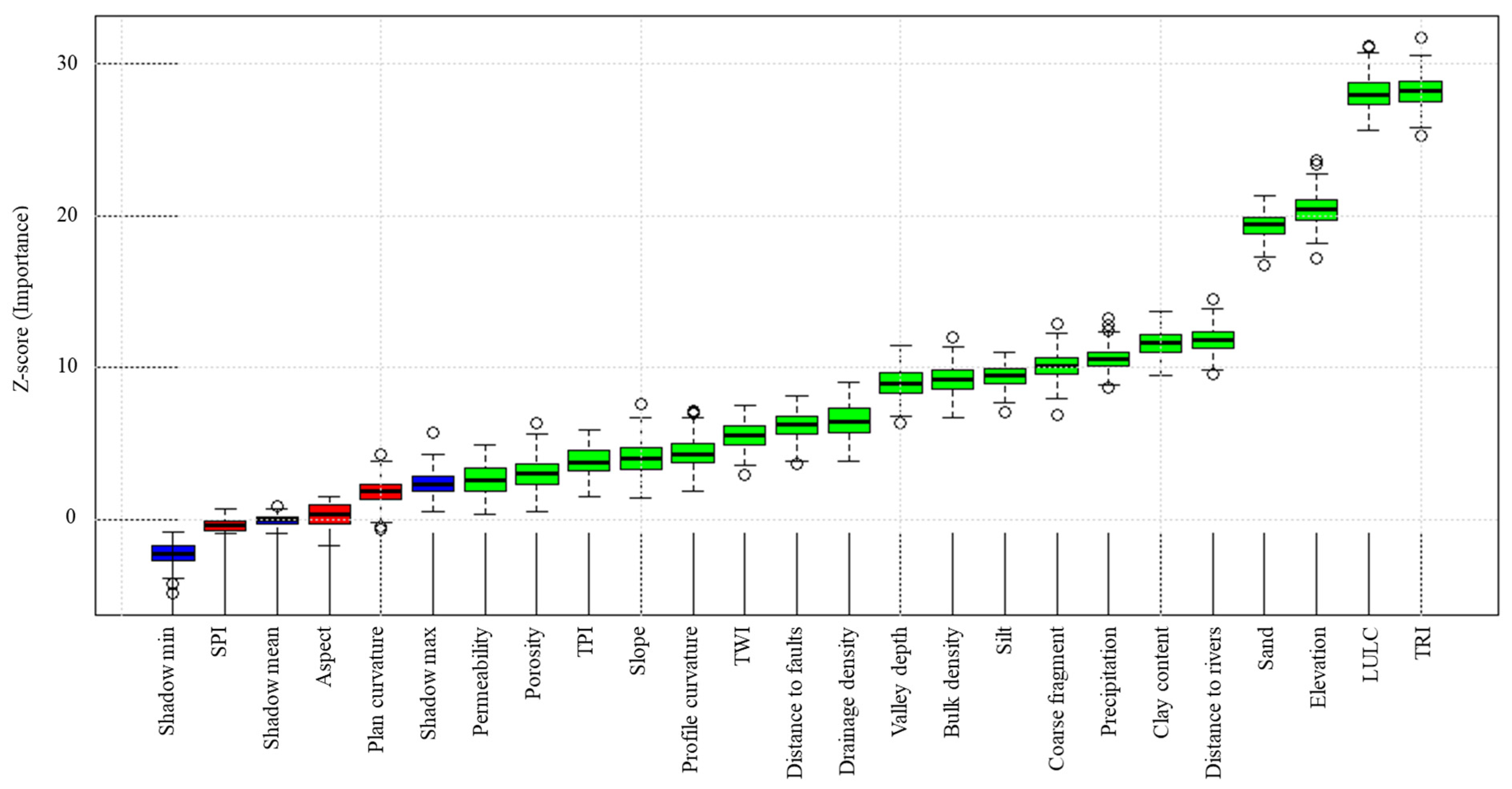
4.1. Feature Selection

To enhance the accuracy and robustness of models, the Boruta-XGBoost algorithm was utilized for feature selection. Initially, 22 features were considered and fed into ML models, but after feature selection, three features including the SPI, aspect, and plan curvature were eliminated from the rest of the processing (Figure 4). The features labeled as Min, Mean, and Max in Figure 4 are artificial shadow features generated by the Boruta algorithm. These are used as a baseline to assess the importance of real features and are not actual input variables. ShadowMin, the minimum importance of shadow features, acts as a threshold. A feature is considered unimportant if its importance is less than ShadowMin. ShadowMax, the maximum importance of shadow features, acts as a threshold. A feature is considered important if its importance is greater than ShadowMax. ShadowMean, the average importance of shadow features, indicates the performance of actual features relative to shadow features. An actual feature is considered important if its importance exceeds ShadowMean.

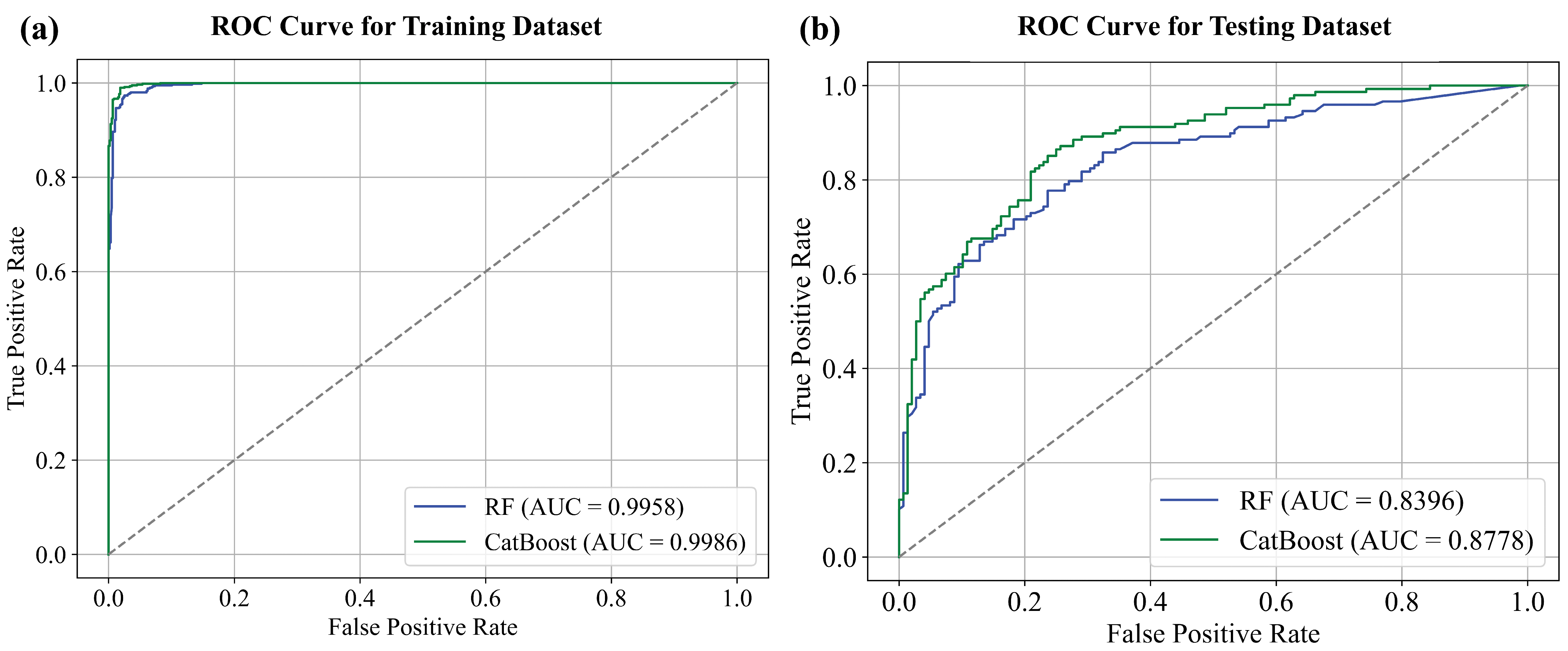
4.2. Model Development

Both the RF and CatBoost models were implemented in Python version 3.9 using the Jupyter Notebook within the base Anaconda environment. The dataset was divided into training and testing subsets, with 70% of the data used for training and the remaining 30% reserved for testing.

To optimize the performance of both models, hyperparameter tuning was performed using the Optuna library, a powerful framework for automated hyperparameter optimization. Optuna employs a Bayesian optimization approach to efficiently search the hyperparameter space and identify the best combination of parameters for each model (https://optuna.org/, accessed on 12 May 2025). The tuned hyperparameters for RFs and CatBoost are summarized in

Table 3. Hyperparameter ranges and optimized values for Random Forest and CatBoost models using Bayesian optimization.

Model	Hyperparameter	Type	Range	Optimized Value
RF	Number of trees	Integer	10 to 500	10
	Depth of trees	Integer	1 to 20	10
	Minimum samples to split a node	Integer	2 to 20	2
	Minimum samples at a leaf node	Integer	1 to 20	1
	Maximum features	String	[“sqrt”, “log2”, none]	None
CatBoost	Number of iterations	Integer	10 to 1000	500
	Learning rate	Float	0.01 to 0.2	0.026
	Depth	Integer	1 to 10	8
	L2 regularization	Float	1 to 9	8.258
	Random strength	Float	0.1 to 2.0	0.445
	Early stopping	Integer	10 to 100	50

.

The performance of both models was evaluated using the RMSE, AUC, accuracy, sensitivity, specificity, and precision metrics for both the training and testing datasets.

Table 4. Evaluation criteria for RFs and CatBoost in training and testing phases.

Training	RMSE	AUC	Accuracy	Sensitivity	Specificity	Precision
RF	0.2029	0.9957	0.9741	0.9748	0.9733	0.9732
CatBoost	0.2069	0.9986	0.9855	0.9815	0.9900	0.9898
Testing	RMSE	AUC	Accuracy	Sensitivity	Specificity	Precision
RF	0.4072	0.8396	0.7703	0.7635	0.7770	0.7740
CatBoost	0.3779	0.8778	0.8074	0.7500	0.8449	0.8473

and Figure 5 present the evaluation criteria and ROC curves in the training and testing phases, respectively.

According to Table 4, the RF model achieved a low RMSE of 0.2029, a high AUC of 0.9957, an accuracy of 0.9741, and a precision of 0.9732 on the training dataset. Similarly, the CatBoost model performed exceptionally well on the training dataset, with an RMSE of 0.2069, an AUC of 0.9986, an accuracy of 0.9855, and a precision of 0.9898 slightly outperforming the RF model in terms of all metrics except the RMSE.

On the testing dataset, the RF model achieved an RMSE of 0.4072, an AUC of 0.8396, an accuracy of 0.7703, and a precision of 0.7740. While the model’s performance decreased compared to the training set, it demonstrated good generalization capability. The CatBoost model outperformed the RF model on the testing dataset, with a lower RMSE of 0.3779, a higher AUC of 0.8778, a higher accuracy of 0.8074, and a higher precision of 0.8473. This indicates that the CatBoost model generalizes better to unseen data compared to the RF model.

Overall, both models showed a slight decrease in performance from the training to the testing dataset, which is expected. However, the drop in performance is moderate, suggesting that both models are well regularized and not significantly overfitting the training data. The CatBoost model consistently outperformed the RF model in both training and testing. The relatively low RMSE and high AUC, accuracy, and precision values on the testing dataset indicate that both models generalize well to unseen data, with CatBoost showing slightly better performance.

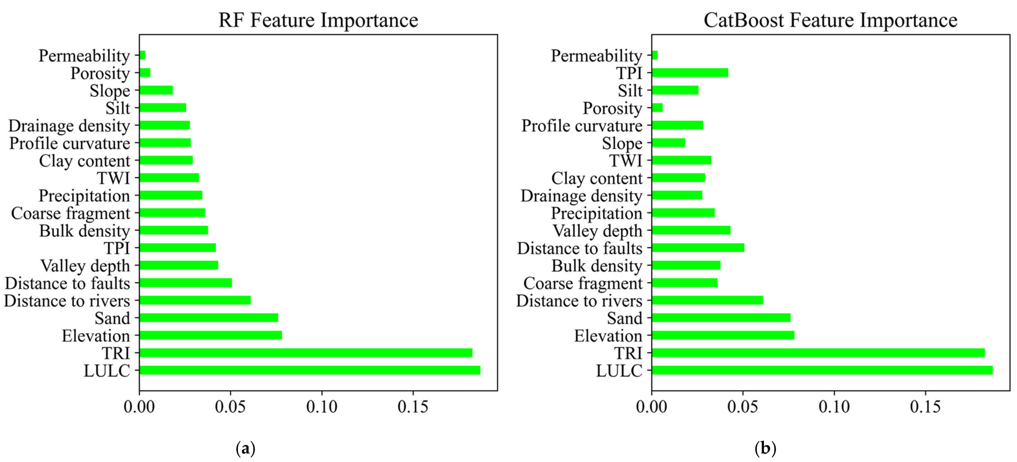
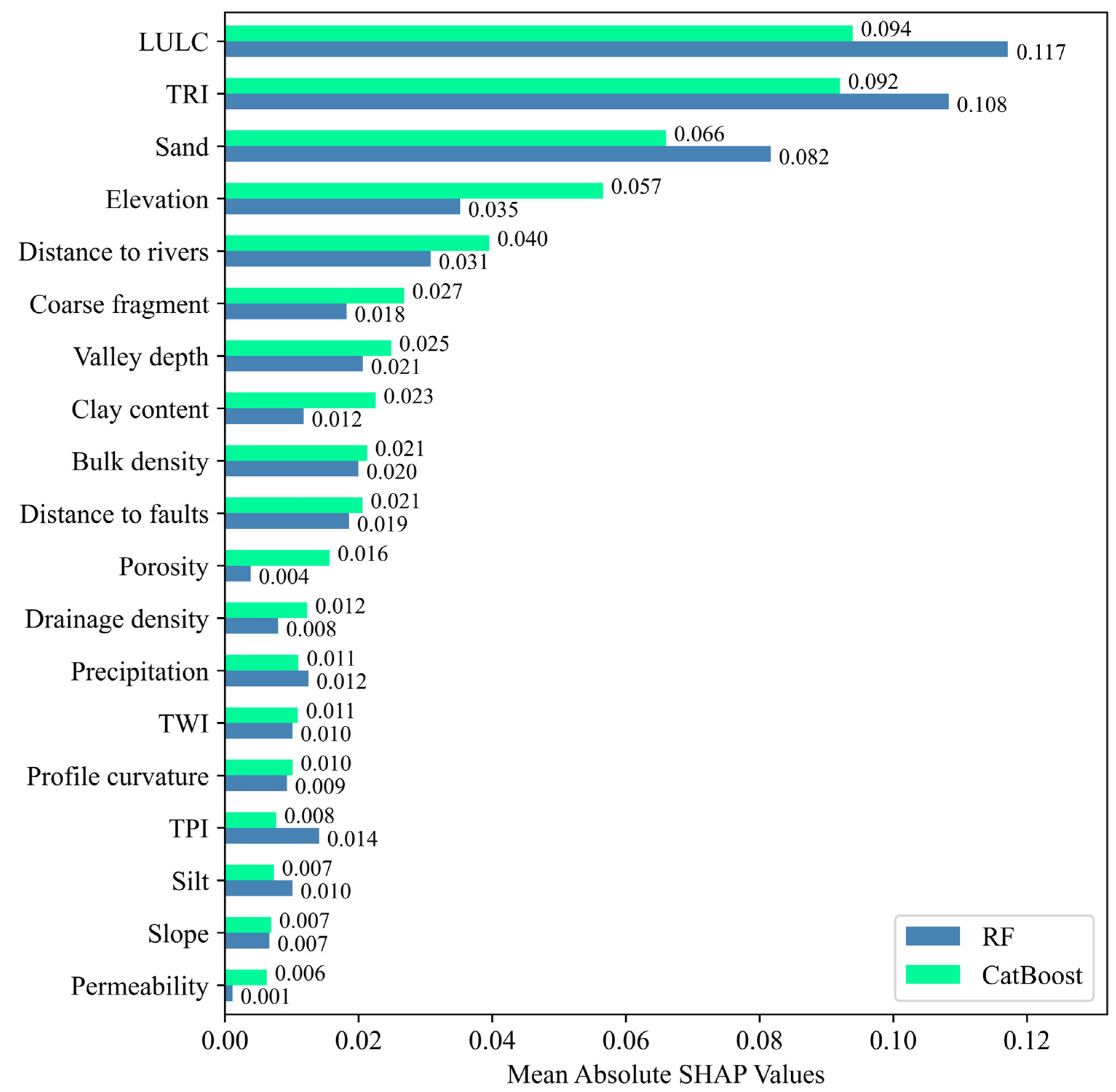
4.3. Feature Importance

The feature importance analysis for both the RF and CatBoost models revealed key insights into the features influencing groundwater potential. Figure 6 illustrates the relative importance of each feature used in the models.

For the RF model, the most important features by far were LULC and the TRI, with LULC having the highest importance score. These features were followed by elevation, sand, and the distance to rivers, which contributed to the model’s predictions but not as much as LULC and the TRI. On the other hand, the least important features in the RF model included permeability and porosity, which had relatively low importance.

In the CatBoost model, the feature importance ranking was slightly different but relatively followed a similar trend. The most influential features were LULC, the TRI, elevation, and sand, with LULC again emerging as the most critical parameter. The distance to rivers also played a significant role in the CatBoost model’s predictions. Conversely, the least important features in the CatBoost model were permeability, the TPI, and silt, which had minimal impact on the model’s predictions.

Overall, both models highlighted LULC, the TRI, and elevation as the most crucial parameters for predicting groundwater potential, while permeability, porosity, and silt were consistently among the least important parameters. This suggests that LULC, the TRI, and elevation are more influential in determining groundwater potential compared to soil properties such as permeability and porosity.

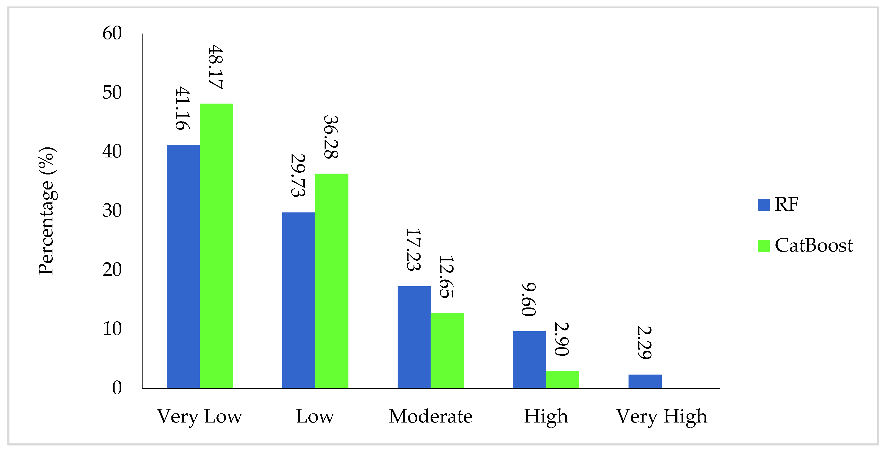
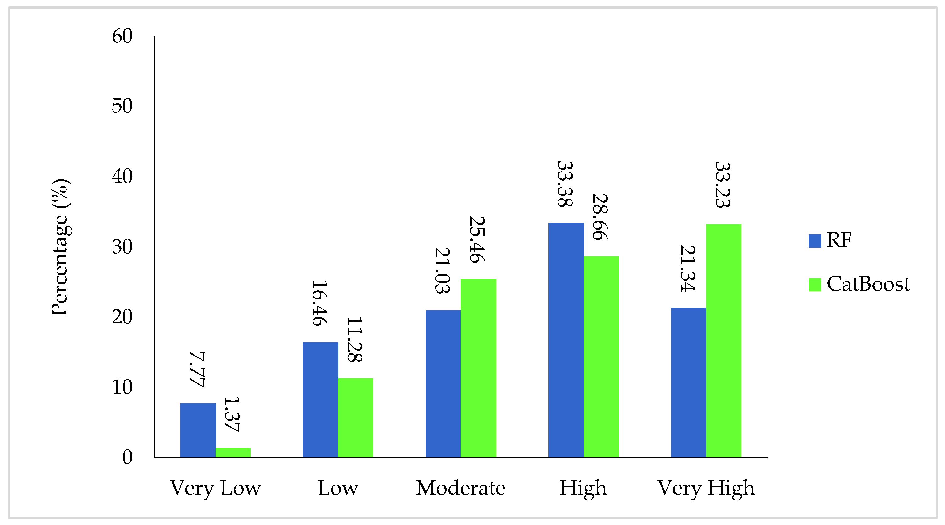
4.4. Groundwater Potential Maps

After training models, GWPMs were generated for the entire study area (Figure 7). These maps were divided into five categories (very high, high, moderate, low, and very low) using the natural break reclassification method in ArcGIS 10.8. Figure 8 shows the percentage of each category for both models. The RF model predicted that 35% and 29% of the study area fall under the very-high- and high-groundwater-potential categories, while 11% and 9% of the area are classified as low and very low, respectively. The moderate categories account for 16%. The CatBoost model predicted that 25% and 31% of the study area fall under the very-high- and high-groundwater-potential categories, respectively. Meanwhile, the percentages for the low and very low categories are 15% and 9%, respectively. The moderate category accounts for 20% of the area.

To further analyze the performance of the models, the distribution of class zero and class one points in each category of GWPMs was examined. According to Figure 9, the RF and CatBoost models assigned a significant portion of class zero points to the very low (48.17% and 41.16%) and low (36.28% and 29.73%) categories, respectively, which is expected since these categories represent areas with lower groundwater potential. The RF model assigned a small percentage of class zero points to the high (9.60%) and very high (2.29%) categories, while the CatBoost model assigned almost no points to these categories (2.90% for high and 0.00% for very high).

Based on Figure 10, the RF model assigned a higher percentage of class one points to the high category (33.38%) compared to the CatBoost model (28.66%). However, the CatBoost model assigned a much higher percentage of class one points to the very high category (33.23%) compared to the RF model (21.34%). The CatBoost model assigned fewer class one points to the very low (1.37%) and low (11.28%) categories compared to the RF model with 7.77% and 16.46%, respectively.

Overall, the CatBoost model is more effective at concentrating class zero points in very low and low categories, while the RF model shows a slightly broader distribution across all categories. Similarly, the CatBoost model is more effective at concentrating class one points in the very high category, whereas the RF model distributes these points more broadly across the high and very high categories. This indicates that CatBoost is more precise in distinguishing between areas of low and very high groundwater potential.

4.5. Model Interpretation

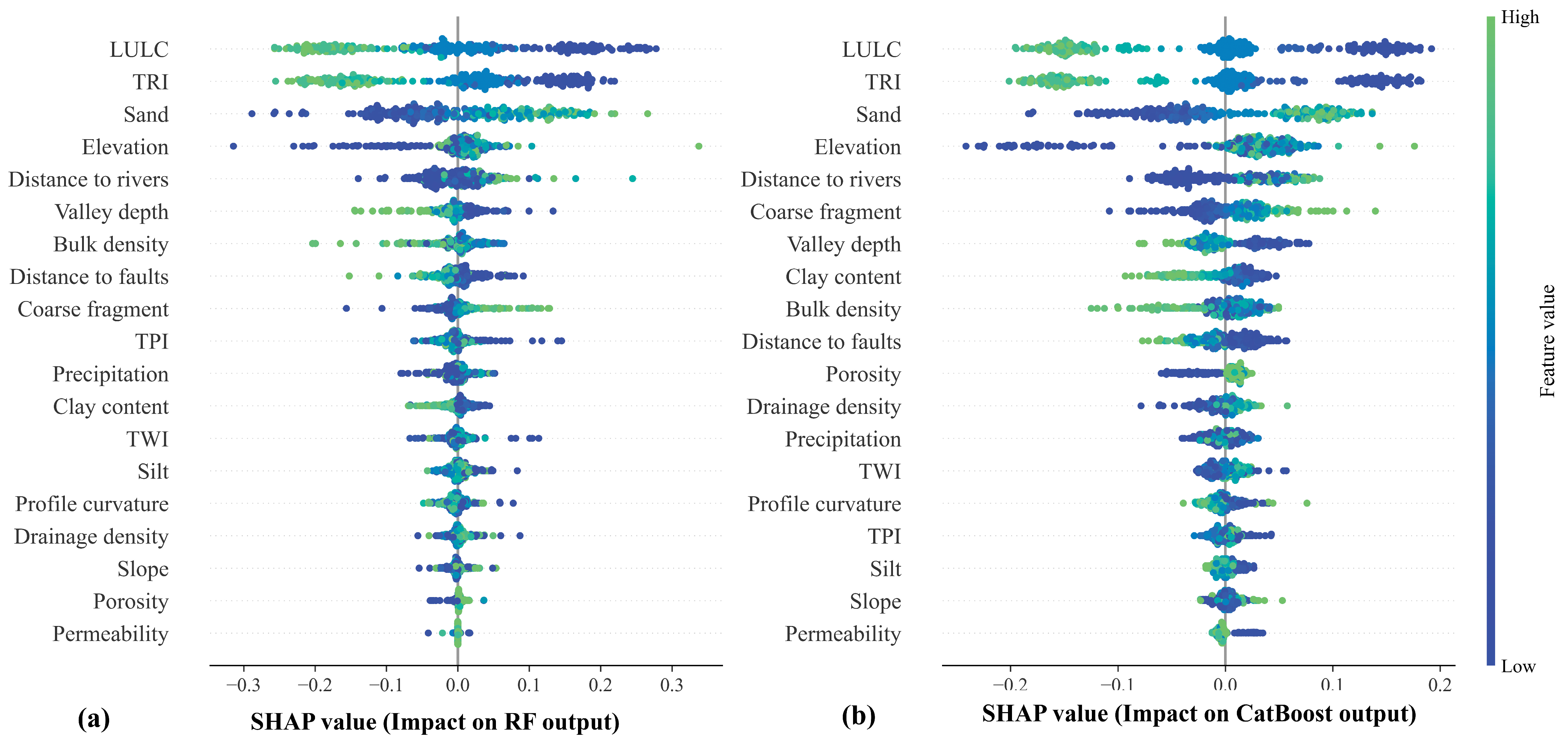
In this part, the contributions of features into the CatBoost model output were discussed globally and locally, as CatBoost was the superior model.

4.5.1. Global SHAP

Another way to interpret the predictions and outputs of models is through SHAP plots. Figure 11 demonstrates the impact of each feature on the output of the RF and CatBoost models. The SHAP values for both models range from −0.3 to 0.3, indicating the direction and magnitude of each feature’s influence on the model’s predictions.

For the RF model (Figure 11a), the SHAP values reveal that LULC and the TRI have the highest impact on the model’s output. LULC shows the widest range of SHAP values, indicating that it is the most influential feature. Higher values of LULC tend to have a negative impact on groundwater potential predictions, while lower values have a positive impact. The TRI also has a significant influence, with higher values generally contributing negatively to the model’s predictions. Features such as sand, elevation, and the distance to rivers also contribute to the model’s output but with relatively smaller SHAP values compared to LULC and the TRI. On the other hand, parameters like permeability, porosity, and slopes have minimum impact, as indicated by their near-zero SHAP values.

For the CatBoost model (Figure 11b), the SHAP values show a similar trend but with some differences in feature importance. LULC and TRI again emerge as the most influential features, with higher values negatively impacting the model’s predictions. Sand and elevation also show significant contributions, with higher values of these features generally leading to higher groundwater potential predictions and vice versa. The distance to rivers and coarse fragments have moderate impacts, with their SHAP values indicating that they contribute to the model’s output but to a lesser extent than LULC and the TRI. Features such as permeability, slopes, and silt have minimum impact, as reflected by their low SHAP values.

As illustrated in Figure 12, overall, the SHAP plots confirm that LULC, the TRI, sand, and elevation are the most influential parameters in both models, with LULC being the dominant parameters. This suggests that LULC and the TRI are the key drivers of groundwater potential, while some soil properties like permeability and porosity have a relatively minor impact. The consistency in feature importance across both models strengthens the reliability of these findings.

4.5.2. Local SHAP

One of the strengths of SHAP model explainability is its ability to demonstrate the contribution of each feature to the groundwater potential maps across the entire study area. The spatial distribution of SHAP values for each feature is presented in Figure 13.

According to Figure 13, high values of LULC and the TRI had a negative impact on the model’s output, while low values of elevation and sand positively influenced the model. For example, the southern and southwestern regions of Fars province, which are plain areas, show positive SHAP values in Figure 13d. Conversely, the northeastern part of the study area, characterized by low sand content, negatively influenced the groundwater potential map. Additionally, high values of LULC in the southern and eastern regions exhibited a negative influence (Figure 13a), while low values of LULC in the central and northern regions showed a positive impact on the groundwater potential map.

5. Discussion

This study utilized an interpretable approach to developing a groundwater potential map with the aim of enhancing the performance of ML models. By focusing on the feature selection, hyperparameter tunning, and interpretability of ML models, this approach addresses all aspects of groundwater potential prediction. It involves spatial feature extraction using spatial analysis, feature selection, the hyperparameter optimization of ML models, model performance evaluation using evaluation criteria, a generalization assessment based on statistical well data in the groundwater potential mapping, and, finally, the local and global interpretability of the models using SHAP analysis.

Data and features play a crucial role in ML models as the accuracy of input data determines their success or failure. Therefore, this study aimed to utilize both open national and global data. It is notable that influencing features on groundwater potential are both numerical and categorical data. Unlike previous studies [16,23,25] that relied on categorical soil and geology data, this study employed numerical layers of soil and geology. Additionally, the categorical LULC data were converted into numerical layers using the WoE method, ensuring consistency across all layers by converting them into a numerical format.

Although the importance of features can be directly extracted from the two decision tree-based models, RFs and CatBoost, their rankings have been shown to be inconsistent [84]. Therefore, the Boruta–XGBoost algorithm was employed to identify the most influential features influencing groundwater potential. As a result, the plan curvature, SPI, and aspect were removed as redundant features. According to the Boruta–XGBoost algorithm, the TRI, LULC, and elevation were identified as the most important features, while permeability, porosity, and the TPI were deemed the least significant. Similarly, feature importance rankings derived from the trained RF and CatBoost models indicated that LULC, the TRI, and elevation were the most influential features in both models. Conversely, permeability, porosity, and slopes were identified as the least important in the RF model, whereas permeability, porosity, and silt were the least significant in the CatBoost model.

The identification of key features based on the Boruta–XGBoost algorithm and decision tree-based models provides a global perspective. To further enrich the model interpretation, SHAP analysis was employed. SHAP values are computed by solving the prediction equation for each mapping unit. Therefore, instead of obtaining a general overview of feature importance, SHAP values reveal how each feature influences the groundwater potential for each mapping unit. Unlike other methods, SHAP allows for the calculation of the individual feature contributions for each mapping unit, which can then be visualized as spatial maps. These SHAP-based maps illustrate the contribution of each feature across the entire study area, providing a more detailed and interpretable representation of feature importance. According to the SHAP results for both models, LULC, the TRI, and sand were identified as the most influential features, while permeability was the least significant. Overall, both models consistently highlighted LULC and the TRI as the most critical features for groundwater potential prediction, whereas permeability remained among the least important parameters. This finding suggests that land use and terrain roughness have a greater impact on groundwater potential than geological characteristics such as permeability and porosity. These results align with the study by Sadeghi et al. [16] which identified precipitation and LULC as the most influential features. Similarly, Fatah et al. [26] recognized the TRI and slope as the key determinants of groundwater potential. While our study confirms the importance of the TRI, slopes exhibited low significance across the different methods in our analysis.

Both Boruta and SHAP consistently highlighted LULC and the TRI as the most influential features in determining groundwater potential. In the Boruta–XGBoost process, features such as permeability, porosity, and the TPI were among the least important. This was confirmed in the SHAP summary plots where these features showed near-zero SHAP values in both the RF and CatBoost models. As a result, the SHAP analysis validated the feature selection made by Boruta.

Although the SHAP results show that both models have similar trends in identifying the most and least important features, they have different feature importance rankings. This variability occurs because each algorithm has distinct internal mechanisms for learning patterns and interactions, leading to differences in feature prioritization.

Our findings indicate that the CatBoost model outperformed the RF model in the test dataset, with RMSE and AUC values of 0.3779 and 0.8778, respectively. Additionally, the predicted groundwater potential map aligns well with actual data. Specifically, the CatBoost and RF models classified 84.45% and 70.89% of wells with zero potential into the low and very low classes, respectively. The CatBoost and RF models identified 61.89% and 54.72% of wells with high potential in the high and very high classes. Thus, both models demonstrated reasonable generalization capability. However, the CatBoost model was more effective in concentrating class zero points in very low and low categories, whereas the RF model distributed them more broadly across different classes. Similarly, CatBoost was better at concentrating class one points in the very high category, whereas the RF model spread them between the high and very high categories. This indicates that CatBoost is more precise in distinguishing between areas of low and very high groundwater potential. Nevertheless, both models outperformed Sadeghi et al. [16], who found that 40% of wells with one potential were in the high and very high classes for the vision transformer and convolutional neural network models, respectively, while 69% and 77% of wells with zero potential were in the low and very low classes.

The results demonstrate that the CatBoost model outperformed the RF model. Similar trends have been observed in previous studies. Xiong et al. showed that CatBoost (AUC = 0.900) and XGBoost (AUC = 0.899) outperformed RFs (AUC = 0.75) [29]. Another study focusing on groundwater storage prediction also found CatBoost (AUC = 0.94) to outperform RFs (AUC = 0.89), supporting our findings [31]. In contrast, Nguyen et al. reported the slightly better performance for RFs (AUC = 0.99) compared to CatBoost (AUC = 0.98) [30].

This study employed ensemble ML models (RF and CatBoost) to model groundwater potential, leveraging their efficiency and inherent resistance to overfitting, a common issue in conventional ML algorithms. Unlike the CNN and VIT approaches used in previous research (e.g., Sadeghi et al. [16]), which are more susceptible to overfitting, RFs’ and CatBoost’s ensemble nature offers superior overfitting prevention, even compared to methods relying on hyperparameter optimization and feature selection (e.g., AlAyyash et al. [25]). Furthermore, the “no free lunch” theorem dictates that no single method universally solves every problem [85]. Therefore, this study explored and evaluated various ML methods, particularly ensemble approaches, to model groundwater potential in Fars province, Iran, assessing their effectiveness within this specific application.

Despite the reasonable accuracy of both models in identifying wells with potential one in the high and very high classes and those with potential zero in the low and very low classes, there are still some misclassification percentages. Additionally, there are variations in the selection of the most influential features for groundwater potential in the literature. Therefore, future research should focus on exploring different feature selection methods and developing more advanced models with higher reliability. Furthermore, in this study, in addition to local and global explainability, SHAP values were calculated for mapping units and a spatial pattern map of SHAP values was prepared for the entire study area. This study calculated and mapped the importance of each feature in predicting the groundwater potential for each 100 m × 100 m pixel. This provided a spatially explicit understanding of feature importance, unlike previous studies like Sadeghi et al. [16], which only assessed feature importance based on the ML training and testing data. However, to increase the explainability of ML models, it is suggested that different explainability strategies be used in future research. While a finer pixel size (e.g., 10, 30, or 85 m) could enhance accuracy and reduce uncertainty, the data in this study were prepared at 100 m resolution. Future work should compare these results with groundwater levels derived from satellite imagery to improve understanding of groundwater potential and assess the proposed approach’s performance. Furthermore, the impact of LULC change, land surface temperature, and climate change on groundwater potential represents a crucial area for future research not addressed here.

6. Conclusions

This study predicts groundwater potential in Fars province, Iran, using a Boruta–XGBoost algorithm for feature selection and Bayesian optimization to fine-tune RF and CatBoost models. SHAP values were used to enhance model interpretability. The results indicate that CatBoost outperformed RFs, achieving superior RMSE and AUC scores. The CatBoost model predicts that 25% and 31% of the study area have very high and high groundwater potential, respectively, while 15% and 9% have low and very low potential, respectively. The moderate category covers 20% of the area. These findings and the proposed approach offer valuable insights for groundwater management and informed decision-making in Fars province. This study recommends that decision-makers restrict the establishment of new wells in low- and very-low-potential areas and manage water extraction from existing wells. In these areas, the groundwater potential map advises against planting water-intensive and non-strategic crops. Furthermore, groundwater recharge programs and aquifer restoration should be prioritized. The proposed groundwater potential mapping approach can be applied to other regions to inform groundwater management and conservation planning.

References

1. UN Water (Ed.) The United Nations World Water Development Report 2022: Groundwater: Making the Invisible Visible; United Nations Educational, Scientific and Cultural Organization: Paris, France, 2022; ISBN 92-3-100507-3. [Google Scholar]
2. Díaz-Alcaide, S.; Martínez-Santos, P. Review: Advances in Groundwater Potential Mapping. Hydrogeol. J. 2019, 27, 2307–2324. [Google Scholar] [CrossRef]
3. Gleeson, T.; Befus, K.M.; Jasechko, S.; Luijendijk, E.; Cardenas, M.B. The Global Volume and Distribution of Modern Groundwater. Nat. Geosci. 2016, 9, 161–167. [Google Scholar] [CrossRef]
4. UN Water (Ed.) Water for Prosperity and Peace; The United Nations World Water Development Report; UNESCO: Paris, France, 2024; ISBN 978-92-3-100657-9. [Google Scholar]
5. Nugroho, J.T.; Lestari, A.I.; Gustiandi, B.; Sofan, P.; Prasasti, I.; Rahmi, K.I.N.; Noviar, H.; Sari, N.M.; Manalu, R.J.; Arifin, S. Groundwater Potential Mapping Using Machine Learning Approach in West Java, Indonesia. Groundw. Sustain. Dev. 2024, 27, 101382. [Google Scholar] [CrossRef]
6. UNESCO (Ed.) Nature-Based Solutions for Water; The United Nations world water development report; Unesco: Paris, France, 2018; ISBN 978-92-3-100264-9. [Google Scholar]
7. Wada, Y.; Flörke, M.; Hanasaki, N.; Eisner, S.; Fischer, G.; Tramberend, S.; Satoh, Y.; Van Vliet, M.; Yillia, P.; Ringler, C. Modeling Global Water Use for the 21st Century: The Water Futures and Solutions (WFaS) Initiative and Its Approaches. Geosci. Model. Dev. 2016, 9, 175–222. [Google Scholar] [CrossRef]
8. Noori, R.; Maghrebi, M.; Jessen, S.; Bateni, S.M.; Heggy, E.; Javadi, S.; Noury, M.; Pistre, S.; Abolfathi, S.; AghaKouchak, A. Decline in Iran’s Groundwater Recharge. Nat. Commun. 2023, 14, 6674. [Google Scholar] [CrossRef]
9. Mirzaei, A.; Saghafian, B.; Mirchi, A.; Madani, K. The Groundwater–energy–food Nexus in Iran’s Agricultural Sector: Implications for Water Security. Water 2019, 11, 1835. [Google Scholar] [CrossRef]
10. Safdari, Z. Groundwater Level Monitoring Across Iran’s Main Water Basins Using Temporal Satellite Gravity Solutions and Well Data. Ph.D. Thesis, Norwegian University of Science and Technology, Trondheim, Norway, 2021. [Google Scholar]
11. Maghrebi, M.; Noori, R.; Bhattarai, R.; Mundher Yaseen, Z.; Tang, Q.; Al-Ansari, N.; Danandeh Mehr, A.; Karbassi, A.; Omidvar, J.; Farnoush, H. Iran’s Agriculture in the Anthropocene. Earth’s Future 2020, 8, e2020EF001547. [Google Scholar] [CrossRef]
12. Samani, S. Analyzing the Groundwater Resources Sustainability Management Plan in Iran through Comparative Studies. Groundw. Sustain. Dev. 2021, 12, 100521. [Google Scholar] [CrossRef]
13. Safdari, Z.; Nahavandchi, H.; Joodaki, G. Estimation of Groundwater Depletion in Iran’s Catchments Using Well Data. Water 2022, 14, 131. [Google Scholar] [CrossRef]
14. Thanh, N.N.; Thunyawatcharakul, P.; Ngu, N.H.; Chotpantarat, S. Global Review of Groundwater Potential Models in the Last Decade: Parameters, Model Techniques, and Validation. J. Hydrol. 2022, 614, 128501. [Google Scholar] [CrossRef]
15. Noori, R.; Maghrebi, M.; Mirchi, A.; Tang, Q.; Bhattarai, R.; Sadegh, M.; Noury, M.; Torabi Haghighi, A.; Kløve, B.; Madani, K. Anthropogenic Depletion of Iran’s Aquifers. Proc. Natl. Acad. Sci. USA 2021, 118, e2024221118. [Google Scholar] [CrossRef]
16. Sadeghi, B.; Alesheikh, A.A.; Jafari, A.; Rezaie, F. Performance Evaluation of Convolutional Neural Network and Vision Transformer Models for Groundwater Potential Mapping. J. Hydrol. 2025, 654, 132840. [Google Scholar] [CrossRef]
17. Choudhary, S.; Jain, J.; Pingale, S.M.; Khare, D. A Comprehensive Review on Mapping of Groundwater Potential Zones: Past, Present and Future Recommendations. In Emerging Technologies for Water Supply, Conservation and Management; Springer: Berlin/Heidelberg, Germany, 2023; pp. 109–132. [Google Scholar]
18. Saranya, T.; Saravanan, S. Groundwater Potential Zone Mapping Using Analytical Hierarchy Process (AHP) and GIS for Kancheepuram District, Tamilnadu, India. Model. Earth Syst. Environ. 2020, 6, 1105–1122. [Google Scholar] [CrossRef]
19. Genjula, W.; Jothimani, M.; Gunalan, J.; Abebe, A. Applications of Statistical and AHP Models in Groundwater Potential Mapping in the Mensa River Catchment, Omo River Valley, Ethiopia. Model. Earth Syst. Environ. 2023, 9, 4057–4075. [Google Scholar] [CrossRef]
20. Adiat, K.; Nawawi, M.; Abdullah, K. Assessing the Accuracy of GIS-Based Elementary Multi Criteria Decision Analysis as a Spatial Prediction Tool–a Case of Predicting Potential Zones of Sustainable Groundwater Resources. J. Hydrol. 2012, 440, 75–89. [Google Scholar] [CrossRef]
21. Upadhyay, R.K.; Tripathi, G.; Đurin, B.; Šamanović, S.; Cetl, V.; Kishore, N.; Sharma, M.; Singh, S.K.; Kanga, S.; Wasim, M. Groundwater Potential Zone Mapping in the Ghaggar River Basin, North-West India, Using Integrated Remote Sensing and GIS Techniques. Water 2023, 15, 961. [Google Scholar] [CrossRef]
22. Ray, S. Unveiling Groundwater Gems: A GIS-Powered Fusion of AHP and TOPSIS for Mapping Groundwater Potential Zones. Groundw. Sustain. Dev. 2025, 29, 101431. [Google Scholar] [CrossRef]
23. Rana, M.S.P.; Rahman, M.T.; Hassan, M.F. Mapping Groundwater Potential Zone by Robust Machine Learning Algorithms & Remote Sensing Techniques in Agriculture Dominated Area, Bangladesh. Clean. Water 2025, 3, 100064. [Google Scholar]
24. Prapanchan, V.; Subramani, T.; Karunanidhi, D. GIS and Fuzzy Analytical Hierarchy Process to Delineate Groundwater Potential Zones in Southern Parts of India. Groundw. Sustain. Dev. 2024, 25, 101110. [Google Scholar] [CrossRef]
25. AlAyyash, S.; Al-Fugara, A.; Shatnawi, R.; Al-Shabeeb, A.R.; Al-Adamat, R.; Al-Amoush, H. Combination of Metaheuristic Optimization Algorithms and Machine Learning Methods for Groundwater Potential Mapping. Sustainability 2023, 15, 2499. [Google Scholar] [CrossRef]
26. Fatah, K.K.; Mustafa, Y.T.; Hassan, I.O. Groundwater Potential Mapping in Arid and Semi-Arid Regions of Kurdistan Region of Iraq: A Geoinformatics-Based Machine Learning Approach. Groundw. Sustain. Dev. 2024, 27, 101337. [Google Scholar] [CrossRef]
27. Razavi-Termeh, S.V.; Sadeghi-Niaraki, A.; Abba, S.I.; Ali, F.; Choi, S.-M. Enhancing Spatial Prediction of Groundwater-Prone Areas through Optimization of a Boosting Algorithm with Bio-Inspired Metaheuristic Algorithms. Appl. Water Sci. 2024, 14, 1–25. [Google Scholar] [CrossRef]
28. Halder, K.; Srivastava, A.K.; Ghosh, A.; Nabik, R.; Pan, S.; Chatterjee, U.; Bisai, D.; Pal, S.C.; Zeng, W.; Ewert, F. Application of Bagging and Boosting Ensemble Machine Learning Techniques for Groundwater Potential Mapping in a Drought-Prone Agriculture Region of Eastern India. Environ. Sci. Eur. 2024, 36, 155. [Google Scholar] [CrossRef]
29. Xiong, H.; Guo, X.; Wang, Y.; Xiong, R.; Gui, X.; Hu, X.; Li, Y.; Qiu, Y.; Tan, J.; Ma, C. Spatial Prediction of Groundwater Potential by Various Novel Boosting-Based Ensemble Learning Models in Mountainous Areas. Geocarto Int. 2023, 38, 2274870. [Google Scholar] [CrossRef]
30. Nguyen, H.D.; Nguyen, Q.-H.; Dang, D.K.; Nguyen, T.G.; Truong, Q.H.; Nguyen, V.H.; Bretcan, P.; Șerban, G.; Bui, Q.-T.; Petrisor, A.-I. Integrated Machine Learning and Remote Sensing for Groundwater Potential Mapping in the Mekong Delta in Vietnam. Acta Geophys. 2024, 72, 4395–4413. [Google Scholar] [CrossRef]
31. Uddin, M.S.; Mitra, B.; Mahmud, K.; Rahman, S.M.; Chowdhury, S.; Rahman, M.M. An Ensemble Machine Learning Approach for Predicting Groundwater Storage for Sustainable Management of Water Resources. Groundw. Sustain. Dev. 2025, 29, 101417. [Google Scholar] [CrossRef]
32. Moghaddam, D.D.; Rahmati, O.; Panahi, M.; Tiefenbacher, J.; Darabi, H.; Haghizadeh, A.; Haghighi, A.T.; Nalivan, O.A.; Bui, D.T. The Effect of Sample Size on Different Machine Learning Models for Groundwater Potential Mapping in Mountain Bedrock Aquifers. Catena 2020, 187, 104421. [Google Scholar] [CrossRef]
33. Ngouokouo Tchikangoua, A.; Enyegue A Nyam, F.M.; Kouamou Njifen, S.R.; Teikeu, W.A.; Ndougsa Mbarga, T.; Perilli, N. Bivariate Statistical and Neural Network Models to Map Groundwater Potential Zones in Bafia Area (Central Cameroon). Model. Earth Syst. Environ. 2025, 11, 44. [Google Scholar] [CrossRef]
34. Masroor, M.; Sajjad, H.; Kumar, P.; Saha, T.K.; Rahaman, M.H.; Choudhari, P.; Kulimushi, L.C.; Pal, S.; Saito, O. Novel Ensemble Machine Learning Modeling Approach for Groundwater Potential Mapping in Parbhani District of Maharashtra, India. Water 2023, 15, 419. [Google Scholar] [CrossRef]
35. Roy, S.K.; Hasan, M.M.; Mondal, I.; Akhter, J.; Roy, S.K.; Talukder, S.; Islam, A.S.; Rahman, A.; Karuppannan, S. Empowered Machine Learning Algorithm to Identify Sustainable Groundwater Potential Zone Map in Jashore District, Bangladesh. Groundw. Sustain. Dev. 2024, 25, 101168. [Google Scholar] [CrossRef]
36. Jafari, A.; Alesheikh, A.A.; Rezaie, F.; Panahi, M.; Shahsavar, S.; Lee, M.-J.; Lee, S. Enhancing a Convolutional Neural Network Model for Land Subsidence Susceptibility Mapping Using Hybrid Meta-Heuristic Algorithms. Int. J. Coal Geol. 2023, 277, 104350. [Google Scholar] [CrossRef]
37. Yousefi, Z.; Alesheikh, A.A.; Jafari, A.; Torktatari, S.; Sharif, M. Stacking Ensemble Technique Using Optimized Machine Learning Models with Boruta–XGBoost Feature Selection for Landslide Susceptibility Mapping: A Case of Kermanshah Province, Iran. Information 2024, 15, 689. [Google Scholar] [CrossRef]
38. Dahal, A.; Lombardo, L. Explainable Artificial Intelligence in Geoscience: A Glimpse into the Future of Landslide Susceptibility Modeling. Comput. Geosci. 2023, 176, 105364. [Google Scholar] [CrossRef]
39. Lundberg, S.M.; Lee, S.-I. A Unified Approach to Interpreting Model Predictions. In Proceedings of the Advances in Neural Information Processing Systems, 31st Conference on Neural Information Processing Systems (NIPS 2017), Long Beach, CA, USA, 4–9 December 2017; Volume 30. Available online: https://proceedings.neurips.cc/paper_files/paper/2017/file/8a20a8621978632d76c43dfd28b67767-Paper.pdf (accessed on 12 May 2025).
40. Ribeiro, M.T.; Singh, S.; Guestrin, C. “Why Should I Trust You?”: Explaining the Predictions of Any Classifier. In Proceedings of the Proceedings of the 22nd ACM SIGKDD International Conference on Knowledge Discovery and Data Mining, San Francisco, CA, USA, 13–17 August 2016; ACM: New York, NY, USA, 2016; pp. 1135–1144. [Google Scholar]
41. Razavi-Termeh, S.V.; Sadeghi-Niaraki, A.; Yao, X.A.; Naqvi, R.A.; Choi, S.-M. Assessment of Noise Pollution-Prone Areas Using an Explainable Geospatial Artificial Intelligence Approach. J. Environ. Manag. 2024, 370, 122361. [Google Scholar] [CrossRef] [PubMed]
42. Alesheikh, A.A.; Chatrsimab, Z.; Rezaie, F.; Lee, S.; Jafari, A.; Panahi, M. Land Subsidence Susceptibility Mapping Based on InSAR and a Hybrid Machine Learning Approach. Egypt. J. Remote Sens. Space Sci. 2024, 27, 255–267. [Google Scholar] [CrossRef]
43. Teke, A.; Kavzoglu, T. Exploring the Decision-Making Process of Ensemble Learning Algorithms in Landslide Susceptibility Mapping: Insights from Local and Global eXplainable AI Analyses. Adv. Space Res. 2024, 74, 3765–3785. [Google Scholar] [CrossRef]
44. Wang, N.; Zhang, H.; Dahal, A.; Cheng, W.; Zhao, M.; Lombardo, L. On the Use of Explainable AI for Susceptibility Modeling: Examining the Spatial Pattern of SHAP Values. Geosci. Front. 2024, 15, 101800. [Google Scholar] [CrossRef]
45. Jafari, A.; Alesheikh, A.A.; Zandi, I.; Lotfata, A. Spatial Prediction of Human Brucellosis Susceptibility Using an Explainable Optimized Adaptive Neuro Fuzzy Inference System. Acta Trop. 2024, 260, 107483. [Google Scholar] [CrossRef]
46. Bahrami, A.; Bahrami, M.; Haghani, E. Groundwater Quality Assessment for Potable Using WQI and GIS Technology in the South of Iran. Sustain. Water Resour. Manag. 2024, 10, 177. [Google Scholar] [CrossRef]
47. Jamalimoghaddam, E.; Yazdani, S.; Salami, H.; Peykani, G. The Impact of Water Supply on Farming Systems: A Sustainability Assessment. Sustain. Prod. Consum. 2019, 17, 269–281. [Google Scholar] [CrossRef]
48. Nouri, M.; Homaee, M.; Pereira, L.S.; Bybordi, M. Water Management Dilemma in the Agricultural Sector of Iran: A Review Focusing on Water Governance. Agric. Water Manag. 2023, 288, 108480. [Google Scholar] [CrossRef]
49. Torabi Haghighi, A.; Abou Zaki, N.; Rossi, P.M.; Noori, R.; Hekmatzadeh, A.A.; Saremi, H.; Kløve, B. Unsustainability Syndrome—From Meteorological to Agricultural Drought in Arid and Semi-Arid Regions. Water 2020, 12, 838. [Google Scholar] [CrossRef]
50. Aghaei, Y.; Nazari-Sharabian, M.; Afzalimehr, H.; Karakouzian, M. Hydrogeochemical Assessment of Groundwater Quality and Suitability for Drinking and Agricultural Use. The Case Study of Fars Province, Iran. Eng. Technol. Appl. Sci. Res. 2023, 13, 10797–10807. [Google Scholar] [CrossRef]
51. Golian, M.; Saffarzadeh, A.; Katibeh, H.; Mahdad, M.; Saadat, H.; Khazaei, M.; Sametzadeh, E.; Ahmadi, A.; Sharifi Teshnizi, E.; Samadi Darafshani, M. Consequences of Groundwater Overexploitation on Land Subsidence in Fars Province of Iran and Its Mitigation Management Programme. Water Environ. J. 2021, 35, 975–985. [Google Scholar] [CrossRef]
52. Razavi-Termeh, S.V.; Sadeghi-Niaraki, A.; Farhangi, F.; Khiadani, M.; Pirasteh, S.; Choi, S.-M. Solving Water Scarcity Challenges in Arid Regions: A Novel Approach Employing Human-Based Meta-Heuristics and Machine Learning Algorithm for Groundwater Potential Mapping. Chemosphere 2024, 363, 142859. [Google Scholar] [CrossRef]
53. Nguyen, P.T.; Ha, D.H.; Jaafari, A.; Nguyen, H.D.; Van Phong, T.; Al-Ansari, N.; Prakash, I.; Le, H.V.; Pham, B.T. Groundwater Potential Mapping Combining Artificial Neural Network and Real AdaBoost Ensemble Technique: The DakNong Province Case-Study, Vietnam. Int. J. Environ. Res. Public Health 2020, 17, 2473. [Google Scholar] [CrossRef]
54. Bennett, G. Analysis of Methods Used to Validate Remote Sensing and GIS-Based Groundwater Potential Maps in the Last Two Decades: A Review. Geosystems Geoenvironment 2024, 3, 100245. [Google Scholar] [CrossRef]
55. Gleeson, T.; Moosdorf, N.; Hartmann, J.; van Beek, L. van A Glimpse beneath Earth’s Surface: GLobal HYdrogeology MaPS (GLHYMPS) of Permeability and Porosity. Geophys. Res. Lett. 2014, 41, 3891–3898. [Google Scholar] [CrossRef]
56. Gleeson, T. GLobal HYdrogeology MaPS (GLHYMPS) of Permeability and Porosity 2018 [Dataset]. [CrossRef]
57. Jaafarzadeh, M.S.; Tahmasebipour, N.; Haghizadeh, A.; Pourghasemi, H.R.; Rouhani, H. Groundwater Recharge Potential Zonation Using an Ensemble of Machine Learning and Bivariate Statistical Models. Sci. Rep. 2021, 11, 5587. [Google Scholar] [CrossRef]
58. Tebege, E.G.; Birara, Z.M.; Takele, S.G.; Jothimani, M. Geospatial Mapping and Multi-Criteria Analysis of Groundwater Potential in Libo Kemkem Watershed, Upper Blue Nile River Basin, Ethiopia. Sci. Afr. 2025, 27, e02549. [Google Scholar]
59. Rodriguez, M.M.C.; Ferolin, T.P. Groundwater Resource Exploration and Mapping Methods: A Review. J. Environ. Eng. Sci. 2023, 19, 140–156. [Google Scholar] [CrossRef]
60. Tahmassebipoor, N.; Rahmati, O.; Noormohamadi, F.; Lee, S. Spatial Analysis of Groundwater Potential Using Weights-of-Evidence and Evidential Belief Function Models and Remote Sensing. Arab. J. Geosci. 2016, 9, 1–18. [Google Scholar] [CrossRef]
61. Benjmel, K.; Amraoui, F.; Boutaleb, S.; Ouchchen, M.; Tahiri, A.; Touab, A. Mapping of Groundwater Potential Zones in Crystalline Terrain Using Remote Sensing, GIS Techniques, and Multicriteria Data Analysis (Case of the Ighrem Region, Western Anti-Atlas, Morocco). Water 2020, 12, 471. [Google Scholar] [CrossRef]
62. Mokarram, M.; Roshan, G.; Negahban, S. Landform Classification Using Topography Position Index (Case Study: Salt Dome of Korsia-Darab Plain, Iran). Model. Earth Syst. Environ. 2015, 1, 1–7. [Google Scholar] [CrossRef]
63. Yıldırım, Ü. Identification of Groundwater Potential Zones Using GIS and Multi-Criteria Decision-Making Techniques: A Case Study Upper Coruh River Basin (NE Turkey). ISPRS Int. J. Geo-Inf. 2021, 10, 396. [Google Scholar] [CrossRef]
64. El Sherbini, R.A.; Ghazala, H.H.; Ahmed, M.A.; Ibraheem, I.M.; Al Ajmi, H.F.; Genedi, M.A. Mapping Groundwater Potential Zones in the Widyan Basin, Al Qassim, KSA: Analytical Hierarchy Process-Based Analysis Using Senti-Nel-2, ASTER-DEM, and Conven-Tional Data. Remote Sens. 2025, 17, 766. [Google Scholar] [CrossRef]
65. Chen, W.; Wang, Z.; Wang, G.; Ning, Z.; Lian, B.; Li, S.; Tsangaratos, P.; Ilia, I.; Xue, W. Optimizing Rotation Forest-Based Decision Tree Algorithms for Groundwater Potential Mapping. Water 2023, 15, 2287. [Google Scholar] [CrossRef]
66. Riley, S.J.; DeGloria, S.D.; Elliot, R. Index That Quantifies Topographic Heterogeneity. Intermt. J. Sci. 1999, 5, 23–27. [Google Scholar]
67. Affum, A.O.; Kwaansa-Ansah, E.E.; Osae, S.D. Estimating Groundwater Geogenic Arsenic Contamination and the Affected Population of River Basins Underlain Mostly with Crystalline Rocks in Ghana. Environ. Chall. 2024, 15, 100898. [Google Scholar] [CrossRef]
68. Rahmati, O.; Nazari Samani, A.; Mahdavi, M.; Pourghasemi, H.R.; Zeinivand, H. Groundwater Potential Mapping at Kurdistan Region of Iran Using Analytic Hierarchy Process and GIS. Arab. J. Geosci. 2015, 8, 7059–7071. [Google Scholar] [CrossRef]
69. Song, Q.; Ma, M.; Liu, Y.; Wang, Z.; Wu, W.; Xu, Z.; Xue, J. Identifying Groundwater Potential Zones in a Typical Irrigation District Using the Geospatial Technique and Analytic Hierarchy Process. Geocarto Int. 2025, 40, 2453025. [Google Scholar] [CrossRef]
70. Taibou, A.; Jounaid, H.; Moustadraf, J.; Amraoui, F. Assessment of Groundwater Potential in the Khenifra-Azrou Basin, Central Massif, Morocco Using Frequency Ratio and Shannon’s Entropy Approaches. Sci. Afr. 2025, 27, e02616. [Google Scholar] [CrossRef]
71. Kumar, P.; Singh, P.; Asthana, H.; Yadav, B.; Mukherjee, S. Groundwater Potential Zone Mapping of Middle Andaman Using Multi-Criteria Decision-Making and Support Vector Machine. Groundw. Sustain. Dev. 2024, 26, 101191. [Google Scholar] [CrossRef]
72. Nguyen, T.G.; Phan, K.A.; Huynh, T.H.N. Application of Integrated-Weight Water Quality Index in Groundwater Quality Evaluation. Civ. Eng. J. 2022, 8, 2661–2674. [Google Scholar] [CrossRef]
73. Hasanuzzaman, M.; Mandal, M.H.; Hasnine, M.; Shit, P.K. Groundwater Potential Mapping Using Multi-Criteria Decision, Bivariate Statistic and Machine Learning Algorithms: Evidence from Chota Nagpur Plateau, India. Appl. Water Sci. 2022, 12, 58. [Google Scholar] [CrossRef]
74. Razavi-Termeh, S.V.; Pourzangbar, A.; Sadeghi-Niaraki, A.; Franca, M.J.; Choi, S.-M. Metaheuristic-Driven Enhancement of Categorical Boosting Algorithm for Flood-Prone Areas Mapping. Int. J. Appl. Earth Obs. Geoinf. 2025, 136, 104357. [Google Scholar] [CrossRef]
75. Razavi-Termeh, S.V.; Sadeghi-Niaraki, A.; Jelokhani-Niaraki, M.; Choi, S.-M. Exploring Multi-Pollution Variability in the Urban Environment: Geospatial AI-Driven Modeling of Air and Noise. Int. J. Digit. Earth 2024, 17, 2378819. [Google Scholar] [CrossRef]
76. Breiman, L. Random Forests. Mach. Learn. 2001, 45, 5–32. [Google Scholar] [CrossRef]
77. Prokhorenkova, L.; Gusev, G.; Vorobev, A.; Dorogush, A.V.; Gulin, A. CatBoost: Unbiased Boosting with Categorical Features. 2017. arXiv 2017, arXiv:1706.09516. [Google Scholar]
78. Bairami, M.; Khajavi, H.; Rastgoo, A. Assessing Groundwater Behavior and Future Trends in the Ardabil Aquifer: A Comparative Study of Groundwater Modeling System and Categorical Gradient Boosting Hybrid Model. Expert. Syst. Appl. 2024, 255, 124728. [Google Scholar] [CrossRef]
79. Chen, B.; Chen, Y.; Chen, H. An Interpretable CatBoost Model Guided by Spectral Morphological Features for the Inversion of Coastal Water Quality Parameters. Water 2024, 16, 3615. [Google Scholar] [CrossRef]
80. Kursa, M.B.; Jankowski, A.; Rudnicki, W.R. Boruta—A System for Feature Selection. Fundam. Informaticae 2010, 101, 271–285. [Google Scholar] [CrossRef]
81. Zandi, I.; Jafari, A.; Lotfata, A. Enhancing PM 2.5 Air Pollution Prediction Performance by Optimizing the Echo State Network (ESN) Deep Learning Model Using New Metaheuristic Algorithms. Urban. Sci. 2025, 9, 138. [Google Scholar] [CrossRef]
82. Ribeiro, M.T.; Singh, S.; Guestrin, C. A Scalable Tree Boosting System. In Proceedings of the 22nd ACM Sigkdd International Conference on Knowledge Discovery and Data Mining, San Francisco, CA, USA, 13–17 August 2016; pp. 785–794. [Google Scholar]
83. Yuan, X.; Chen, F.; Xia, Z.; Zhuang, L.; Jiao, K.; Peng, Z.; Wang, B.; Bucknall, R.; Yearwood, K.; Hou, Z. A Novel Feature Susceptibility Approach for a PEMFC Control System Based on an Improved XGBoost-Boruta Algorithm. Energy AI 2023, 12, 100229. [Google Scholar] [CrossRef]
84. Lundberg, S.M.; Erion, G.; Chen, H.; DeGrave, A.; Prutkin, J.M.; Nair, B.; Katz, R.; Himmelfarb, J.; Bansal, N.; Lee, S.-I. Explainable AI for Trees: From Local Explanations to Global Understanding. arXiv 2019, arXiv:1905.04610. [Google Scholar] [CrossRef]
85. Wolpert, D.H.; Macready, W.G. No free lunch theorems for optimization. IEEE Trans. Evol. Comput. 1997, 1, 67–82. [Google Scholar] [CrossRef]
Figure 1. Study area and spatial distribution of wells.
Water 17 01520 g001
Figure 2. Environmental features: (a) elevation, (b) slope, (c) aspect, (d) plan curvature, (e) profile curvature, (f) valley depth, (g) SPI, (h) TWI, (i) TPI, (j) TRI, (k) distance to faults, (l) permeability, (m) porosity, (n) drainage density, (o) distance to rivers, (p) precipitation, (q) bulk density, (r) clay content, (s) coarse fragments, (t) sand, (u) silt, and (v) LULC.
Water 17 01520 g002
Figure 3. The methodology framework.
Water 17 01520 g003
Figure 4. The determined features’ importance using the Boruta–XGBoost method.
Water 17 01520 g004
Figure 5. ROC curves using (a) training and (b) testing datasets.
Water 17 01520 g005
Figure 6. Feature importance of models: (a) RF and (b) CatBoost.
Water 17 01520 g006
Figure 7. GWMPs generated using (a) RF and (b) CatBoost models.
Water 17 01520 g007
Figure 8. Proportion of each category of GWMP generated using (a) RF and (b) CatBoost models.
Water 17 01520 g008
Figure 9. Percentage of class zero points in each category of GWPMs.
Water 17 01520 g009
Figure 10. Percentage of class one points in each category of GWPMs.
Water 17 01520 g010
Figure 11. Violin diagram of SHAP values for (a) RF and (b) CatBoost models.
Water 17 01520 g011
Figure 12. Mean absolute SHAP values for RF and CatBoost models.
Water 17 01520 g012
Figure 13. Spatial pattern of SHAP values for (a) LULC, (b) TRI, (c) sand, (d) elevation, (e) distance to rivers, (f) valley depth, (g) bulk density, (h) distance to faults, (i) coarse fragment, (j) TPI, (k) precipitation, (l) clay content, (m) TWI, (n) silt, (o) profile curvature, (p) drainage density, (q) slope, (r) porosity, (s) permeability.
Water 17 01520 g013