Advancing Ion Constituent Simulations in California’s Sacramento–San Joaquin Delta Using Machine Learning Tools

Abstract

This study extends previous machine learning work on ion constituent simulation in California’s Sacramento–San Joaquin Delta (Delta) to include three critical water intake locations. The developed Artificial Neural Network models demonstrate exceptional accuracy (R² > 0.96) in predicting chloride, bromide, and sulfate concentrations at these strategically important facilities. Water intake location models show substantial improvements in prediction accuracy, with MAE reductions of 60.7–74.0% for chloride, 63.3–72.5% for bromide, and 70.4–87.9% for sulfate, compared to existing methods for the Interior Delta. Performance evaluation through comprehensive cross-validation confirms robust model stability across varied conditions, with remarkably consistent metrics (standard deviation in R² ≤ 0.006). Four complementary interactive dashboards were developed, enabling users, regardless of programming expertise, to simulate ion constituents throughout the Delta system. A Model Interpretability Dashboard specifically addresses the complexity of machine learning models by visualizing parameter sensitivity and prediction behavior, thereby enhancing transparency and building stakeholder trust in the modeling approach. For the first time, spatial coverage limitations are addressed through hybrid modeling that combines DSM2 hydrodynamic simulation with machine learning to enable continuous prediction of ion distributions across several points in the Interior Delta. These advancements provide water managers with accessible, accurate tools for informed decision-making regarding agricultural operations, drinking water treatment, and ecosystem management in this vital water resource.

1. Introduction

The Sacramento–San Joaquin Delta (Delta) serves as California’s most crucial water hub, where the state’s two largest rivers, Sacramento River and San Joaquin River, converge to form a 2978-square-kilometer (1150-square-mile) inland Delta and estuary system [1,2]. This vital water resource supports approximately 27 million people, irrigates 1.21 million hectares of farmland, and maintains a diverse ecosystem of over 750 species [3,4]. Beyond water conveyance, the Delta generates significant economic value through recreation, recreational fishing, and transportation activities.

Water quality in the Delta, particularly the concentration levels of ion constituents including dissolved chloride, bromide, and sulfate, directly impacts multiple stakeholders and uses. For agricultural operations, elevated chloride levels can increase soil salinity and reduce crop yields. In urban water treatment, high bromide concentrations lead to the formation of harmful disinfection by-products (DBPs), requiring additional treatment steps to ensure public safety [5,6]. Agricultural runoff, urban development, and tidal influences continuously introduce various pollutants and ions into the system, making water quality monitoring and prediction essential for effective management [7,8,9].

Managing these water quality challenges requires balancing diverse needs: agricultural productivity, drinking water safety, and ecosystem health [10]. The complex interplay between these demands, combined with Delta’s dynamic hydrology, creates a pressing need for accurate and timely water quality monitoring and prediction tools [11].

Physical sampling and laboratory analysis remain the gold standard for monitoring ion constituents in the Delta, providing highly accurate and reliable measurements of water quality parameters [12]. This direct measurement approach ensures precise quantification of individual ion constituents and serves as the foundation for calibrating and validating other estimation methods.

However, traditional sampling methods present several limitations:

• Time and cost constraints: laboratory analysis often requires days or weeks to complete, involving substantial personnel and equipment resources.
• Limited coverage: physical sampling provides only point-in-time measurements at specific locations, lacking continuous temporal and spatial coverage.
• Operational delays: the time lag between collecting samples in the field and receiving laboratory results can impede timely operational decisions for water management.

These limitations have driven the development of alternative approaches for estimating ion constituent levels, particularly through the use of Electrical Conductivity (EC) as a proxy measurement.

Due to the limitations of direct sampling, scientists have explored faster and more cost-effective methods for estimating ion constituent levels in the Delta. Electrical Conductivity (EC) has emerged as a valuable proxy measurement, due to its unique advantages in water quality monitoring. EC can be measured continuously through in situ sensors and simulated effectively through hydrodynamic models, providing real-time monitoring capabilities that are crucial for operational decision-making [13]. Moreover, EC demonstrates strong correlations with various ion concentrations, making it a reliable indicator of the overall ionic content in water [14]. These characteristics have made EC the foundation for most ion constituent estimation methods in the Delta, enabling more frequent and widespread simulation than would be possible through direct sampling alone.

The development of methods for estimating ion constituents from EC measurements spans several decades. Classical approaches primarily rely on parametric regression equations, assuming that the relationship between EC and ion concentrations follows specific mathematical patterns (linear, quadratic, etc.) under different conditions [15,16,17]. These methods aim to simplify the conversion process from EC measurements to ion constituent levels.

The evolution of these approaches shows increasing sophistication over time. The pioneering work by [18] established the foundation by developing linear regression equations between EC, chloride, and total dissolved solids (TDS). Throughout the 1990s and early 2000s, researchers significantly expanded upon this foundation. Jung [19] investigated correlations between EC and various ions in Delta island return flows, while Suits [20] developed linear relationships between EC, chloride, and bromide at Delta export locations. A significant advancement came with Denton’s comprehensive study, which provided multiple methodological approaches for estimating a broader suite of ions [5].

The current state-of-the-art classical approach, developed by Hutton et al. [21], represents the most comprehensive parametric regression method to date. This study introduced a novel decision tree framework that determines appropriate regression equations based on multiple factors, including the sub-region of the Delta, Water Year Type (WYT), Month, and Sacramento X2 location [22], which is a key marker for salinity intrusion. Using these parameters, the method classifies conditions as seawater-dominated, San Joaquin River-dominated, or mixed, applying specific equations accordingly.

While the approach of Hutton et al. [21] significantly improved upon previous methods, it faces several limitations. A fundamental challenge lies in the simplified source assumptions, where classical methods generally consider only two major sources of salinity—seawater and the San Joaquin River. Agricultural drainage, despite being a significant salinity source in the Delta, is often oversimplified or considered aligned with the San Joaquin River source. This simplification can lead to inaccuracies, since agricultural drainage has distinct ionic compositions and behavior patterns compared to river inflows.

The handling of mixed conditions presents another significant challenge. Classical models tend to oversimplify these conditions by assuming a dominant source or using a single equation for mixed conditions. However, the reality is more complex, since salinity in the Delta typically results from multiple simultaneous sources, with their relative influences varying over time. The same EC level can correspond to markedly different ionic compositions depending on the source: seawater-dominated water often contains higher proportions of chloride and bromide, whereas water influenced by agricultural drainage or river flows is generally richer in sulfate.

Perhaps the most challenging aspect is the dynamic nature of these mixed conditions. The Delta exists almost perpetually in a mixed state, with salinity levels influenced by multiple sources simultaneously. The relationship between EC and ion concentrations shifts dynamically based on the varying contributions from different sources, and current parametric approaches struggle to capture these relationships, particularly during periods of rapid hydrological changes.

These limitations highlight the need for more sophisticated approaches that can better capture the complex and dynamic relationships between EC and ion constituents in the Delta system. Machine learning methods, with their ability to identify and adapt to complex patterns in data, offer promising solutions to these challenges.

Recent developments in machine learning have opened new possibilities for addressing these challenges. Following established protocols for water and environmental modeling using machine learning in California [23], our first study [24] served as a proof of concept to evaluate whether machine learning models could outperform traditional regression equations in simulating ion constituents. This pioneering work focused on the South Delta region, using a relatively small dataset of approximately 200 samples collected from seven stations between 2018 and 2020. Using R (https://www.r-project.org/, accessed on 1 June 2022) as the programming platform, we compared four machine learning approaches—Generalized Additive Model, Regression Trees, Random Forest, and Artificial Neural Networks—against conventional regression equations. The results demonstrated that machine learning models, particularly Random Forest, provided superior simulations of ion constituents compared to traditional regression equations. These improvements were especially notable for ions that exhibit pronounced non-linear relationships with EC. This study established the viability of machine learning approaches for simulating ion constituents in the Delta.

Building on these promising initial results, our subsequent research [25] significantly expanded both the geographic and temporal scope of the analysis. Implemented in Python (https://www.python.org/, accessed on 1 June 2022) this comprehensive study covered the entire Interior Delta and incorporated an extensive dataset spanning over 60 years, with sample sizes ranging from approximately 1000 to 2000 measurements for different ion constituents. This study developed and validated Artificial Neural Network (ANN) architectures specifically designed for ion constituent prediction, demonstrating remarkable improvements over the benchmark classical approach [21]. The ANN model showed significant improvements in both accuracy metrics, with R² improvements ranging from 0% for well-modeled constituents like TDS, to 85% for more complex constituents like sulfate. More importantly, the ANN model reduced the Mean Absolute Error (MAE) across all constituents, with improvements of 24% for TDS, 33% for magnesium, 32% for sodium, 40% for calcium, 34% for chloride, 59% for sulfate, 25% for bromide, 26% for alkalinity, and 20% for potassium. Additionally, the study introduced an interactive web browser-based dashboard hosted on Microsoft Azure, making these sophisticated prediction tools accessible to users regardless of their programming expertise. This user-friendly interface allows stakeholders to simulate ion levels under various hydrological conditions, compare results across different machine learning models, and visualize outcomes for informed decision-making.

The current study builds on the two studies mentioned above [24,25] and extends them in several important directions. First, we focus on applying ML models to three strategically important drinking water intake locations, where water quality monitoring is crucial for operational decision-making. Second, we enhance the accessibility and utility of our modeling tools through three complementary dashboards: (a) a new publicly available dashboard for intake locations; (b) an improved version of our previous dashboard [25] that incorporates Hutton et al.’s [22] parametric regression equations for direct comparison with ML approaches for the Interior Delta; and (c) a novel Model Interpretability Dashboard that helps demystify the “black box” nature of ML models by visualizing how they respond to different predictors and operating conditions for the Interior Delta. This third dashboard is particularly innovative as it allows users to explore model behavior, assess sensitivity to input variables, and build trust in ML predictions by comparing them with traditional parametric approaches. Finally, to address key limitations of current ML approaches—specifically, their temporal and spatial distribution constraints and inability to simulate potential future scenarios—we develop a novel hybrid water quality model that combines hydrodynamic modeling with machine learning, supported by its own interactive dashboard for scenario exploration and analysis. Together, these advancements not only provide more accurate predictions, but also make complex ML models more transparent and interpretable for water resource managers, helping them to make more informed decisions about monitoring and managing ion constituents in the Delta.

This paper first presents our development of machine learning models for predicting ion constituents (chloride, bromide, and sulfate) at three critical water intake locations. We describe our methodology, including data characteristics and model optimization procedures, followed by performance analyses demonstrating significant improvements over existing approaches.

We then present three complementary web-based tools. The first is a new Intake Locations Dashboard specifically designed for water intake locations. The other two dashboards build upon the previous Interior Delta study of Namadi et al. [25]: an Enhanced Comparison Dashboard that integrates classical methods with machine learning approaches, and a Model Interpretability Dashboard that helps users to understand model behavior across the Interior Delta.

To address spatial coverage limitations in the Interior Delta, we introduce a novel hybrid approach combining DSM2 hydrodynamic modeling with machine learning [26]. This model enables continuous spatial prediction of ion constituents across 162 points throughout the Interior Delta.

Finally, we discuss implications of the current study for Delta water management, acknowledge current limitations, and suggest directions for future research.

2. Materials and Methods

2.1. Study Area and Dataset Characteristics

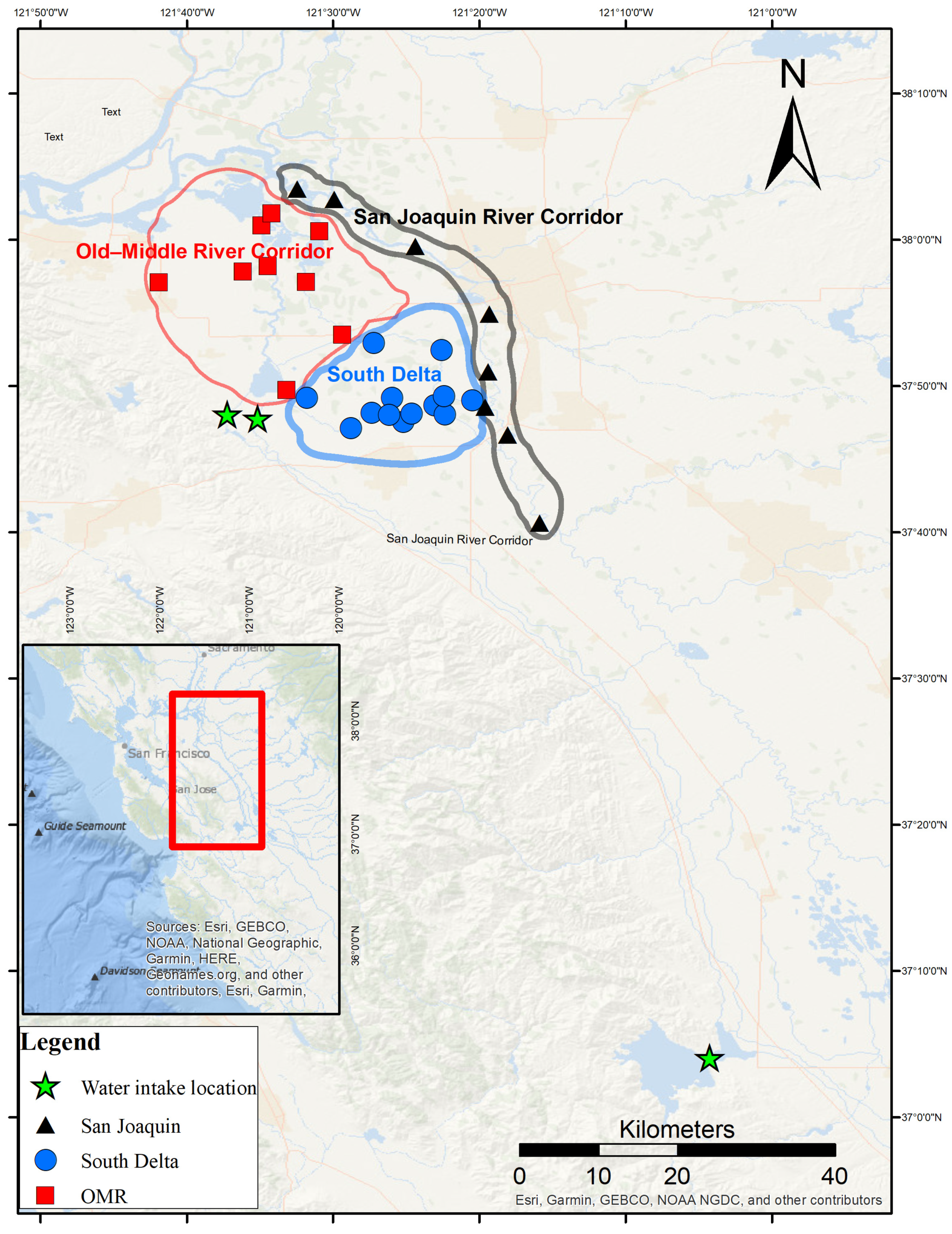
Our research synthesizes and builds upon two complementary datasets from the Delta: the Interior Delta dataset from our previous work [25] and a new focused dataset from strategic water intake locations. As shown in Figure 1, our study area encompasses both interior monitoring stations and critical water intake facilities. The Interior Delta monitoring network consists of three sub-regions: the Old and Middle River corridor (OMR, shown as red squares), the San Joaquin River corridor (SJRcorridor, marked by black triangles), and the South Delta region (represented by blue circles). The water intake locations, depicted as green stars, include three strategically important pumping plants: the Harvey O. Banks Pumping Plant (HRO; 37°47′53″ N, 121°37′23″ W), the Tracy Pumping Plant (TRP; 37°48′00″ N, 121°35′06″ W), and the O’Neill Forebay at the Gianelli Pumping Plant (ONG; 37°03′60″ N, 121°04′19″ W).

This study encompasses two complementary analyses. First, we expand upon our previous work that developed machine learning models for nine ion constituents (TDS, magnesium, sodium, calcium, chloride, sulfate, bromide, alkalinity, and potassium) across the Interior Delta monitoring stations, providing enhanced analysis and interpretation through our new dashboard tools. Second, we extend our modeling approach to water intake locations, where available monitoring data focus on three key ion constituents (chloride, bromide, and sulfate). These three constituents are particularly crucial for water quality management at pumping facilities, as they directly impact treatment processes and water supply operations.

The temporal and spatial coverage of these datasets reveals distinct characteristics that reflect their different roles in Delta water management. The Interior Delta dataset encompasses data from 1959 to 2022, though the temporal coverage varies by constituent and location. For detailed information about the Interior Delta monitoring timeline and data characteristics, readers are referred to our previous study [25]. In contrast, our water intake locations feature more recent but substantially more intensive monitoring programs. The HRO and TRP data collection spans from 2019 to 2023, while ONG has a longer record, from 2012 to 2023. These locations are characterized by high-frequency sampling, resulting in robust sample sizes: ONG collected 2620–2783 samples, while HRO and TRP gathered 1214–1328 and 1181–1233 samples, respectively. This intensive monitoring reflects the operational importance of these facilities in California’s water supply infrastructure.

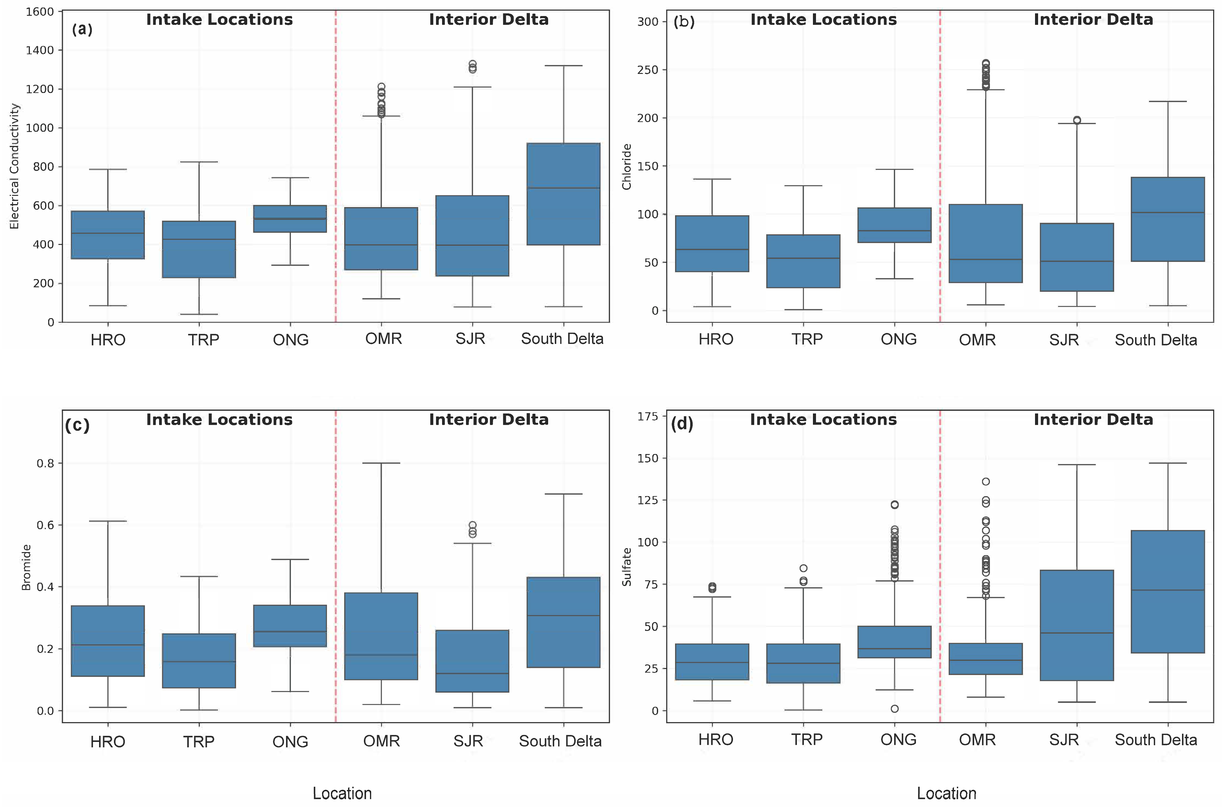
Analysis of constituent distributions, as illustrated in Figure 2, reveals distinct patterns between the Interior Delta and the water intake locations. Interior Delta locations consistently show higher variability and maximum values across all the measured constituents. The South Delta region exhibits the highest median EC values and widest range, varying from approximately 200 to 1400 μS/cm, while intake locations maintain more consistent EC patterns between 300 and 800 μS/cm. Similar patterns emerge for chloride concentrations, where Interior Delta locations, particularly the South Delta and OMR, show notably higher maximum values and greater variability compared to the more stable concentrations at intake locations.

Bromide distributions follow comparable trends, with OMR exhibiting particularly high outliers and greater variability compared to the relatively consistent levels maintained at intake locations. Sulfate concentrations in the Interior Delta, especially in the South Delta and SJRcorridor, show higher median values and greater variability compared to intake locations, though ONG typically shows slightly higher median values among the intake locations, while still maintaining more stable concentrations overall.

These distinct patterns between the Interior Delta and the intake locations reflect their different roles in the Delta system. The Interior Delta locations capture the system’s natural variability and multiple water source influences, resulting in wider ranges of constituent concentrations. The more consistent patterns at intake locations reflect managed operations and water quality control measures, which are crucial for maintaining reliable water supply quality.

This comparison provides crucial context for our modeling approach and dashboard development. The stark differences between the Interior Delta and intake locations—particularly in sampling frequency (moderate vs. intensive) and constituent variability (wide-ranging vs. more consistent)—reveal fundamentally different water quality patterns at these locations. Due to these distinct characteristics, we developed separate simulation models specifically for water intake locations, rather than applying our Interior Delta models. This location-specific modeling approach ensures that predictions accurately reflect the unique water quality dynamics and operational patterns at each type of monitoring site.

2.2. Model Development

2.2.1. Input Variable Selection

Our model development utilized a consistent set of predictor variables across both Interior Delta and water intake locations, maintaining methodological continuity with our previous work [25]. The selected predictors capture key physical and operational factors influencing ion constituent concentrations:

1. Electrical Conductivity (EC): A real-time measurement obtained through in situ sensors that indicates the water’s ability to conduct an electrical current, serving as a proxy for total dissolved solids and overall salinity levels [27]. EC measurements provide continuous monitoring capabilities, which are crucial for operational decision-making.

2. Sacramento X2: A key hydrodynamic indicator, measured as the distance (in kilometers) from the Golden Gate Bridge to the location where the tidally averaged near-bottom salinity is 2 practical salinity units (psu) [28]. This metric effectively captures Delta outflow conditions and the extent of seawater intrusion from the Pacific Ocean into the Delta system [29].

3. Water Year Type (WYT): California’s water year runs from October 1 to September 30, with types classified as Wet, Above-Normal, Below-Normal, Dry, or Critical, based on measured unimpaired runoff [30]. This classification integrates various hydrological factors, including precipitation, snowmelt, and river flows, providing a comprehensive indicator of water availability and system conditions [31].

4. Month: This is included to capture seasonal patterns in water quality, reflecting cyclical changes in precipitation, temperature, agricultural practices, and water management operations.

5. Location: A categorical variable distinguishing between monitoring sites. For water intake locations, this includes HRO, TRP, and ONG, while the Interior Delta locations are categorized into the OMR, SJRcorridor, and South Delta sub-regions.

These predictors were selected for their demonstrated relationships with ion constituent concentrations and their operational relevance in water management. The combination of continuous (EC, X2) and categorical (WYT, Location, and Month) variables enables our models to capture both direct relationships and complex interaction effects influencing water quality patterns.

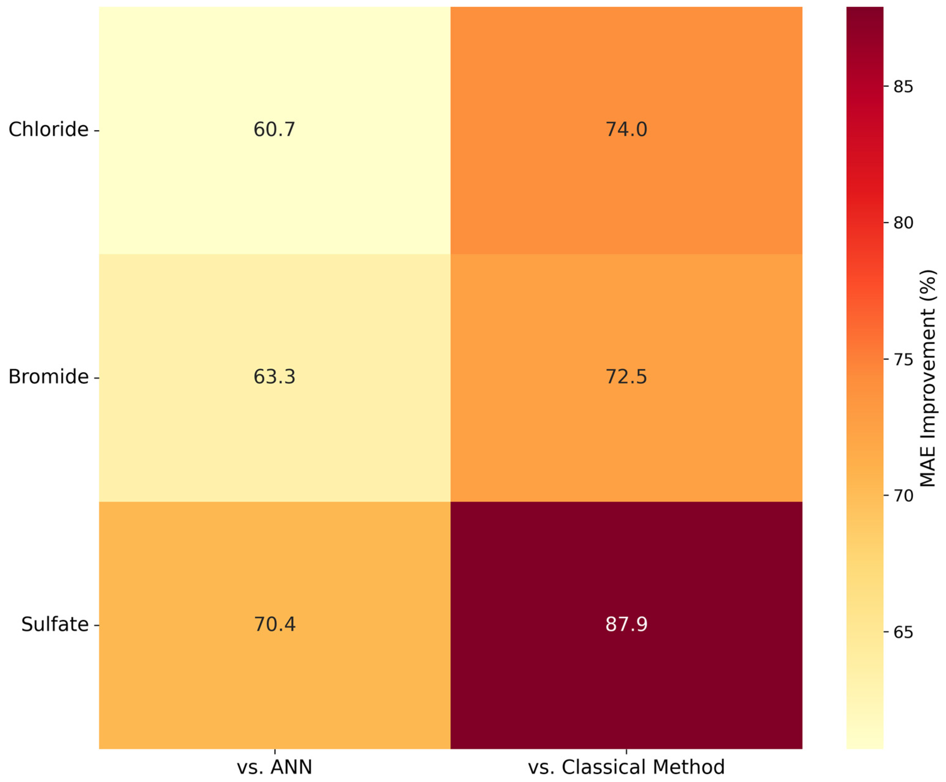
While maintaining methodological consistency, our benchmark comparison uses performance metrics from existing approaches. Since no prior models exist for water intake locations, we compared our new models’ performance metrics against the documented performance of both ML and classical methods in the Interior Delta [24,25]. For example, if the Interior Delta ML model demonstrated a specific MAE for chloride predictions in that region, we used this as a benchmark to evaluate our new model’s MAE for chloride predictions at water intake locations. This comparison, while across different locations, provides context for assessing our models’ relative performance in predicting ion constituents.

Data preprocessing and quality control were crucial steps to ensure model reliability. We implemented a regression-based outlier detection method focusing on the fundamental relationship between EC and ion constituents, where points exceeding three standard deviations from the regression line were flagged as potential outliers. This analysis revealed minimal outliers across locations, as detailed in

Table 1. Summary of outlier analysis and regression relationships between EC and ion constituents at water intake locations.

Location	Constituent	Total Samples	Outliers (%)	R2	Regression Equation
HRO	Chloride	1328	0.1	0.93	Cl = 0.19 × EC − 20.2
HRO	Bromide	1214	1.1	0.78	Br = 0.0007 × EC − 0.1
HRO	Sulfate	1328	0	0.53	SO4 = 0.06 × EC + 2.2
ONG	Chloride	2665	0.1	0.69	Cl = 0.22 × EC − 28.9
ONG	Bromide	2620	0.4	0.57	Br = 0.0007 × EC − 0.1
ONG	Sulfate	2783	1.3	0.33	SO4 = 0.08 × EC − 3.4
TRP	Chloride	1227	2.8	0.82	Cl = 0.16 × EC − 11.7
TRP	Bromide	1181	1.4	0.67	Br = 0.0006 × EC − 0.05
TRP	Sulfate	1233	0.6	0.58	SO4 = 0.06 × EC + 2.5

, with outlier percentages generally less than 3% across all constituents and locations. The strong coefficient of determination (R²) values, particularly for chloride (0.928 at HRO, 0.688 at ONG, and 0.823 at TRP), indicated high data quality and validated our outlier detection approach. Figure 3 illustrates the relationship between EC and chloride concentrations at the three water intake locations, demonstrating both the effectiveness of our outlier detection method and the varying relationships at different locations.

Following outlier detection, we implemented a comprehensive feature preprocessing pipeline using Scikit-learn’s ColumnTransformer function to prepare the data for model training. Numerical predictors (EC and X2) were standardized using the StandardScaler function to transform them to zero mean and unit variance, ensuring consistent scale across features and preventing convergence issues during model training. Categorical variables (Location, WYT, Month) were transformed using one-hot encoding to convert them into binary features while avoiding multicollinearity. This preprocessing pipeline was saved using joblib to ensure consistent transformation of future data points. The standardization and encoding approach helps to prevent any single feature from dominating the model training process, ensures proper handling of categorical information, and facilitates stable model convergence during training.

2.2.2. Machine Learning Approaches

Machine learning, a subset of artificial intelligence, enables computers to learn patterns from data without explicit programming [32]. In recent years, machine learning techniques have been increasingly applied to water quality modeling, due to their ability to capture complex, non-linear relationships in environmental systems. Numerous studies have demonstrated the effectiveness of machine learning in water quality applications, including the prediction of dissolved oxygen [33], suspended sediment [34], and salinity [35,36,37,38].

Artificial Neural Networks (ANNs) are particularly powerful machine learning models inspired by biological neural networks [39]. Among the various ANN architectures, we employed the Multi-Layer Perceptron (MLP), a feedforward neural network architecture well suited for regression problems like ion constituent prediction. The MLP architecture consists of multiple layers of interconnected nodes (neurons), with each connection having an associated weight that is adjusted during training. Each neuron applies a non-linear activation function to the weighted sum of its inputs, enabling the network to learn complex patterns in the data. This architecture has proven effective in various water quality applications, including prediction of chemical oxygen demand and analysis of heavy metal content.

Building upon our previous comparative analysis of machine learning algorithms [25], we employed ANNs for simulating ion constituent concentrations at water intake locations. The selection of ANNs was guided by their demonstrated superior performance in capturing non-linear relationships between environmental predictors and ion concentrations in the Delta system, particularly their ability to adapt to complex spatial and temporal patterns in water quality dynamics. We implemented an MLP architecture using TensorFlow [40]. The model training utilized the Adam optimizer with the mean squared error (MSE) loss function, chosen for its effectiveness in regression tasks and adaptability to varying gradients.

Hyperparameter optimization is a crucial step in developing neural networks, as these parameters significantly influence model performance, but cannot be learned directly from training data. Unlike model weights and biases that are updated during training, hyperparameters must be set before the training process begins. However, the complex interactions between different hyperparameters make it challenging to determine their optimal values theoretically, necessitating empirical optimization approaches.

MLPs have a number of hyperparameters, including network architecture (number of layers and neurons), activation functions, learning rate, batch size, optimizer settings, and regularization parameters. Optimizing all possible hyperparameters simultaneously would be computationally intensive and often impractical. For instance, considering just five options for ten hyperparameters would result in 5¹⁰ (approximately 9.7 million) possible combinations. Therefore, researchers typically focus on optimizing a subset of hyperparameters that are known to have the most significant impact on model performance.

In this study, we focused on three critical hyperparameters:

• Number of hidden layers (2 to 5 layers);
• Number of neurons per layer (10, 20, 30, or 40);
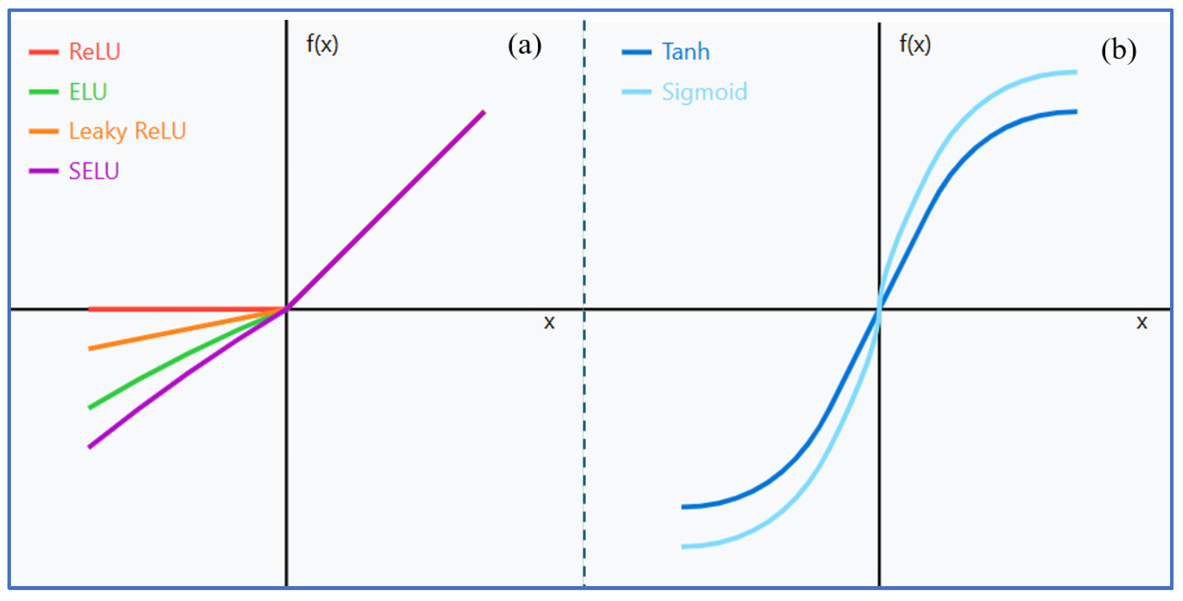
• Activation functions (ReLU, tanh, ELU, SELU, Leaky ReLU, and sigmoid) (Equations (1)–(6)).

Figure 4 illustrates these activation functions, grouped into two families. The ReLU family (Figure 4a) includes the following:

ReLU: f(x) = max(0,x)

(1)

ELU: f(x) = x if x > 0 else α(e^x − 1),

(2)

where α is a positive constant

Leaky ReLU: f(x) = x if x > 0 else αx,

(3)

where α is a small positive constant

SELU: f(x) = λx if x > 0 else λα(e^x − 1),

(4)

where λ and α are learned parameters.

The sigmoid family (Figure 4b) includes the following:

$$\mathrm{Tanh:} \mathrm{f}(\mathrm{x})={\displaystyle \frac{e^x-e^{-x}}{e^x+e^{-x}}}$$

(5)

$$\mathrm{Sigmoid:} \mathrm{f}(\mathrm{x})={\displaystyle \frac{1}{1+e^{-x}}}$$

(6)

This approach differs from our previous study [25] in several ways. In our earlier work, we fixed the number of hidden layers at 4, but allowed each layer to have different numbers of neurons (ranging from 20 to 44 in increments of 2) and different activation functions (choosing from ELU, ReLU, tanh, and sigmoid). This resulted in 13 possible neuron counts and 4 activation functions for each of the 4 layers, leading to (13 × 4)⁴ = 331,776 possible combinations. Given this large search space, we randomly sampled 100 combinations for evaluation.

In contrast, our current approach explores different network depths, while maintaining consistency across layers (same number of neurons and activation function for all hidden layers). We also expanded our activation function options by adding SELU and Leaky ReLU. This new approach results in 4 (layer options) × 4 (neuron options) × 6 (activation functions) = 96 possible combinations, allowing us to exhaustively evaluate all possibilities, rather than relying on random sampling.

We implemented a systematic grid search across these hyperparameters using TensorFlow. The model training utilized the Adam optimizer with the mean squared error (MSE) loss function, chosen for its effectiveness in regression tasks and adaptability to varying gradients. To prevent overfitting and ensure model generalization, we implemented early stopping with validation loss monitoring (patience = 50 epochs). The optimization process involved stratified data splitting (60% training, 20% validation, 20% testing), standardization of numerical features (EC, X2), and one-hot encoding of categorical variables (Location, WYT, Month). The preprocessing pipeline was preserved using joblib to ensure consistent transformation of future data points, which is crucial for model deployment and operational use.

2.2.3. Model Evaluation Metrics

Model evaluation in water quality prediction requires careful consideration of both prediction accuracy and generalization capability. We established an evaluation framework incorporating multiple complementary metrics and validation strategies to ensure robust assessment of model performance.

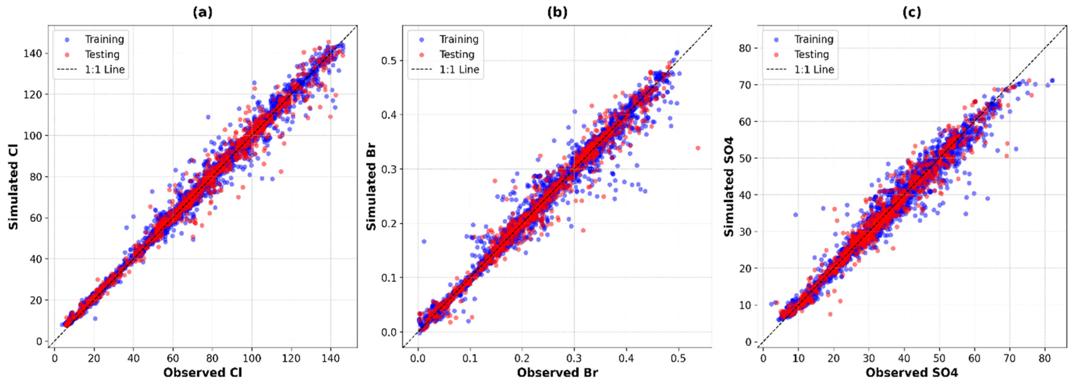
Our evaluation framework centered on three primary performance metrics, each capturing different aspects of model performance. The coefficient of determination (R²), defined in Equation (7), quantifies the proportion of variance in the observed data explained by the model. While higher values indicate a better model fit, R² alone can be misleading, as it is sensitive to the range and distribution of the data. However, its widespread use in water quality modeling studies makes it valuable for comparing results across different research efforts and methodologies. The Mean Absolute Error (MAE, Equation (8)) provides a direct measure of prediction accuracy in the original units of measurement (mg/L), making it particularly valuable for operational applications. Unlike R², the MAE is less sensitive to outliers and offers more interpretable results. The magnitude of acceptable MAE varies by constituent, considering its typical concentration range and operational requirements. The third metric, Percentage Bias (PBIAS, Equation (9)), reveals systematic over- or under-prediction tendencies in the model. Positive values indicate overestimation, while negative values suggest underestimation. In water quality applications, consistent bias could significantly impact treatment processes and management decisions, making PBIAS an essential metric for operational reliability assessment.

We implemented a multi-layered validation approach to ensure robust evaluation of model performance. The dataset was divided into three subsets through random stratified sampling: 60% for training, 20% for validation during model development, and 20% reserved as an independent test set. This split ensured unbiased evaluation of final model performance on previously unseen data, while maintaining similar statistical distributions across all sets. The comparison of performance metrics between training and test sets served as a crucial check for potential overfitting, where small differences indicate good generalization, while large discrepancies would suggest model reliability issues requiring refinement.

The performance metrics are defined as follows:

$$R^2=1-{\displaystyle \frac{\sum {(y_{true}-y_{pred})}^2}{\sum {(y_{true}-\overline{y})}^2}}$$

(7)

$$MAE={\displaystyle \frac{\sum \left|y_{pred}-y_{true}\right|}{n}}$$

(8)

$$\mathrm{P}\mathrm{B}\mathrm{I}\mathrm{A}\mathrm{S}=100\times {\displaystyle \frac{\sum (y_{pred}-y_{true})}{\sum \left(y_{true}\right)}}$$

(9)

where $y_{true}$ represents observed values, $y_{pred}$ represents predicted values, ȳ is the mean of observed values, and $n$ is the number of observations.

To further assess model stability and generalization capabilities, we implemented a k-fold cross-validation analysis (k = 5). This approach systematically partitions the data into five equal folds, using four folds for training and one for testing, rotating through all possible combinations. We maintained consistent preprocessing across all folds using Scikit-learn’s ColumnTransformer, which included standardization of numerical features (EC, X2) and one-hot encoding of categorical variables (Location, WYT, Month). For each fold, we loaded the previously trained models and preprocessors for each ion constituent, then evaluated their performance using the three metrics mentioned above (R², MAE, and PBIAS). This cross-validation implementation was performed independently for each ion constituent (chloride, bromide, and sulfate), allowing us to assess the stability of model performance across different subsets of data and different constituents. The analysis was automated using the TensorFlow and Scikit-learn libraries, ensuring consistent evaluation procedures across all folds and constituents. This systematic approach provides a more reliable estimate of model performance than single train-test splits, which was particularly important given the temporal and spatial variability in our water quality data.

2.3. Dashboard Development

Web-based dashboards offer significant advantages for water quality management tools, providing universal accessibility, real-time updates, and interactive visualizations without requiring local software installation. Our implementation leverages Microsoft Azure’s Web Apps service, a cloud computing platform that provides scalable hosting infrastructure [41]. Azure Web Apps manage server maintenance, security updates, and load balancing, allowing the applications to efficiently handle multiple concurrent users. The system’s computational resources are adjustable based on usage demands—if additional processing power is needed to handle more users or complex calculations, the cloud computing capacity can be increased by upgrading the subscription level. During periods of lower demand, capacity can be scaled down to optimize costs.

The development infrastructure uses GitHub (https://github.com/, accessed on 1 June 2022) as a version control and code hosting platform, integrated with Azure through continuous integration and deployment (CI/CD) pipelines. When code updates are pushed to GitHub, Azure automatically deploys these changes to the production environment after running automated tests, ensuring rapid updates while maintaining system stability. The cloud resources are configured based on anticipated computational needs and usage patterns, with subscription levels adjusted monthly to balance performance and cost.

All three dashboards share a common technical foundation, built using Python’s scientific computing stack [42]. The visualization layer employs Panel for creating interactive web interfaces and HoloViews for generating dynamic plots [43]. These libraries were chosen for their ability to create responsive, interactive visualizations, while efficiently handling large datasets [30]. Bokeh serves as the underlying plotting library, enabling the creation of interactive plots that can be updated in real time as users adjust parameters [44]. The dashboards use a consistent set of UI components, such as sliders, dropdown menus, and buttons, to provide a familiar user experience across applications.

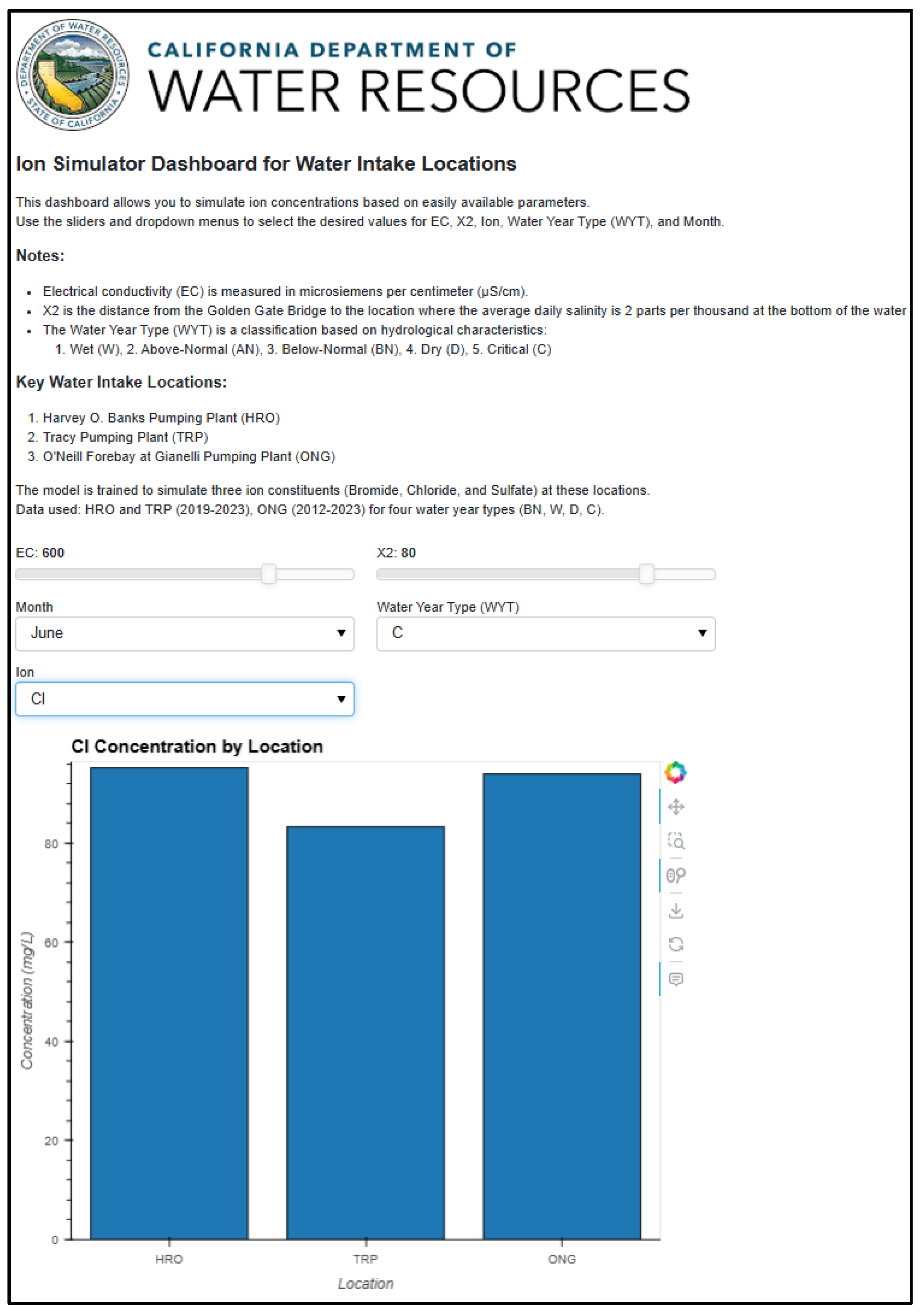
The Water Intake Locations Dashboard focuses on water intake locations, providing real-time predictions of ion concentrations based on user-specified parameters. Users can adjust parameters like EC, Sacramento X2, Water Year Type, and Month, with results displayed through interactive bar charts that compare different model predictions. By relying on pre-trained models, this dashboard delivers fast predictions without requiring the computational overhead of training models on-the-fly.

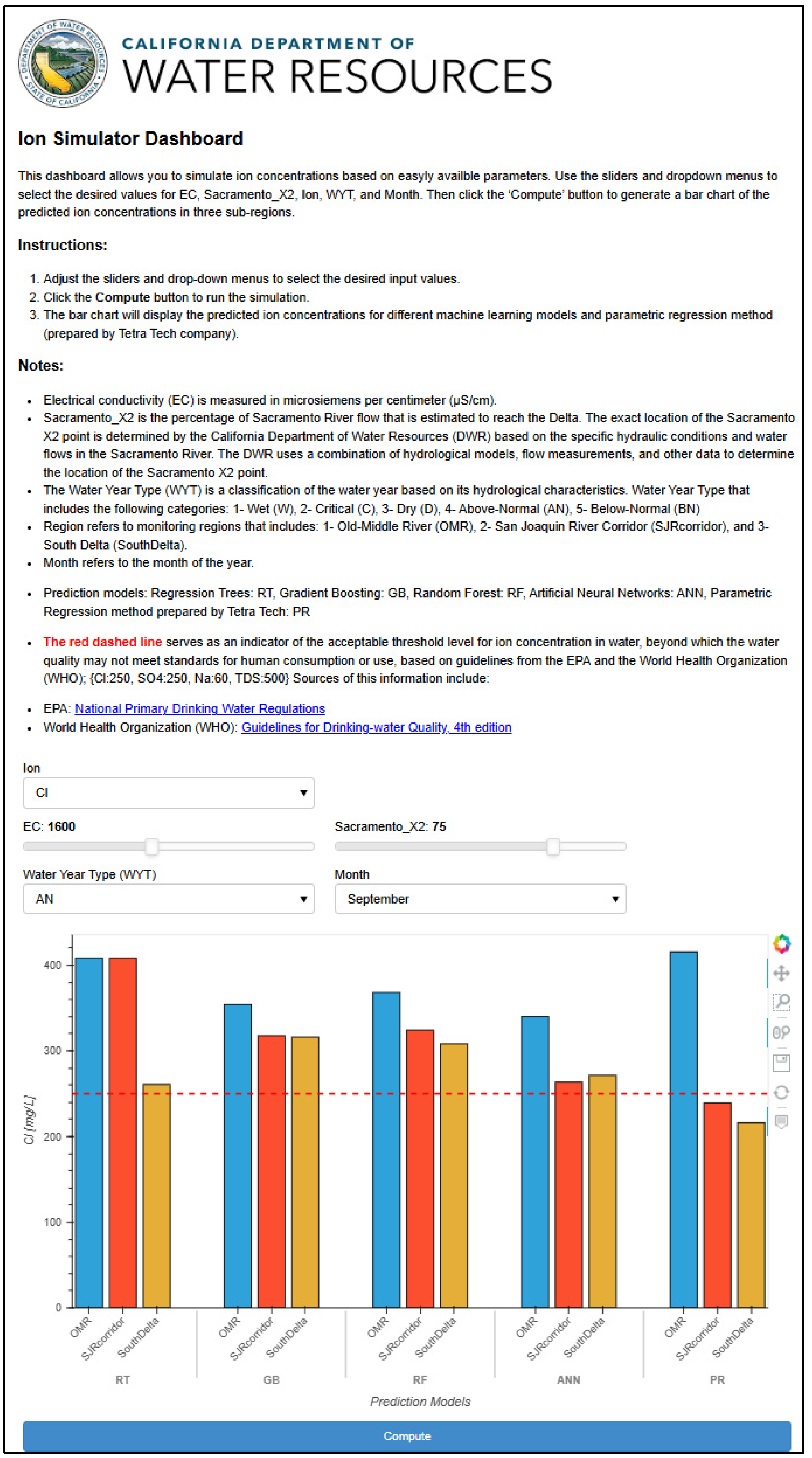
The Enhanced Interior Delta Dashboard extends our previous Interior Delta dashboard [25] by integrating Hutton et al.’s parametric regression equations alongside machine learning predictions [21]. This integration enables direct comparisons between four machine learning approaches—Regression Trees (RTs), Gradient Boosting (GB), Random Forest (RF), and Artificial Neural Networks (ANNs)—and the classical parametric method across three sub-regions. The dashboard also includes horizontal threshold lines for key ion constituents (chloride: 250 mg/L, sulfate: 250 mg/L, sodium: 60 mg/L, and total dissolved solids: 500 mg/L), allowing users to quickly identify when predicted concentrations exceed acceptable water quality standards [45].

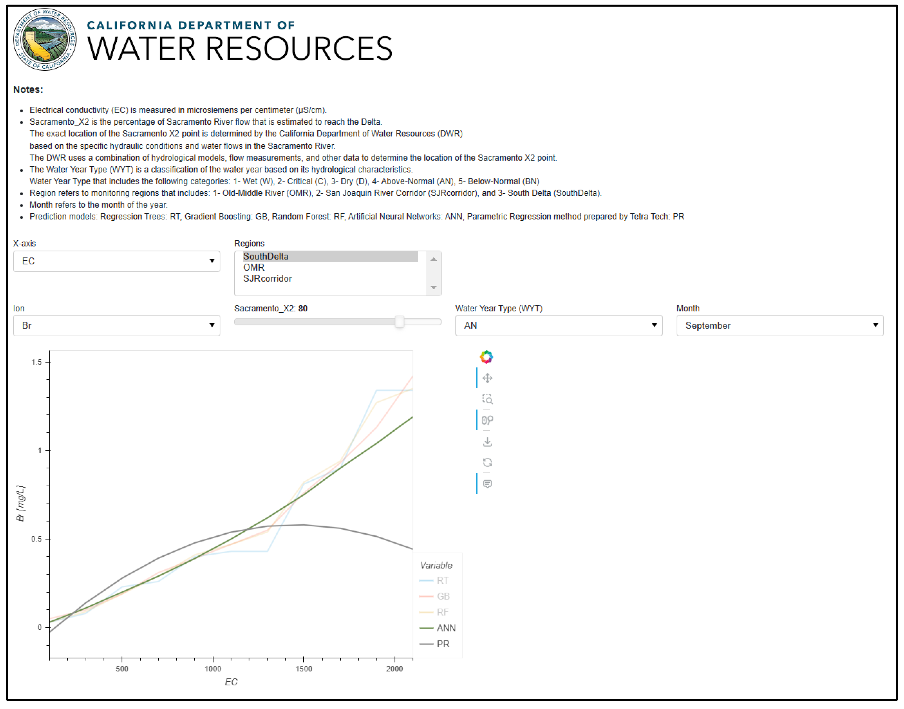
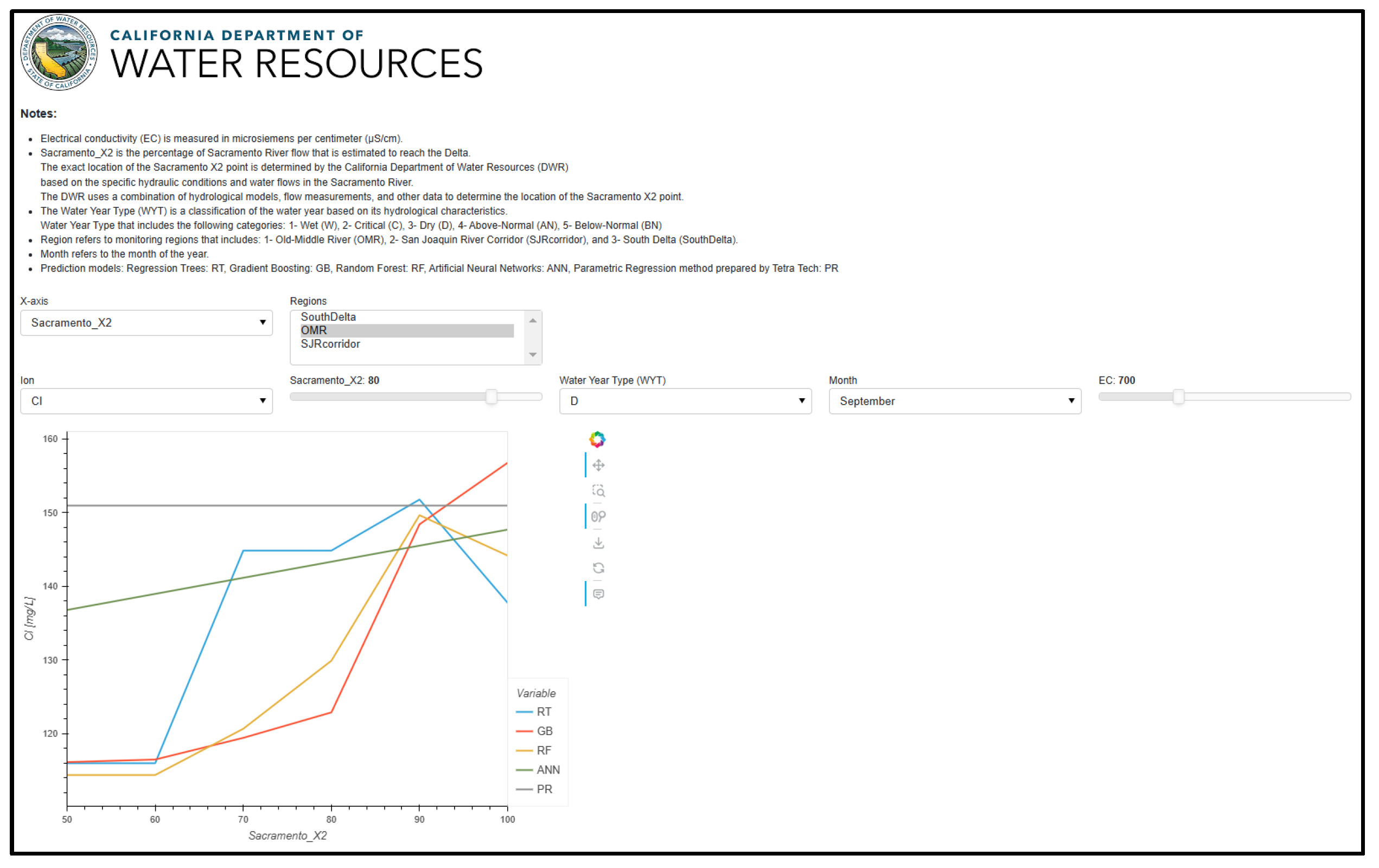
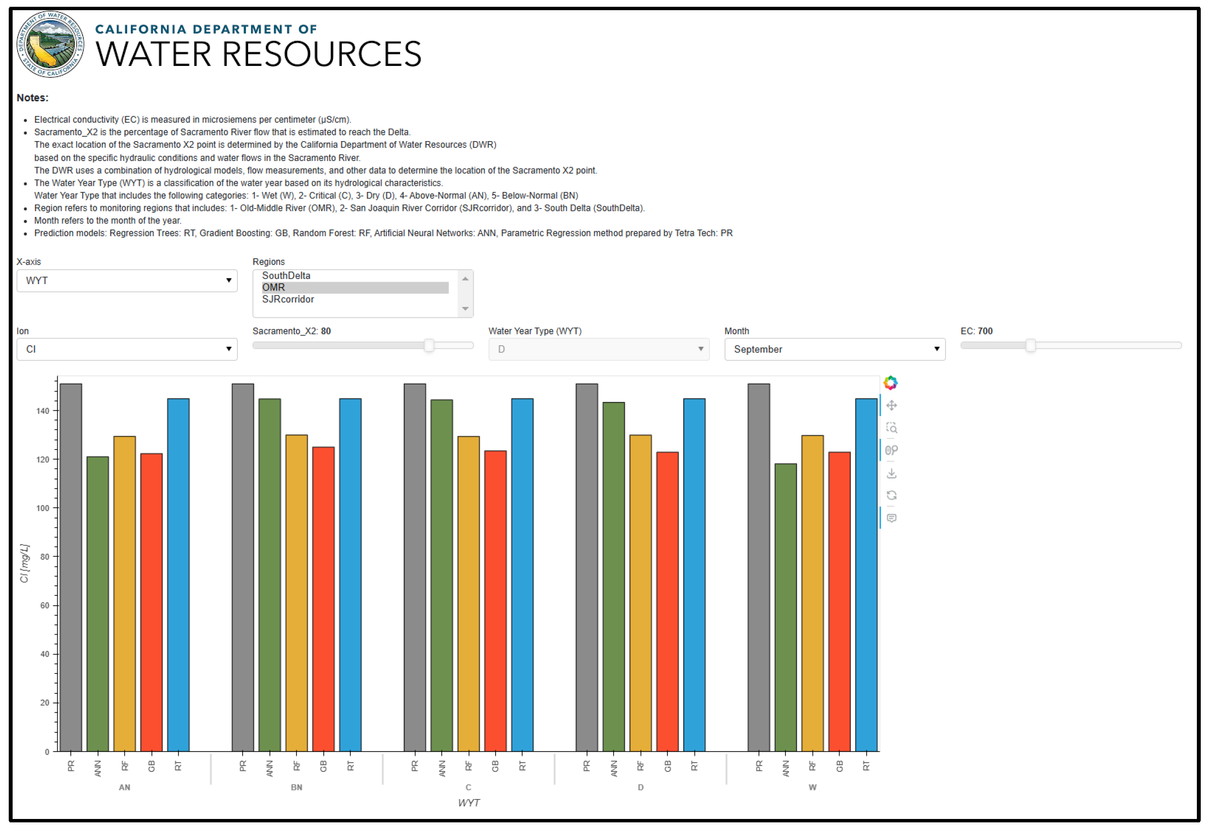
The Model Interpretability Dashboard serves as an analytical tool to help users understand how different parameters influence ion predictions. Users can select any input parameter—such as EC, Sacramento X2, Water Year Type, or Month—as the x-axis to observe changes in ion concentrations across its full range, while keeping other variables constant. This functionality allows users to perform the following:

• Analyze the sensitivity of predictions to different input variables.
• Compare how different regions respond to parameter changes.
• Understand model behavior under various conditions.
• Assess model stability across different parameter ranges.
• Compare predictions from different modeling approaches (ML vs. classical methods).

The dashboard uses a cache-based system to optimize performance. For first-time parameter combinations, comprehensive calculations are performed, which may take a few seconds. However, these results are cached, enabling instant response times for subsequent queries with the same parameters. This caching mechanism is especially valuable for sensitivity analyses, where users often explore similar scenarios. The visualizations include interactive line plots for continuous variables and bar charts for categorical parameters, with options to display multiple regions and prediction methods simultaneously [43].

Each dashboard maintains its own logging system to track usage patterns and performance metrics, which informs future optimizations and resource allocation. Error handling and input validation are implemented to ensure robustness, and responsive design principles are applied to ensure usability across different devices and screen sizes.

2.4. Addressing Model Limitations Through a Hybrid Approach

While both machine learning and classical approaches have demonstrated strong predictive capabilities for ion constituents, they share two fundamental limitations. First, predictions are constrained to specific monitoring locations, lacking continuous spatial coverage across the Delta. Second, neither approach can independently evaluate potential future scenarios, limiting their utility for long-term planning and climate change impact assessment.

To overcome these limitations, we developed a hybrid water quality model that integrates the Delta Simulation Model 2 (DSM2) with our machine learning framework. DSM2 is a well-established hydrodynamic and water quality model used extensively for simulating water conditions in the Delta [45]. DSM2 can simulate EC across an extensive network of nodes throughout the Delta, providing spatial and temporal detail that can be leveraged to enhance prediction capabilities.

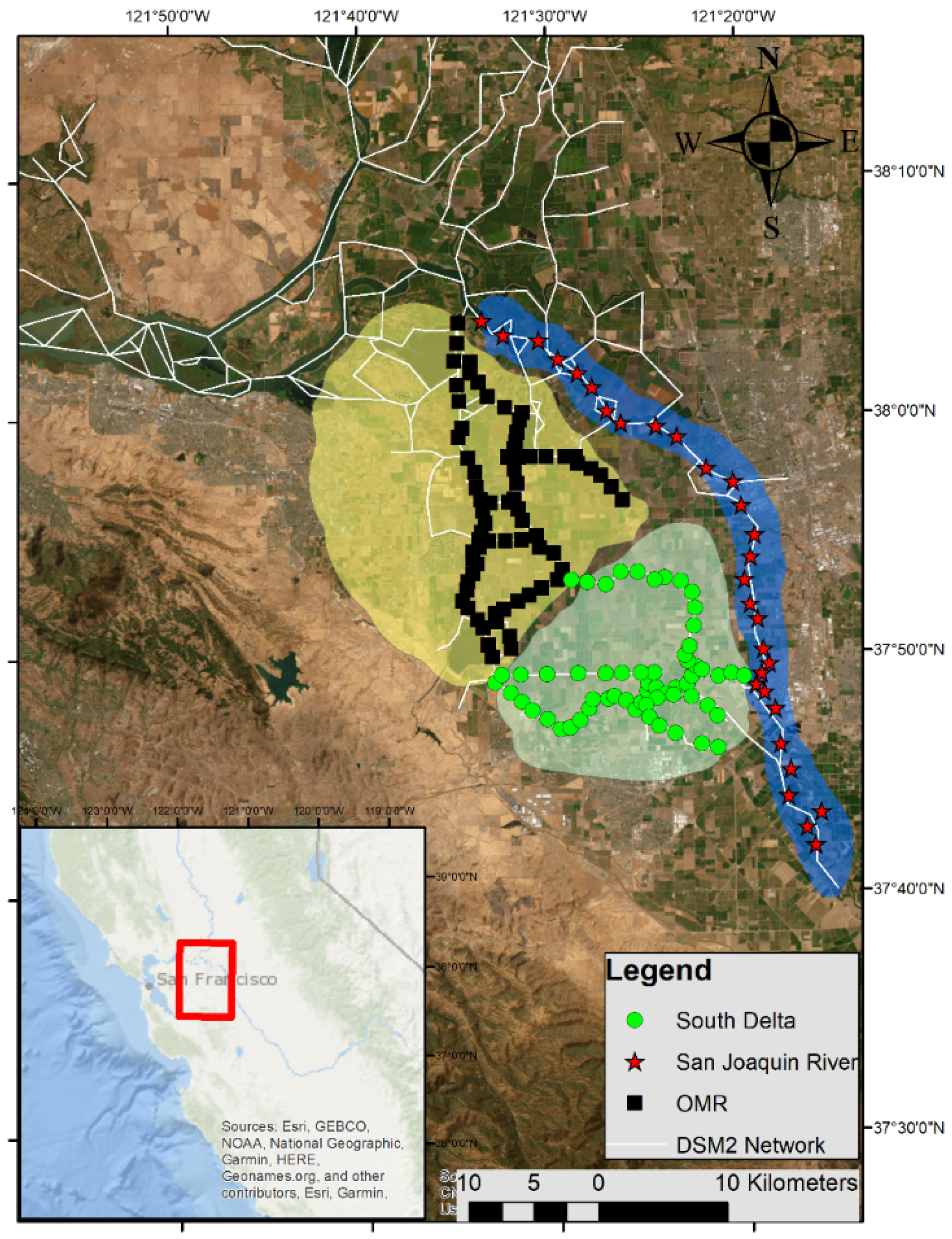
For this hybrid approach, we selected 162 points across three key sub-regions: 60 in the South Delta (yellow circles), 30 along the San Joaquin River corridor (red stars), and 72 in the Old–Middle River corridor (black squares), as illustrated in Figure 5. These points were carefully positioned to capture key water quality gradients and hydrodynamic features across the Delta system while maintaining computational efficiency. This strategic distribution ensures comprehensive coverage of critical areas and enables effective spatial interpolation between monitoring locations. The hybrid model operates in two stages:

• DSM2 simulation: DSM2 is used to generate EC values at all 162 points, ensuring extensive spatial and temporal coverage.
• ANN predictions: the simulated EC values are then used as inputs for our ANN model to predict ion concentrations at these points.

This hybrid model offers several advantages:

• Continuous spatial coverage: the use of DSM2 provides simulated EC values across much of the Delta’s channel network, enabling spatial interpolation between the selected points to create a more continuous ion concentration map.
• Temporal flexibility: DSM2 can generate EC data for any desired time period, from historical conditions to future projections (for example in this project: 2000–2023), providing complete temporal coverage.
• Scenario analysis: the model’s capability to modify DSM2 input parameters allows for evaluation of future scenarios, such as changes in climate, hydrology, or operational practices.
• Combining physics-based and data-driven insights: by integrating DSM2, a process-based model, with the ANN, a data-driven model, the hybrid system benefits from both detailed physical simulation and the flexibility of machine learning.

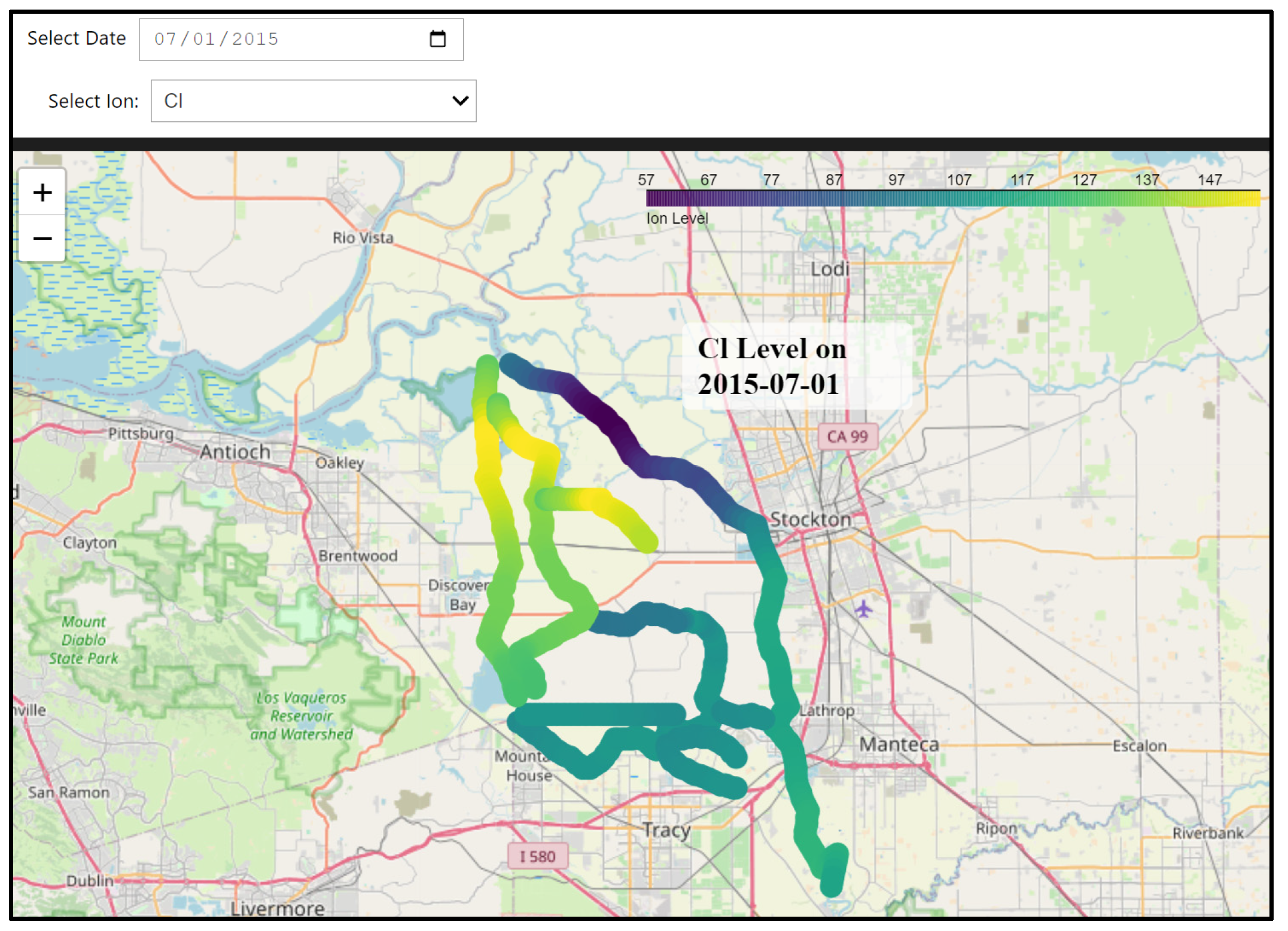
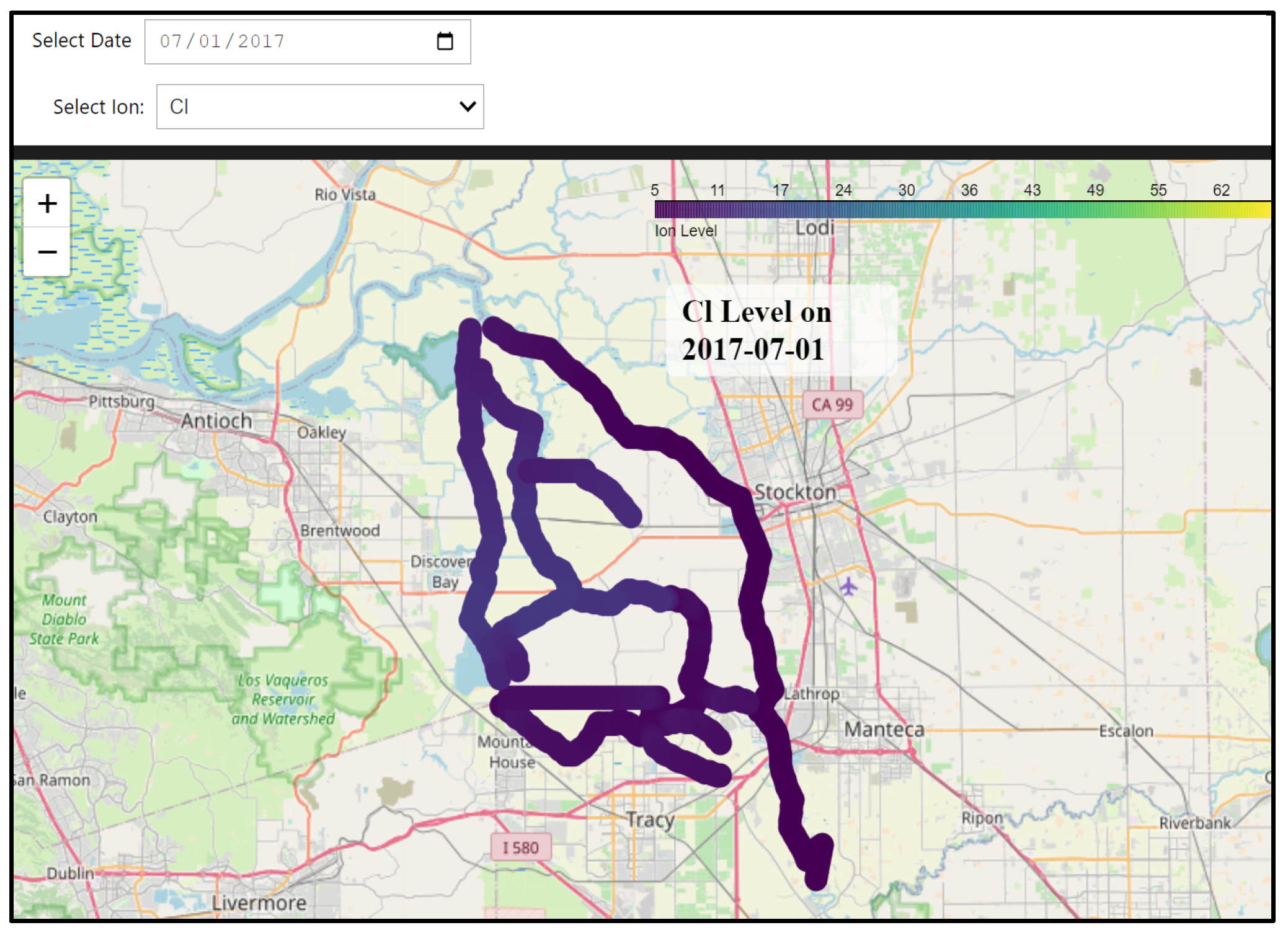
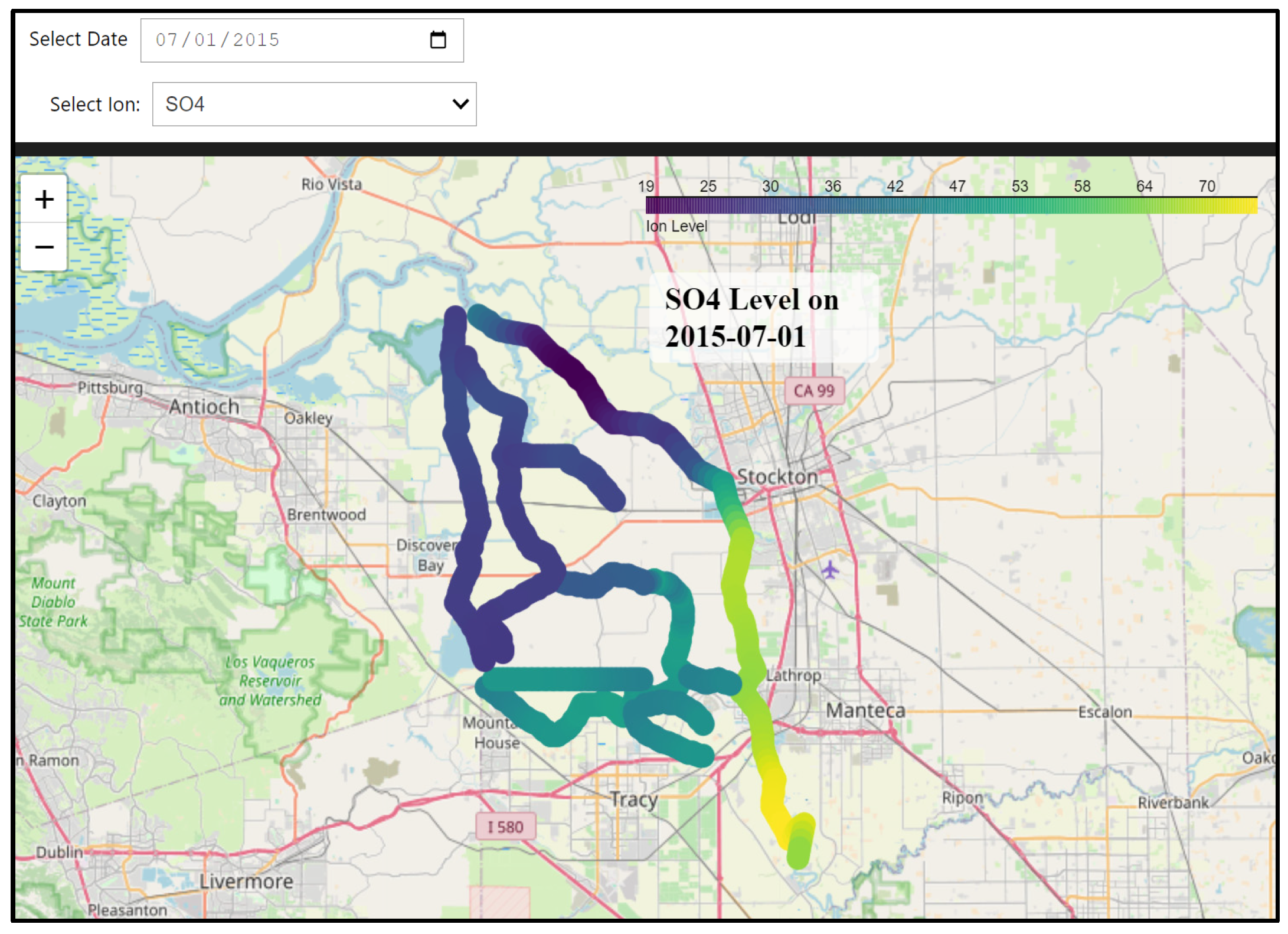
To make this hybrid model accessible, we developed a dedicated dashboard that visualizes spatial distributions of ion concentrations throughout the Delta. Users can select specific dates and ion constituents to view the spatial patterns on an interactive map. Due to the computational intensity of these calculations, particularly involving spatial interpolation, this dashboard is designed for local deployment, rather than cloud hosting. The full codebase is available through our GitHub repository, allowing users to conduct their analyses on local machines with their own computational resources.

This hybrid approach bridges the gap between localized predictions and broader spatial–temporal analysis, enabling scenario planning and improving water quality management throughout the Delta. The ability to produce continuous spatial distributions of ion concentrations represents a significant step forward in our capacity to understand and manage the complex dynamics of the Delta ecosystem.

3. Results

3.1. Model Performance at Water Intake Locations

The performance evaluation of our models began with identifying optimal hyperparameters for each constituent.

Table 2. Optimal neural network architectures for each constituent.

Constituent	Number of Layers	Neurons per Layer	Activation Function
Chloride	3	40	tanh
Bromide	4	40	relu
Sulfate	5	40	tanh

presents the optimal network architectures derived from our hyperparameter optimization process.

While all constituents achieved optimal performance with 40 neurons per layer, they required different network depths and activation functions. Chloride predictions were optimized with a relatively simple architecture (three layers), while sulfate required a deeper network (five layers), suggesting varying levels of complexity in the underlying relationships between input features and constituent concentrations.

Table 3. Model performance metrics for water intake locations.

Constituent	Dataset	R2	MAE (mg/L)	Percentage Bias (%)
Chloride	Training	0.988	2.017	−0.02%
	Test	0.981	2.672	−0.39%
Bromide	Training	0.975	0.01	−0.22%
	Test	0.971	0.011	−0.41%
Sulfate	Training	0.969	1.502	−0.24%
	Test	0.962	1.774	−0.01%

presents the detailed performance metrics for these optimized models on both the training and test datasets.

The models demonstrated strong performance across all constituents, with R² values above 0.96 for all test cases. The small differences between the training and test performance metrics (ΔR² ≤ 0.007) indicate good generalization capabilities. The minimal bias in predictions (all < 0.5%) further supports the reliability of these models for operational use. When evaluating the Mean Absolute Error (MAE), it is crucial to consider the distinct concentration ranges for each constituent at the water intake locations, as shown in Figure 2. Chloride concentrations typically range from 20 to 140 mg/L, while bromide varies between 0 and 0.5 mg/L, and sulfate ranges from 20 to 80 mg/L. Given these different scales, the MAE values (chloride: 2.672 mg/L, bromide: 0.011 mg/L, sulfate: 1.774 mg/L) should be evaluated relative to each constituent’s typical concentration range, rather than compared directly across constituents. For example, the chloride model’s MAE of 2.672 mg/L represents approximately 2.2% of its maximum observed concentration range, while the bromide model’s MAE of 0.011 mg/L represents about 2.2% of its range, indicating comparable relative performance, despite very different absolute MAE values. To visualize the prediction accuracy across these different concentration ranges, Figure 6 presents scatter plots of the predicted versus observed values for all three constituents.

The scatter plots reveal several important characteristics of the models’ performance across the three constituents. For Chloride (Figure 6a), the model demonstrates excellent prediction accuracy across the full range of 0–146 mg/L, with particularly tight clustering around the 1:1 line at low-to-medium concentrations. While there is slightly increased scatter at higher concentrations (>100 mg/L), the model maintains overall accuracy. The nearly identical patterns between the training and test points indicate robust generalization capabilities.

Bromide predictions (Figure 6b) show notably high precision in the critical low-concentration range (0–0.2 mg/L) and maintain consistent performance across the entire range of 0–0.5 mg/L. Although some scattered points appear in the mid-range concentrations (0.2–0.3 mg/L), the model effectively maintains the overall trend and captures the relationship well, even in the upper concentration range.

The sulfate model (Figure 6c) exhibits strong performance across the observed range of 0–85 mg/L, with similar prediction patterns between the training and test datasets. Despite slightly increased scatter in the middle range (30–50 mg/L), the model maintains accuracy at both low and high concentration extremes.

Several common features are evident across all three constituents. The even distribution of points around the 1:1 line confirms the low bias shown in Table 3, while the consistent performance between the training and test datasets validates the models’ generalization capabilities. Notably, there are no systematic deviations or patterns that would suggest model limitations, and all models demonstrate robust performance across the full range of environmentally relevant concentrations. These visualizations complement the numerical metrics in Table 3 by demonstrating that the models’ high R² values and low MAEs are achieved consistently across all concentration ranges, not just in specific regions of the prediction space.

To evaluate the effectiveness of our location-specific approach, we conducted a fair comparison using test dataset performance against both the Interior Delta ML model and classical methods. While all three approaches achieved relatively high R² values (water intake location test: 0.962–0.981, Interior Delta test: 0.96–0.97, classical all data: 0.52–0.92), the MAE metric is a more discriminating metric for comparing model performance, particularly given its direct relevance to operational decision-making. Note that for classical methods, results are reported for the entire dataset, as this approach does not employ train–test splitting. Figure 7 presents a heatmap visualization of the percentage improvements in MAE achieved by our water intake locations model’s test performance compared to the Interior Delta test performance and classical method results, ensuring a fair comparison basis across methods.

These results demonstrate that our location-specific optimization approach successfully captures the unique characteristics of water intake locations, leading to more precise predictions across all constituents. The magnitude of these improvements has significant implications for operational decision-making and water quality management at intake facilities.

3.2. Cross-Validation Results and Model Stability

The five-fold cross-validation analysis demonstrated strong and consistent performance across all folds, supporting the robustness of our models.

Table 4. Cross-validation results showing mean ± standard deviation across 5 folds.

Constituent	R2	MAE (mg/L)	PBIAS (%)
Chloride	0.983 ± 0.006	2.345 ± 0.301	−0.083 ± 0.316
Bromide	0.972 ± 0.004	0.011 ± 0.001	−0.324 ± 0.350
Sulfate	0.962 ± 0.001	1.671 ± 0.089	−0.585 ± 0.483

presents the comprehensive cross-validation results, showing the mean and standard deviation of performance metrics for each constituent.

The cross-validation results reveal several important characteristics of model performance across the different constituents. For chloride predictions, the model achieved the highest R² values (0.983 ± 0.006) among all constituents, with the MAE ranging from 2.078 to 2.857 mg/L across folds. The model demonstrated consistent performance, with relatively small variations between folds, and PBIAS values close to zero (−0.083 ± 0.316%) indicate minimal systematic bias in predictions.

Bromide predictions maintained very strong performance, with an R² of 0.972 ± 0.004, and exhibited remarkably consistent MAE (0.011 ± 0.001 mg/L). While showing slightly higher relative bias (−0.324 ± 0.350%) compared to chloride, the bromide model maintained robust predictive capabilities across all folds. Sulfate predictions demonstrated strong and stable performance, with an R² of 0.962 ± 0.001; notably, they had the most consistent R² values, with the lowest standard deviation (±0.001). The MAE values showed good stability at 1.671 ± 0.089 mg/L, though the model exhibited slightly higher negative bias (−0.585 ± 0.483%) compared to other constituents.

The remarkably low standard deviations across all metrics, particularly for R² values (≤0.006), demonstrate the models’ robust generalization capabilities and stability across different data partitions. This consistent performance across folds suggests that the models successfully captured the underlying relationships between input features and ion concentrations, while avoiding overfitting to specific data subsets.

3.3. Dashboard Applications and Enhancements

3.3.1. Water Intake Locations Dashboard

The Water Intake Locations Dashboard employs ANN models to simulate ion constituents (chloride, bromide, sulfate) at three critical water intake locations. The interface features four predictors: EC (0–800 μS/cm), Sacramento X2 (40–90 km), Water Year Type, and Month. Due to the limited data availability period (2019–2023), the models for Harvey O. Banks (HRO) and the Tracy Pumping Plant (TRP) currently cover only three Water Year Types (D, W, and C), while the O’Neill Forebay (ONG), with its longer record (2012–2023), includes BN as well. The Above-Normal (AN) Water Year Type is excluded for all locations; users are advised to use Wet (W) as an approximation for AN conditions. The accuracy of predictions for HRO and TRP is expected to improve as future data collection encompasses more hydrological conditions.

Figure 8 demonstrates the dashboard’s interface design and functionality using a specific example scenario where we simulate chloride concentrations under the following conditions: EC: 600 μS/cm, Sacramento X2: 80 km, Month: June, Water Year Type (WYT): Critical, ion constituent: chloride. In this particular example, when simulating chloride concentrations under the specified conditions, we observe distinct spatial variations: the O’Neill Forebay (ONG) and Harvey O. Banks (HRO) show similar predicted concentrations at around 90 mg/L, while the Tracy Pumping Plant (TRP) exhibits a lower predicted concentration of approximately 83 mg/L. These spatial differences in chloride concentrations under identical input conditions demonstrate how the complex hydrodynamics of the Delta system influence water quality patterns at different intake locations. Users can explore other scenarios by adjusting any of the input parameters, allowing them to investigate how ion concentrations vary under different operational and environmental conditions.

The dashboard’s real-time visualization capabilities enable operators to compare constituent levels across locations simultaneously, evaluate the impacts of changing operational conditions, identify potential water quality concerns, and support rapid operational decision-making through scenario testing. The interface provides essential contextual information about measurement units, parameter definitions, and data coverage periods, ensuring proper interpretation of results. The visualization includes interactive tools for zooming, panning, and data export, represented by the icons on the right side of the plot.

3.3.2. Enhanced Interior Delta Dashboard

Building upon our previous work [25], the dashboard developed in that study has been significantly enhanced to provide comprehensive visualization and comparison capabilities for ion constituent predictions across the Delta. Key enhancements include the following:

Classical Method Integration: The most significant enhancement is the integration of the classical parametric regression method (PR), developed by [21], alongside machine learning predictions (RT, GB, RF, and ANN). This integration offers several benefits:

• Direct visual comparison between classical and ML approaches;
• Simplified access to ion constituent predictions without requiring manual coefficient calculations;
• Enhanced transparency in model comparison for stakeholders;
• Validation of ML predictions against established methodologies.

This unified platform allows water managers to make informed decisions by comparing multiple prediction methods simultaneously, while maintaining the user-friendly interface that characterized our original dashboard. The addition of the PR method particularly addresses stakeholder needs for comparative analysis between traditional and modern prediction approaches.

Spatial Comparison Capability: The dashboard now enables simultaneous visualization of predictions across all three sub-regions (OMR, SJR corridor, and South Delta), revealing important spatial patterns in ion constituent distributions. For instance, under identical predictor conditions (EC, X2, WYT, and Month), the ANN model demonstrates consistently higher chloride concentrations in the OMR region compared to other areas, reflecting its proximity to ocean influences—a primary source of chloride in the system.

Water Quality Standards Integration: A crucial addition is the incorporation of regulatory threshold indicators (shown as red dashed lines) for key constituents, based on guidelines from the United States Environmental Protection Agency (EPA) and the World Health Organization (WHO): chloride: 250 mg/L, sulfate: 250 mg/L, sodium: 60 mg/L, and total dissolved solids: 500 mg/L. These visual threshold indicators enable immediate assessment of water quality compliance across different regions and conditions.

Figure 9 demonstrates the dashboard’s key capabilities through a typical usage case. In this example, chloride predictions are shown for specified conditions (EC: 1600 μS/cm, Sacramento X2: 75 km, Water Year Type: Above-Normal, Month: September) across all three sub-regions. The visualization clearly shows the spatial variation in chloride concentrations, with consistently higher levels in the OMR region across all models. This pattern aligns with the physical geography of the Delta, as the OMR region is situated closer to the San Francisco Bay and the Pacific Ocean, which serve as the primary sources of chloride through seawater intrusion. The other regions, being further inland, typically experience lower chloride concentrations, due to their greater distance from marine influences. The integrated EPA/WHO threshold line (250 mg/L) provides immediate context for water quality compliance assessment, while the side-by-side comparison of different models (RT, GB, RF, ANN, and PR) enables stakeholders to evaluate prediction consistency and model agreement.

3.3.3. Model Interpretability Dashboard

The Model Interpretability Dashboard was developed to provide deeper insights into model behavior and sensitivity for our Interior Delta predictions, focusing on comparing the machine learning models and the classical method presented in our previous study [21]. While our ion constituent simulator dashboard focuses on operational predictions across all locations, this interpretability dashboard specifically examines how different modeling approaches for the Interior Delta respond to variations in input parameters. The dashboard enables analysis of all nine ion constituents against any selected predictor variable, while holding other conditions constant, making it a powerful tool for understanding model dynamics and validating their physical consistency.

Figure 10 demonstrates the dashboard’s capability to analyze model behavior across the EC range for bromide predictions under specific conditions (Sacramento X2 = 80 km, Water Year Type = Above-Normal, Month = September, South Delta region). The visualization reveals distinct behavioral patterns among different models, with the ANN model exhibiting notably smoother response curves compared to other ML approaches. A critical transition point occurs at EC ≈ 1200 μS/cm, where the relative predictions between ANN and the classical method (PR) reverse their relationship. Below this threshold, ANN predicts higher bromide concentrations, while above it, the classical method shows higher predictions. This smooth transition in the ANN model, compared to the more erratic behavior of other ML models, represents an additional advantage beyond its superior statistical performance metrics.

The dashboard’s ability to analyze sensitivity to different predictors is further illustrated in Figure 11, which shows model responses to Sacramento X2 variations for chloride predictions (EC = 700 μS/cm, Month = September, Water Year Type = Dry, OMR region). This comparison reveals significant differences in how models incorporate the X2 influence. The classical method shows no sensitivity to X2 changes under these conditions, producing a flat response that suggests a potential limitation in capturing this important physical relationship. In contrast, the ANN model demonstrates smooth, physically plausible responses to X2 variations. Other ML models (RT, GB, and RF) exhibit high sensitivity to X2 changes with discontinuous jumps in predictions, suggesting potential overfitting to training data points.

The dashboard’s capability to analyze categorical predictors is demonstrated in Figure 12, which examines model behavior across different Water Year Types for chloride predictions under consistent conditions (EC = 700 μS/cm, Sacramento X2 = 80 km, Month = September, OMR region). The classical method (PR) shows limited sensitivity to water year classification, consistently predicting the highest chloride concentrations (approximately 150 mg/L) across all WYTs. The ANN model demonstrates more nuanced and physically plausible behavior, showing a gradual decrease in chloride concentrations from Critical to Wet conditions, while maintaining predictions in the 120–140 mg/L range. Other ML models (RT, GB, and RF) show similar overall patterns, but with more variable responses and generally lower chloride concentration predictions compared to PR and ANN.

These visualizations collectively highlight the ANN model’s superior characteristics beyond traditional performance metrics. Its smoother response surfaces across parameter ranges, more physically consistent behavior, balanced sensitivity to input parameters, and robust predictions without artificial discontinuities make it particularly reliable for operational applications. The Model Interpretability Dashboard proves especially valuable for stakeholders seeking to understand model reliability under different conditions, and for researchers validating model behavior against known physical relationships in the Delta system. This enhanced transparency in model behavior helps to build confidence in the predictions and provides crucial insights for water quality management decisions.

3.4. Hybrid Water Quality Dashboard

The Hybrid Water Quality Dashboard represents a novel integration of DSM2 hydrodynamic modeling with our ANN framework to provide comprehensive spatial coverage of ion constituent concentrations across the Interior Delta. This integration addresses a key limitation of standalone ANN models by enabling predictions at locations without monitoring stations. The dashboard’s architecture combines DSM2-simulated EC values at 162 strategic points (60 in the South Delta, 30 along the San Joaquin River corridor, and 72 in the Old–Middle River corridor) with ANN predictions to generate spatially continuous constituent distributions.

Figure 13 demonstrates the dashboard’s visualization capabilities through a bromide concentration map for 1 July 2015. The interface features a date selector and ion constituent dropdown menu, allowing users to explore temporal and chemical variations across the Delta. The example reveals distinct spatial patterns in bromide concentrations, with values ranging from 0.17 to 0.51 mg/L. A clear gradient is visible from the northern Delta (higher concentrations shown in purple/blue) to the southern regions (lower concentrations in green/yellow), reflecting the complex interplay of tidal influences and river inflows.

Figure 13 and Figure 14 demonstrate temporal variations in chloride concentrations by comparing Critical (2015) versus Wet (2017) water year conditions for July 1st. In the critical year (Figure 13), higher chloride concentrations are evident throughout the Delta, particularly in the OMR corridor, reflecting increased seawater intrusion due to reduced Delta outflow. In contrast, the Wet year (2017, Figure 14) shows notably lower chloride concentrations across all regions, as higher precipitation and river inflows create stronger seaward gradients that limit ocean-derived chloride intrusion.

Figure 15 illustrates spatial patterns of sulfate concentrations during the same period as Figure 13 (1 July 2015). The distribution reveals the highest sulfate levels along the San Joaquin River corridor and South Delta region, with concentrations decreasing notably in the OMR area. This pattern reflects the primary source of sulfate in the Delta system—agricultural drainage inputs predominant in the San Joaquin River and South Delta regions. The distinct spatial patterns between chloride (Figure 13) and sulfate (Figure 15) demonstrate how different sources—seawater intrusion versus agricultural drainage—create unique constituent distributions across the Delta.

The dashboard employs an intuitive color-coding scheme for concentration visualization, with a continuous scale that enables easy identification of spatial gradients and potential water quality concerns. Users can zoom and pan across the Delta region to examine specific areas of interest, while the base map provides geographical context through landmarks and waterway configurations. Unlike our Azure-hosted dashboards, this tool is available through GitHub for local deployment, allowing users to conduct intensive spatial analyses with their own computational resources.

This hybrid approach extends the temporal coverage from 2000 to 2023, providing historical context for water quality patterns. The combination of DSM2’s hydrodynamic simulation capabilities with ANN’s constituent prediction accuracy creates a powerful tool for understanding large-scale water quality dynamics in the Delta system. The spatial interpolation between the 162 monitoring points enables visualization of continuous concentration gradients, offering insights into water quality transitions that would be difficult to discern from point measurements alone.

For enhanced accessibility, we developed three Azure-hosted dashboards and one GitHub-hosted solution, as summarized in

Table 5. Summary of developed dashboards with web links.

Dashboards	Dashboard ID	Web Links
Interior Delta Dashboard	DD1	https://dwrdashion.azurewebsites.net/Dashboard (accessed on 1 March 2025)
Interpretability Dashboard	DD2	https://dwrdashionsensitivity.azurewebsites.net/Sensitivity_IonStudy (accessed on 1 March 2025)
Water Intake Locations Dashboard	DD3	https://dwrdashionintake.azurewebsites.net/Intake_dashboard (accessed on 1 March 2025)
Hybrid Water Quality Dashboard	DD4	https://github.com/PeymanHNamadi/Hybrid_WaterQualityDashboard (accessed on 1 March 2025)

. The Azure-hosted dashboards (Interior Delta, Interpretability, and Water Intake Locations) are optimized for both desktop and mobile access, with QR codes provided for convenient mobile deployment. These QR codes enable stakeholders to quickly access the dashboards from their smartphones or tablets, facilitating real-time decision-making in the field. The mobile interface maintains all the functionality of the desktop version, while adapting to smaller screens.

4. Discussion

The development and implementation of machine learning approaches for ion constituent prediction in the Sacramento–San Joaquin Delta represents a significant advancement in water quality monitoring and management. Our results demonstrate both the technical advantages of these new methods and their practical utility for operational decision-making. This discussion examines the implications of our findings across several key dimensions: model performance and reliability, operational utility, and broader implications for water quality management.

4.1. Model Performance and Reliability

The superior performance of our location-specific ANN models compared to both the Interior Delta ML model and classical methods highlights several important considerations in water quality modeling. The substantial improvements in Mean Absolute Error (MAE)—ranging from 24% for TDS to 59% for sulfate—demonstrate that tailoring models to specific monitoring locations can significantly enhance prediction accuracy. This improvement likely stems from the models’ ability to capture location-specific relationships between Electrical Conductivity and ion constituents, which vary considerably across the Delta system.

The cross-validation results, showing remarkably low standard deviations across all metrics (e.g., R² variations ≤ 0.006), confirm the robust generalization capabilities of our models. This stability is particularly noteworthy given the complex and dynamic nature of the Delta system, where multiple factors influence water quality simultaneously. The consistent performance across different data partitions suggests that the models have successfully captured underlying physical relationships, rather than simply fitting to training data patterns.

However, it is important to acknowledge certain limitations in our approach. The relatively short data record for some locations (2019–2023 for HRO and TRP) means that the models have not been exposed to the full range of possible hydrological conditions. While performance metrics remain strong, continued validation against new data will be crucial for ensuring long-term reliability. Additionally, the current exclusion of Above-Normal Water Year Types from some location-specific models represents a gap that should be addressed as more data become available.

4.2. Operational Utility and Dashboard Implementation

The Water Intake Locations Dashboard’s (DD3) focus on critical infrastructure points demonstrates how location-specific optimization can enhance operational relevance. The real-time visualization capabilities and mobile accessibility through QR codes reflect a practical understanding of how these tools will be used in the field. However, the dashboard’s current limitations regarding Water Year Types highlight the ongoing need for data collection and model refinement.

The development of three complementary dashboards, each serving different user needs, represents a significant step forward in making complex modeling tools accessible to water managers. The Enhanced Interior Delta Dashboard’s (DD1) integration of classical methods alongside machine learning predictions provides a valuable bridge between traditional and modern approaches, helping to build user confidence through direct comparison. The addition of regulatory threshold indicators directly addresses operational needs by providing immediate visual feedback on water quality compliance.

The Model Interpretability Dashboard addresses (DD2) a crucial challenge in the adoption of machine learning methods: the perceived “black box” nature of these models. By enabling users to visualize how models respond to different predictors and operating conditions, this tool helps to build trust in ML predictions. The smooth response curves demonstrated by the ANN model, particularly in comparison to other ML approaches, suggest that it has captured physically meaningful relationships, rather than arbitrary patterns in the training data.

Our hybrid approach, combining DSM2 hydrodynamic modeling with ANN predictions, represents a significant advancement in addressing spatial coverage limitations inherent in point-based monitoring systems. The ability to generate continuous spatial distributions of ion concentrations provides water managers with unprecedented insight into water quality dynamics across the Delta. This capability is particularly valuable for understanding how different operational decisions might affect water quality throughout the system, not just at monitoring locations.

The dashboard implementation strategy, using both cloud-hosted and locally deployed solutions, balances accessibility with computational requirements. The Azure-hosted dashboards provide widespread access to essential prediction tools, while the GitHub-hosted hybrid model enables more intensive analyses when needed. This dual approach ensures that different stakeholder needs can be met effectively, while managing computational resources efficiently.

5. Conclusions

This research introduces new machine learning tools for simulating ion constituents in California’s Sacramento–San Joaquin Delta. Our approach advances water quality monitoring through improved prediction accuracy and accessibility. Our work makes three significant contributions:

First, we demonstrated that location-specific ANN models substantially improve prediction accuracy for ion constituents at critical water intake locations (cross-validated R² > 0.96, σ ≤ 0.006).

Second, we developed four complementary web-based tools that make these modeling capabilities accessible to water managers: (1) an Enhanced Interior Delta Dashboard integrating classical and machine learning approaches; (2) a Model Interpretability Dashboard visualizing model behavior; (3) a Water Intake Locations Dashboard providing targeted predictions; and (4) a Hybrid Water Quality Dashboard enabling spatial coverage.

Third, our hybrid modeling approach combines DSM2 hydrodynamic simulations with ANN predictions, enabling continuous spatial prediction of ion constituents across the Delta and addressing the fundamental limitations of point-based monitoring.

Future Research

Our current models effectively simulate present conditions (nowcasting), but future work will focus on forecasting capabilities. We plan to extend these models to predict ion constituent levels 1–7 days in advance, developing an early warning system for water managers. Additionally, we aim to incorporate climate change scenarios into our hybrid model to assess long-term impacts on Delta water quality. As computational capabilities and data collection improve, we envision expanding this approach to model additional water quality parameters and implementing real-time monitoring integration for more responsive management systems.