

The Impact of Inundation and Nitrogen on Common Saltmarsh Species Using Marsh Organ Experiments in Mississippi


Abstract
1. Introduction
2. Materials and Methods
2.1. Study Species
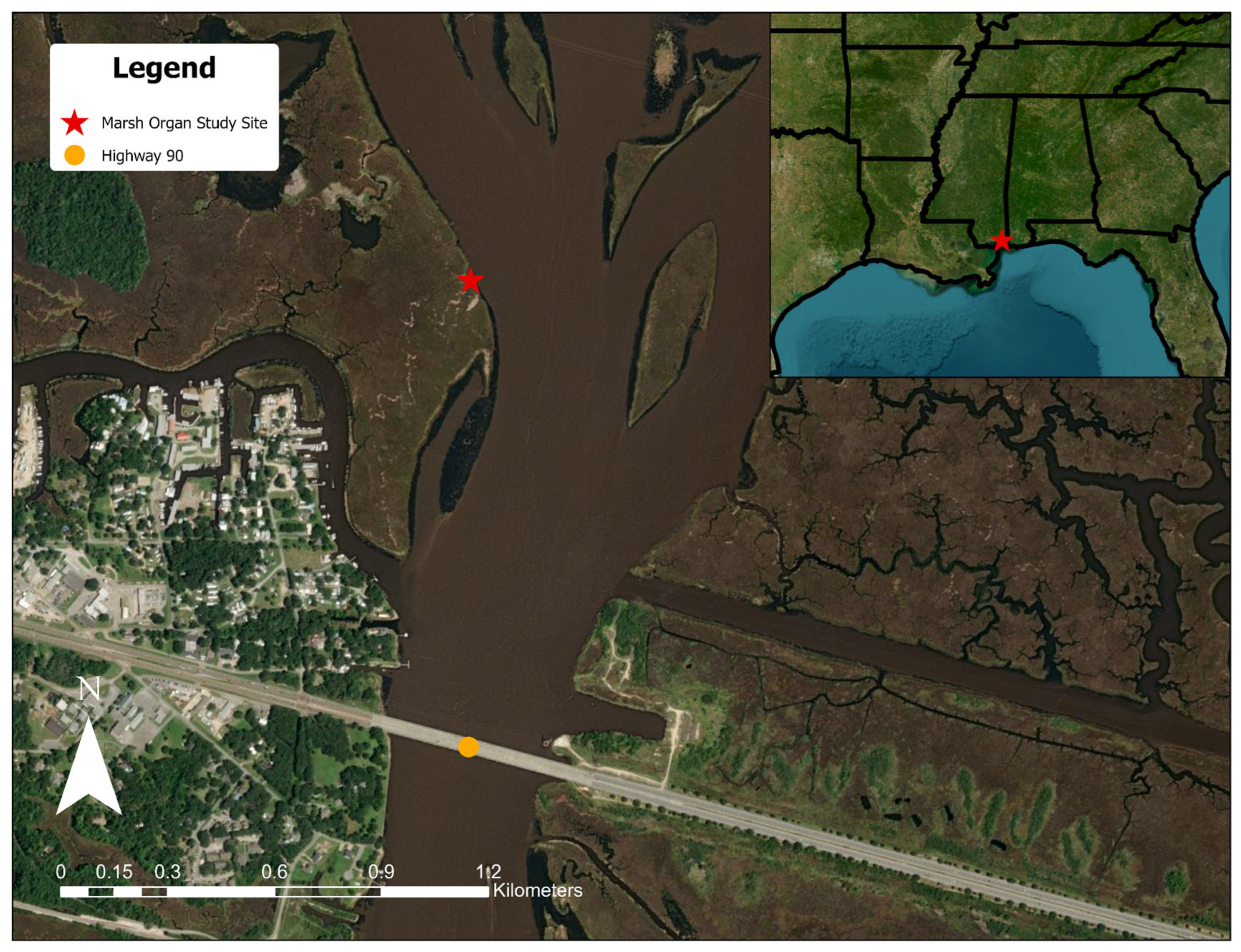
2.2. Study Site
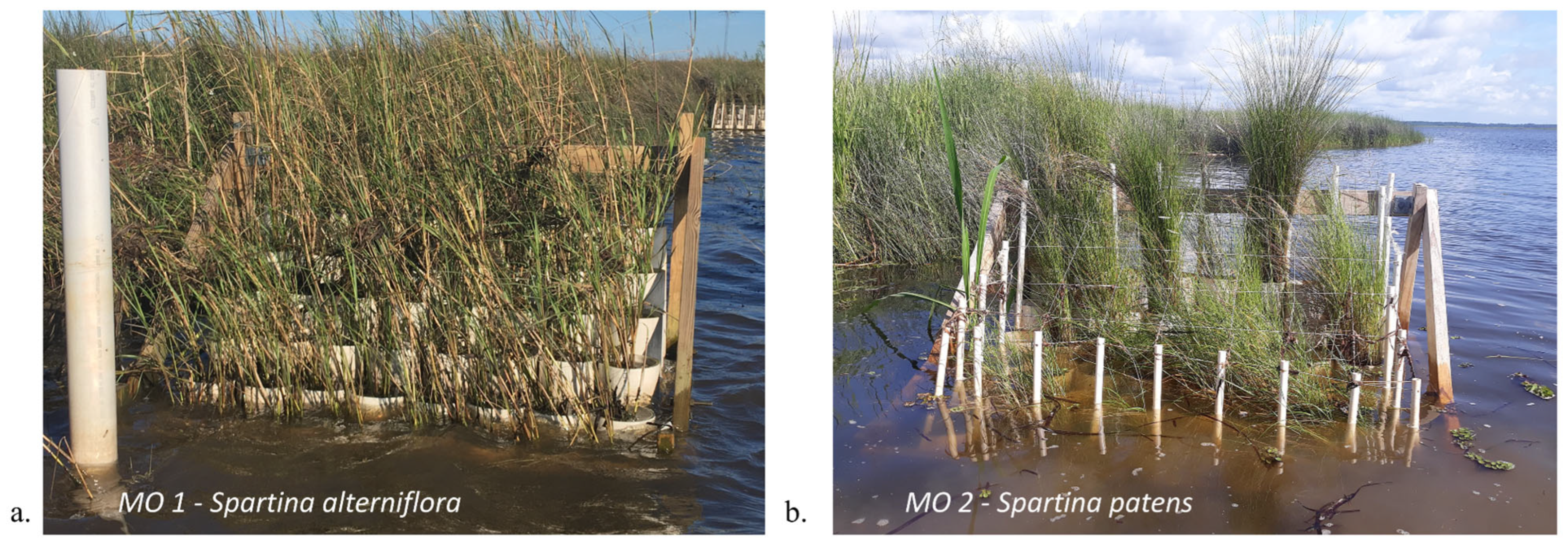
2.3. Marsh Organ Design
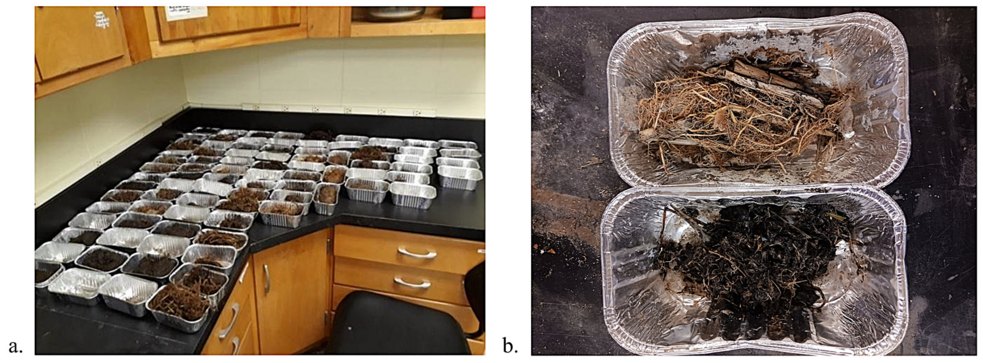
2.4. Trait Monitoring and Biomass Processing
2.5. Statistical Analyses
3. Results
3.1. Inundation Duration
3.2. Response of Aboveground Biomass
3.3. Response of Belowground Biomass
3.4. The Impact of Inundation on Morphological Traits
3.5. The Impact of Nutrients on Morphological Traits
3.6. The Impact of Pre-Condition on Morphological Traits
3.7. The Impact of Senescence or Seasonality on Morphological Traits
3.8. The Impact of Channel on Morphological Traits
4. Discussion
5. Conclusions
Supplementary Materials
Author Contributions
Funding
Data Availability Statement
Acknowledgments
Conflicts of Interest
Abbreviations
| Sa. | Spartina alterniflora |
| Sp. | Spartina patens |
Appendix A


References
- Wu, W.; Biber, P.; Mishra, D.R.; Ghosh, S. Sea-level rise thresholds for stability of salt marshes in a riverine versus a marine dominated estuary. Sci. Total Environ. 2020, 718, 137181. [Google Scholar] [CrossRef] [PubMed]
- Costanza, R.; d’Arge, R.; De Groot, R.; Farber, S.; Grasso, M.; Hannon, B.; Limburg, K.; Naeem, S.; O’neill, R.V.; Paruelo, J.; et al. The value of the world’s ecosystem services and natural capital. Nature 1997, 387, 253–260. [Google Scholar] [CrossRef]
- Engle, V.D. Estimating the provision of ecosystem services by Gulf of Mexico coastal wetlands. Wetlands 2011, 31, 179–193. [Google Scholar] [CrossRef]
- Morris, J.T.; Sundareshwar, P.V.; Nietch, C.T.; Kjerfve, B.; Cahoon, A.D.R. Responses of coastal wetlands to rising sea level. Ecology 2002, 83, 2869–2877. [Google Scholar] [CrossRef]
- Snedden, G.A.; Cretini, K.; Patton, B. Inundation and salinity impacts to above- and belowground productivity in Spartina patens and Spartina alterniflora in the Mississippi River deltaic plain: Implications for using river diversions as restoration tools. Ecol. Eng. 2015, 81, 133–139. [Google Scholar] [CrossRef]
- Langley, A.J.; Mozdzer, T.J.; Shepard, K.A.; Hagerty, S.B.; Patrick Megonigal, J. Tidal marsh plant responses to elevated CO2, nitrogen fertilization, and sea level rise. Glob. Change Bio. 2013, 19, 1495–1503. [Google Scholar] [CrossRef]
- Pellegrini, E.; Incerti, G.; Pedersen, O.; Moro, N.; Foscari, A.; Casolo, V.; Contin, M.; Boscutti, F. Flooding and soil properties control plant intra-and interspecific interactions in salt marshes. Plants 2022, 11, 1940. [Google Scholar] [CrossRef]
- Kirwan, M.L.; Guntenspergen, G.R.; d’Alpaos, A.; Morris, J.T.; Mudd, S.M.; Temmerman, S. Limits on the adaptability of coastal marshes to rising sea level. Geophys. Res. Lett. 2010, 37. [Google Scholar] [CrossRef]
- Pellegrini, E.; Boscutti, F.; De Nobili, M.; Casolo, V. Plant traits shape the effects of tidal flooding on soil and plant communities in saltmarshes. Plant Ecol. 2018, 219, 823–835. [Google Scholar] [CrossRef]
- Kirwan, M.L.; Guntenspergen, G.R. Feedbacks between inundation, root production, and shoot growth in a rapidly submerging brackish marsh. J. Ecol. 2012, 100, 764–770. [Google Scholar] [CrossRef]
- Kirwan, M.L.; Guntenspergen, G.R. Response of plant productivity to experimental flooding in a stable and a submerging marsh. Ecosystems 2015, 18, 903–913. [Google Scholar] [CrossRef]
- McKee, K.L.; Mendelssohn, I.A. Response of a freshwater marsh plant community to increased salinity and increased water level. Aquat. Bot. 1989, 34, 301–316. [Google Scholar] [CrossRef]
- Grimes, E.; Wu, W.; Suir, G. Evaluating the response of Sagittaria lancifolia to combined inundation and nitrogen addition using a marsh organ. Environ. Monit. Assess. 2025, 197, 394. [Google Scholar] [CrossRef] [PubMed]
- Mendelssohn, I.A.; McKee, K.L. Spartina alterniflora die-back in Louisiana: Time-course investigation of soil waterlogging effects. J. Ecol. 1988, 76, 509–521. [Google Scholar] [CrossRef]
- Leonard, L.A.; Croft, A.L. The effect of standing biomass on flow velocity and turbulence in Spartina alterniflora canopies. Estuar. Coast. Shelf Sci. 2006, 69, 325–336. [Google Scholar] [CrossRef]
- Vuerich, M.; Cingano, P.; Trotta, G.; Petrussa, E.; Braidot, E.; Scarpin, D.; Bezzi, A.; Mestroni, M.; Pellegrini, E.; Boscutti, F. New perspective for the upscaling of plant functional response to flooding stress in salt marshes using remote sensing. Sci. Rep. 2024, 14, 5472. [Google Scholar] [CrossRef]
- Nyman, J.A.; DeLaune, R.D.; Roberts, H.H.; Patrick, W.H., Jr. Relationship between vegetation and soil formation in a rapidly submerging coastal marsh. Mar. Ecol. Prog. Series 1993, 96, 269–279. [Google Scholar] [CrossRef]
- Nyman, J.A.; Walters, R.J.; Delaune, R.D.; Patrick Jr, W.H. Marsh vertical accretion via vegetative growth. Estuar. Coast. Shelf Sci. 2006, 69, 370–380. [Google Scholar] [CrossRef]
- Snedden, G.A.; Cable, J.E.; Swarzenski, C.; Swenson, E. Sediment discharge into a subsiding Louisiana deltaic estuary through a Mississippi River diversion. Estuar. Coast. Shelf Sci. 2007, 71, 181–193. [Google Scholar] [CrossRef]
- Snedden, G.A.; Cable, J.E.; Wiseman, W.J. Subtidal sea level variability in a shallow Mississippi River deltaic estuary, Louisiana. Estuar. Coass 2007, 30, 802–812. [Google Scholar] [CrossRef]
- Wang, H.; Gilbert, J.A.; Zhu, Y.; Yang, X. Salinity is a key factor driving the nitrogen cycling in the mangrove sediment. Sci. Total Environ. 2008, 631–632, 1342–1349. [Google Scholar] [CrossRef] [PubMed]
- Bulseco, A.N.; Giblin, A.E.; Tucker, J.; Murphy, A.E.; Sanderman, J.; Hiller-Bittrolff, K.; Bowen, J.L. Nitrate addition stimulates microbial decomposition of organic matter in salt marsh sediments. Glob. Change Bio. 2019, 25, 3224–3241. [Google Scholar] [CrossRef]
- Herbert, R.A. Nitrogen cycling in coastal marine ecosystems. FEMS Microbio. Rev. 1999, 23, 563–590. [Google Scholar] [CrossRef] [PubMed]
- DeLaune, R.D.; Feijtel, T.C.; Patrick, W.H. Nitrogen flows in Louisiana Gulf Coast salt marsh: Spatial considerations. Biogeochemistry 1989, 8, 25–37. [Google Scholar] [CrossRef]
- Morris, J.T.; Sundberg, K. Responses of coastal wetlands to rising sea-level revisited: The importance of organic production. Estuar. Coasts 2024, 47, 1735–1749. [Google Scholar] [CrossRef]
- Mendelssohn, I.A. The influence of nitrogen level, form, and application method on the growth response of Spartina alterniflora in North Carolina. Estuaries 1979, 2, 106–112. [Google Scholar] [CrossRef]
- Valiela, I.; Chenoweth, K.; Day, J. Meta-analysis of vegetation responses to experimental nitrogen enrichments done in salt marshes under different sea level rise regimes reveal interaction of N supply and sea level rise. Sci. Total Environ. 2025, 975, 179198. [Google Scholar] [CrossRef]
- Elsey-Quirk, T.; Graham, S.A.; Mendelssohn, I.A.; Snedden, G.; Day, J.W.; Twilley, R.R.; Shaffer, G.; Sharp, L.A.; Pahl, J.; Lane, R.R. Mississippi river sediment diversions and coastal wetland sustainability: Synthesis of responses to freshwater, sediment, and nutrient inputs. Estuar. Coast. Shelf Sci. 2019, 221, 170–183. [Google Scholar] [CrossRef]
- Darby, F.A.; Turner, R.E. Effects of eutrophication on salt marsh root and rhizome biomass accumulation. Marine Ecol. Prog. Ser. 2008, 363, 63–70. [Google Scholar] [CrossRef]
- Wu, W.; Grimes, E.; Suir, G. Impact of freshwater diversions on vegetation in coastal wetlands based on remote sensing derived vegetation index. Front. Mar. Sci. 2023, 10, 1202300. [Google Scholar] [CrossRef]
- Morris, J.T. Estimating net primary production of salt marsh macrophytes. Princ. Stand. Measur. Prim. Prod. 2007, 10, 1093. [Google Scholar]
- Bertness, M.D. Zonation of Spartina patens and Spartina alterniflora in New England salt marsh. Ecology 1991, 72, 138–148. [Google Scholar] [CrossRef]
- McKee, K.L.; Patrick, W.H. The relationship of smooth cordgrass (Spartina alterniflora) to tidal datums: A review. Estuaries 1988, 11, 143–151. [Google Scholar] [CrossRef]
- Dynesius, M.; Nilsson, C. Fragmentation and flow regulation of river systems in the northern third of the world. Science 1994, 266, 753–762. [Google Scholar] [CrossRef]
- Mossa, J.; Coley, D. Planform Charge Rates in Rivers With and Without Instream and Floodplain Sand and Gravel Mining: Assessing Instability in the Pascagoula River and Tributaries, Mississippi; University of Florida: Gainesville, FL, USA, 2004. [Google Scholar]
- Lamonds, A.G.; Boswell, E.H. Mississippi Surface Water Resources: National Water Summary 1985. Unit. Stat. Geol. Surv. Wat. Supp. Pap. 1985, 2300, 295–300. [Google Scholar]
- Currin, C.A. Living shorelines for coastal resilience. In Coastal Wetlands; Elsevier: Amsterdam, The Netherlands, 2019; pp. 1023–1053. [Google Scholar] [CrossRef]
- Darby, F.A.; Turner, R.E. Below-and aboveground Spartina alterniflora production in a Louisiana salt marsh. Estuar. Coast. 2008, 31, 223–231. [Google Scholar] [CrossRef]
- Wu, W.; Clark, J.S.; Vose, J.M. Application of a Full Hierarchical Bayesian Model in Assessing Streamflow Response to a Climate Change Scenario at the Coweeta Basin, NC, USA. J. Resour. Ecol. 2012, 3, 118–128. [Google Scholar] [CrossRef]
- Wu, W.; Bethel, M.; Mishra, D.R.; Hardy, T. Model selection in Bayesian framework to identify the best WorldView-2 based vegetation index in predicting green biomass of salt marshes in the northern Gulf of Mexico. GISci. Rem. Sens. 2018, 55, 880–904. [Google Scholar] [CrossRef]
- Clark, J.S. Why environmental scientists are becoming Bayesians. Ecol. Lett. 2005, 8, 2–14. [Google Scholar] [CrossRef]
- Hooten, M.B.; Hobbs, N.T. A guide to Bayesian model selection for ecologists. Ecol. Mono. 2015, 85, 3–28. [Google Scholar] [CrossRef]
- Robert, C.; Casella, G. Monte Carlo Statistical Methods, 2nd ed.; Springer: New York, NY, USA, 2004; Volume 2. [Google Scholar] [CrossRef]
- Brown, C.E.; Pezeshki, S.R.; DeLaune, R.D. The effects of salinity and soil drying on nutrient uptake and growth of Spartina alterniflora in a simulated tidal system. Environ. Exp. Bot. 2006, 58, 140–148. [Google Scholar] [CrossRef]
- Stalter, R.; Batson, W.T. Transplantation of salt marsh vegetation, Georgetown, South Carolina. Ecology 1969, 50, 1087–1089. [Google Scholar] [CrossRef]
- Hollis, L.O.; Turner, R.E. The tensile root strength of Spartina patens: Response to atrazine exposure and nutrient addition. Wetlands 2019, 39, 759–775. [Google Scholar] [CrossRef]
- Turner, R.E. Beneath the salt marsh canopy: Loss of soil strength with increasing nutrient loads. Estuar. Coast. 2011, 34, 1084–1093. [Google Scholar] [CrossRef]
- Anisfeld, S.C.; Hill, T.D. Fertilization effects on elevation change and belowground carbon balance in a Long Island Sound tidal marsh. Estuar. Coast. 2012, 35, 201–211. [Google Scholar] [CrossRef]
- Day, J.; Lane, R.; Moerschbaecher, M.; DeLaune, R.; Mendelssohn, I.; Baustian, J.; Twilley, R. Vegetation and soil dynamics of a Louisiana estuary receiving pulsed Mississippi River water following Hurricane Katrina. Estuar. Coast. 2013, 36, 665–682. [Google Scholar] [CrossRef]
- Fox, L.; Valiela, I.; Kinney, E.L. Vegetation cover and elevation in long-term experimental nutrient-enrichment plots in Great Sippewissett Salt Marsh, Cape Cod, Massachusetts: Implications for eutrophication and sea level rise. Estuar. Coast. 2012, 35, 445–458. [Google Scholar] [CrossRef]
- DeLaune, R.D.; Pezeshki, S.R.; Jugsujinda, A. Impact of Mississippi River freshwater reintroduction on Spartina patens marshes: Responses to nutrient input and lowering of salinity. Wetlands 2005, 25, 155–161. [Google Scholar] [CrossRef]


| Species | Traits Measured | Visual Representation |
|---|---|---|
| Sa. and Sp. | Height from base of stem to highest part of the plant |  |
| Sa. and Sp. | Leaf count | 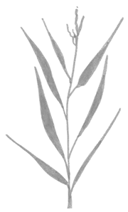 |
| Sa. and Sp. | Length of the second leaf from the top | 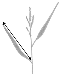 |
| Sa. and Sp. | Width of the petiole of the second leaf from the top |  |
| Sa. | Width of the second leaf from the top | 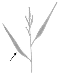 |
| Sp. | Stem count |  |
| Metrics | Species | Inundation Time | Inundation Time Squared | Nutrient | Pre-Condition | Channel (0—East, 1—West) | |||||
|---|---|---|---|---|---|---|---|---|---|---|---|
| 95% CI | 50% CI | 95% CI | 50% CI | 95% CI | 50% CI | 95% CI | 50% CI | 95% CI | 50% CI | ||
| Aboveground Biomass YR 1 | Sa. | - | + | + | + | - | - | ||||
| Sp. | - | - | + | + | + | + | - | - | |||
| Aboveground Biomass YR 2 | Sa. | + | + | - | + | + | - | ||||
| Sp. | - | + | + | ||||||||
| Belowground Biomass YR 1 | Sa. | + | - | + | - | - | |||||
| Sp. | - | ||||||||||
| Belowground Biomass YR 2 | Sa. | + | + | - | + | + | - | ||||
| Sp. | - | - | + | + | |||||||
| Year 1 (4 months) | Year 2 (16 months) | ||||||||
|---|---|---|---|---|---|---|---|---|---|
| Metrics | Species | Inundation Time | Inundation Time Squared | Inundation Time | Inundation Time Squared | ||||
| 95% CI | 50% CI | 95% CI | 50% CI | 95% CI | 50% CI | 95% CI | 50% CI | ||
| Plant Height | Sa. | + | + | - | + | + | - | - | |
| Sp. | - | - | - | ||||||
| Leaf Count | Sa. | - | - | + | - | ||||
| Sp. | - | - | - | ||||||
| Leaf Length | Sa. | - | + | + | - | ||||
| Sp. | + | - | - | + | + | ||||
| Stem Width | Sa. | + | + | + | |||||
| Sp. | + | - | - | ||||||
| Leaf Width | Sa. | + | + | + | - | ||||
| Stem Count | Sp. | + | + | - | - | + | |||
| Year 1 (4 months) | Year 2 (16 months) | ||||
|---|---|---|---|---|---|
| Metrics | Species | Nutrient | Nutrient | ||
| 95% CI | 50% CI | 95% CI | 50% CI | ||
| Plant Height | Sa. | + | + | ||
| Sp. | + | + | |||
| Leaf Count | Sa. | * | * | + | + |
| Sp. | + | + | + | + | |
| Leaf Length | Sa. | + | + | + | + |
| Sp. | + | + | + | ||
| Stem Width | Sa. | + | + | + | + |
| Sp. | + | + | + | ||
| Leaf Width | Sa. | + | + | + | + |
| Stem Count | Sp. | + | + | ||
| Year 1 (4 months) | Year 2 (16 months) | ||||
|---|---|---|---|---|---|
| Metrics | Species | Pre-Condition | Pre-Condition | ||
| 95% CI | 50% CI | 95% CI | 50% CI | ||
| Plant Height | Sa. | + | + | + | + |
| Sp. | + | + | + | + | |
| Leaf Count | Sa. | - | |||
| Sp. | + | + | |||
| Leaf Length | Sa. | + | + | ||
| Sp. | + | ||||
| Stem Width | Sa. | + | + | ||
| Sp. | + | ||||
| Leaf Width | Sa. | + | - | ||
| Stem Count | Sp. | + | + | - | - |
| Year 1 (4 months) | Year 2 (16 months) | ||||
|---|---|---|---|---|---|
| Metrics | Species | Days | Month Temp | ||
| 95% CI | 50% CI | 95% CI | 50% CI | ||
| Plant Height | Sa. | - | - | ||
| Sp. | - | - | |||
| Leaf Count | Sa. | + | + | + | |
| Sp. | + | + | |||
| Leaf Length | Sa. | - | - | ||
| Sp. | + | ||||
| Stem Width | Sa. | - | |||
| Sp. | + | ||||
| Leaf Width | Sa. | + | |||
| Stem Count | Sp. | + | |||
| Year 1 (4 months) | Year 2 (16 months) | ||||
|---|---|---|---|---|---|
| Metrics | Species | Channel | Channel | ||
| 95% CI | 50% CI | 95% CI | 50% CI | ||
| Plant Height | Sa. | - | - | ||
| Leaf Count | Sa. | + | - | - | |
| Leaf Length | Sa. | - | - | - | - |
| Stem Width | Sa. | - | - | ||
| Leaf Width | Sa. | - | |||
Disclaimer/Publisher’s Note: The statements, opinions and data contained in all publications are solely those of the individual author(s) and contributor(s) and not of MDPI and/or the editor(s). MDPI and/or the editor(s) disclaim responsibility for any injury to people or property resulting from any ideas, methods, instructions or products referred to in the content. |
© 2025 by the authors. Licensee MDPI, Basel, Switzerland. This article is an open access article distributed under the terms and conditions of the Creative Commons Attribution (CC BY) license (https://creativecommons.org/licenses/by/4.0/).
Share and Cite
San Antonio, K.M.; Wu, W.; Holifield, M.; Huang, H. The Impact of Inundation and Nitrogen on Common Saltmarsh Species Using Marsh Organ Experiments in Mississippi. Water 2025, 17, 1504. https://doi.org/10.3390/w17101504
San Antonio KM, Wu W, Holifield M, Huang H. The Impact of Inundation and Nitrogen on Common Saltmarsh Species Using Marsh Organ Experiments in Mississippi. Water. 2025; 17(10):1504. https://doi.org/10.3390/w17101504
Chicago/Turabian StyleSan Antonio, Kelly M., Wei Wu, Makenzie Holifield, and Hailong Huang. 2025. "The Impact of Inundation and Nitrogen on Common Saltmarsh Species Using Marsh Organ Experiments in Mississippi" Water 17, no. 10: 1504. https://doi.org/10.3390/w17101504
APA StyleSan Antonio, K. M., Wu, W., Holifield, M., & Huang, H. (2025). The Impact of Inundation and Nitrogen on Common Saltmarsh Species Using Marsh Organ Experiments in Mississippi. Water, 17(10), 1504. https://doi.org/10.3390/w17101504