Development of Flood Early Warning Framework to Predict Flood Depths in Unmeasured Cross-Sections of Small Streams in Korea

Abstract

Climate changes have increased heavy rainfall, intensifying flood damage, especially along small streams with steep slopes, fast flows, and narrow widths. In Korea, nearly half of flood-related casualties occur in these regions, underscoring the need for effective flood early warning systems. However, predicting flood depths is challenging due to the complex channels and rapid flood wave propagation in small streams. This study developed a flood early warning framework (FEWF) tailored for small streams in Korea, optimizing rainfall–discharge nomographs using hydro-informatic data from four streams. The FEWF integrates a four-parameter logistic model with real-time updates with a nomograph using a robust constrained nonlinear optimization algorithm. A simplified two-level early warning system (attention and severe) is based on field-verified thresholds. Discharge predictions estimate the water depth in unmeasured cross-sections using the Manning formula, with real-time data updates allowing for the dynamic identification of the flood depth. The framework was validated during the 2022 flood event, where no inundation or bank failures were observed. By improving flood prediction and adaptive management, this framework can significantly enhance disaster response and reduce casualties in vulnerable small stream areas.

1. Introduction

Climate change has significantly altered precipitation patterns in Korea, leading to an increase in extreme weather events. Over the past century, the average annual precipitation has risen by 135.4 mm, while the number of rainy days has decreased by 21.2. According to the Korea Meteorological Administration (KMA), future projections indicate that between 2021 and 2100, the intensity of rainfall in Korea’s metropolitan cities will increase significantly compared to that in the period from 2000 to 2019 [1]. This shift is expected to result in less frequent but more intense rainfall events, thereby elevating the risk of torrential rainfall.

Over the past decade, communities with low climate resilience, defined as the ability to withstand climate change impacts, have experienced flood- and typhoon-related mortality rates 15 times higher than those of more resilient communities [2]. More than 86% of damage from natural disasters in Korea is caused by extreme rainfall such as torrential rain or typhoons [3]. This low-frequency but intense torrential rainfall increases the flood damage around rivers and acts as an immediate physical threat to those affected. The effects of flooding persist over a long period of time and has the greatest impact on vulnerable communities. In particular, small streams located upstream of rivers typically have small watershed areas and steep slopes. Their narrow channels make them highly vulnerable to flooding. These streams also face a high risk of collapse and loss. Therefore, it is urgent to develop adaptation measures to reduce damage to these small streams.

Recent research has shown that climate change is still a major factor influencing changes in flood runoff. However, the impact of human activities has grown significantly in recent decades. For example, studies in the Hanjiang River basin in China (1960–2019) showed that climate change accounted for about 21% of runoff variations, while human activities contributed to around 79% [4]. Flooding is often caused by complex inter-connections between rivers and small streams that occur over various timescales depending on the sub-catchment scale and land use [5,6,7,8,9,10,11]. Small streams are critical in reducing the peak flood discharge within a watershed, effectively increasing the lag time between the peak rainfall and peak flood discharge in downstream rivers [6,12,13]. In other words, unmanaged land use changes in small stream watersheds can cause peak flood discharges to occur at the same time. Similarly, modifying small streams to increase their flood volume can have the same effect. These changes can lead to a significant rise in the maximum flood discharge in downstream rivers. Therefore, since small streams greatly affect the flooding of streams and rivers located in the lower part of watersheds, caution is needed in planning structural or non-structural changes.

Watersheds at higher elevations, such as small stream watersheds, are especially vulnerable to rapid increases in the peak flood discharge. This is due to several factors: (i) increased rainfall in high-altitude areas; (ii) a small watershed size and narrow waterways that are more sensitive to extreme rainfall; and (iii) a high likelihood of runoff synchronization within the watershed [14]. In Korea, small streams have an average channel width of 15.80 m and an average bed slope of 0.06. In these streams, the lag time is mainly influenced by the watershed slope. Other factors such as the stream network configuration, channel morphology, and bed conditions play a smaller role [6,9,15]. Furthermore, implementing flood control measures in small stream watersheds where such measures are relatively easy to carry out can effectively contribute to reducing river flooding [16,17].

Thus, ensuring the effective flood response of rivers located downstream requires the ability to accurately predict upstream small stream floods so that changes in the downstream flow can be detected quickly and solutions can be prepared in advance. Community-based adaptation measures supported by flood forecasting data are essential for reducing flood damage exacerbated by climate change and sustainably managing small streams. To prepare a sustainable plan under climate change, it is important to develop technology suited to local conditions or watershed characteristics. This technology should then be applied at actual sites for verification. Securing measured data from the sites must be a priority to ensure accurate verification. Since 2016, the National Disaster Management Research Institute (NDMRI) in Korea has implemented CCTV-based automated discharge measurement technology (CADMT) in small streams to measure real-time hydrodynamic data [18,19]. CADMT is a type of surface image velocimeter developed by the NDMI in Korea in 2016. Its accuracy and reliability were evaluated through extensive experiments in small streams, open channels, and artificial channels [18,19]. Furthermore, since 2023, the Ministry of the Interior and Safety, Korea, together with local governments, has been establishing smart monitoring systems in 2200 small streams, which constitute 10% of all small streams in Korea, to measure hydrodynamic data [19]. These systems typically measure velocity profiles and water depths to determine the flow discharges at one measurement cross-section per small stream, determined by using the ISO standards [20,21].

This research developed a flood early warning framework (FEWF) to minimize human casualties in areas near small streams, where about 42.3% of human casualties caused by natural disasters occur in Korea. As objective functions for optimization, the FEWF used rainfall–discharge nomographs developed using hydrodynamic data measured by using CADMT in small streams. The developed FEWF is an interlocking model that updates rainfall–discharge nomographs in real time using measured data. It does not require rebuilding, even if the predicted discharge falls outside the original range of the nomograph. The FEWF predicts the real-time flood water depth using the Manning formula in small streams including unmeasured cross-sections to define the flood depth of the sections and to support adaptive management solutions for each section. The developed FEWF was evaluated by comparing its predicted flow discharges and depths with measured values. These measurements were collected at the cross-sections of four small streams: the Jungsunpil, Sunjang, Neungmac, and Insu streams. The research also evaluated the applicability of the FEWF by comparing the predictive results with the levee height of small streams to analyze whether there were cross-sections demonstrating an overflow or bank collapse during the 2022 flood event. During the 2022 flood, no flood sections were observed in the small streams. The prediction results also showed no levee overflows or bank collapse. Therefore, the developed FEWF can be used to predict the water depth at the unmeasured cross-sections of small streams.

2. Materials and Methods

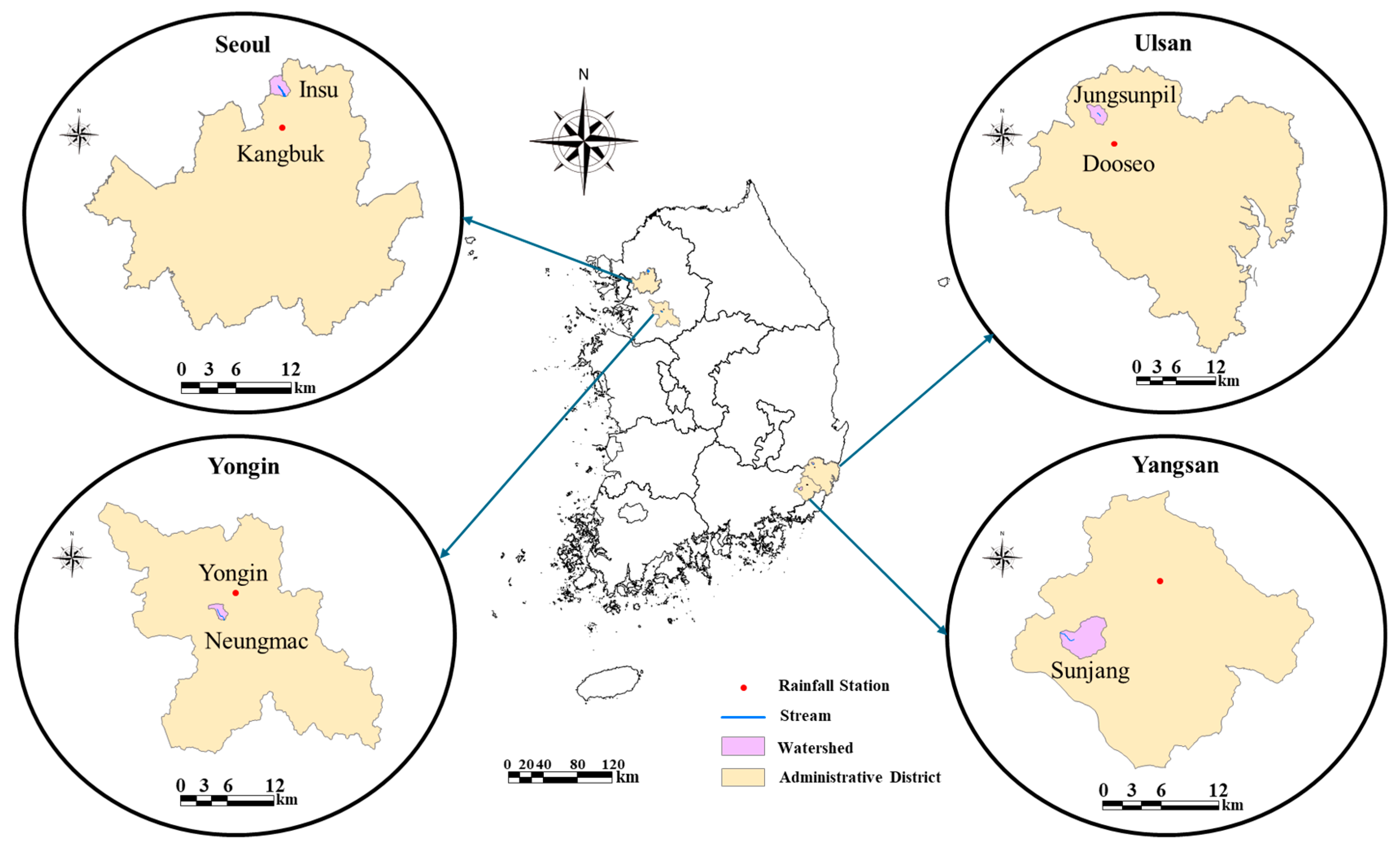
2.1. Selection of Small Streams

To develop real-time flood depth prediction technology for unmeasured small stream cross-sections, the discharges predicted by the FEWF at gauged sections were used. Four small streams were selected for this purpose: the Jungsunpil stream in Ulsan, Sunjang stream in Yangsan, Neungmac stream in Yongin, and Insu stream in Seoul, Korea, as shown in Figure 1. Since these four small streams have been measured using CADMT since 2016, we selected them to develop and evaluate the framework using measured hydrodynamic data. The research collected the rainfall, water depth, and discharge data in minutes measured using CADMT for seven years from 2016 to 2022.

The key characteristics of the watersheds and channels for these four small streams are summarized in

Table 1. Comparisons of small stream locations and main characteristics of small stream watersheds and channels.

Small Stream	Latitude	Longitude	${\mathit{A}}_{\mathit{b}}$ (km2)	${\mathit{W}}_{\mathit{b}}$ (km)	${\mathit{C}}_{\mathit{b}}$	${\mathit{S}}_{\mathit{c}}$	${\mathit{L}}_{\mathit{c}}$ (km)	${\mathit{W}}_{\mathit{c}}$ (m)	$\mathit{n}$
Jungsunpil	35.65.17 N	129.13.17 W	5.09	1.60	0.50	0.096	3.18	14.00	0.066
Sunjang	35.24.04 N	128.55.49 W	13.63	2.17	0.34	0.093	2.14	33.50	0.130
Neungmac	37.24.31 N	127.16.81 W	2.41	0.78	0.25	0.054	3.09	9.450	0.190
Insu	37.40.20 N	127.00.20 W	3.66	1.17	0.38	0.025	3.12	17.06	0.225

. Among the selected streams, the Jungsunpil and Sunjang streams are located in mountainous regions and have relatively steep slopes, while the Neungmac and Insu streams are located in urban areas with more gradual slopes.

Table 1 shows that the Sunjang stream had the largest watershed area, $A_b$, at 13.63 km², whereas the Insu stream had the smallest at 3.66 km². The average channel width, $W_b$, ranged from 0.78 to 2.17 km, classifying the streams as relatively narrow. The shape factors, $C_b=A_b/L_b^2$, which indicated elongated watershed geometries, with the watershed length denoted as $L_b$, ranged between 0.25 and 0.5. The streams had an average channel slope, $S_c$, of 0.067, an average stream length, $L_c$, of 2.88 km, and an average width, $W_c$, of 18.50 m, further supporting their classification as narrow and elongated streams. Manning’s roughness coefficients, $n$, required to solve the Manning formula, ranged from 0.066 to 0.225 and were determined from the survey and observation data for each small stream. The average river slope, $S_c$, of the four studied small streams ranged from 0.025 to 0.096, with an average of 0.067. The channel lengths, $L_c$, were relatively short, ranging from 2.13 to 3.18 km, and the widths, $W_c$, were narrow, ranging from 9.45 to 33.50 m.

2.2. Selection of Weather Stations

To obtain rainfall data that reflected the runoff characteristics of the small streams, a correlation analysis was performed. This analysis compared detailed observation data from the Korea Meteorological Administration’s (KMA) automatic weather system (AWS) with the runoff from the small streams (Figure 1) [18]. The analysis indicated that, for all the small streams except the Insu stream in Seoul, the nearest AWS stations exhibited the highest correlation with the runoff. Accordingly, rainfall data from these stations were used to develop discharge prediction technology and perform verification for the FEWF.

For the Insu stream, the rainfall data from the Kangbuk AWS, which demonstrated the highest correlation with the runoff from the Insu stream, were selected for development and evaluation. The relevant attributes of the selected AWSs are summarized in

Table 2. Information on the characteristics of the selected rainfall gauging stations in each small stream watershed.

Small Stream	AWS	Latitude	Longitude	$\mathit{E}$ ($\mathbf{E}\mathbf{L}.\mathbf{m}$)	$\mathit{D}$ ($\mathbf{k}\mathbf{m}$)	${\mathit{R}}_{\mathit{a}}$ ($\mathbf{m}\mathbf{m}$)	${\mathit{Y}}_{\mathit{s}}$
Jungsunpil	Dooseo	35.62.03 N	129.14.35 W	123	4.23	1274	1991
Sunjang	Yangsan	35.30.74 N	129.02.01 W	6.29	9.86	1588	2008
Neungmac	Yongin	37.27.01 N	127.22.18 W	83.0	5.83	1293	2005
Insu	Kangbuk	37.73.50 N	127.07.50 W	72.0	10.4	1544	2001

, including their locations; elevations, $E$; distances, $D$, to the streams; average annual rainfall, $R_a$; and observation start years, $Y_s$. In Table 2, it can be seen that the average annual rainfall recorded at the streams ranged from 1274 mm to 1588 mm, with the majority of precipitation concentrated between June and September, coinciding with the summer monsoon season.

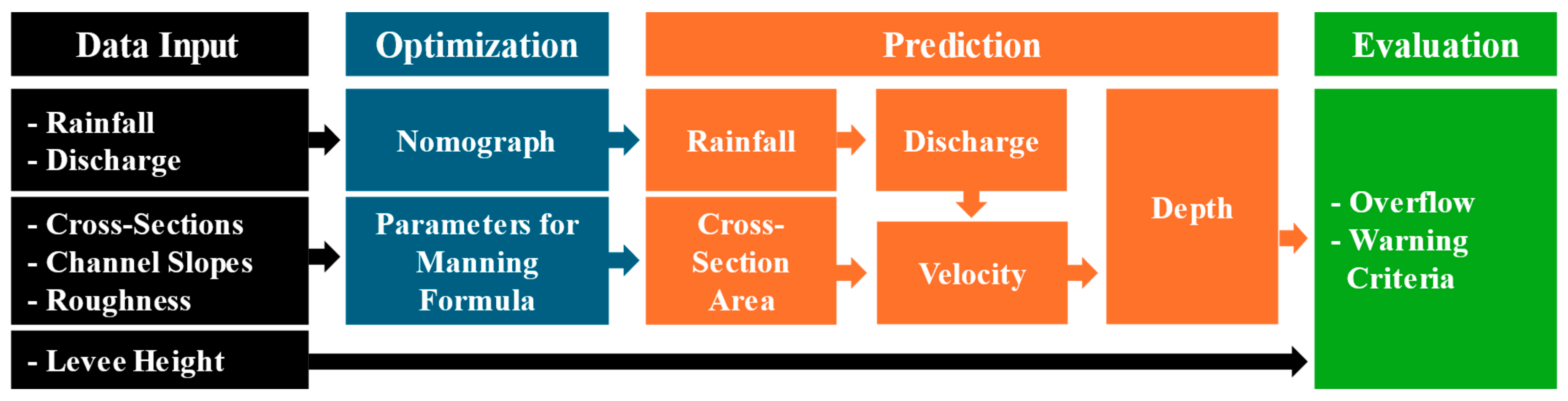
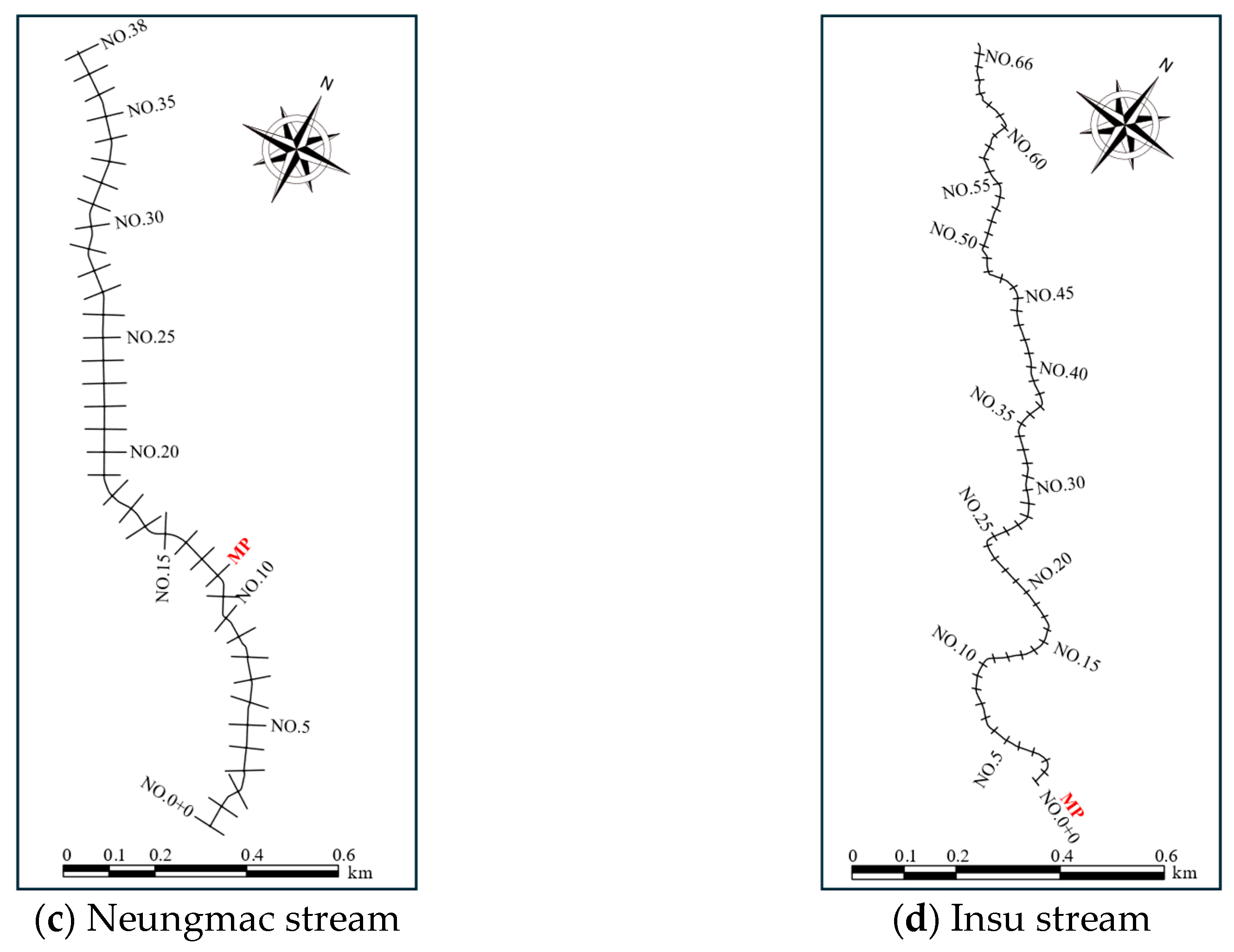
2.3. Flood Depth Prediction Method for Unmeasured Cross-Sections and Data Collection

The real-time discharges and depths for small streams can be predicted using various approaches. These include numerical model-based simulations evaluated using historical data [22,23,24,25], artificial intelligence (AI)-based optimization techniques using real-time measurement data [19,26], and remote feedback modeling technologies that control measurement and imaging equipment [27,28,29]. The numerical model-based prediction methods involve developing and evaluating models by using measured depths, discharges, and rainfall data to predict the flood discharge and water depth. While effective within a validated range, these models require reevaluation to predict larger floods outside that range [30]. Numerical models require an evaluation process that involves establishing a model using geographic and cross-sectional data. Additionally, the optimal parameters must be determined to predict flood discharges and water depths based on the predicted rainfall. These models can predict accurate results within the evaluated range but can be challenging to apply in the event of large floods outside the validation range.

On the other hand, AI-based optimization techniques can modify their object functions using measured data in real time, so an additional evaluation process is not required for conditions outside the validated range. However, these techniques are not suitable for application to rivers or sections of them without hydrodynamic data measured in real time. Their limitation is that they can only be used when information measured in real time is available. This research aimed to develop an FEWF to predict the depths at unmeasured small stream cross-sections using the measured section discharges under the assumption that there is no change in the stream flow due to there being no inflow from a tributary. Figure 2 shows the procedure for predicting water depths by using the FEWF.

In Figure 2, it can be seen that the discharges were predicted by using a rainfall–discharge nomograph with predicted rainfall data obtained by using the McGill algorithm for precipitation nowcasting (MAPLE) [31,32,33]. This research developed a rainfall–discharge nomograph based on historical data measured for the four small streams listed in

Table 3. Characteristics of data measured for 7 years from 2016 to 2022 for four small streams used to develop and evaluate the FEWF.

Use Type	Small Stream	R ($\mathbf{m}\mathbf{m}$)		H ($\mathbf{m}$)		Q (${\mathbf{m}}^3/\mathbf{s}$)		HL ($\mathbf{m}$)
		Mean	Max	Mean	Max	Mean	Max	Min	Max
Development (2016~2021)	Jungsunpil	0.16	80.0	0.24	1.98	0.83	28.78	1.87	12.58
	Sunjang	0.19	95.8	0.40	2.45	1.32	210.3	2.98	9.67
	Neungmac	0.15	55.5	0.18	1.65	0.15	14.13	2.15	15.17
	Insu	0.17	51.5	0.23	1.39	0.09	21.39	1.38	12.10
Evaluation (2022)	Jungsunpil	0.16	84.8	0.11	1.61	0.08	35.93	1.87	12.58
	Sunjang	0.17	59.3	0.20	1.64	0.85	65.19	2.98	9.67
	Neungmac	0.17	56.7	0.14	1.74	0.14	14.41	2.15	15.17
	Insu	0.30	62.5	0.21	2.52	0.24	68.88	1.38	12.10

, in which the zero values measured during dry seasons when the small streams were nearly dry were not included in the minimum value. The discharges were used as initial values to predict the depth in unmeasured sections of the small streams using the Manning formula. To predict the depth using the Manning formula, the cross-sectional area was assumed by using the estimated cross-sectional depth to calculate the velocity as the input value, and then the discharges were estimated. The estimated discharges were compared with the initially input predicted discharges to calculate the error and the procedure was repeated until the error was minimized to determine the depth at which the error was minimized. If the predicted depth exceeded the warning criteria, a warning would be issued. Measured rainfall and hydraulics data collected for 6 years from 2016 to 2021 for four small streams were used for the development of the FEWF, and the data measured in 2022 were used for the evaluation.

To predict the flood depth for an unmeasured section using the Manning formula, cross-sectional information for each section was extracted from the field survey results, as shown in Figure 3. Manning’s roughness coefficients and the channel slope, as shown in Table 1, were determined from the survey and observation results for each small stream. The cross-sectional information obtained at the measurement point for each of the four small streams, shown as MP in Figure 3, is plotted in Figure 4.

3. The Development of the Small Stream Flood Early Warning Framework

This research performed two major steps in the development of an FEWF, prediction and evaluation, as illustrated in Figure 5. The first step involved the development of a rainfall–discharge nomograph (NG) using historical rainfall, $R_H$, and discharge, $Q_H$, data collected, respectively, from the AWS and from the small stream by using CADMT to predict the discharge. In this step, the predicted rainfall, $R_P$, was obtained by using the MAPLE, which used Lagrangian Extrapolation to predict the discharges. The predicted discharge, $Q_P$, was compared with the recently measured discharge, $Q_M$, in the first step to determine whether to enhance the rainfall–discharge nomograph with values of the rainfall and discharge measured in real time. If the residual between the predicted and measured values met the convergence criteria, the prediction of the discharge was finished. If it did not meet the criteria, the rainfall–discharge nomograph could be updated with newly measured discharge and rainfall data.

The second step involved predicting the depth by using the Manning formula and evaluating whether the predicted depth, $H_P$, would exceed the warning criteria, $C_W$. To predict the depth, the cross-sectional area and hydraulic radius were estimated by using the measured cross-section, $C_M$, and the estimated depth, $H_E$, and then the discharge was estimated by multiplying the assumed area and estimated velocities, $V_E$, determined by using parameters such as the measured slope, $S_M$, and Manning’s roughness, $n$. The estimated discharge, $Q_E$, was then compared with the predicted discharge, $Q_P,$ to determine whether to estimate the depth. If the residual between the predicted and estimated values met the convergence criteria, the estimation was finished to predict the depth. The predicted depth was used to determine whether it would exceed the warning criteria, $C_W$. If the predicted depth exceeded the warning criteria, a flood warning would be issued to evacuate people from hazardous areas, including those near small streams. If it did not exceed the warning criteria, the discharge and depth prediction process could be continued without updating the rainfall–discharge nomograph to predict the rainfall for the next time step. This research used the robust constrained nonlinear optimization algorithm (RCNOA) to enhance the rainfall–discharge nomograph by minimizing the root mean square error (RMSE) between the predicted and measured sets of normalized data.

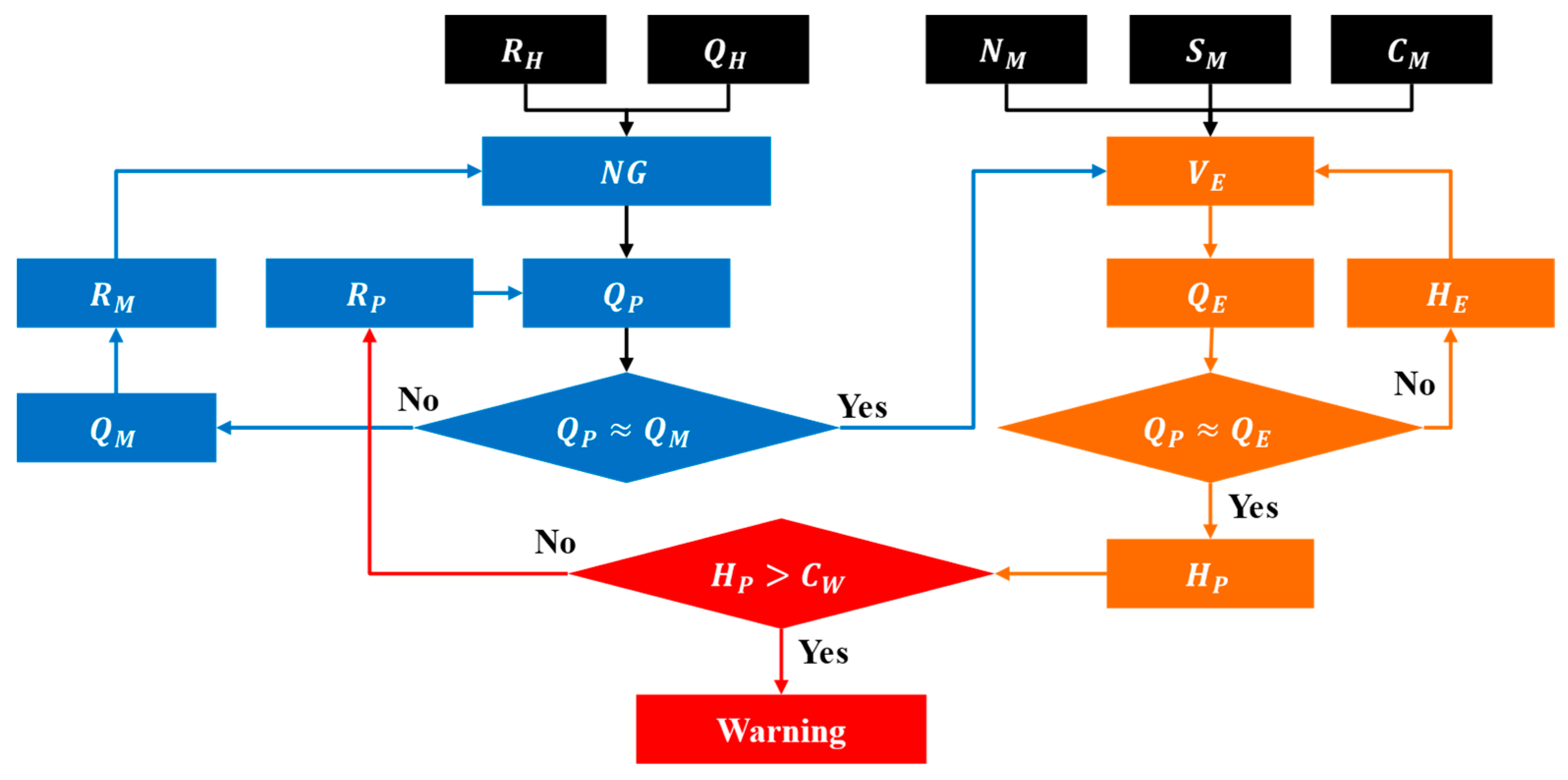
3.1. Real-Time Flood Discharge Prediction Technology

To predict the flood discharge, this research developed a rainfall–discharge nomograph using historical rainfall and discharge data measured for the four studied small streams over six years from 2016 to 2021. A rainfall–discharge nomograph is a statistical tool that graphically represents the relationship between the rainfall and discharge, a widely used tool for discharge forecasting [19,34,35,36]. Historical data analysis has shown that rainfall–discharge nomographs take the form of an S-curve with a gradual increase in the low-discharge section, a sharp increase in the medium-discharge section, and a gradual increase in the high-discharge one. The nonlinear four-parameter logistic (4PL) method, also known as the Hill model, has been shown to effectively reproduce this S-curve-shaped data distribution [37,38]. Therefore, this research developed a rainfall–discharge nomograph using the 4PL method, as shown in the following equation:

$$NG=f\left(R_{H\_60t}|qm\right)={qm}_1+{\displaystyle \frac{{qm}_2-{qm}_1}{1+{\left(R_{H\_60t}/{qm}_3\right)}^{{qm}_4}}},$$

(1)

in which $R_{H_{60t}}$ is the cumulative rainfall measurement, with this research analyzing the cumulative rainfall over 60 min, and ${qm}_1, q{m}_2, q{m}_3, \mathrm{a}\mathrm{n}\mathrm{d} q{m}_4$ are the optimal parameters with which the residual sum of squares was minimized. This research used historical peak discharge values, determined using the following equation:

$$Q_{H\_max}=max\left|{{Q_H(I}_s)~Q_H(I}_e)\right|,$$

(2)

in which $I_s$ is the start time, defined as $\left[I_t, { I}_{t+2}, \dots ,{ I}_{k-1}\right]$, $I_e$ is the end time, defined as ${[I}_{t+1}, { I}_{t+3}, \dots ,{ I}_k]$, $I_t$ is the observed rainfall event start time, and $I_k$ is the observed rainfall event end time. This research used the RCNOA to develop a rainfall–discharge nomograph. The variables of the 4PL function were determined using only values within a statistically useful range [19,39,40,41]. To develop an $NG$ with a 95% confidence interval, this research removed the outliers by applying the Studentized Deleted Residual, as shown in the following equation:

$$SDR={\epsilon }_i{\left[{\displaystyle \frac{l-d-1}{SSE(1-h_{ii}-{\epsilon }_i^2)}}\right]}^{1/2},$$

(3)

in which ${\epsilon }_i$ is the $i$th residual, $l$ is the amount of observation data, $d$ is the number of regression coefficients, $SSE$ is the sum squared error, and $h_{ii}$ is the $i$th diagonal element. The resulting rainfall–discharge nomographs developed are shown in Figure 6, along with the measured data for all four small streams.

The optimized parameters and the coefficient of determination for each rainfall–discharge nomograph are summarized in

Table 4. Comparison of the results for the optimum parameters for the rainfall–discharge nomographs optimized by using the RCNOA and the coefficients of determination for each small stream.

Small Stream	Optimum Parameters				Coefficient of Determination (${\mathit{R}}^2$)
	${\mathit{q}\mathit{m}}_1$	${\mathit{q}\mathit{m}}_2$	${\mathit{q}\mathit{m}}_3$	${\mathit{q}\mathit{m}}_4$
Jungsunpil	49.286	1.5220	15.808	1.8832	0.98
Sunjang	316.28	7.6866	44.553	2.8078	0.99
Neungmac	288.92	1.0491	86.824	4.2870	0.99
Insu	60.758	1.8662	62.927	3.3865	0.99

. The coefficient of determination ranged from 0.98 for the Jungsunpil stream to 0.99 for the other small streams. This indicates that the developed rainfall–discharge nomographs accurately represent the relationship between the rainfall and discharge runoff in small streams.

To predict the discharge using the developed rainfall–discharge nomographs, this research used the MAPLE-forecasted rainfall provided by the KMA as an input value. If the time interval of the previously observed rainfall data, $∆t$, was one minute, the total measured rainfall set, $R_{∆t}$, was defined as $\left\{R_t|R_t, t=∆t,2∆t,3∆t, \cdots , N\right\}$, and the cumulative rainfall over 60 min, $R_{H\_60t}$, was as follows:

$${\sum }_t^j{R}_{H\_60t},t=0,∆t,2∆t,3∆t,\cdots ,j \mathrm{i}\mathrm{f} t\le 60 \min ,$$

(4)

$$\sum _t^N{R}_{H\_60t},t=j-60,j+∆t,j+2∆t,\cdots ,N,j \mathrm{i}\mathrm{f} t>60 \min ,$$

(5)

If $R_{H\_60t}$ was greater than zero, the total rainfall measurement time was defined as $T_t=\left\{R_{H\_60t}|R_{H\_60t}>0\right\}$. If the rainfall measurement time interval was greater than zero, the total measurement time interval was defined as $I_t=\left\{T_t-T_{t-∆t}|T_t-T_{t-∆t}>∆t\right\}$. Assuming that the current time was $tpr$, the predicted discharge at time $k$, $Q_{tp{r}_{-}{P}_{-}cal-k}$, was determined by the following equation as

$$Q_{tp{r}_{-}{P}_{-}cal-k}={qm}_1+{\displaystyle \frac{{qm}_2-{qm}_1}{1+{\left(R_{60\_tpr-k}/{qm}_3\right)}^{{qm}_4}}},$$

(6)

in which $R_{60_{-}tpr-k}$ is the cumulative rainfall over 60 min $k$ hours ago. If the residuals between the predicted discharge $Q_p$ and the measured discharge $Q_m$ at time $k$ did not exceed the residual criterion, the $k+1$ step discharge was predicted without improving the rainfall–discharge nomograph. However, if the residual criterion was exceeded, the RCNOA-based optimization process would be repeated to reconstruct the rainfall–discharge nomograph by considering the measured $Q_m$ and $R_m$ at time $k$, and the $k+1$ time step discharge would be predicted [19]. This research defined the residual criterion tolerance as 0.03. In the case that this was exceeded, the rainfall–discharge nomograph was improved by considering the measured values, the optimal parameters determined for the $k+1$ time step were re-determined using the RCNOA, and the $k+1$ time step discharge, $Q_{tp{r}_{-}{P}_{-}cal-k+1}$, was predicted using the following equation as

$$Q_{tp{r}_{-}{P}_{-}cal-k+1}={qm}_{1_{-}md}+{\displaystyle \frac{{qm}_{2_{-}md}-{qm}_{1_{-}md}}{1+{\left(R_{{60}_{tpr}-k+1}/{qm}_{3_{-}md}\right)}^{{qm}_{4_{-}md}}}},$$

(7)

in which ${qm}_{1_{-}md}$, ${qm}_{2_{-}md}$, ${qm}_{3_{-}md}$, and ${qm}_{4_{-}md}$ are the newly determined optimal parameters used to improve the rainfall–discharge nomograph using the newly measured discharge and rainfall at time step $k$.

3.2. Robust Constrained Nonlinear Optimization Algorithm

This research used the RCNOA to improve the rainfall–discharge nomograph for predicting the discharge in real time. It also predicted the depth by using the Manning formula, aiming to minimize the residuals between the predicted and measured values in the small stream FEWF. The RCNOA is a robust method that minimizes the sum of residual functions that increase less rapidly than the sum of square errors [42]. The algorithm minimizes the sum of residual functions by using a correction vector, $\mathbf{\varnothing }$, defined as $\mathrm{m}\mathrm{i}\mathrm{n}\mathrm{\varnothing }=\mathrm{m}\mathrm{i}\mathrm{n}\left|\alpha {\mathbf{\theta }}^k/{\mathbf{\theta }}^k\right|$, in which the $\alpha$ is constant, and this research used 0.99 for the $\alpha$. The optimal parameters for the next time step were predicted by using constrained present time parameters and the following equation:

$${\mathbf{\theta }}^{k+1}={\mathbf{\theta }}^k+\mathrm{\varnothing }{\mathbf{\theta }}^k,$$

(8)

in which the constraint is $\left\{\mathbf{\theta }\right\}\ge 0$ and the iterative procedure can be continued until the sum of residual functions is minimized. The optimum parameters, $\mathbf{\theta }$, were calculated using the following equation as

$$\mathbf{\theta }=-\mathbf{P}{\left({\displaystyle \frac{\epsilon }{s}}\right)}^{\mathit{T}}s\mathbf{P}\left({\displaystyle \frac{\epsilon }{s}}\right)/\left[\mu \mathbf{I}+\mathbf{P}{\left({\displaystyle \frac{\epsilon }{s}}\right)}^{\mathit{T}}s\mathbf{P}\left({\displaystyle \frac{\epsilon }{s}}\right)\right],$$

(9)

in which $\mathbf{P}\left(·\right)$ is the Jacobian matrix of residual functions, $\mathbf{I}$ is the unit matrix, $s$ is the known or previously estimated scale parameters calculated using $1.48\mathrm{m}\mathrm{e}\mathrm{d}\left[\left|\epsilon -\mathrm{m}\mathrm{e}\mathrm{d}\left(\epsilon \right)\right|\right]$, where a coefficient of 1.48 is the value that results in an unbiased estimate of the scale parameter when the residual function is Gaussian [43], and $\mu$ is a nonnegative parameter estimated to be large enough to eliminate the singularity of the Jacobian matrix, represented as $\mathrm{m}\mathrm{a}\mathrm{x}\left|\mathbf{P}\left(·\right)\right|$. However, it is not too large to prevent it moving away from a specific region nearby at a reasonable rate. If $\left|\epsilon \right|$ is less than the 0.975 quartile square root of the residual, $\mathbf{P}\left(·\right)$ becomes $\epsilon$, and if $\left|\epsilon \right|$ is greater than the 0.975 quartile square root of the residual, $\mathbf{P}\left(·\right)$ becomes $\mathsf{\alpha }\mathrm{s}\mathrm{i}\mathrm{n}\left(\epsilon \right)$ [42].

3.3. Technology for Predicting Real-Time Flood Depth in Unmeasured Cross-Sections

This research simulated and analyzed the ability of various numerical models to estimate the flood depth of the unmeasured cross-sections of a small stream. The results showed that the existing unsteady flow models failed to provide stable results because small streams have steep and irregular slopes and complex geometry. Based on these findings, the Manning equation, which offers relatively stable solutions, was applied to predict the depth in the unmeasured cross-sections of the small streams. This research measured the transverse cross-sections of longitudinal sections of four small streams and divided them into sub-sections to consider complex changes in the cross-sectional area, hydraulic radius, and other relevant parameters for each sub-section. Assuming that the hydraulic slope of each sub-section was uniform, the discharges in the $i$th section were predicted using the following equation as

$$Q_i=A_i{V}_i={\displaystyle \frac{A_i{R}_i^{2/3}{S}_i^{1/2}}{n_i}},$$

(10)

in which $Q_i$ is the discharge in the longitudinal $i$th section, $A_i$ is the area of the longitudinal $i$th section, $V_i$ is the velocity in the longitudinal $i$th section, $R_i$ is the hydraulic radius of the longitudinal $i$th section, $S_i$ is the slope of the $i$th section, and $n_i$ is the Manning coefficient of the longitudinal $i$th section.

To predict the water depth in an unmeasured cross-section, this research used the predicted flood discharge, $Q_{tp{r}_{-}{P}_{-}cal-k-1}$, at time step $k$, using a rainfall–discharge nomograph as an input value for the Manning formula. For prediction, it was assumed that there was no tributary inflow into the small stream and the same discharge occurred consistently throughout the small stream along its longitudinal direction. To predict the water depth using Equation (10), the longitudinal $i$th section water level $H_i$ was initially assumed, the longitudinal $i$th section area $A_i$ was calculated, and then the longitudinal $i$th section velocity $V_i$ was determined using the following equation as

$$V_i=S_i^{1/2}{\sum }_{i=1}^N{\displaystyle \frac{r_{ij}^{2/3}}{n_{ij}}},$$

(11)

in which $r_{ij}$ is the transverse $i$th hydraulic radius of the longitudinal $i$th section, and $n_{ij}$ is the transverse $j$th roughness coefficient of the $i$th section. The longitudinal $i$th cross-sectional discharge obtained using Equation (11) was compared with the predicted discharge $Q_{tp{r}_{-}{P}_{-}cal-k-1}$ at time step $k$. If the residual between the predicted and obtained discharge values did not exceed the reference limit, the assumed water depth was determined to be the predicted longitudinal $i$th cross-sectional depth. However, if the residual exceeded the reference limit, the longitudinal $i$th cross-sectional water depth $H_i$ was reassumed. The process of calculating the discharge using Equation (11) was then repeated until the residual no longer exceeded the reference limit. In this research, the RCNOA-based optimization process was applied iteratively to determine the longitudinal $i$th cross-sectional water level.

3.4. Setting Flood Warning Criteria

This research categorized the warning levels into two distinct categories, a caution level and a severe level, as shown in Figure 7. Figure 7 shows that a caution-level warning would be issued when the predicted water depth was expected to exceed 0.5 m to warn the public to stay away from small streams. This threshold of 0.5 m was determined based on experimental studies by various researchers [44,45,46] which indicated the maximum depth that people can generally withstand. The severe-level warning would be issued when the water depth was anticipated to reach the design flood level as a warning to evacuate residents from areas near small streams to a safe location. The rationale for this simplification was that the four warning levels, an interest level, caution level, alert level, and severe level, commonly used in disaster response in Korea often led to the repeated issuance of caution and alert warnings within a short period, as observed in the case of the Sunjang stream flooding, shown in Figure 7. This redundancy could cause confusion among response officials. Moreover, the water depths in small streams typically rise rapidly, reaching a severe level within two hours of reaching the caution level, which makes a two-level system more efficient.

4. Results and Discussion

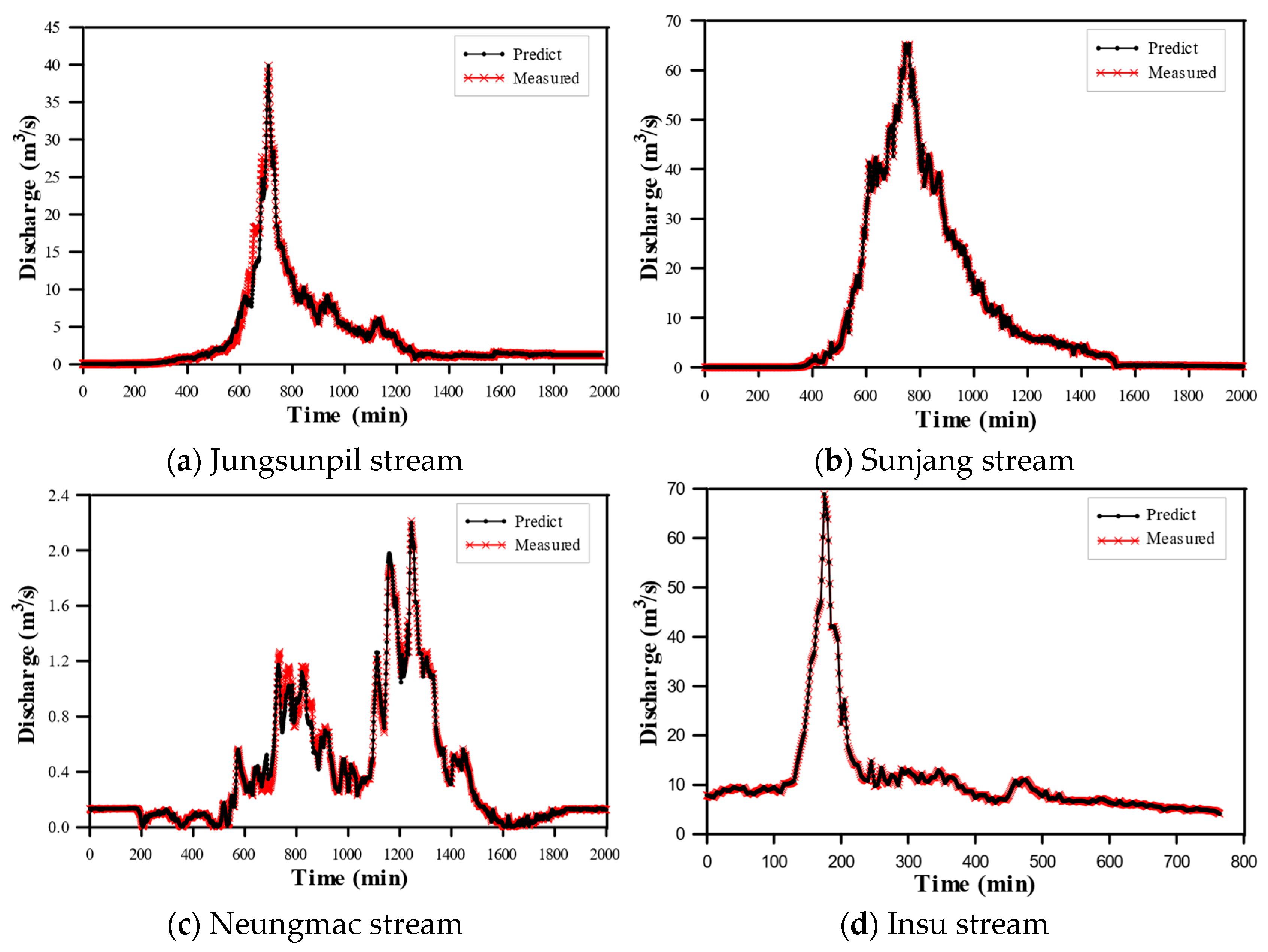
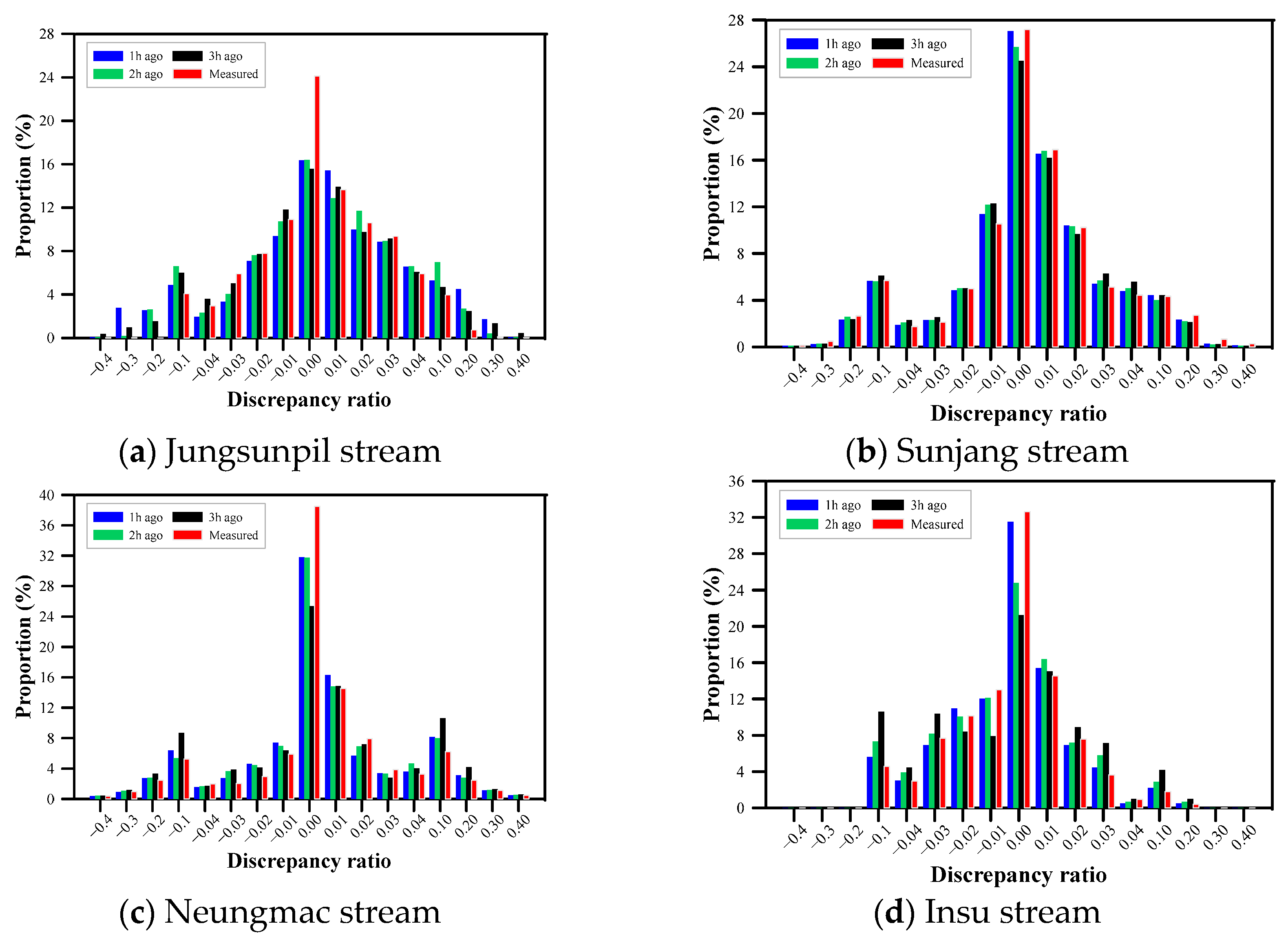
4.1. Discharge Prediction and Evaluation for Measured Small Stream Section

To implement a flood early warning system to reduce the casualties near small streams, it is very important to predict the flow discharge and depth before the flood occurs. To accomplish this, this research used the rainfall predicted using the MAPLE, provided by the KMA, to predict floods in advance. Since the MAPLE predicts rainfall in minutes by dividing the whole of Korea into 1 km grid intervals, this research used the grid values closest to the AWSs presented in Table 2 as the predicted rainfall values. To analyze the accuracy of the MAPLE’s prediction and evaluate the applicability of discharge and depth prediction, this research compared the rainfall predicted one, two, and three hours before with the rainfall measured by the AWSs selected in this research, and the comparison results are shown in Figure 8. For the evaluation, this research used rainfall and discharge data collected on August 9 for the Insu stream and September 5 for the other three small streams, days which corresponded to the largest flood events of 2022. Figure 8 shows that the predicted rainfall for the Jungsunpil stream and the Sunjang stream represented the measured rainfall distribution relatively well, but the predicted rainfall for the Neungmac stream and the Insu stream overestimated the rainfall.

To further evaluate the predicted rainfall’s impact on the discharge prediction results obtained using the rainfall–discharge nomograph, this research predicted the discharges using the FEWF and compared the predictions with values measured using CADMT for four small streams, as shown in Figure 9. The cumulative rainfall over 60 min was employed for predicting discharges in the four small streams, and it was found that the predicted results closely represented the measured time–discharge distributions of the four small streams, as shown in Figure 7.

To quantitatively evaluate the discharges predicted using the FEWF by inputting the rainfall predicted one, two, and three hours before, the root mean square error (RMSE) and maximum and minimum errors were compared, as shown in

Table 5. Comparison of the RMSE and maximum and minimum errors determined using the FEWF prediction results and discharges measured for four small streams: ${MR}_1$: rainfall predicted using the MAPLE one hour before; ${MR}_2$: rainfall predicted using the MAPLE two hours before; and ${MR}_3$: rainfall predicted using the MAPLE three hours before.

Small Stream	RMSE (${\mathbf{m}}^3/\mathbf{s}$)			Maximum Error			Minimum Error
	${\mathit{M}\mathit{R}}_1$	${\mathit{M}\mathit{R}}_2$	${\mathit{M}\mathit{R}}_3$	${\mathit{M}\mathit{R}}_1$	${\mathit{M}\mathit{R}}_2$	${\mathit{M}\mathit{R}}_3$	${\mathit{M}\mathit{R}}_1$	${\mathit{M}\mathit{R}}_2$	${\mathit{M}\mathit{R}}_3$
Jungsunpil	2.5	3.1	3.3	−38.1	−43.2	−36.0	−1.73	−2.46	−2.77
Sunjang	2.0	2.1	3.3	−13.8	−9.98	7.48	−1.76	−1.86	−1.48
Neungmac	1.3	1.7	2.0	−0.24	−1.08	0.38	−0.50	−1.08	−0.83
Insu	1.9	1.9	2.2	32.1	13.6	−18.7	−0.16	−1.64	−3.27
Mean	1.9	2.2	2.7	−5.01	−10.2	−11.7	−1.04	−1.76	−2.08

. The results for all the errors revealed that the discharge predicted using the MAPLE-predicted rainfall from one hour before best represented the measured values. The RMSE results for discharge prediction using the MAPLE-predicted rainfall from 1 h before revealed that the predictions for the Neungmac stream had the smallest value at 1.3, followed by those for the Insu stream and the Sunjang stream with values of 1.9 and 2.0, respectively, while those for the Jungsunpil stream showed the largest value at 2.5.

To more quantitatively evaluate the error between the measured and predicted values, this research calculated the discrepancy ratio, as proposed by White et al., 1972 [47]. The discrepancy ratio, $D_R$, was defined as $\mathrm{l}\mathrm{n}\left(V_p/V_m\right)$, in which $V_p$ represents the predicted value and $V_m$ signifies the measured value. When the discrepancy ratio was greater than 0, the predicted value overestimated the measured value, and if the discrepancy ratio was smaller than 0, the predicted value underestimated the measured value. A discrepancy ratio of 0 indicated that the predicted value aligned with the measured value. Furthermore, the closer the discrepancy ratio distribution was to a normal distribution, the less biased the predicted results were, and the more accurately the measured values were represented. To compare the distributions of the discrepancy ratios of the predicted discharges for the small streams, this research divided the part of the range from −0.04 to 0.04 into sections of 0.01, while the rest of the range was divided into sections of 0.1. The discrepancy ratio in each section was then plotted as a histogram, as shown in Figure 10.

The discrepancy ratios for discharge prediction in the small streams generally followed a normal distribution, suggesting that the FEWF represented the measured discharges effectively. The majority of the discrepancy ratios were distributed between −0.04 and 0.04, with the largest proportion falling between −0.01 and 0.01. The discrepancy ratios were most densely distributed around 0 for the Neungmac stream, followed by the Insu stream, the Sunjang stream, and the Jungsunpil stream. This research defined the range of discrepancies clustered between −0.003 and 0.003 as representing the accuracy. The accuracy results are summarized in

Table 6. Comparison of the accuracy of the discharge prediction results obtained by using the measured rainfall ($MR$) and the MAPLE-predicted rainfall from one, two, and three hours before.

Small Stream	Accuracy
	$\mathit{M}\mathit{R}$	${\mathit{M}\mathit{R}}_1$	${\mathit{M}\mathit{R}}_2$	${\mathit{M}\mathit{R}}_3$
Jungsunpil	67.08	58.24	59.37	58.85
Sunjang	69.87	70.25	70.06	67.76
Neungmac	69.89	65.84	64.95	57.91
Insu	77.97	76.86	70.60	61.48
Mean	71.20	67.80	66.25	61.50

. The highest accuracy in the discharge prediction results obtained by using the MAPLE-predicted rainfall from one hour before was observed for the Insu stream at 76.86%, followed by the Sunjang stream at 70.25%, the Neungmac stream at 65.84%, and finally the Jungsunpil stream at 58.24%. The accuracy results revealed that the discharges predicted using the MAPLE-predicted rainfall from one hour before best represented the measured values.

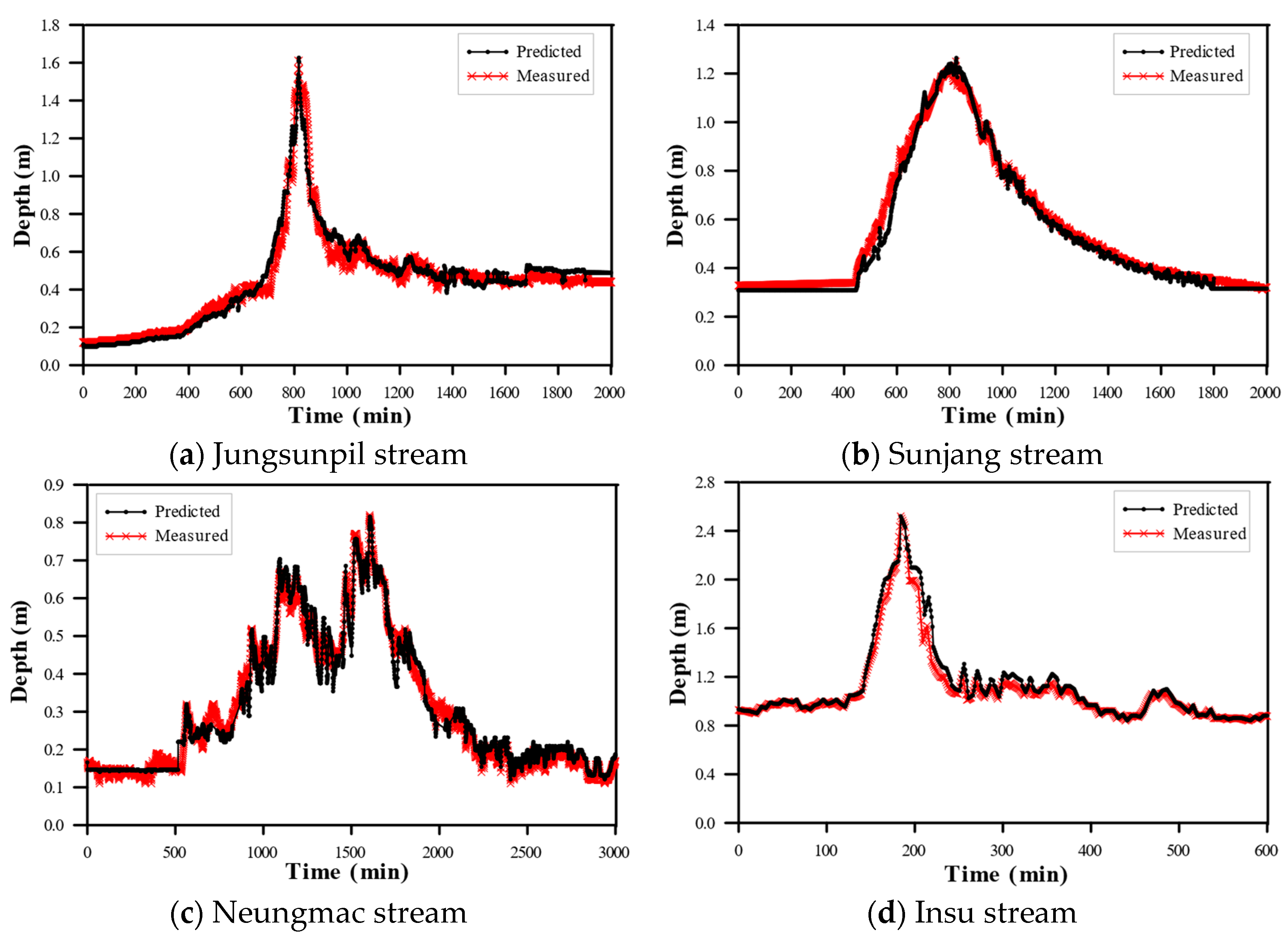
4.2. The Depth Prediction and Evaluation for Unmeasured Small Stream Sections

This research used the Manning formula to predict the depths using the FEWF by inputting the predicted discharges from one hour before for unmeasured cross-sections of the four small streams. To evaluate its applicability, the depths predicted by using the Manning formula for the four small streams were compared with the measured depths, as shown in Figure 11.

Figure 11 shows that the measured time–discharge distribution in the Neungmac stream showed a significant change with the rainfall, while the measured depth change with a discharge change was relatively small as the Neungmac stream had a compound cross-sectional shape, as shown in Figure 4c. It was found that the discharges decreased significantly during the time when the rainfall decreased, while the water depth decreased relatively little. Unlike the other three small streams, the Neungmac stream was estimated to have relatively little change in its depth compared to the change in its discharge, as a small stream with a complex cross-sectional shape. To quantitatively evaluate the depths predicted using the FEWF by inputting the predicted discharges from one hour before, the RMSE and the coefficient of determination were compared, as shown in

Table 7. Comparisons of Root Mean Square Error and coefficient of determinant calculated by using the FEWS prediction results and measured data from four test small streams.

Small Stream	RMSE	Coefficient of Determination
Jungsunpil	0.042	0.98
Sunjang	0.024	0.99
Neungmac	0.023	0.99
Insu	0.056	0.97
Mean	0.031	0.98

. The RMSE results revealed that the predictions for the Neungmac stream had the smallest value at 0.023, followed by those for the Sunjang stream and the Jungsunpil stream with values of 0.024 and 0.042, respectively, while those for the Insu stream showed the largest value at 0.056. The coefficient of determination results showed that the predictions for the Neungmac and Sunjang streams had the largest values at 0.99, followed by those for the Jungsunpil stream and the Insu stream with values of 0.98 and 0.97, respectively.

To more quantitatively evaluate the error between the measured and predicted values, this research calculated the discrepancy ratio and divided the discrepancy ratio range of −0.4 to 0.4 into intervals of 0.05 and visualized the distributions as histograms, shown in Figure 12. The proportion of discrepancy ratios concentrated within the range of −0.05 to 0.05 was defined as the accuracy of water depth prediction using the FEWF. The comparison results show that the predictions for the Sunjang stream and Insu stream exhibited discrepancy ratio distributions resembling normal distributions, indicating a good reproduction of the measured water levels over time. However, the predictions for the Jungsunpil stream and Neungmac stream showed an underestimation of the water levels in some segments, particularly when they were outside the peak water levels.

The accuracy results showed that the predictions for the Insu stream had the highest accuracy value of 95.63%, followed by those for the Neungmac stream and the Sunjang stream, with values of 91.61% and 90.15%, respectively, while those for the Jungsunpil stream showed the lowest value at 87.22%.

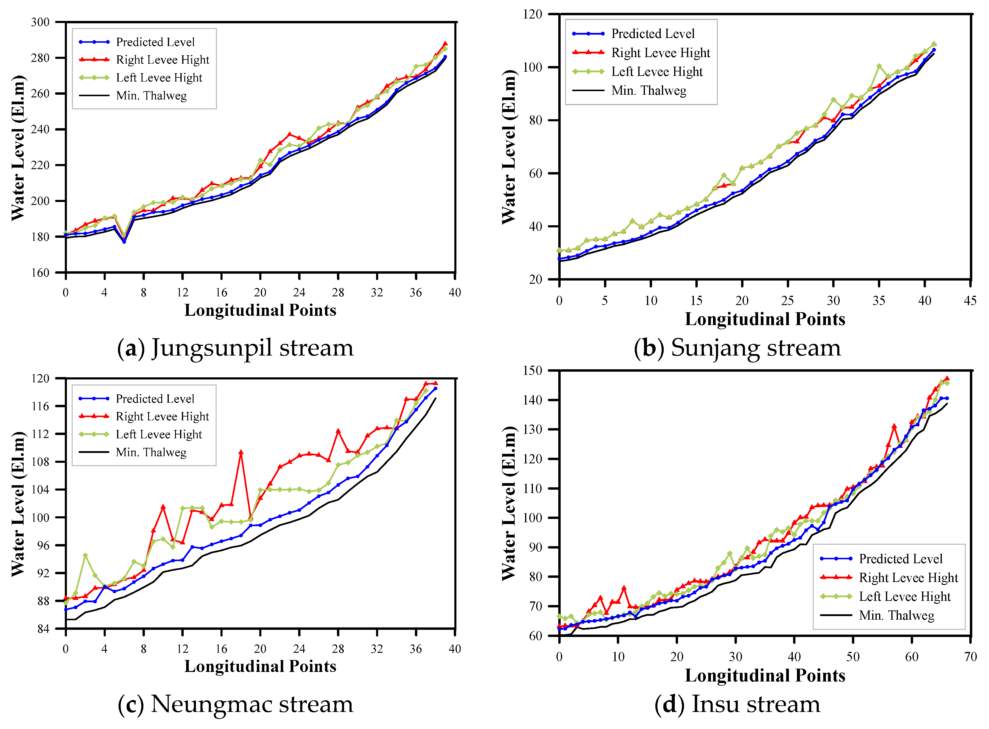
4.3. Applicability Evaluation of Depth Prediction for Unmeasured Cross-Sections

To evaluate the applicability of a newly developed flood water depth prediction method for unmeasured small stream sections, this research predicted flood water depths to assess which sections overflows occurred in through a comparison with the levee heights, as shown in Figure 13. To assess which sections overflows occurred in, this research used the largest flood events that occurred in 2022, on August 9 for the Insu stream and September 5 for the other three small streams. The predicted depth results, similarly to the observed results, showed no overflow areas, indicating that the newly developed flood water depth prediction method was effective for predicting flood water depths in the unmeasured cross-sections of small streams.

5. Conclusions

The increasing frequency of natural disasters due to climate change, along with urbanization and population growth, has raised flood risks. Efforts to reduce these risks require the acquisition of more measurement data and the improvement of early warning technologies based on observed data. Recent studies have shown a global rise in flood damage, with sharp increases recorded in 2020 and 2021. In Korea, over 22,000 small streams with steep slopes and complex flow behaviors present major flood management challenges. Given the severe climate change impacts on small streams, immediate and effective mitigation measures are urgently needed for vulnerable areas.

In response to this, this study developed a flood early warning framework (FEWF) to predict the water depths in unmeasured small stream sections. The framework predicted discharges using nonlinear rainfall–discharge nomographs constructed using historical rainfall data from AWSs and CCTV-based automatic discharge measurements. Rainfall forecasts by the MAPLE were input into the nomographs, which updated in real time using a robust constrained nonlinear optimization algorithm. If the predicted and measured discharge residuals exceeded the thresholds, the nomographs were rebuilt to maintain prediction accuracy. The predicted discharges were then used with the Manning formula to estimate water depths in unmeasured cross-sections.

To improve accuracy, this study developed a nonlinear optimization approach that minimized the presence of progressively increasing residuals. This method showed high accuracy in predicting flood discharges and water depths in unmeasured sections of small streams. The results confirmed the FEWF’s effectiveness in predicting flood discharges and depths using the MAPLE-predicted rainfall. Discharge predictions made one hour before events closely matched observations, with the predictions for the Insu and Sunjang streams showing the best accuracy. The predicted discharge discrepancy ratios followed a normal distribution, confirming minimal bias and strong predictive performance. The water depth predictions based on FEWF outputs also agreed closely with the observed measurements, especially for the Insu and Neungmac streams. Validation against levee heights during 2022’s largest floods confirmed that the model accurately assessed the flood risks without predicting false overflows.

This study emphasized that the FEWF provides highly accurate flood depth predictions, enabling proactive flood management and reducing casualties. It also highlighted the importance of integrating hydrodynamic measurement data into rainfall, discharge, and depth predictions. By delivering rapid and accurate predictions using real-time data, the framework proved effective in reducing flood damage around small streams. The study recommends applying and validating the FEWF across additional small streams to develop a nationwide flood prediction and warning system.

However, the framework’s predictive accuracy is highly dependent on the quality of the input data, particularly real-time rainfall and discharge measurements. If the measured data are sparse, delayed, or inaccurate, the resulting predictions will also be unreliable. Additionally, the reliance on CCTV-based discharge estimation can introduce errors under poor visibility or sensor malfunctions. These limitations highlight the need for continued investment in high-quality monitoring infrastructure and robust error-handling strategies within early warning systems.

References

1. Joint Ministries. 2023 Climate Change Report; KMA: Daejeon, Republic of Korea, 2023. [Google Scholar]
2. UNDRR. Annual Report 2023; United Nations Office for Disaster Risk Reduction: Geneva, Switzerland, 2024. [Google Scholar]
3. MOIS. Natural Disasters Yearbook 2023; MOIS: Sejong, Republic of Korea, 2023. [Google Scholar]
4. Yang, N.; Zhang, L.; Yu, H.; Gao, J.; Zhang, H.; Xu, Y.; Wan, X. Quantifying the Impact of Climate Change and Human Activities on Multiobjective Water Resource Management in the Hanjiang River Basin, China. J. Water Resour. Plan. Manag. 2025, 151, 05025001. [Google Scholar] [CrossRef]
5. Gaál, L.; Szolgay, J.; Kohnová, S.; Parajka, J.; Merz, R.; Viglione, A.; Blöschl, G. Flood timescales: Understanding the interplay of climate and catchment processes through comparative hydrology. Water Resour. Res. 2012, 48, w04511. [Google Scholar] [CrossRef]
6. Gomi, T.; Sidle, R.C.; Richardson, J.S. Understanding processes and downstream linkages of headwater systems: Headwaters differ from downstream reaches by their close coupling to hillslope processes, more temporal and spatial variation, and their need for different means of protection from land use. BioScience 2002, 52, 905–916. [Google Scholar] [CrossRef]
7. Hewlett, J.D. The varying source area of streamflow from upland basins. In Proceedings of the Symposium on Interdisciplinary Aspect of Watershed Management, Bozeman, MT, USA, 3–6 August 1970; ASCE: New York, NK, USA, 1970; pp. 65–83. [Google Scholar]
8. Hunter, M.A.; Quinn, T.; Hayes, M.P. Low flow spatial characteristics in forested headwater channels of southwest Washington. J. Am. Water Resour. Assoc. 2005, 41, 503–516. [Google Scholar] [CrossRef]
9. McGlynn, B.L.; McDonnell, J.J.; Seibert, J.; Kendall, C. Scale effects on headwater catchment runoff timing, flow sources, and groundwater-streamflow relations. Water Resour. Res. 2004, 40, w07504. [Google Scholar] [CrossRef]
10. McNamara, J.P.; Chandler, D.; Seyfried, M.; Achet, S. Soil moisture states, lateral flow, and streamflow generation in a semi-arid, snowmelt-driven catchment. Hydrol. Process. Int. J. 2005, 19, 4023–4038. [Google Scholar] [CrossRef]
11. Whiting, P.J.; Bradley, J.B. A process-based classification system for headwater streams. Earth Surf. Process. Landf. 1993, 18, 603–612. [Google Scholar] [CrossRef]
12. Thomas, D. Field studies of hillslope flow processes. In Hillslope Hydrology; Kirkby, M.J., Ed.; John Wiley & Sons: New York, NK, USA, 1978. [Google Scholar]
13. Woods, R.; Sivapalan, M.; Duncan, M. Investigating the representative elementary area concept: An approach based on field data. Hydrol. Process. 1995, 9, 291–312. [Google Scholar] [CrossRef]
14. Nadeau, T.L.; Rains, M.C. Hydrological connectivity between headwater streams and downstream waters: How science can inform policy 1. JAWRA J. Am. Water Resour. Assoc. 2007, 43, 118–133. [Google Scholar] [CrossRef]
15. Robinson, J.S.; Sivapalan, M.; Snell, J.D. On the relative roles of hillslope processes, channel routing, and network geomorphology in the hydrologic response of natural catchments. Water Resour. Res. 1995, 31, 3089–3101. [Google Scholar] [CrossRef]
16. Pingel, N.; Jones, C.; Ford, D. Estimating forecast lead time. Nat. Hazards Rev. 2005, 6, 60–66. [Google Scholar] [CrossRef]
17. Vieux, B.E. Distributed Hydrologic Modeling Using GIS. In Distributed Hydrologic Modeling Using GIS; Springer: Dordrecht, The Netherlands, 2001; pp. 1–17. [Google Scholar]
18. Cheong, T.; Joo, J.; Byun, H. Advancement of Automatic Discharge Measurement Technology to Enhance Disaster-Safety Codes Forsmall Stream; NDMIPR (ER)-2019-06-01; National Disaster Management Institute: Ulsan, Republic of Korea, 2019. [Google Scholar]
19. Cheong, T.S.; Kim, S.; Koo, K.M. Development of measured hydrodynamic information-based flood early warning system for small streams. Water Res. 2024, 263, 122159. [Google Scholar] [CrossRef]
20. World Meteorological Organization. Manual on Stream Gauging, Vol. I: Fieldwork Vol. II: Computation of Discharge; World Meteorological Organization: Geneva, Switzerland, 2010; Volume WMO-No. 1044. [Google Scholar]
21. ISO Standard No. 9196:1992; Liquid Flow Measurement in Open Channels—Flow Measurements Under Ice Conditions. American National Standards Institute: New York, NK, USA, 1992.
22. Carrigan, P.H. Calibration of US Geological Survey Rainfall-Runoff Model for Peak Flow Synthesis Natural Basins; US Geological Survey: Reston, VA, USA, 1973.
23. Dawdy, D.R.; Lichty, R.W.; Bergmann, J.M. A Rainfall-Runoff Simulation Model for Estimation of Flood Peaks for Small Drainage Basins; US Government Printing Office: Washington, DC, USA, 1972.
24. Lichty, R.W.; Liscum, F. A Rainfall-Runoff Modeling Procedure for Improving Estimates of T-Year (Annual) Floods for Small Drainage Basins; Department of the Interior, Geological Survey: Golden, CO, USA, 1978.
25. Park, H.G.; Choi, H.I.; Jee, H.K. Flood forecasting by using distributed models with ensemble Kalman filter. In Proceedings of the Korea Water Resources Association Conference, Pyeongchang, Republic of Korea, 21 May 2009; pp. 27–31. [Google Scholar]
26. Cheong, T.S.; Choi, C.; Ye, S.J.; Shin, J.; Kim, S.; Koo, K.M. Development of flood early warning frameworks for small streams in Korea. Water 2023, 15, 1808. [Google Scholar] [CrossRef]
27. Bedient, P.B.; Hoblit, B.C.; Gladwell, D.C.; Vieux, B.E. NEXRAD radar for flood prediction in Houston. J. Hydrol. Eng. 2000, 5, 269–277. [Google Scholar] [CrossRef]
28. Bedient, P.B.; Holder, A.; Benavides, J.A.; Vieux, B.E. Radar-based flood warning system applied to tropical storm Allison. J. Hydrol. Eng. 2003, 8, 308–318. [Google Scholar] [CrossRef]
29. Hoblit, B.C.; Vieux, B.E.; Holder, A.W.; Bedient, P.B. Predicting with Precision. Civ. Eng. Mag. (ASCE) 1999, 69, 40–43. [Google Scholar]
30. MSIT. Demonstration of a Standalone Flood Forecasting and Warning System Using AI-Based Flood Prediction Algorithm; Ministry of Science and ICT: Sejong, Republic of Korea, 2019.
31. Casati, B.; Wilson, L.; Stephenson, D.; Nurmi, P.; Ghelli, A.; Pocernich, M.; Damrath, U.; Ebert, E.; Brown, B.; Mason, S. Forecast verification: Current status and future directions. Meteorol. Appl. A J. Forecast. Pract. Appl. Train. Tech. Model. 2008, 15, 3–18. [Google Scholar] [CrossRef]
32. Ebert, E.; McBride, J. Verification of precipitation in weather systems: Determination of systematic errors. J. Hydrol. 2000, 239, 179–202. [Google Scholar] [CrossRef]
33. Lee, J.T.; Seo, K.A.; Hur, S.C. Flood forecasting and warning system using real-time hydrologic observed data from the Jungnang stream basin. J. Korea Water Resour. Assoc. 2010, 43, 51–65. [Google Scholar] [CrossRef]
34. Bae, D.H.; Shim, J.B.; Yoon, S.S. Development and assessment of flow nomograph for the real-time flood forecasting in Cheonggye stream. J. Korea Water Resour. Assoc. 2012, 45, 1107–1119. [Google Scholar] [CrossRef]
35. Jang, C.H.; Kim, H.J. Development of flood runoff characteristics nomograph for small catchment using R-programming. In Proceedings of the Korea Water Resources Association Conference, Goseong, Republic of Korea, 28 May 2015; p. 590. [Google Scholar]
36. USGS. Flood Frequency and Storm Runoff of Urban Areas of Memphis and Shelby County, Tennessee; USGS: Reston, VA, USA, 1984; p. 110.
37. Hill, A.V. The possible effects of the aggregation of the molecules of hemoglobin on its dissociation curves. J. Physiol. 1910, 40, iv–vii. [Google Scholar]
38. Leow, M.K.S. Configuration of the hemoglobin oxygen dissociation curve demystified: A basic mathematical proof for medical and biological sciences undergraduates. Adv. Physiol. Educ. 2007, 31, 198–201. [Google Scholar] [CrossRef] [PubMed]
39. Draper, N.R.; Smith, H. Applied Regression Analysis; John Wiley and Sons: Hoboken, NJ, USA, 1998; Volume 326. [Google Scholar]
40. Gallant. Nonlinear regression. Am. Stat. 1975, 29, 73–81. [Google Scholar] [CrossRef]
41. Hanson, S.J. Confidence intervals for nonlinear regression: A basic program. Behav. Res. Methods Instrum. 1978, 10, 437–441. [Google Scholar] [CrossRef]
42. Huber, P.J.; Elvezio, M.R. Robust Statistics; Wiley: Hoboken, NJ, USA, 2011. [Google Scholar]
43. Holland, P.W.; Welsch, R.E. Robust regression using iteratively reweighted least-squares. Commun. Stat. Theory Methods 1977, 6, 813–827. [Google Scholar] [CrossRef]
44. Alfieri, L.; Zsoter, E.; Harrigan, S.; Hirpa, F.A.; Lavaysse, C.; Prudhomme, C.; Salamon, P. Range-dependent thresholds for global flood early warning. J. Hydrol. X 2019, 4, 100034. [Google Scholar] [CrossRef] [PubMed]
45. Weber de Melo, W.; Iglesias, I.; Pinho, J. Early warning system for floods at estuarine areas: Combining artificial intelligence with process-based models. Nat. Hazards 2024, 121, 4615–4638. [Google Scholar] [CrossRef]
46. Gu, Q.; Chai, F.; Zang, W.; Zhang, H.; Hao, X.; Xu, H. A Two-Level Early Warning System on Urban Floods Caused by Rainstorm. Sustainability 2025, 17, 2147. [Google Scholar] [CrossRef]
47. White, W.R.; Mill, H.; Crabbe, A.D. Sediment Transport: An Appraisal of Available Methods: Volume 1: Summary of Existing Theories: Volume 2: Performance of Theoretical Methods When Applied to Flume and Field Data; Hydraulics Research Station: Wad Madani, Sudan, 1972. [Google Scholar]
Figure 1. Map showing the locations of the small streams and the rainfall gauging stations.
Water 17 01467 g001
Figure 2. Methodological framework for the prediction of the water depth in an unmeasured cross-section of a small stream.
Water 17 01467 g002
Figure 3. Locations of sections where flood water depth was predicted and measured point (MP) in four small streams.
Water 17 01467 g003aWater 17 01467 g003b
Figure 4. Cross-sections of four studied small streams at measurement points.
Water 17 01467 g004
Figure 5. Flowchart of the flood early warning framework for the prediction of the water depth in an unmeasured cross-section of a small stream.
Water 17 01467 g005
Figure 6. Comparison of the rainfall–discharge nomographs developed for each small stream by using the RCNOA.
Water 17 01467 g006
Figure 7. The warning criteria in the small stream FEWF. The time-distributed depth of the Sunjang stream was measured on 29 August 2020.
Water 17 01467 g007
Figure 8. Comparison of MAPLE-predicted and measured rainfall.
Water 17 01467 g008
Figure 9. Comparison of the time–discharge distribution results predicted by using the FEWF with the data measured by using CADMT for four small streams.
Water 17 01467 g009
Figure 10. Comparison of the discrepancy ratio distribution results for the discharge predicted by using the FEWF and the predicted rainfall data for four small streams.
Water 17 01467 g010
Figure 11. Comparison of the time–depth distribution results predicted by using the FEWF with the data measured by using CADMT for four small streams.
Water 17 01467 g011
Figure 12. Comparison of the discrepancy ratio distribution results for the depth predicted by using the FEWF and the predicted discharge in the four small streams tested.
Water 17 01467 g012
Figure 13. Comparisons of water level distribution results predicted by using the FEWF with measured data by using the CADMT for four test small stream.
Water 17 01467 g013