1. Introduction
Urban parks and green spaces have an essential role in improving the urban environment, providing social functionality, offering a number of social benefits in citizens’ quality of life, and becoming an essential part of the landscape in novel urban ecosystems [
1,
2,
3,
4]. It has also been recognized that urban green spaces favor human health [
5,
6,
7,
8]. Forest urban parks contribute to managing urban climate through evapotranspiration processes, cooling air by shading and breezes, mitigating the effects of urban warming in city neighborhoods, and improving thermal comfort [
9,
10,
11,
12,
13]. Furthermore, trees are able to reduce air pollutants [
14]. The ecological reforestation of native trees, understory plants, and meadows in forest parks by human interventions prevents long-term wildlife and biodiversity losses [
15,
16,
17,
18,
19]. The water environment, characterized by ponds, canals, and riverbanks, is also an essential component within the ecosystem services in urban green spaces [
20]. Indeed, parks may have impacts on the regulation of water quality, also preventing water shortage by reducing surface water runoff [
21].
Water bodies, soil, and canal bed sediments in urban parks may experience a variety of anthropogenic inputs, including potentially toxic elements (PTEs) and organic pollutants, primarily depending on the population density [
22,
23] and ongoing urbanization. Major PTE sources in urban settings include vehicle traffic and industrial activities located nearby [
24,
25,
26,
27,
28]; furthermore, the use of pesticides (such as herbicides, insecticides, fungicides) in an urban environment may affect ecological and human health [
29].
The present study focuses on the geochemical characterization (including PTEs and organic pesticides) of water, soil, and bed sediments of canals crossing an urban forest park in coastal Versilia, a densely populated area with a strong touristic vocation in the Tuscany region of Italy. The aim was to investigate the hydrogeochemical dynamics and contamination levels of environmental matrices in order to assess the potential human health risk of urban park soil, specifically in relation to PTEs.
2. Study Area
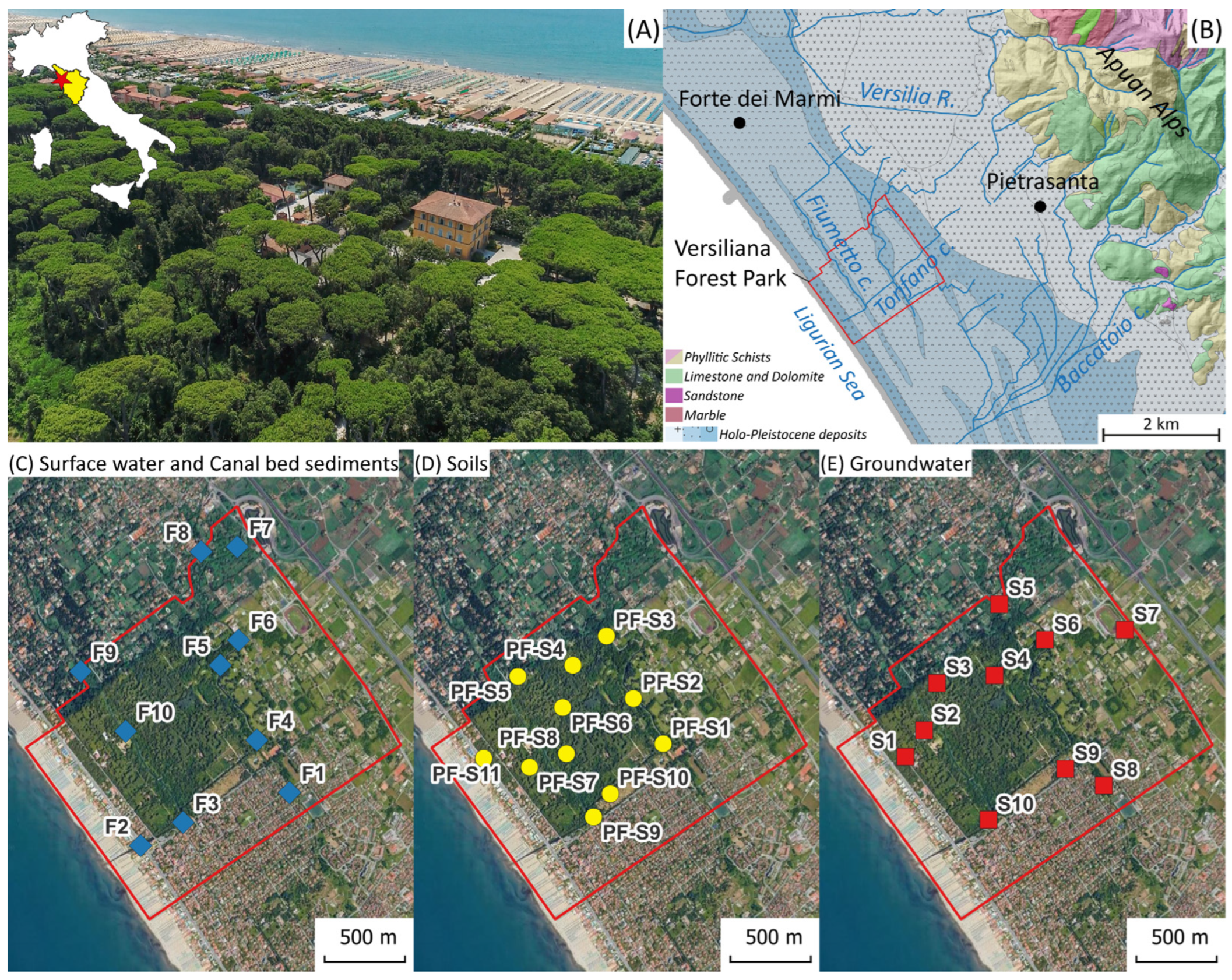
The Versiliana urban park, located along the Versilia coast, Tuscany, Italy (
Figure 1A), extends for about 80 ha and represents an area of recognized environmental value and a forest heritage of historical–cultural and landscape interest. Since 1953, the park has been declared a natural and beautiful landscape of notable public interest, according to Italian legislation. The area, whose vegetation is particularly rich in biodiversity, is highly frequented in the context of sustainable tourism and represents a transit and stopover area for migratory birds.
Versiliana park belongs to the Versilia plain, a 5 km-wide alluvial coastal plain between the Apuan Alps range to the east and the Ligurian Sea to the west (
Figure 1B). The Apuan Alps represent one of the rainiest areas in Italy, reaching a mean annual precipitation of about 3000 mm [
30,
31]. The main watercourses in the Versilia plain originate from the adjacent reliefs, and do not always follow their natural course due to the intense urbanization of the area. The plain is characterized by a number of artificial and drainage canals, associated with past hydraulic reclamation works. From a geological point of view, the Versilia plain is part of a large tectonic basin [
32], filled by continental, transitional, and marine sediments forming a stratigraphic sequence about 2000 m thick, composed of alternate sands, silt, clays, and gravels. Locally, peat layers occur at different depths as discrete stratigraphic levels. Alluvial fan deposits outcrop in the foothills, whereas marine and eolian deposits can be found in the coastal area. The constant supply of sediments from the major watercourses significantly advanced the coastline towards the southwest, producing a regular succession of dunes and depressed marshy areas [
33]. In this context, two main canals, Tonfano and Fiumetto, cross the park, forming small wetlands. The hydrogeological context is characterized by an extended unconfined aquifer, with the water table near the topographic surface. The proximity to the sea makes the aquifer vulnerable to seawater intrusion. A movable mechanical floodgate prevents seawater intrusion into the canals by tidal dynamics and storm surges. Dewatering pumps drain freshwater when the floodgate is closed and act to retain surface water feeding the unconfined aquifer.
3. Materials and Methods
3.1. Sampling
Water, sediment, and soil sampling sites are reported in
Figure 1. Surface water from Fiumetto and Tonfano canals was collected at 10 stations (
Figure 1C) during four different surveys over two years (survey I: 22 May 2023; survey II: 26 September, survey III: 2023; 9 April 2024; survey IV: 18 September 2024) in order to investigate the hydrogeochemical dynamics across seasons, with the aim of identifying emerging issues for management purposes (samples WF1 to WF10 labeled as I, II, III, IV in
Table S1). It must be noted that station WF1 is located on the southern extension of the Tonfano canal, outside the Versiliana green space, and directly receives urban runoff. A pressure-vacuum lysimeter was used to collect the hyporheic zone porewater at about a 20 cm depth in bed sediments from the WF2 station in the Fiumetto canal (sample F2-lys). A representative water sample from the Versilia River, largely contributing to feeding the Versiliana canal network, was also collected (sample F-ver). Groundwater (
Figure 1E) was collected at a shallower flow zone depth (less than 5 m) during a single survey (22 May 2023) through 10 depth-integrated piezometers of 10 and 30 m depth (10 m depth: samples S1, S3, S4, S5, S7, S8, S9, S10; 30 m depth: sample S2, S6) by using a bailer. Water samples were filtered through a 0.45 μm membrane filter in the field, stored in pre-cleaned polyethylene bottles, and kept refrigerated until laboratory analysis. Ultrapure nitric acid was used as a preservative. The amount of rainfall during the sampling period was measured by the Pietrasanta rain gauge, located 5 k from the study area. The morphology of the piezometric surface was obtained from the piezometers and superficial water measurements through monthly surveys of the water level (from May to December 2023) in order to investigate the hydrodynamic behavior of the Versiliana unconfined aquifer and the influence of rainfall.
In order to evaluate the effects of the catchment depositional dynamics on bulk chemistry, canal bed sediments were collected using a Van Veen grab sampler during four surveys at the same time and location as the surface water (
Figure 1C; samples SF1 to SF10 labelled I, II, III, IV, except station 9, which was not sampled for sediments). Soil samples were collected at 11 stations (
Figure 1D) during a single survey (May 2023; samples PF-S1 to PF-S11), with the aim of representing the Versiliana geographical space. Due to the lack of known contamination sources and geochemical variability, the soil sampling strategy followed a non-aligned grid design and equally spaced cells. In each cell, the sampling site was placed considering both auxiliary data, such as road proximity and open fields or throughfall inputs under tree crowns, or randomly. Composite soil samples were taken at 5–20 cm depth by using a hand auger. Sediment and soil samples were stored in plastic bags, dried at room temperature under laminar flow until constant weight, homogenized, quartered, and dry-sieved to less than 2 mm.
Peat layers a few decimeters thick were collected from the continuous drilling cores at stations S4, S9, and S10.
3.2. Water Analysis
Temperature (°C), electrical conductivity (EC, μS/cm at 25 °C), pH, and dissolved oxygen (DO) were measured in the field by using Delta OHM HD 2105.1 and 2109.1 instruments (Caselle di Selvazzano, Italy), respectively, taking readings as soon as meters stabilized. Uncertainties were ±0.8 °C, ±0.5% μS/cm, ±0.02 pH unit, and ±0.2 mg/L. Alkalinity, totally assigned to bicarbonate, was measured by acidimetric titration using 0.1 N HCl. Major ions were determined by ion-chromatography using a Thermo Fisher Scientific ICS-900 instrument (Waltham, MA, USA). Relative standard deviation (RSD) was within 5%. Trace element concentrations were determined by ICP-MS using an Agilent 7850 (Santa Clara, CA, USA). The EnviroMAT ES-L and EU-L reference waters were analyzed together with samples. Precision (10 replicates) was better than 5% RSD except for Be, Fe, Zn, and Pb (5–10%). Deviations from the certified standard values (10 replicates) were less than 5%, except for As and Pb. A submersible CTD-diver (van Essen Instruments, Deft, The Netherlands) was used in each piezometer to record the EC-depth profile (accuracy ±1% of reading) in order to evaluate the seawater-flow pathway inside the aquifer.
3.3. Sediment, Soil, and Peat Analysis
Sediment, soil, and peat samples were digested by using the Ethos Easy microwave platform (Milestone Srl, Sorisole, Italy) (US EPA Method 3052, reversed aqua regia). Trace elements, including PTEs, were determined by ICP-MS using an Agilent 7850. The analytical uncertainty was evaluated by repeated analysis of reference material ERM-CC018. RSD was below 5% except for As (6%) and Co (8%).
For organic pesticide analysis, sediment samples were dried overnight at room temperature in clean room. About 2 or 3 g of sediment was placed in a ceramic crucible in an oven to dry overnight, at about 110 °C, to have an estimate of the dry weight. Sediment samples were pulverized by grinding in a mortar; an aliquot of 3 g was placed in a 50 mL vial equipped with an aluminum crimp cap, and 10 mL of hexane: acetone (1:1) was added. Samples were subjected to ultrasonication for 15 min at room temperature and then centrifuged for 2 min at 3000 rpm; the supernatant was recovered. The ultrasonication and centrifuge cycle was repeated two times with the addition of 5 mL of solvent per cycle; once the supernatant was recovered, the volume was reduced to 2 mL using a centrifugal evaporator. A solvent change was carried out by adding 2 mL of isooctane, and the volume was reduced to 1 mL. The analyses were carried out with a gas chromatograph coupled to a tandem mass spectrometer (Agilent GC 7890–MS 7010, Santa Clara, CA, USA) equipped with an HP-5MS UI capillary column (30 m, i.d. 0.25 mm, 0.25 μm, 5% phenyl 95% methylpolysiloxane). Pesticide mixtures (Custom Pesticide Mix and EPA 8080 Pesticides) were used to construct calibration curves. Certified reference material CRM818 was used to determine the extraction yield and to verify the robustness of the procedure. The analytes were identified with the software “Agilent MassHunter Qualitative Analysis” (version B.0701, Agilent Technologies) by comparing the mass spectra with those available in a NIST library present in the software “NIST MS Search” and quantified with the software “Agilent MassHunter Quantitative Analysis” (version B.0701, Agilent Technologies).
3.4. Leaching Test and Risk Assessment
In order to evaluate contaminant migration from soil to groundwater, the leachate analytical ASTM model was applied [
34]. The model accounts for dissolution of contaminants into infiltrating water, assuming equilibrium partitioning and uniform dilution within the underlying unconfined aquifer. A similar steady-state analytical model is suggested by risk assessment USEPA guidelines [
35,
36]. The estimated dissolved concentration (
Cgw, mg/L) is obtained from the concentration in soil (
Csoil, mg/kg) according to:
where
Kws (L/kg) is the linear equilibrium partitioning coefficient for a given contaminant, given by:
where
ρs is the soil bulk density,
θw is the water-filled soil porosity,
θa is the air-filled soil porosity,
Kd is the distribution coefficient, and
H is Henry’s law constant. The
LDF (leachate dilution factor) accounts for dilution occurring when the contaminant is transferred from the leachate to groundwater:
where
δgw is the groundwater mixing zone height,
Vgw is the groundwater Darcy velocity,
W is the width of the source-zone area longitudinal to the groundwater flow, and
Ief is the rainwater infiltration rate (capping systems are considered absent). The site-specific or recommended values are reported in
Table S2. These analytical models have been applied to back-calculate screening levels in soil (SSLs) for groundwater protection, to be compared with regulatory concentration thresholds. Exposure equations and pathway models for a recreational scenario were also run in reverse to calculate the SSL intended to be protective for human health (corresponding to a 10
−6 risk level for carcinogens and a hazard index of 1 for non-carcinogens), applying a deterministic approach [
34,
35,
36,
37,
38] combining exposure assumptions and toxicity data. The Risk-net software (version 3.1.1pro, September 2019,
http://www.reconnet.net/Software.htm (accessed on 15 March 2025)) was used.
4. Results
4.1. Analysis of Piezometric Data
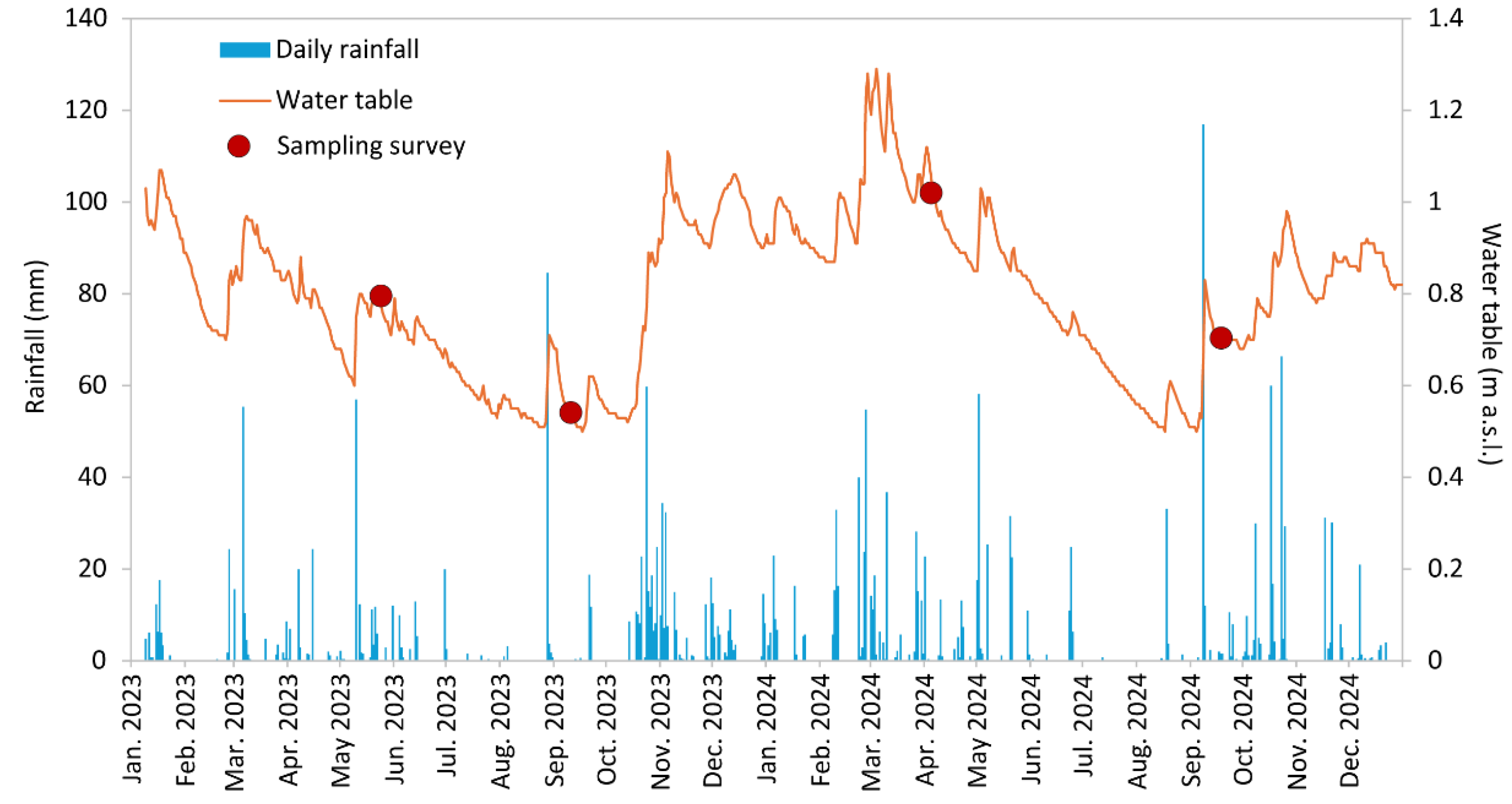
The groundwater hydrograph, representing the changes in water table depth over time and rainfall during two-year surveys (2023–2024), is shown in
Figure 2. The rainfall–recharge relationship is a complex function of rainfall infiltration and canal flow, and even if the recharge potential for the unconfined aquifer by rainwater has not been quantified, a water table rise in the rainy season is clearly observed. Moreover, the water table response time to rainfall appears to be rapid (within hours).
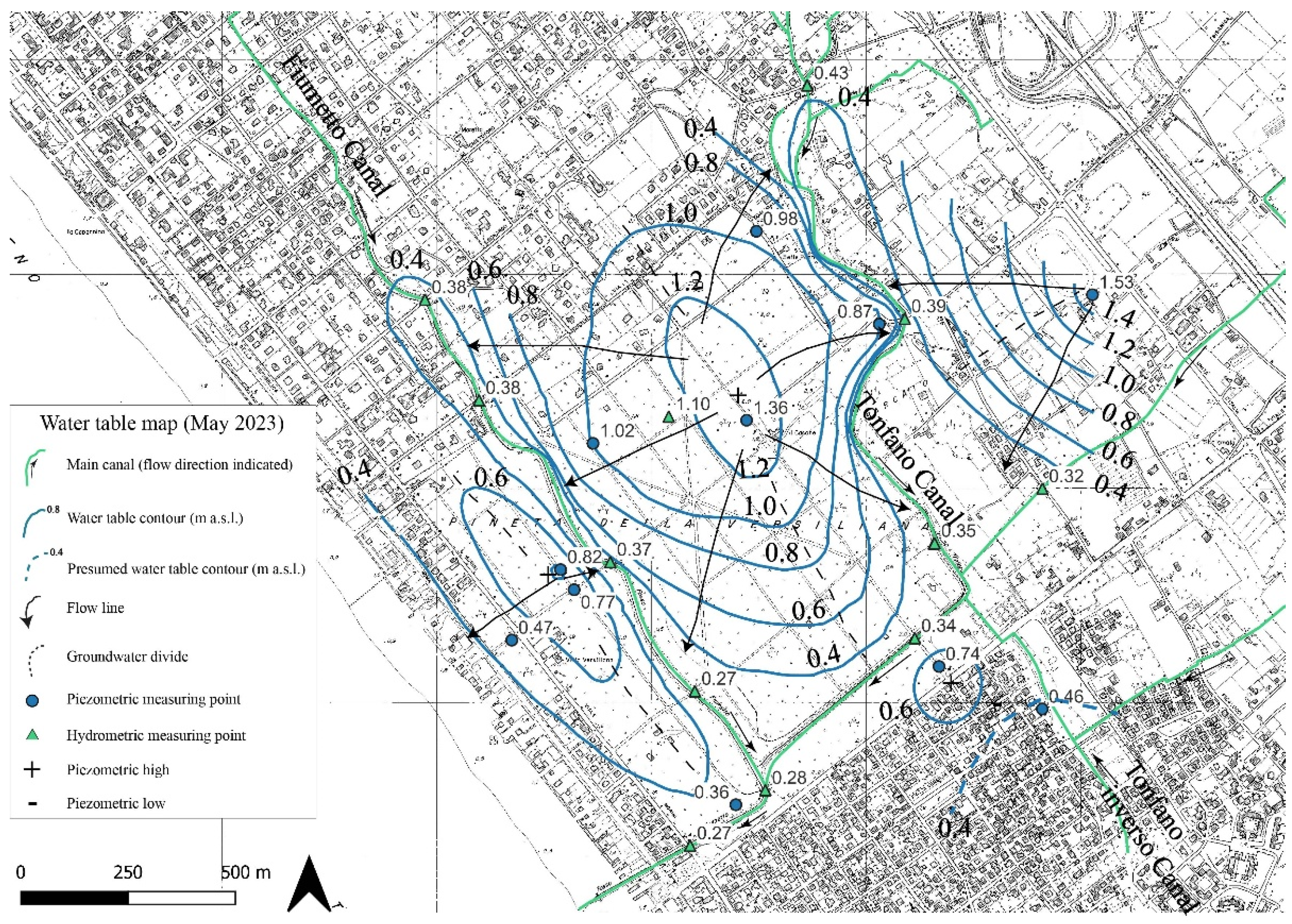
The piezometric surface was obtained by interpolating the water table depth time series. Although fluctuations were observed depending on the rainfall regime, flow directions did not change significantly during the different surveys, and a single water table map, intended as representative (May 2023), is shown (
Figure 3). It can be observed that three piezometric domes are present, which are aligned along the sand-dune system that characterizes the area. The Fiumetto and Tonfano canals mostly act as groundwater drainage canals, even though infiltration from canals may recharge the aquifer during the dry season.
Electrical conductivity in the groundwater samples ranged between 673 and 2370 µS/cm and between 787 and 6950 µS/cm in shallow and deeper piezometers, respectively, reflecting a saline water contribution. No-flushing continuous EC vertical profiles (
Figure 4) provide baseline data to identify seawater intrusion, highlighting complex spatial patterns. It has to be noted that the S10 piezometer (10 m deep) was particularly stressed (EC more than 20,000 µS/cm) and that salinity sharply increased from a shallow depth in the S2 piezometer (30 m deep).
4.2. Water Chemistry
The physico-chemical parameters and major ion concentration for groundwater, surface water, and hyporheic zone pore water are reported in
Table S1.
The temperature in groundwater ranged between 14.6 and 17.1 °C. In canal water, the temperature during the different surveys varied from 14.1 to 21.8 °C (average temperature: 17.2, 19.3, 15.3, and 18.9 °C in surveys I to IV, respectively). The temperature of pore water was 19 °C. The temperature of the Versilia River water, collected in February 2023, was 9 °C. The pH in groundwater and canal water ranged between 7.2 and 7.7 and between 7.2 and 7.8, respectively; no significant pH changes were observed during the different surveys. The pH of pore water was 7.2. The measured pH is consistent with equilibria of dissolved carbonate, ubiquitous in the aquifer and canal sediments, and with pCO2 in the range of 10–1.8 and 10–2.5 atm. Water from the Versilia River (sample F-ver) was distinguished by its more alkaline signature (pH = 8.3), consistent with carbonate equilibrium under atmospheric CO2 in an open system.
Electrical conductivity in canal water ranged between 351 and 723 µS/cm, 349 and 1716 µS/cm, 411 and 1058 µS/cm, and 378 and 1284 µS/cm in surveys I, II, III, and IV, respectively. The highest values were measured during survey II, in particular, in samples WF1, WF2, and WF3 from the southern segment of Tonfano canal, and in samples WF9 and WF10 towards the shoreline. The Versilia River was characterized by freshwater (EC = 195 µS/cm), consistent with a major supply from the Apuan Alps karst hydrosystem. The dissolved oxygen measured in canal water during survey II (DO in the range between 2.8 and 6.8 mg/L) and in pore water (DO = 0.7 mg/L) indicates that the original air-saturated oxygen content was modified at different scales through chemical and/or biological processes.
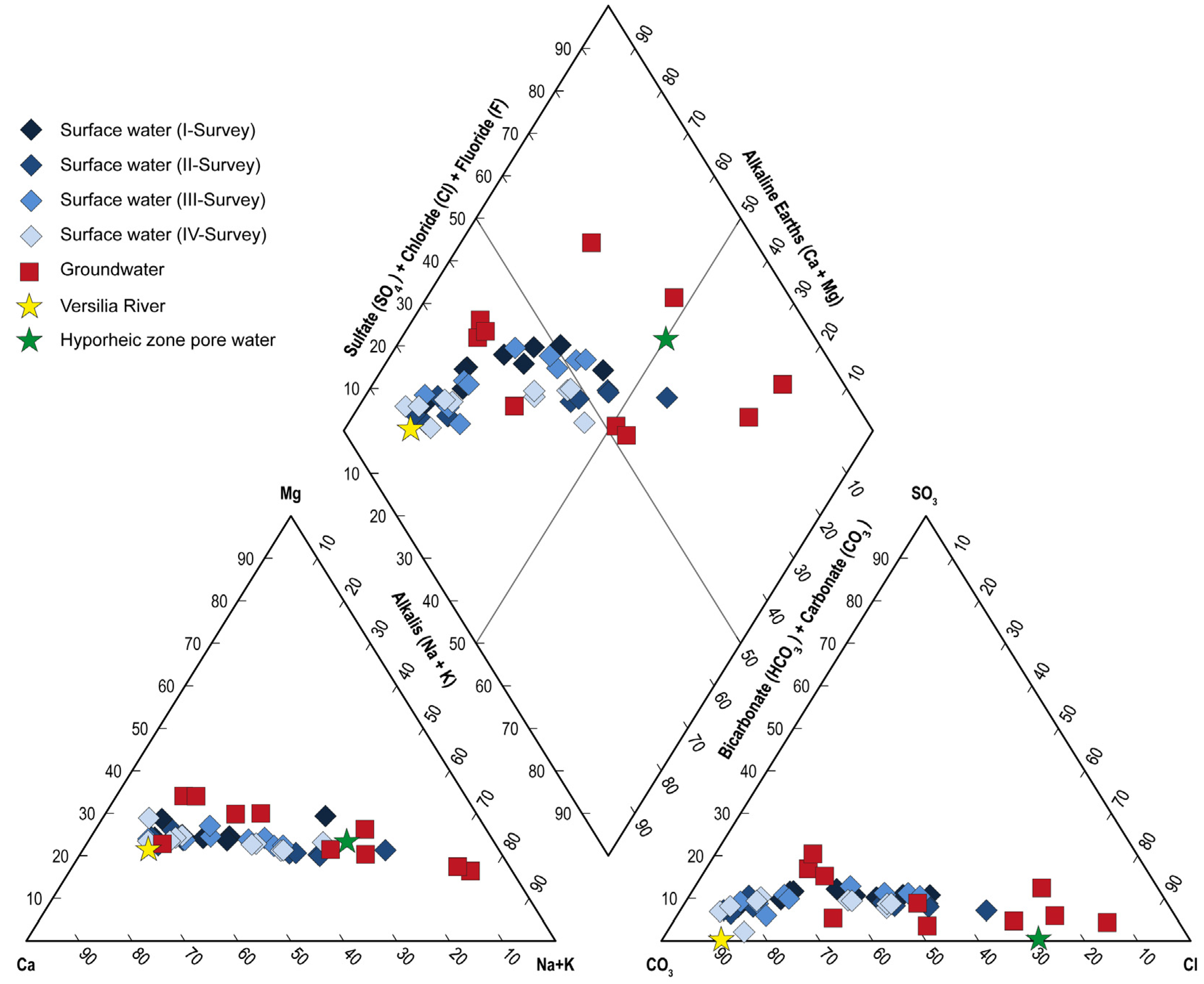
The major ion chemistry of groundwater and the temporal pattern for canal water is shown in the Piper diagram (
Figure 5).
Water-type classification using speciation results (Geochemist’s Workbench
® software, release 12) indicates that groundwater ranged from the Ca-HCO
3 water type (samples S6, S7, S8, S9) to the NaCl (samples S1, S2, S5, S10), CaCl
2, and Na-HCO
3 water types (samples S3 and S4), revealing the combined effects of mixing and cation exchange processes when seawater intrudes into the coastal freshwater aquifer. However, the distribution in the diagram indicates that other reactions may take place besides cation exchange. In particular, the variable deficit in the sulfate content observed in some samples (S1, S2, S3, S10) compared with conservative mixing indicates sulfate reduction in anoxic environments; the sulfate excess (in particular, S6, S7, S8) highlights the potential role of sulfide stability in the aquifer. Water from the Versilia River belonged to the Ca-HCO
3 type. Most waters from canals belonged to the Ca-HCO
3 hydrofacies; a shift towards NaCl (samples WF1, WF2, WF10) and Na-HCO
3 (samples WF3, WF9) was observed in particular during the second survey. Salinization gradually disappeared during the third and fourth surveys, towards the Ca-HCO
3 water type. The occurrence of a freshwater–saltwater mixing zone and possible exchanges of freshwater with leachable sea salts deposed on soil is also highlighted by the Na–Cl correlation diagram (
Figure S1).
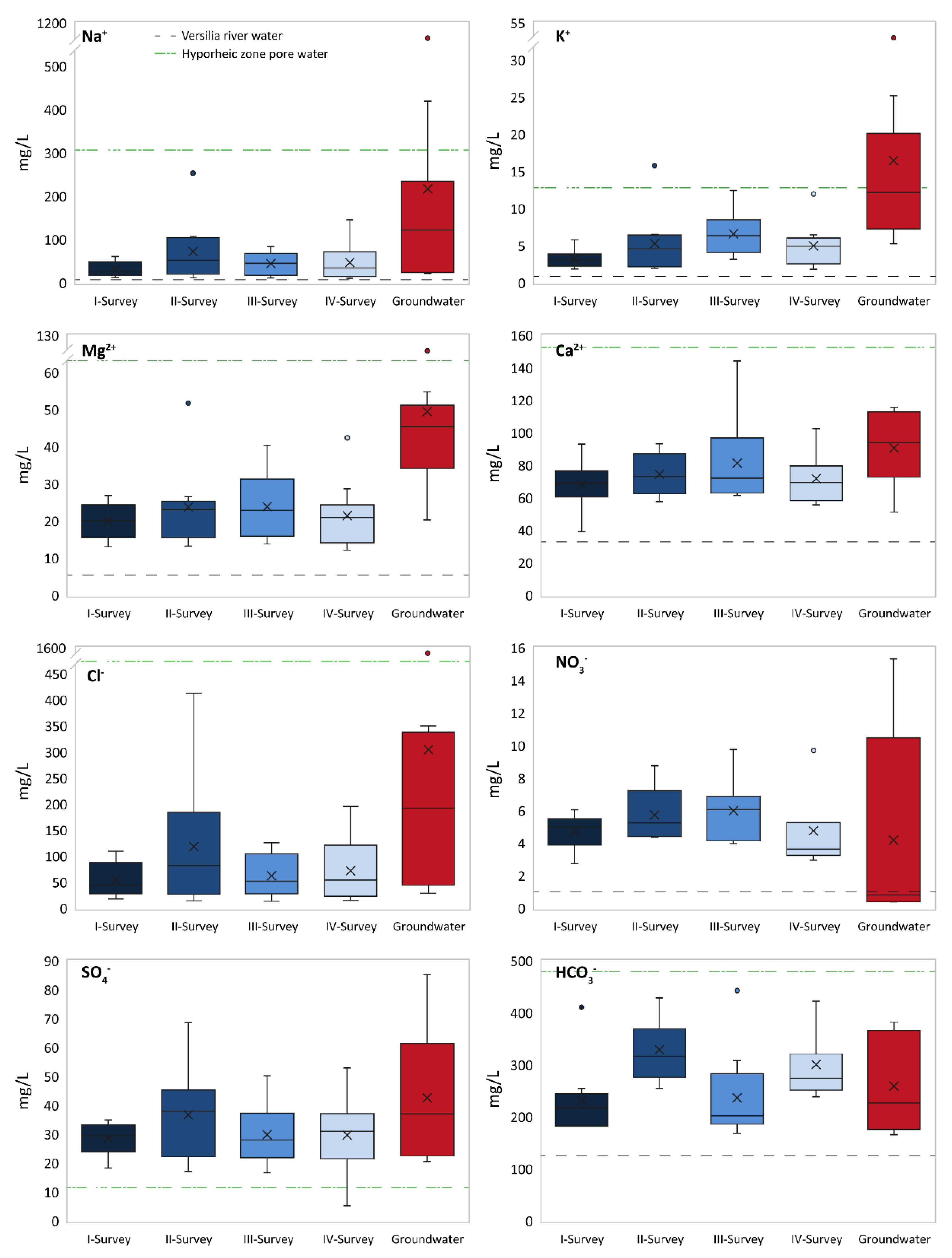
It should be noted that pore water collected within the hyporheic zone belonged to the NaCl type. Considering that canals cannot act as pathways for marine intrusion, the observed salinity might reflect saline groundwater rising and reaching ground level during recharge events. The seasonal variations in the major ion chemistry of canal water, compared with groundwater and the Versilia River, are shown by box plots in
Figure 6. It can be observed that surface water was characterized by a lower concentration for most ions compared with groundwater. Furthermore, canal water showed variable solute inputs compared with Versilia River freshwater; in particular, Na
+, Cl
−, HCO
3−, SO
42−, and K
+ relative enrichments were observed during the second and third surveys, respectively. The pore water from the hyporheic zone showed higher ion concentration except for the low SO
42− content, likely reflecting sulfate reduction.
The trace element concentration measured in the water samples is reported in
Table S1 and graphically shown in the box plots of
Figure 7 for As, Ni, Cu, and Mn.
For most PTEs, the concentration in groundwater and canal water was lower than the thresholds established for water quality by Italian regulations and, in some case, even below the detection limit. Exceptions are arsenic, exceeding the legal limit of 10 µg/L in groundwater (samples S1 and S4) and in canal water (sample WF1–II); manganese, largely exceeding the 50 µg/L threshold in most samples; and iron, exceeding 200 µg/L in groundwater samples S1, S2, S4, and S8.
4.3. Soil, Sediment, and Peat Trace Elements
Soil is represented by alluvial soil, with a shallow water table and organic matter accumulation (eutric gleysols, fluvisols, and cambisols). Trace element data measured in soil are reported in
Table S3. The PTE concentration in most samples was below the limit reported by Italian regulations for soil in recreational settings, even though arsenic showed a concentration of concern in samples PF-S1 to PF-S4; the only exception is sample PF-S4, where Zn, Sb, and Pb largely exceeded the regulatory thresholds.
The trace element concentration in canal bed sediments in the different surveys is reported in
Table S4. The ecotoxicity of contaminants in sediments was evaluated by comparison with the TEC (threshold effect concentration) and PEC (probable effect concentration) quotients [
39]. In particular, TEC indicates the concentration threshold below which no toxic effects to freshwater sediment-dwelling organisms are expected, while harmful effects are expected for concentrations above PEC. The TEC–PEC values for Ni, Cu, Zn, Cd, Pb, Cr, and As are reported in
Table S4. It was observed that Ni exceeded the PEC threshold in all samples; Cr exceeded PEC in samples SF6-I, SF8-I, SF8-II, F8-III, and F8-IV; and As in samples SF1-I, SF2-I, SF1-II, SF1-III, and SF1-IV also revealed an exceedance of TEC values in most samples, and in some cases for Zn, Pb, Cu, and Cd. Moreover, all sediment samples exceeded the quality criteria imposed by the Italian regulation for Ni (threshold of 30 mg/kg) and in some cases for Pb (threshold of 30 mg/kg). Station S7, in particular, showed the highest Ba, Pb, Sb, and Cd concentrations, besides Cu and Zn, in all the surveys. Even though Ba and Sb are currently not included in the sediment quality guidelines, it is worth noting that Sb, which reached 11.1 mg/kg in SF7-IV, is listed as a primary contaminant by the European Union and the U.S. Environmental Protection Agency.
Peat samples were analyzed for arsenic content, considering the tendency of As to accumulate in the peat-rich layers. Arsenic showed a wide range of concentration values in peat collected at different depths. In particular, in the drill cores S4, S9, and S10 (at two different depths), the As content was 51, 32, 7.1, and 336 mg/kg, respectively.
The concentration of organic pesticides in sediments is reported in
Table S5. A number of Sediment Quality Guidelines have been reported for organics in order to estimate sediment pollution (e.g., [
40]). The DDT, DDE, and DDD concentrations, intended as the sum of isomer concentrations of p,p′-DDT and o,p′-DDT, p,p′-DDE and o,p′-DDE, and p,p′-DDD and o,p′-DDD, respectively, exceeded the Canadian freshwater surficial sediment quality guidelines [
41] (SQGs; 1.19, 1.42, and 3.54 ng/g, respectively) for DDT in most samples, in particular during surveys I and II and for DDE during survey IV, and the probable effect levels (PELs; 4.77, 6.76, and 8.51 ng/g, respectively) for DDT in samples SF7-I, SF8-I, SF10-II, and SF10-III and for DDD in samples SF7-III, SF10-III, SF3-IV, and SF10-IV. Most sediments also exceeded the EPA 1.6 ng/g selected benchmark value for DDT under the Comprehensive Environmental Response, Compensation and Liability Act [
42]. The same samples also exceeded the Australian recommended toxicant default guideline values for sediment quality for DDT and DDD (1.2 and 3.5 ng/g, respectively), and were below the threshold for DDE (1.4 ng/g). Sediments collected at stations SF8 and SF10 were the most contaminated. The ΣHCH pesticide concentration ranged between 0.003 ng/g and 0.279 ng/g; the only exception was sample SF2-II, with the highest concentration (8.96 ng/g), exceeding the CCME value (0.99 ng/g).
The heptachlor epoxide content exceeded the CCME-SQG threshold (0.6 ng/g) in most samples, and the CCME-PEL threshold (2.74 ng/g) in survey I (SF2-I, SF3-I, SF8-I) and mostly in survey II (SF1-II, SF2-II, SF3-II, SF4-II, SF8-II, SF10-II), reaching the highest concentration at station SF3. Chlordane exceeded the CCME-PEL value (8.87 ng/g) in samples SF2-II, SF3-II, and SF10-II, reaching the highest concentration (41.02 ng/g) in the latter. Endrin exceeded the CCME-SQG value (2.67 ng/g) in samples SF1-II and SF2-II. In general, the Σ(aldrin, isodrin, heptachlor, heptachlor epoxide, endrin, dieldrin, chlordane, endosulfan, endosulfan sulfate) was highest in sediments from survey II, in particular at sampling stations SF1, SF2, SF3, and SF10 (40.92, 27.86, 42.26, and 49.12 ng/g, respectively). Organohalogens Σ(trifluoralin, benfluoralin, fludioxonil, alachlor, metolachlor, and vinclozolin) showed the highest content in the sediments collected during survey II, in particular in samples SF1-II and SF4-II (13.53 and 18.56 ng/g, respectively). The highest content of non-chlorinated thiophosphates was measured during survey II, in particular, in sample SF1-II [Σ(malathion, fenthion, ethion): 256.2 ng/g]. Also, the concentration of metalaxyl fungicide was the highest in sediments collected during survey II, reaching 263, 468, 453, and 297 ng/g in samples SF1-II, SF2-II, SF3-II, and SF4-II, respectively.
4.4. Risk-Based Arsenic Leaching and Soil Screening Level
Arsenic in soil may lead to a long-term risk to groundwater, since As may be gradually leached by infiltrating water. The calculated groundwater concentration for arsenic, as expected by applying the leachate ASTM model and the average soil concentration (7.9 mg/kg) and the site-specific experimental
Kd (1808 L/kg), yielded a CGW value of 4.27 µg/L. The corresponding SSL for the protection of groundwater, calculated on the basis of the experimental
Kd, was 18.5 mg/kg, close to the threshold value imposed by Italian regulations (20 mg/kg). The calculated arsenic SSL (
Table 1), considering a recreational outdoor setting, for each exposure pathway and carcinogenic effects, was 2.86 mg/kg, lower than the concentration threshold in soil reported by Italian regulations. On the contrary, the SSL for non-carcinogenic effects was 1.60 × 10
2 (children) and 1.42 × 10
3 (adults), much higher compared with regulation limits and the maximum As concentration measured in soil.
5. Discussion
Canal bed sediments and soil represent an important sink for PTEs and organic pollutants in urban parks, related to both watershed background inputs and more localized anthropogenic sources of pollution, such as the emissions in proximity to road traffic, the indiscriminate use of pesticides and fertilizers in urban agriculture, and the effects of nearby industrial areas [
45].
The screening obtained by comparing the measured PTEs concentrations in canal bed sediments with the recommended Sediment Quality Guidelines (SQGs: TEC and PEC values) and Italian regulations indicate concentrations of concern, in particular, for Ni, Cr, As, Zn, Pb, and Cd, in addition to highlighting high Sb and Ba content in one of the sampling stations.
The principal component analysis (PCA; performed using Past 5.3 software [
46]) can be used for contaminant source attribution. The results for canal bed sediments show that the majority of samples clustered in the lower-left quadrant of the PCA plot (
Figure 8). The weak association with organic pollutants indicates a predominantly geogenic origin for PTEs for most samples. In particular, the positive Cr–Ni correlation (R
2 = 0.73) is interpreted as the geochemical fingerprint of ophiolite inheritance, exhibiting naturally high Cr and Ni values. Although not outcropping in the Versilia River catchment, ophiolites representing the reworking of Ligurian ultramafic successions occur in the sedimentary cover of the coastal plain in the area of interest.
The Tl–Sb–Pb–Zn–As inter-element correlations (Tl–Sb: R
2 = 0.86; Zn–Pb: R
2 = 0.81; V–Be: R
2 = 0.91) are attributable to sources from the main orebodies hosted within the Apuan unit [
47]. In particular, the data are consistent with the products of weathered and eroded metalliferous mineralization that characterize the upstream Versilia River basin, as occurring at the dismissed Buca della Vena mine site. The complex mineralization includes V–Sb minerals, Fe–Ti–Sb oxides, and a variety of sulfates and Tl–Hg–As–Sb–(Cu)–Pb sulfosalts [
48]. Arsenic does not show any good correlation when all sediment samples are considered. However, if the samples collected at the SF1 station during the different surveys and at the SF2 and SF3 stations during the first survey, characterized by exceedingly high As content, are excluded, positive linear correlations are obtained (As–Zn: R
2 = 0.91; As–Tl: R
2 = 0.83; As–Pb: R
2 = 0.78). The As excess, in particular, at station SF1, might reflect anthropogenic inputs. This hypothesis is supported by PCA, which shows that the arsenic vector lies between the PTE group and the organic pollutants, implying a mixed origin (
Figure 8). This intermediate positioning thus indicates both geogenic contributions from local lithology and anthropogenic enrichment due to the historical use of arsenic-based pesticides. PCA clearly distinguishes site SF7, placing it along PC1 in association with high concentrations of some PTEs (mainly Ba, Pb, Cd, Sb, Zn, and Cu). This chemical fingerprint likely reflects sources from non-exhaust vehicular emissions [
49,
50,
51], consistent with the site’s proximity to a major road and a motorway exit (toll booth). Furthermore, the high Ba content possibly reflects input from a nearby ceramic factory, where barium carbonate is commonly used [
52]. PCA separates several samples from the second survey campaign (survey II), which are oriented along PC2, showing stronger correlations with organic contaminants, including DDTs, HCB, aldrin, and organophosphates. This suggests a temporary increase in pesticide-related inputs, potentially linked to agricultural/silvicultural activities or surface runoff events.
The areal distribution of As and other PTEs (Pb, Zn, Sb) in canal sediments and soil, formed by sediment parent material deposited by fluvial systems, is shown in
Figure 9.
In order to assess the state of soil contamination, the geoaccumulation index (I
geo) [
53,
54] was calculated (
Table S6 and Figure S2). Considering the difficulty in defining a basin-specific geochemical background, the average composition of upper continental crust as an artificial reference was used [
55]. The results indicate that sample PF-S4 was extremely contaminated for Zn, Sb, and Pb, likely representing a hot spot of mine tailings or smelting slags buried under vegetation cover. This site requires restoration; the contaminated soil should be urgently removed to a landfill, where the pollutants can be managed. As far as arsenic, Pb, and Sb are concerned, all the other soil samples ranged from uncontaminated to moderately contaminated; in particular, arsenic in soil may form highly persistent compounds, and the highest As content was observed in the soil near the side slopes of the easternmost Tonfano canal profile. Furthermore, the soil was moderately to strongly contaminated for selenium (
Figure S2).
Sediments and soil can be regarded both as sinks and as secondary sources for contaminant release to water. The highest As concentration in canal water during the different surveys was observed at station WF1, reaching 19.7 µg/L in WF1-II, a station characterized by the highest arsenic content in sediments. A rough positive correlation (R
2 = 0.67) was observed between As and Mn in canal water collected during the different surveys, if sample WF1-II, with exceedingly low Mn concentration, is excluded from the fitting (
Figure S3). The Mn–As correlation suggests that the reductive dissolution of As-bearing Mn oxides in canal bed sediments might be responsible for the arsenic release to water.
Indeed, a high Mn content characterizes the hyporheic zone pore water under reducing conditions (
Figure S3), indicating that sediments represent manganese-containing environmental systems at Versiliana. Manganese (III/IV) oxides, which form under different environmental conditions, promote oxidation of As(III) in the aqueous phase to the less mobile arsenate As(V) at circum-neutral pH [
56,
57], and both As species can adsorb onto the Mn-oxide mineral surface [
58], forming inner sphere bonds [
59]. The data hence indicate that Mn oxides in sediments might affect the dynamic behavior of As released from soil and mobilization to canal water, possibly contributing to groundwater As contamination through canal–aquifer interactions. Arsenic in soil may also be leached to groundwater, as suggested by applying the ASTM model.
In addition, the mineralized components accumulated within the Versiliana aquifer likely contribute to the As release to groundwater, reaching concentrations exceeding regulatory limits. In particular, the oxidative dissolution of relatively small amounts of As-bearing sulfide minerals distributed in the aquifer may cause a significant As release and represent a possible pathway for As mobilization. Furthermore, the high As concentration measured in peat suggests that As may be sequestered by the natural organic matter deposits that characterize the Versiliana aquifer: spatio-temporal variations of the redox conditions, peat decomposition, and competitive desorption processes may govern As release from peats, acting as a secondary As source in the aquifer. Under water-table rise, the contaminated groundwater discharges into the Versiliana canals, allowing As to be exchanged from groundwater to the surface.
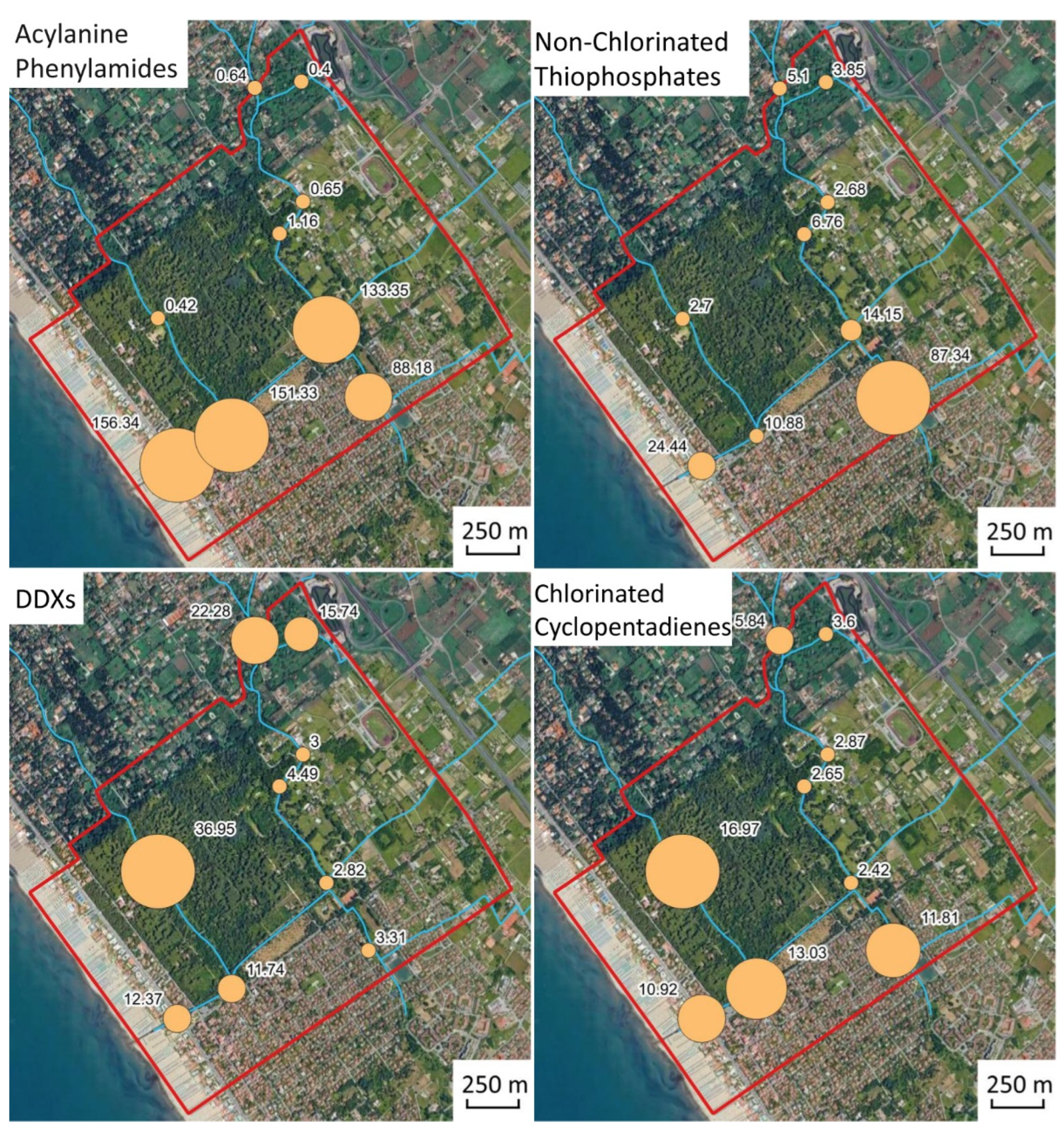
The spatial distribution of pesticide classes is shown in
Figure 10.
The data highlights the legacy of the historical use of organic pesticides in Versiliana park, and their persistence due to the tendency to absorb onto particulate organic matter and to settle in bed sediments [
60]. Indeed, organic pesticides in sediments may be accumulated by benthic organisms, with associated ecological risk. It is worth noting that sediments collected at station SF1 during survey II had the highest malathion as well as high metalaxyl content; high concentration values also characterized samples SF2, SF3, and SF4. In particular, malathion is one of the most widely used pesticides worldwide, and metalaxyl is the most important acylalanine fungicide employed in Italian agriculture to control plant diseases. The data suggest that canal bed sediments, in particular, at station SF1, underwent both organic and As-bearing pesticide inputs, likely mobilized from soil during urban runoff and irrigation. The fate of organic pesticides in the sediment–water environment is controlled by adsorption, diffusion, hydrolysis, and biodegradation processes [
61], and the observed high variability in samples collected during the different surveys might reflect the effects of variable hydrogeological conditions and the effects of water and sediment mobilization due to the activity of water pumps.
The data indicate that the Versiliana urban park is threatened by organic pollutants and PTEs, in particular, arsenic from natural and anthropic sources. The outdoor SSL for carcinogenic arsenic is significantly lower compared with both the measured soil concentration and the threshold imposed by Italian regulations (20 mg/kg). When the SSL is lower than the concentration threshold, according to Italian legislation, the risk-based SSL should not be considered as a remediation goal.
6. Conclusions
The Versiliana urban tree park provides essential ecosystem and social services and represents an important place for cultural entertainment in Versilia, in northwestern Tuscany, Italy. Geochemical data indicate that the exposure to pollutants at the Versiliana green space is generally low; however, the results highlight the occurrence of some environmental issues. In particular, organic pesticides were detected at concentration levels of concern in canal bed sediments during some surveys, interpreted as the result of their persistence after mobilization from soil during runoff or irrigation. Arsenic exceeded the regulatory limit in some groundwater and surface water samples, and the As content was above the probable effect concentration quotient in sediment. Furthermore, As accumulated in some topsoil samples, though at concentration levels below the regulatory contamination threshold. Arsenic likely originated from both mineralized geogenic sources and anthropogenic inputs, possibly associated with the use of arsenic-based pesticides and herbicides.
Water, canal bed sediment, and soil play a role in the distribution of organic pollutants and arsenic across the environmental compartments at Versiliana, according to a number of factors, including hydrodynamics, physicochemical processes, and the interaction of surface water with deeper saline water. However, a long-term geochemical monitoring should be planned in order to investigate trends and patterns in the environmental behavior of pollutants as a result of climate change.
The calculated arsenic soil screening level (SSL) for the protection of groundwater is very close to the concentration threshold imposed by Italian regulations. Furthermore, the arsenic SSL for non-carcinogenic effects, calculated for a recreational setting, is much higher compared with regulation limits and the maximum As concentration actually measured at Versiliana, indicating no adverse effects. On the contrary, the screening level for carcinogenic arsenic is significantly lower compared with both the regulatory limit and the As concentration measured in soil. Even though, according to legislation, this result does not require response actions, further investigations for a more accurate risk analysis are necessary in order to evaluate precautionary assumptions.


 ,
, 


