Abstract
Groundwater depletion has emerged as a pressing global challenge, yet the low spatial resolution (0.25°) of Gravity Recovery and Climate Experiment (GRACE) satellite data limits its application in regional groundwater monitoring. In this study, based on 0.25° spatial resolution groundwater storage anomalies (GWSAs) data derived from GRACE satellite observations and GLDAS hydrological model outputs, supplemented with hydrological data, humanities data, and other geographic parameters, we constructed a Stacking-based ensemble machine learning model that achieved a 1 km spatial resolution of GWSAs distribution data across the contiguous United States (CONUS) from 2010 to 2020. The ensemble model integrates eXtreme Gradient Boosting (XGBoost), Light Gradient Boosting Machine (LightGBM), and Categorical Boosting (CatBoost) models using an Attention-Based Dynamic Weight Allocation (ADWA) approach, along with a ridge regression model. The results indicate that our ensemble model outperforms individual machine learning (ML) models, achieving a coefficient of determination (R2) of 0.929, root mean square error (RMSE) of 25.232 mm, mean absolute error (MAE) of 19.125 mm, and Nash–Sutcliffe efficiency (NSE) of 0.936, validated by 10-fold cross-validation. In situ measurements indicate that, compared with the original data, approximately 61.7% of the monitoring wells (266 out of 431) exhibit a higher correlation after downscaling, with the overall correlation coefficient increasing by about 18.7%, which suggests that the downscaled product exhibits an appreciable improvement in accuracy. The ensemble model proposed in this study, by integrating the advantages of various ML algorithms, is better able to address the complexity and uncertainty of groundwater storage variations, thus providing scientific support for the sustainable management of groundwater resources.
1. Introduction
Water resources are an important foundation for both global ecosystems and human society. Water resources not only guarantee the basic needs of human beings in their daily lives, but also serve as a crucial support for the development of agriculture, industry, and the economy. Water scarcity has become a global problem as the global population grows and economic activities expand. The Global Risks Report 2024 [1] specifies that human overexploitation and the mismanagement of key natural resources, coupled with climate change (particularly droughts and desertification), have profoundly degraded both the availability and security of water resources, with the overpumping and depletion of groundwater resources being particularly problematic. Over the past century, the rate of global groundwater consumption has significantly exceeded the rate of natural replenishment. It is estimated that the cumulative global depletion of groundwater reached about 4500 km3 between 1900 and 2008, and this trend is still increasing [2]. Especially in arid and semi-arid regions, the overexploitation of groundwater resources has led to severe ecological and socio-economic issues. For example, aquifer systems in areas like the North China Plain, the Middle East, northwestern India, the High Plains and the Central Valley in the United States (US) have exhibited significant depletion [3,4,5,6,7]. Cumulative groundwater consumption in the US alone has been estimated at approximately 1000 km3 (averaging 9.2 km3/year) and has been increasing since 1950, with the highest observed consumption rate reaching 24 km3/year since 2000 [8]. Therefore, accurately monitoring and assessing changes in groundwater storage is crucial for formulating effective water resource management and conservation policies, as well as for enhancing water use efficiency.
Current understanding remains significantly limited regarding the critical scientific issues associated with groundwater ecosystems, including their spatial distribution patterns, biodiversity characteristics, system vulnerability, biogeochemical cycling processes, and ecological functions [9,10,11]. Although traditional groundwater monitoring methods (borehole water level monitors, pressure sensors, and groundwater flow modeling) [12] can provide high-precision observation data at local scales, their large-scale application is constrained by factors such as the insufficient density of monitoring wells [13], data discrepancies [14], and human and mechanical errors [15]. In contrast, satellite remote sensing can fill data gaps, thereby enhancing groundwater monitoring [16]. The rapid development of gravity satellite technology and the continuous deployment of its series of missions have provided new solutions to the problem of difficult groundwater monitoring [17]. In particular, the Gravity Recovery and Climate Experiment (GRACE) satellite mission launched in March 2002 and its successor mission, GRACE Follow-On (GRACE-FO), launched in May 2018, have not only created new opportunities for the study of Earth system mass changes, the global water cycle, and climate change, but also offered a new perspective for the large-scale monitoring of global groundwater storage changes [18].
GRACE-derived terrestrial water storage (TWS) changes refer to the cumulative variations in water stored across both surface and subsurface components within a defined geographic region [18]. These changes are terrestrial water storage anomalies (TWSAs) expressed as equivalent water height anomalies with respect to the long-term (2004–2009) base period mean [19]. Through the subtraction of surface water components simulated by the Global Land Data Assimilation System (GLDAS) hydrological model, it is possible to isolate groundwater storage anomalies (GWSAs) from the GRACE-derived TWSAs data. Although GRACE/GRACE-FO gravity satellite data have demonstrated irreplaceable advantages in studies such as material exchange, migration analysis, and the monitoring of changes in water resources storage, the GRACE data used in existing research typically have an apparent spatial resolution of 0.25°(about 25 km) [5,20,21,22]. The coarse spatial resolution limits its application in regional groundwater change monitoring and impedes its direct utility for local water management agencies [23]. Therefore, enhancing the resolution of GRACE and its derivative data at appropriate spatial scales is essential for more refined research and management. For the raw resolution of GRACE data, the uncertainty of the data will increase substantially if the resolution is improved only by conventional data processing techniques (such as spatial filtering, grid interpolation, etc.) [24]. Consequently, downscaling methods that have been successfully applied to fields such as ecology (e.g., surface temperature), soil science (e.g., soil moisture), and meteorology (e.g., rainfall, nitrogen dioxide) [25,26,27,28,29,30,31] have emerged as effective solutions to address the low-resolution limitations of GRACE data.
Statistical downscaling leverages statistical correlations between high-resolution parameters and low-resolution parameters to establish regression-based statistical relationships, thereby predicting high-resolution details with enhanced flexibility and adaptability [32]. Consequently, statistical methods find broad application in refining GRACE-derived datasets [12,15,33]. Machine learning (ML) methods can extract semantic features in high dimensions, thereby providing efficient tools for precise classification and recognition across various domains [34]. ML models can achieve excellent predictions in real-world applications by extracting features and patterns from more easily quantifiable variables such as precipitation, temperature, vegetation, topography, and hydrological data, and by directly learning the nonlinear relationships between variables [35,36,37]. In recent years, ML-based approaches have been extensively employed in statistical downscaling models, which are able to improve the spatial resolution of the target and also express the nonlinear relationship between the predictor and the predicted well. These approaches integrate different data types with different units, scales and accuracies, rendering them suitable for empirically modeling intricate hydrological phenomena [38,39,40]. For example, Zhang et al. [41] employed random forest (RF) and XGBoost models to downscale China’s groundwater storage from a 1° (approximately 110 km) to 1 km resolution through the downscaling of GRACE and GLDAS datasets. In the Urmia catchment, Sabzehee et al. [37] demonstrated the effectiveness of random forest in enhancing the spatial resolution of GRACE-derived groundwater anomalies from 0.25° to 0.1°. Similarly, Ali et al. [42] applied the XGBoost algorithm to downscale GRACE data from a 1° to 0.25° resolution within the Indus Basin Irrigation System (IBIS). Furthermore, Khorrami et al. [43] successfully applied a random forest model to improve groundwater storage anomaly resolution in the Western Anatolian Basin from 50 km to 10 km.
However, current research reveals that existing statistical downscaling studies on groundwater storage changes predominantly rely on individual ML algorithms (e.g., RF, XGBoost, or other ML algorithms). While such single-algorithm implementations can enhance prediction accuracy to a certain degree, they demonstrate obvious limitations. The modeling performance of a single algorithm is limited by its specific assumptions and algorithmic characteristics, making it difficult to adequately capture the intricate nonlinear relationships and multi-scale spatial and temporal features in groundwater storage changes [44]. In addition, different algorithms have different levels of robustness to noise and outliers, and the reliability and stability of a single model’s predictions may be greatly impacted in the context of poor data quality or high heterogeneity [45,46]. By combining the advantages of multiple ML algorithms, the ensemble model is able to more effectively capture the complex features of the data and improve the predictive ability and robustness of groundwater storage changes under different scenarios [47]. In terms of current common multi-model combining methods, the Bayesian Model Averaging (BMA) method assigns model weights by calculating the posterior probability [48]. It provides uncertainty quantification but assumes global static weights, has high computational complexity, and exhibits strong prior dependence, limiting its adaptability to the spatiotemporal heterogeneity in groundwater systems. While the soft/hard voting methods are simple to implement [49,50], they cannot capture the dynamic changes in the performance of the base models due to the fixed weight mechanism and lack adaptive responses to spatiotemporal characteristics and model errors. To address these limitations, this study proposes an attention-based dynamic weight allocation (ADWA) approach, which has better interpretability and adaptability. This method is based on the correlation between the predicted output of the base model and the target variable, combined with the dynamic adjustment of the model prediction error feedback, to achieve the optimal weighted combination of the outputs of different base models and mitigate single-model biases. Consequently, the further exploration of combined and ensemble algorithmic approaches holds significant potential to enhance the precision of models for estimating groundwater storage changes and improve their adaptability to heterogeneous environmental conditions and data limitations.
Based on the above background, in order to refine the estimation of GWSAs, this study constructed a Stacking-based ensemble machine learning model using coarse resolution (0.25° × 0.25°) GWSAs data derived from the GRACE and GLDAS data. In the model design, the ensemble model integrated extreme gradient boosting (XGBoost), light gradient boosting machine (LightGBM), and categorical boosting (CatBoost) models using the ADWA approach, along with a ridge regression model, to enhance the stability and generalization capabilities of the ensemble model. To enhance the accuracy of the validation, this study applied the ensemble model to the Contiguous United States (CONUS), which benefits from an extensive network of monitoring wells and multi-decadal monitoring datasets, and generated long-term GWSAs estimates at a 1 km × 1 km spatial resolution from January 2010 to February 2020. Importantly, these fine-scale anomaly outputs can directly inform local water management. For example, resource managers could use the 1 km GWSAs maps to locate groundwater depletion “hotspots” and enforce targeted pumping restrictions or establish protection zones in those areas, and to optimize irrigation scheduling by aligning crop watering with localized groundwater availability patterns. Such detailed groundwater storage information provides essential support for sustainable planning and conservation. In summary, in response to the escalating global water crisis and urgent groundwater monitoring needs, this study developed a high-resolution GWSAs estimation approach using an ensemble machine learning model, thereby establishing a robust technical foundation for dynamic regional groundwater assessment and sustainable management strategies.
2. Materials and Methods
2.1. Data and Preprocessing
2.1.1. GRACE-Derived TWSAs
The TWSAs data used in this study are the GRACE/GRACE-FO RL06.3 Mascons grid data released by the Center for Space Research (CSR) at the University of Texas at Austin (http://www2.csr.utexas.edu/grace (accessed on 15 October 2024)), with a monthly temporal resolution and a spatial resolution of 0.25° × 0.25°. For the missing monthly data and the gap period (June 2017–May 2018) between the alternating GRACE and GRACE-FO missions, we introduced the GTWS-MLrec dataset of Yin et al. (2023) [51] as a complement, which provided global long-term (i.e., 1940–2022) monthly TWSAs data with a spatial resolution of 0.25° × 0.25°. The dataset utilized ML models integrated with multiple predictors to achieve high-accuracy reconstruction, exhibiting high correlation coefficients and low biases during the GRACE/GRACE-FO operational period (2002–2022). This study utilized monthly GRACE/GRACE-FO data from 2010 to 2020 and the detailed missing months are shown in Table A1.
2.1.2. GLDAS-2.1 Noah Data
The GLDAS data were obtained from the Goddard Earth Sciences Data and Information Services Center (GESDISC, https://doi.org/10.5067/SXAVCZFAQLNO (accessed on 15 October 2024)). In this study, we adopted the Noah hydrological model from GLDAS-2.1, which provides monthly temporal resolution data at a 0.25° × 0.25° spatial resolution. This study utilized monthly GLDAS data from 2010 to 2020. According to the GLDAS product manual, missing values for all variables are represented by −9999.0f; when bulk clipping the data to the CONUS extent, these missing values were replaced with NaN to facilitate subsequent processing.
The data utilized in this study comprised four key hydrological components:
- Soil moisture (SM), calculated as the summation of four soil depth layers (0–0.1 m, 0.1–0.4 m, 0.4–1.0 m, and 1.0–2.0 m) with units of kg/m2;
- Plant canopy surface water (PCS) expressed in kg/m2;
- Snow water equivalent (SWE) quantified as kg/m2;
- Surface runoff (SR) represented in kg/(m2·3 h).
The first three components (SM, PCS, and SWE) were directly converted to the equivalent water height (mm) through unit transformation, whereas surface runoff (SR) variations required the temporal aggregation of 3-hourly data to monthly sums prior to inclusion in subsequent analyses [52].
2.1.3. The Reanalysis Data
This study utilized monthly ERA5-Land reanalysis data from 2010 to 2020, obtained from the European Centre for Medium-Range Weather Forecasts (ECMWF). ERA5-Land is generated by replaying the land component of the ECMWF ERA5 climate reanalysis. To support the development of the GWSAs ensemble model, we selected 9 indicators from the ERA5-Land data, including precipitation, temperature, runoff, surface pressure, surface net solar radiation, and volumetric soil water, which may affect groundwater storage changes (see Table A2). This study employed a post-processed subset of the ERA5-Land monthly averaged data at a 0.1° × 0.1° spatial resolution.
2.1.4. MODIS Satellite Data
The remote sensing data used in this study were sourced from the Moderate Resolution Imaging Spectroradiometer (MODIS) aboard the Terra satellite, covering the period from January 2010 to December 2020. From the perspective of the terrestrial water cycle, we selected four parameters of MODIS, including the normalized difference vegetation index (NDVI), land surface temperature (LST), evapotranspiration (ET), and land cover type (LC). These datasets were processed via Google Earth Engine (GEE) for temporal aggregation and spatial standardization.
Specifically, the NDVI data were obtained from the MOD13A3 V6.1 product, which supplies monthly measurements with a spatial resolution of 1 km × 1 km. Similarly, The LST data were obtained from the MOD11A2 V6.1 product, which offers daily data with a spatial resolution of 1 km × 1 km. To achieve temporal consistency, daily LST values were aggregated and averaged temporally within each month to derive the monthly mean LST. In contrast, the ET data were derived from the MOD16A2GF V6.1 product, which offers 8-day composite data at a 500 m × 500 m spatial resolution. Therefore, the monthly mean ET values were derived by averaging all 8-day composite ET data corresponding to each calendar month, weighted by the actual number of days in each composite period. Finally, the LC data were obtained from the MCD12Q1 V6.1 product, which provides yearly data at a 500 m × 500 m spatial resolution. It should be noted that the LC data used in this study were derived from the annual land cover product developed by the International Geosphere-Biosphere Programme (IGBP).
2.1.5. Other Geographic Data
The spatial heterogeneity of the groundwater system is jointly affected by multi-source geographical elements. In addition to the above reanalysis data and MODIS satellite data, the Digital Elevation Model (DEM) reveals the basic control effect of the terrain on the occurrence of groundwater. Soil properties determine the precipitation infiltration and water storage capacity of the vadose zone, and the population distribution quantifies the spatial differences in the pressure on the aquifer caused by human activities. Therefore, DEM data, population distribution data, as well as soil texture and soil type data were also selected as components of the preselected explanatory variable system in this study.
Among them, DEM data were obtained from the NASADEM dataset (30 m × 30 m spatial resolution) released in 2020 by NASA’s Jet Propulsion Laboratory (JPL). Population distribution data were obtained from the LandScan Global dataset developed by Oak Ridge National Laboratory (ORNL), which provides yearly temporal resolution at a 1 km × 1 km spatial resolution. In this dataset, the value of each cell represents an estimated population count for that cell.
Spatial distribution data for soil texture and soil types were obtained from the OpenLandMap public dataset on GEE, which is an open land data service that provides access to spatial layers covering the global land area. For this study, soil texture and soil type indicators were selected at four standard depths (30, 60, 100, and 200 cm), all with a spatial resolution of 250 m. Soil texture is composed primarily of clay content and sand content, with each parameter expressed as a percentage reflecting the proportion of its respective particle type within different soil textures.
All datasets were reprojected to the World Geodetic System 1984 (WGS84) geographic coordinate system (EPSG:4326) to ensure spatial consistency.
2.1.6. In Situ Measurements
The in situ measurements used in this study were obtained from the Global Groundwater Monitoring Network (GGMN) dataset. GGMN, a web-based global initiative established to enhance the accessibility of groundwater monitoring data, aggregates groundwater level measurements from national institutions worldwide.
To enhance the validation accuracy, this study selected CONUS as the case study area, which benefits from an extensive network of monitoring wells and multi-decadal monitoring datasets. Following rigorous quality control and validation procedures, we retained only monitoring wells that were located within CONUS, provided uninterrupted water level measurements at least once per month from January 2004 to December 2020, and were classified as active, indicating they were maintained and had been recently monitored. As depicted in Figure 1, a total of 431 qualified monitoring wells were ultimately included in the analysis. From the monthly measurements, the groundwater level anomalies (GWLAs) were derived by subtracting the long-term mean for the period of January 2004 to December 2009. The GWLAs were computed as follows:
where GWL is the groundwater level and GWLLT is the long-term mean groundwater level (2004–2009).

Figure 1.
Geographical distribution of the monitoring wells included in the study.
The GWLAs can be converted to GWSAs by multiplying by the specific yield (Sy) parameter. Specific yield is the ratio of the volume of water that can be released by gravity from a saturated rock or soil to the total volume of that rock or soil. In fact, the Sy parameter is highly non-uniform on both vertical and spatial scales, making it difficult to measure its value. Meanwhile, owing to the high spatiotemporal variability, the Sy values for the same soil type estimated by different methods under various conditions (groundwater depth, duration, etc.) vary considerably, even at a specific study site [53]. Consequently, GWLA data were employed to qualitatively validate the accuracy of the refined GWSAs estimation results without transforming them to GWSAs estimates within this study [35], while additional errors and complexities introduced by parameter Sy uncertainty can be avoided.
2.1.7. Feature Selection
Based on the Pearson correlation coefficients between the GWSAs and each explanatory variable (Figure 2) and cross-correlation among the explanatory variables (Figure 3), variables exhibiting low correlations with GWSAs were preliminarily removed. In order to ensure the integrity of the prediction system, we deleted the explanatory variables with similar physical meanings and a high cross-correlation (|r| > 0.95).

Figure 2.
Pearson correlation coefficients between GWSAs and the explanatory variables.

Figure 3.
Heat map of cross-correlation among the explanatory variables.
Finally, evapotranspiration (ET), land cover type (LC), land surface temperature (LST), the normalized difference vegetation index (NDVI), population distribution data (PL), total precipitation (Train), runoff (Runoff), surface pressure (SP), surface soil moisture (Swvl1), clay content at 30 cm depth (ClayB30) and sand content at 30 cm depth (SandB30) were used as the basic predictors. Given the significant spatiotemporal complexity of groundwater storage changes, longitude (Longitude), latitude (Latitude) and time (time) were added as additional spatiotemporal factors to better characterize the spatial and temporal patterns of groundwater storage changes. The spatiotemporal factors provided an essential spatial and temporal reference context for the basic predictors and enhanced the capacity to characterize geographical heterogeneity across regions as well as their temporal dynamics. By combining the basic predictors with the spatiotemporal factors, we improved the basic predictors and formed the final set of predictors for the model.
2.2. Methodology
2.2.1. Derivative Calculation of GWSAs
The TWS is the sum of surface water (such as lakes and rivers), soil water, snow water and groundwater, etc. The groundwater storage anomalies can be obtained through the principle of the dynamic balance of land water volume. According to the official description of CSR, the TWS retrieved by the GRACE satellite is not an absolute value, but the anomaly value relative to the average TWS within the reference period (2004–2009). Therefore, in order to correspond to the TWSAs data, the averages of each of the other water storage components from 2004 to 2009 were deducted to obtain the corresponding anomaly values, which is convenient for the operation between water storages. The calculation of GWSAs is given by the following formula:
In the formula, all variables are denoted in terms of the equivalent water height (mm). Among them, TWSAGRACE is the terrestrial water storage anomaly inverted by GRACE, and GWSA, SMAGLDAS, PCSAGLDAS, SWEAGLDAS and SRAGLDAS represent the anomalies of groundwater storage, soil moisture, snow water equivalent and plant canopy surface water (relative to the 2004–2009 baseline period), respectively.
2.2.2. Technical Route
This paper utilized the ensemble learning approach to refine and estimate the GWSAs data from a low resolution of 0.25° to a high spatial resolution of 1 km. Specifically, within the Stacking-based ensemble modeling framework, we introduced an attention-based dynamic weight allocation (ADWA) approach to integrate three ML models (XGBoost, LightGBM, and CatBoost) to construct an efficient ensemble model. The high-resolution estimation was performed following the workflow illustrated in Figure 4. The detailed processes were as follows:

Figure 4.
Technology roadmap for high-resolution estimation process of GWSAs.
- Data Preparation: We prepared GWSAs data with a low spatial resolution of 0.25° (approximately 25 km) derived and calculated based on the GRACE satellite data and the GLDAS hydrological model data, validation data (in situ measurements), and a dataset of 1 km high-resolution explanatory variables that directly or indirectly affect groundwater changes. The high spatial resolution predictors were resampled to 0.25° according to the pixel size and resolution of the GWSAs data.
- Low-Resolution Scene Modeling: Firstly, we divided the modeling data set into 12-month data by time and constructed three basic models, XGBoost, LightGBM, and CatBoost, on a monthly basis. To reduce the model bias caused by different algorithm principles, in this study, the key hyperparameters of the three algorithms were optimized through grid search. Considering the prediction performance and generalization ability of the model comprehensively, the optimal combination of hyperparameters was set. Based on the optimal parameter combination, the monthly mapping relationship between the explanatory variables and GWSAs in the low-resolution (0.25°) scene was established for each ML model. Finally, based on the Stacking framework, we proposed the ADWA approach and combined it with the ridge regression model to optimize and integrate the output results of each ML model and construct the ensemble model in the low-resolution (0.25°) scene for each month.
- High-Resolution Estimation: Assuming that the relationship between variables does not change with the change in spatial resolution, the statistical regression ensemble model established under low-resolution conditions is also applicable to high-resolution scenarios. High-resolution (1 km) explanatory variables were input into the ensemble model to obtain preliminary 1 km resolution GWSAs data.
- Residual Correction: The residuals are interpreted as the natural random variations that the existing model cannot explain [54]. Residual correction is used to compensate for the neglect of small-scale spatial variations by the regression model, so that the prediction not only depends on the large-scale trend of the auxiliary variables, but also incorporates local detail changes. Firstly, the crude residual term was obtained by subtracting the simulated values obtained from the ensemble model regression at a resolution of 0.25° from the original GWSAs data. However, the residuals often contain spatial autocorrelation, which can lead to the aggregation of prediction errors, violate the independence assumption, and underestimate the uncertainty. Therefore, the cubic spline interpolation method was adopted to interpolate the coarse residual term to 1 km, which can smooth the extraction of local variations and supplement the large-scale model, significantly reducing the deviation and improving the prediction accuracy. Cubic spline interpolation generates a smooth surface with continuous second derivatives by minimizing curvature, without the need for parameter tuning or semi-variance function modeling. It is computationally efficient and easy to implement, and is an ideal choice for residual correction. Then, the 1 km resolution GWSAs obtained from the prior step was combined with the 1 km residual to generate the 1 km resolution GWSAs data after residual correction.
- Validation and Analysis: Finally, the accuracy of the ensemble model was verified by using the 10-fold cross-validation (10-fold CV) technique and model evaluation metrics. The high-resolution estimation results were further verified by comparing the correlation of the time series and using the measured groundwater level data, and the spatial–temporal distribution and evolution characteristics of GWSAs were analyzed.
2.2.3. Ensemble Machine Learning Model
Due to the fact that the groundwater storage changes are jointly influenced by multiple variables such as precipitation, evapotranspiration, geological conditions, and human activities, these variables not only have significant lag effects and dynamic correlations in time, but also exhibit high heterogeneity in space. Meanwhile, the factors influencing the groundwater storage changes have significant spatiotemporal non-stationarity and multiscale characteristics. A single ML model is difficult to fully adapt to these complex multidimensional data features. When modeling, it often only has a strong fitting ability for certain features, and it is difficult to fully characterize the interplay among multiple variables and the complex nonlinear patterns. In order to tackle these problems, this study designed a high-resolution estimation method for GWSAs based on the Stacking ensemble framework, with the goal of combining the advantages of multiple classical ML models to generate high-resolution GWSAs results. Stacking is a multi-level model ensemble method that fuses the prediction results of multiple base models and uses a meta-learner to further optimize the output results.
In the process of constructing the ensemble model, we selected three machine learning models, namely XGBoost, LightGBM and CatBoost, as the base models to construct the statistical relationship between the explanatory variables and GWSAs and compare the differences among the models. They perform well in handling nonlinear problems, feature importance analysis and in reducing bias and variance, and are especially suitable for prediction tasks related to complex data. Although XGBoost, LightGBM and CatBoost models have commonalities, there are significant differences in their optimization strategies and structures [55]:
- The XGBoost model adopts the exact greedy algorithm, is good at capturing the interaction relationship of features, and adds regularization terms to prevent overfitting;
- The LightGBM model adopts the “Leaf-Wise” tree growth strategy and the histogram-based feature binning algorithm, and is particularly suitable for processing large-scale datasets and improving accuracy;
- The CB model performs excellently in small datasets and scenarios where categorical features account for a high proportion through the improvement of gradient estimation and the efficient encoding of categorical features.
Collectively, these distinctions demonstrate that the precise second-order approximation and explicit regularization of XGBoost, the “Leaf-Wise” growth and histogram acceleration of LightGBM, and the ordered boosting and efficient categorical feature encoding of CatBoost are complementary in the regularization path and tree construction strategy. The differences among the three models can bring greater diversity to the ensemble learning method, and diversity is the key to improving the performance of ensemble learning. This enables the ensemble model to not only take into account the in-depth exploration of nonlinear interactions but also efficiently handle large-scale and high-proportion categorical variables, thereby significantly improving the prediction performance and robustness.
In this study, for the division of the training dataset and the test dataset, 30% of the sequence data was randomly selected as the test set. Taking into account the model’s predictive accuracy and its capacity to generalize, the grid search method was adopted to optimize the key hyperparameters of the three base models. The candidate ranges of generalized hyperparameters are listed in Table A3. Furthermore, since the data volume of each month was similar, in order to simplify the experimental process and ensure the comparability of the model performance, each base model consistently employed its own optimal hyperparameter configuration across all months. Through the multi-perspective feature capture ability of these base models, the estimation of the target variable can be initially achieved. The optimal hyperparameters for each model are shown in Table 1.

Table 1.
Best combination of hyperparameters for XGBoost, LightGBM and CatBoost models.
2.2.4. Design of the Attention-Based Dynamic Weight Allocation (ADWA) Approach
In the ensemble model, the predictive capacity of different base models regarding the target variable may have significant differences. Therefore, accurately assessing each base model’s contribution and reasonably assigning the weights are essential for boosting the ensemble model’s performance. We proposed an ADWA approach, which was based on the correlation between the predicted output of the base model and the target variable (GWSAs), combined with the dynamic adjustment of the model prediction error (such as RMSE) feedback, to achieve the optimal weighted combination of the outputs of different base models. The specific implementation steps of the ADWA approach are as follows:
- Correlation calculation: Suppose there are M base models in total (M = 3), and the prediction result of the mth base model for N samples is defined as and the observed values of the target variable are , then, for the mth base model, the calculation formula for the correlation between its prediction result and the target variable is as follows:where denotes the predicted value of the mth base model for the ith sample, denotes the observed value of the target variable for the ith sample, denotes the mean of the predicted values of the mth base model, and denotes the mean of the observed values across all samples.
- Weight normalization and the introduction of the attention mechanism: In order to further enhance the discrimination of the relevance weights and simultaneously normalize the weights to the operable range, this study adopts the SoftMax attention function to transform the relevance. For the mth base model, its SoftMax weight is defined as:where denotes the attention weight for the mth base model, and represents the linear transformation mapping function, which is used to convert the correlation value to a range suitable for SoftMax normalization. Through the SoftMax function, it is ensured that the attention weights of all base models satisfy the following properties:
- Error feedback adjustment: Since correlation alone cannot fully reflect the predictive capability of the base models, this study further introduces an error feedback factor () to dynamically adjust the attention weights. The is defined based on RMSE as follows:Combining the correlation and error feedback, the expression for the dynamic weight () is as follows:
Ridge Regression is a biased estimation regression method with a regularization term. It introduces the regularization term to prevent model overfitting and enhance its performance in complex geographic data. In the ensemble model, Ridge Regression can not only effectively handle the multicollinearity problem among multiple base models, but also effectively prevent overfitting, enhance the stability and generalization capabilities of the ensemble model, and further enhance the accuracy of the final result by optimizing the parameters. Based on the calculation results of dynamic weights, this study used the ridge regression model as the meta-learner to optimize and fuse the prediction results of the base models to generate the final output result of the ensemble model.
In this subsection, based on the Stacking framework, this study combined the ADWA approach with the regularization term through the ridge regression model, achieving efficient integration from the prediction results of multiple base models such as XGBoost, LightGBM, and CatBoost to the final ensemble result, providing reliable technical support for generating high-resolution GWSAs results. Specifically, the attention mechanism played a key role in dynamically allocating weights during the ensemble process, enabling each base model’s contribution to be appropriately adjusted according to its predictive performance in different contexts. Meanwhile, ridge regression, through its regularization, effectively mitigated multicollinearity and prevented overfitting, thereby further enhancing the stability and accuracy of the final ensemble results.
2.2.5. Model Evaluation Indicators
The 10-fold cross-validation technique (10-fold CV) is a statistical method that divides the dataset into 10 copies, taking turns to train and validate the model with 9 folds as the training set and 1 copy as the validation set. The average value of the 10 validations is the final CV evaluation result, which can effectively reduce the contingency caused by a single division. However, the evaluation result of 10-fold CV is still based on the internal division of the data set, and it may be difficult to fully simulate the actual performance of the model on new and unknown data. For this reason, 30% of the data was allocated to the test set in this study, and the test set was used to verify the generalization ability of the model. The test set validation can directly reflect the performance of the model on new data and has an irreplaceable role in evaluating the true performance of the model. Therefore, to more accurately assess the model’s performance and stability, and to guarantee the comprehensiveness and precision of the model evaluation, this study was based on 10-fold CV and combined with the test set validation, and the determination coefficient (R2), root-mean-square error (RMSE), mean absolute error (MAE), and Nash-Sutcliffe Efficiency (NSE) were selected as the model evaluation indicators. The details are shown in Equations (8)–(10):
where and , respectively, represent the true value and the model’s predicted value for the ith sample, is the average value of the entire sample, and is the kth cross-validation result of the s statistic. The R2 is used to measure the explanatory power of the model for the data variation trend, and its value range is [0, 1]. NSE is used to evaluate the fitting accuracy of the model for time series data. NSE is a commonly used evaluation coefficient in hydrological and meteorological applications, and its value range is (−∞, 1].
3. Results
3.1. Model Comparison
3.1.1. Model Evaluation and Validation
We adopted three widely used machine learning models, including XGBoost, LightGBM, and CatBoost, for model comparison within this study. Figure 5 shows the fitting results and cross-validation (CV) accuracies for each model. The number of samples utilized for modeling is adequate to prove the experiment’s credibility. Figure 5a–d show the validation results of the four models on the divided test set. The R2 of the test sets of XGBoost, LightGBM, CatBoost, and Ensemble reached 0.925, 0.922, 0.919, and 0.929, respectively. The corresponding RMSE values were 27.242, 27.851, 28.409, and 25.232 mm, respectively. The corresponding MAE values were 20.479, 21.254, 21.460, and 19.125 mm, respectively. The corresponding NSE values were 0.933, 0.927, 0.926, and 0.936, respectively. Meanwhile, Figure 5e–h show the CV results of the four models. The 10-fold CV R2 values of XGBoost, LightGBM, CatBoost, and Ensemble were 0.926, 0.923, 0.920, and 0.936, respectively. The corresponding RMSE values were 27.105, 27.721, 28.261, and 24.412 mm, respectively. The corresponding MAE values were 20.384, 21.139, 21.339, and 18.622 mm, respectively. From the above results, it was observed that the Ensemble model demonstrated a stronger performance than the individual XGBoost, LightGBM, and CatBoost models with respect to indicators such as R2, RMSE, and MAE in both the CV and test set validations. This phenomenon indicates that combining the predictions from several models can effectively minimize the potential mistakes of a single model, increasing the prediction accuracy overall. The accuracies of the 10-fold CV results of the four models were similar to and better than the accuracies of the test set validations, indicating that the models not only have good fitting ability and robustness but also can maintain high-precision predictions on unknown data, thereby providing a strong guarantee of their reliability in practical application scenarios.
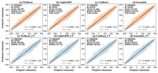
Figure 5.
The validation results of the test sets of the four models (a–d) and the 10-fold CV results (e–h): (a,e) XGBoost model, (b,f) LightGBM model, (c,g) CatBoost model and (d,h) Ensemble model. The orange areas represent the distribution of test set data points, while the blue areas indicate the distribution of 10-fold CV data points.
Although all four models produced GWSAs estimates below the actual values, the ensemble model’s trend-line slope of 0.94 was closest to the ideal value of 1. Relative to the other models, this model effectively mitigated bias and variance in its estimates, yielding predictions that more closely aligned with the actual values. Furthermore, we also compared the performance of the four models in each month (see Table 2), and calculated the 95% confidence intervals of the corresponding indicators (see Table A4) through the non-parametric bootstrap method (1000 resamplings) to enhance the statistical credibility of the differences. Among them, each model had the best fitting effect in June and the worst fitting effect in February, and the model performance had certain monthly fluctuations. This seasonal fluctuation may be related to the complication of surface hydrological signals caused by winter snow cover. Nevertheless, among all months, the ensemble model had the best overall performance, and its R2 and RMSE indicators were better than those of the single models. For example, in June, when the model performed best, the R2 of the ensemble model reached 0.948, which was better than the XGBoost model (R2: 0.928), the LightGBM model (R2: 0.939), and the CatBoost model (R2: 0.931); at the same time, the RMSE decreased to 22.354 mm, which was significantly lower than that of the XGBoost (RMSE: 26.443 mm), LightGBM (RMSE: 24.335 mm), and CatBoost (RMSE: 25.843 mm) models. From the overall monthly data, compared with the traditional single models, the Ensemble model significantly reduced the prediction error (RMSE decreased by about 12.3%), which also confirmed the conclusion that ensemble learning can effectively enhance the robustness of the model [45]. Specifically, the R2 value of the ensemble model remained above 0.915 in all months, and the RMSE was stably lower than 25 mm, which was significantly better than other single models. This indicates that the ensemble model can not only effectively capture the potential patterns between the data but also that is has a strong anti-noise capacity and maintains a high prediction performance even when the sample characteristics are quite different.
Table 2.
The 10-fold CV results of the four models on the monthly scale.
It should be noted that the ensemble model constructed based on the Stacking framework did not significantly improve the performance of single models such as XGBoost, LightGBM, and CatBoost. This is because the primary objective of the Stacking ensemble method is not to learn the statistical relationship between the explanatory variables and GWSAs, but to take the output results of the XGBoost, LightGBM, and CatBoost models as input. By learning the nonlinear differences between the predicted values and actual values across these diverse machine learning models, it aims to correct and integrate the biases and variances of their output results, thereby producing a prediction result that is closer to the true value [56].
3.1.2. Time Series Comparison
With the aim of evaluating the accuracy of the ensemble learning method when predicting the monthly average value of GWSAs at the time series level, we compared the monthly sequence variation in GWSAs from 2010 to 2020 before downscaling (original resolution of 0.25° × 0.25°) and after downscaling (resolution of 1 km × 1 km) (as shown in Figure 6). From the overall trend, the two curves are basically consistent regarding the peak and valley values, and the variation range of the time series is similar, both showing a typical seasonal cycle change: the peaks of GWSAs often occur in winter and early spring, while the troughs are manifested in summer and early autumn. This suggests that the high-resolution results after downscaling can effectively capture the seasonal cycle signal and interannual fluctuation trends in the original data, and are suitable for predicting the variation in groundwater reserves under the current data flow and results.

Figure 6.
The monthly average time series variation for GWSAs from 2010 to 2020.
3.1.3. Validation of In Situ Measurements
To additionally confirm the precision of the monthly GWSAs dataset with high spatial resolution after downscaling, we calculated the Pearson correlation coefficient (CC) between the GWLAs of 431 monitoring wells and the corresponding GWSAs pixels at 0.25° and 1 km spatial resolutions, respectively. The correlation analysis results of the monthly time series are shown in Figure 7. In particular, to guarantee the scientificity and precision of the correlation estimates, this study adopted a double significance test (confidence levels of 99% and 95%) to determine whether the correlation between the GWSAs of each monitoring well and the measured data was significant.

Figure 7.
The distribution of CC between GWSAs of the CONUS and the measured data: (a) GWSAs at the original resolution (0.25° × 0.25°); (b) GWSAs after downscaling (1 km × 1 km).
The results of the significance tests show that at the 99% significance level, 240 stations showed significant correlations before downscaling, while 269 stations showed significant correlations after downscaling. At the 95% significance level, there were an additional 42 stations showing significant correlations before downscaling, and an additional 21 stations reaching the significance standard after downscaling. It can be seen from Figure 7 that the monitoring wells with a relatively strong correlation (CC > 0.5) were mainly concentrated in areas with relatively concentrated precipitation, frequent agricultural irrigation activities or a dense population. Overall, a total of 282 stations showed significant correlations at least at the 95% significance level before downscaling, while this number increased to 290 stations after downscaling. Moreover, about 61.7% of the data points of the monitoring wells showed higher correlations. Compared with the original monthly GWSAs data with a spatial resolution of 0.25°, the overall correlation coefficient increased by approximately 18.7%. Moreover, it can be seen from the seasonal distribution of CC in Figure A1 that the correlation is the best in summer, with 34.80% of the stations significantly correlated with the measured data at least at the 95% significance level, while the correlation is the worst in winter, with only 13.46% of the stations showing significant correlation. This seasonal difference indicates that during the peak irrigation period in summer, the model has the strongest simulation ability for groundwater dynamics, possibly because the input meteorological and water quantity parameters can better capture the influences of evapotranspiration and artificial irrigation. However, in winter or the soil freezing period, the correlation systematically decreases, indicating that at this time the model fails to fully reflect factors such as the low-temperature freeze–thaw process, scarce precipitation, and weakened irrigation.
On the whole, the correlation with the measured data after downscaling remained comparable or even slightly improved compared to that before downscaling, indicating that the refinement processing did not destroy the main information of the original GRACE data. Moreover, in urbanized and irrigation-intensive areas, due to the introduction of more high-resolution features such as hydrology, meteorology, and human activities, the model’s ability to dynamically describe groundwater was further improved.
3.2. Sensitivity Analysis of Model Performance
3.2.1. Variability in Relative Importance of Explanatory Variables
In this study, through the distribution of the relative importance of explanatory variables in the three machine learning models, namely XGBoost, LightGBM, and CatBoost (as shown in Figure 8), a systematic analysis was conducted on the differences in the contribution of input variables to the prediction of GWSAs, revealing the driving role of each factor in the model.

Figure 8.
The relative importance of each explanatory variable in (a) XGBoost, (b) LightGBM and (c) CatBoost models.
The results of the three machine learning models showed that the spatiotemporal factors (Longitude, Latitude, and time) had the highest importance in GWSAs prediction (average contribution > 30%), which is highly consistent with the spatiotemporal non-stationarity characteristics and regional distribution laws of the groundwater system [2,21,57]. Especially in the CatBoost model, the average contributions of longitude, latitude, and time were 32.75%, 24.14%, and 20.91%, respectively. This phenomenon indicates that, in GWSAs prediction, the CatBoost model fully considers the comprehensive influence of spatiotemporal factors, enabling it to more accurately capture the spatiotemporal dynamic heterogeneity of groundwater storage. This in-depth exploration of spatiotemporal factors enables the CatBoost model to show stronger predictive ability in specific situations. In contrast, the LightGBM model had a more significant dependence on time features. The average contribution of its time variable was 14.92%, while the average contributions of longitude and latitude were 18.02% and 15.32%, respectively. This demonstrates that the LightGBM model has a strong ability to capture the changes in seasonal and periodic hydrological processes, but is marginally weaker than the CatBoost model in the utilization of spatial features. Compared with the other two models, the XGBoost model demonstrates a relatively balanced distribution of the importance of explanatory variables. This balance enables it to effectively identify the influence degree of each variable on GWSAs, avoid excessive dependence on a certain variable, and thereby enhance the comprehensive understanding of groundwater storage changes. In terms of spatiotemporal factors, the average contributions of longitude and latitude in the XGBoost model were 12.38% and 10.58%, respectively, while the average contribution of time was 9.96%, indicating balanced attention to spatiotemporal features. Comparatively, this indicates that the XGBoost model does not overly bias towards a certain direction in the utilization of spatial and temporal features, but provides a stable modeling strategy in GWSAs prediction by balancing the processing of spatial differentiation and temporal changes.
Besides spatiotemporal factors, the coupled driving factors across multiple earth spheres (atmosphere, hydrosphere, and pedosphere) exhibited secondary important contributions to the prediction of GWSAs. The XGBoost, LightGBM, and CatBoost models captured the driving effect of the multi-sphere coupling process on groundwater storage change through their respective unique feature selection mechanisms. Specifically, the XGBoost model showed stronger sensitivity to soil texture parameters in the pedosphere. It showed higher sensitivity to land cover type (LC), clay content at a depth of 30 cm (ClayB30), and sand content (SandB30), with average contribution degrees of 9.73%, 8.43%, and 8.13%, respectively. This feature may stem from the fact that the gradient boosting mechanism of the XGBoost model has a stronger ability to capture discrete categorical variables (such as LC) and nonlinear features (such as soil texture parameters) [58]. This finding indicates that the XGBoost model is more effective in analyzing the infiltration differences caused by surface cover changes and the influence of soil water-holding characteristics on the groundwater recharge process [59,60]. In contrast, the LightGBM and CatBoost models showed higher dependence on hydrological process variables. Both of them assigned higher feature importance to total precipitation (Train), runoff (Runoff), and surface soil water content (Swvl1). The average contribution degrees of the LightGBM model were 7.56%, 6.50%, and 6.90%, respectively, and those of the CatBoost model were 2.59%, 2.64%, and 3.43%, respectively. This characteristic may stem from the different model architecture characteristics of the two: The “Leaf-Wise” tree growth strategy of the LightGBM model enables it to have a stronger ability to capture the temporal changes in continuous hydrological variables [61]; meanwhile, the CatBoost model strengthens the learning of temporal features by reducing the prediction shift that occurred during the training process [55], thus enabling it to better manage categorical variables and continuous variables [62].
It is worth noting that, as can be seen from Figure 8, the common sensitivity of the three models to the surface pressure (SP) of the atmosphere revealed the special status of this variable (XGBoost: 8.37%; LightGBM: 7.59%; CatBoost: 6.91%). As a comprehensive meteorological variable, changes in SP may simultaneously affect multiple climatic factors such as precipitation, evapotranspiration, and temperature, thereby having a more complex and far-reaching impact on the groundwater system.
3.2.2. Dynamic Characteristics of Base Models Weight Allocation
In order to enable the weight distribution to reflect the differences in the performance of different models when the seasons, meteorological and hydrological conditions change, this study adopted the ADWA approach, and combined the error feedback factor to calculate the weight ratios of the XGBoost, LightGBM and CatBoost models in the ensemble framework month by month, to quantify the prediction contribution of each base model in different time periods. Figure 9 illustrates the weight distribution of the three base models in the ensemble model for each month.

Figure 9.
Weight proportion of the three machine learning models (XGBoost, LightGBM, and CatBoost) in the ensemble model for each month.
Considering the overall dynamics of weight allocation, the standard deviations of the weights of the three base models, namely LightGBM, XGBoost, and CatBoost, in the 12-month prediction task were 0.20%, 0.42%, and 0.38%, respectively, while the total weight range of the ensemble model was 5.11 percentage points. This indicates that the ensemble model can adaptively integrate the advantages of each base model through the ADWA approach. Even if each model had differences in processing spatiotemporal features, the weight fluctuations remained within a small range, avoiding the situation of overall prediction instability caused by the excessive bias of a single model. At the same time, the smaller standard deviation shows that the model can achieve effective optimization in different time periods, thereby effectively reducing the interference of noise and abnormal data when facing tasks with high nonlinearity and spatiotemporal complexity such as hydrological data.
3.3. Comparative Analysis of Coarse and Fine Resolution Data
Figure 10 shows the downscaling comparison of the total average GWSAs in CONUS from 2010 to 2020. It can be seen from the comparison results that the low-resolution (0.25° × 0.25°) and the high-resolution (1 km × 1 km) data have a high consistency in the overall spatial distribution characteristics. For example, the positive anomaly zone in the northeastern Great Lakes region and the negative anomaly areas in the central and southern High Plains and the southwestern Central Valley all exist under both resolutions, indicating the dominant role of large-scale hydrological processes. However, the high-resolution data, as shown in Figure 10a,c,e, have obvious local differences in spatial details. This difference is mainly reflected in the degree of data smoothing, local outliers, and the transition of spatial boundaries.

Figure 10.
Comparison of downscaled 2010–2020 total mean GWSAs: (a,c,e) downscaled GWSAs (1 km × 1 km); (b,d,f) original GWSAs (0.25° × 0.25°).
From the perspective of spatial details, the downscaled 1 km resolution data, due to the smaller pixel size, has more delicate spatial variations, clearer boundaries for local areas, and is more sensitive to the changes in local outliers. This has obvious advantages when revealing the complex hydrological processes within the region. In contrast, the original 0.25° resolution data, due to the lower resolution, often shows phenomena such as transitional blurring at the regional edges and the smoothing of local peak and valley values. For example, in some areas with complex terrain or uneven precipitation and evapotranspiration, high-resolution data can better capture local abnormal high or low values, while low-resolution data may underestimate or overestimate local peaks or valleys to a certain extent, thereby leading to the cumulative effect of numerical errors in specific time periods.
The comparison of coarse and fine resolutions also reflects the differences in the spatial positioning accuracy. High-resolution data can accurately reflect the changes in groundwater reserves on a small scale, for example, in coastal areas, river confluences, or urban fringe areas, which are greatly affected by local hydrology, climate, and human activities, and their GWSA values will fluctuate significantly. However, low-resolution data, often due to spatial averaging, ignore these small but crucial regional differences and do not accurately reflect the dynamic changes in groundwater. This local difference brought by resolution is of great significance in regional management decisions because only fine-scale data can provide a more targeted basis for local water resource regulation.
3.4. Analysis of the Fine-Scale Spatiotemporal Distribution of GWSAs
Based on the 1 km resolution GWSAs data generated by the ensemble model, this study systematically analyzed the spatiotemporal distribution characteristics and evolution patterns of GWSAs in CONUS at annual, monthly and seasonal scales from 2010 to 2020, revealing the regional heterogeneity, seasonal fluctuations and long-term trends in GWSAs.
It can be seen from Figure 11 that the annual average GWSAs in the CONUS as a whole presents significant regional differentiation characteristics. The northern high plains and the areas near the Great Lakes in the study area remained significant positive anomaly areas all year round. The GWSA value in these regions ranged from 160 to 320 mm, with central areas exceeding 360 mm. However, in the two groundwater depletion hotspots in the southwestern California Central Valley and the central–southern High Plains and the surrounding areas of the study area, the groundwater reserves showed a significant negative deviation from the average value of the base period (2004–2009), remaining in a negative anomaly of −80 to −200 mm for a long time. The local area was even lower than −200 mm, which is consistent with the research results of Scanlon et al. [63] on the High Plains and Central Valley of the United States. In contrast, the southeastern states of the United States such as Florida and Georgia mainly showed positive anomalies on the whole, but the values were relatively lower than those in the central–northern part, fluctuating between 0 and 120 mm in most years, mainly governed by the combined effects of local precipitation variability and water demand.

Figure 11.
Annual distribution of GWSAs output by the ensemble model.
Combining the monthly (see Figure 12) and seasonal (see Figure 13) distribution of GWSAs, the distribution of GWSAs in each month shows a significant seasonal variation trend. From January to April, the overall GWSA value in the southeastern plains and coastal areas of the study area gradually rises to a relatively high level of 100–240 mm, reaching the peak in April, showing that snowmelt and spring precipitation have a positive effect on groundwater recharge and the initial accumulation stage of groundwater reserves. Meanwhile, the two groundwater depletion hotspots in the southwestern Central Valley and the central–southern high plains and the surrounding areas usually remain within the negative anomaly range of −80 to −160 mm, and in individual months, it can approach or even be lower than −160 mm.

Figure 12.
Monthly distribution of GWSAs output by the ensemble model.

Figure 13.
Seasonal distribution of GWSAs output by the ensemble model: Spring (March–May), Summer (June–August), Autumn (September–November), Winter (December–February).
From May to September, the GWSAs in the study area as a whole presented a trend of “turning from positive to weak and spreading from negative”, reaching a relative low point in September. During this period, the GWSAs in the northern high plain area significantly weakened, with positive anomalies mostly concentrated in the range of 80–160 mm, and the surrounding areas of Nebraska dropped to 0–80 mm, which was directly related to the sharp increase in irrigation demand during the crop growth period. With the combined effects of multiple factors such as enhanced evapotranspiration, increased agricultural irrigation demand, increased human water withdrawal, and the uneven spatiotemporal distribution of precipitation on groundwater recharge [64], the GWSAs in the central–eastern plain area gradually dropped to nearly 0 mm, and negative values appeared in regions such as Kentucky and Tennessee. The GWSAs in densely populated areas in the northeast, such as New York, Vermont, and Connecticut, dropped to −80 mm. The negative anomaly was more significant in the depleted hotspots in the southwest and central-south during this stage, with most areas being lower than −120 mm, and the range of negative anomaly areas gradually expanded to the western coastal areas.
From October to December, the overall GWSAs showed a gradual callback trend. Due to increased precipitation recharge and reduced agricultural water use, the GWSAs in most areas rebounded by 40–80 mm, but overexploited areas such as the Central Valley and the central–southern High Plain still maintained a relatively significant negative anomaly (−80–160 mm), indicating that natural recharge could not easily counteract the long-term exploitation pressure. The spatial gradient of anomaly values in each region at this stage tended to be gentle, indicating that the groundwater system gradually recovered to a more balanced state after experiencing intense fluctuations in the medium term.
4. Discussion
4.1. Comparison of Existing Downscaling Models for GWSAs
This study adopted three machine learning models, namely XGBoost, LightGBM, and CatBoost, as the base models. Under the Stacking ensemble framework, the ADWA approach was introduced, and the ridge regression model was used to optimize and fuse the outputs of different models, achieving the complementary advantages of multiple models. First of all, the ensemble model in this paper demonstrated the superior ability to evaluate GWSAs. The ensemble model achieved a monthly average R2 of 0.931 and NSE of 0.936 in 10-fold CV, with R2 remaining above 0.915 across all months, outperforming most existing models. This includes the annual artificial neural network model (NSE: 0.0391–0.7511) constructed by Miro et al. [15], the annual random forest model (NSE: 0.68) constructed by Li et al. [65], the annual XGBoost model (R2: 0.77–0.89) and random forest model (R2: 0.74–0.86) constructed by Zhang et al. [41], and the annual random forest model (R2: 0.85) proposed by Ghaffari et al. [66].
Secondly, the ensemble model developed in this study generated monthly 1 km resolution results. It effectively integrated the individual strengths of various ML models in capturing nonlinear relationships, feature interactions, and handling high-dimensional complex data, thereby better meeting the requirements of high-precision groundwater monitoring and scientific management. As far as we know, little research has utilized ensemble learning methods for groundwater storage monitoring with spatial resolutions exceeding 1 km. For example, Yin et al. [48] constructed a Bayesian ensemble model integrating an artificial neural network, the support vector machine, and response surface regression to finely predict groundwater storage changes, achieving a regional average R2 of 0.928. However, their input data were derived from the C2VSim model grids and were statistically aggregated by sub-regions with monitoring stations. Moreover, their approach was limited to the Central Valley of California, hindering the detection of local heterogeneity and anomalies.
4.2. Analysis of the Spatiotemporal Heterogeneity of High-Resolution GWSAs
In this study, the monthly 1 km high spatiotemporal resolution GWSAs dataset generated revealed significant spatiotemporal heterogeneity in the CONUS, surpassing traditional GRACE products in spatial detail and mechanistic resolution. A comparison of the long-term GWSAs trends (Figure 6) and annual distributions (Figure 11) showed a long-term seasonal cycle fluctuation in the GWSAs. Among them, the GWSAs in the southern High Plains and the Central Valley of California presented a long-term negative anomaly (−80 to −200 mm), but the overall trend was relatively stable. From the overall trend in Figure 6, the GWSAs show a slightly downward trend, and in the long term, groundwater is in a state of continuous consumption. Although it is still in a downward trend after 2015, the rate of decline has changed from −4.56 mm/year to −3.33 mm/year, showing that it has slowed down. This phenomenon is consistent with the research results of Ashraf et al. [22] on the major aquifers in the United States: Although the groundwater storage of the aquifers in the southwestern and central–southern parts of the United States shows a downward trend, the groundwater storage trend of most of the other aquifers is stable or slightly rising. Monthly (Figure 12) and seasonal (Figure 13) GWSAs distributions demonstrated that the areas with relatively abundant groundwater reserves were mainly concentrated in the areas with rich annual precipitation, moderate soil permeability, and good irrigation recharge conditions (such as the northern high plains, the Great Lakes region, Florida, etc.). In contrast, arid/semi-arid areas (e.g., central–southern High Plains, California Central Valley) showed persistent negative anomalies, highlighting the imbalance between exploitation and recharge [8].
Groundwater flows slowly, especially in comparison with surface water systems or the atmosphere. Likewise, the stress propagation and reactions in groundwater systems exhibit a considerably slower pace compared to those in surface water systems or the atmosphere [17]. Additionally, the retention period of groundwater is usually significantly longer than that of surface water. These general characteristics imply that the key issues in groundwater systems are slow propagation, detection difficulties, and remediation complexities [8]. Therefore, water resource planning and management strategies should be based on a long-term perspective, systematically understanding the hydraulic linkage between surface water and groundwater systems. Enhancing the early identification of slow groundwater changes via high-resolution monitoring, relying on long-term data for trend analysis, and deepening water cycle linkage studies through multi-source data fusion can provide scientific support for sustainable groundwater management.
4.3. Uncertainty Analysis
Our study observed that there were significant differences in the predictive performance of different base models (XGBoost, LightGBM and CatBoost) in each month, which might stem from the differences in model structure and the different capacity of each model to capture explanatory variables of different resolutions and types. In the regularization system, XGBoost explicitly introduces the L2 regularization term, CatBoost implicitly constrains the model complexity through the symmetrical tree structure, and LightGBM relies on the natural regularization of histogram merging, which leads to substantial differences in the control paths of model complexity [55]. These structural differences lead to the model having different performances in handling feature interaction, depth control and generalization, and may also introduce different degrees of error and uncertainty. The input data used (such as population distribution, evapotranspiration, soil texture, etc.) have certain spatial and temporal resolution limitations, which may not be able to fully capture the changes at the local scale, affecting the accuracy of the model. Under the current research conditions, complex geological elements such as the unique fracture characteristics of the local aquifer and the characteristics of the unsaturated zone may increase the uncertainty of the results through the interaction with the model parameter system [7]. The objective difficulties that exist in the data representation of such heterogeneous stratum characteristics deserve special attention in follow-up studies.
4.4. Study Limitations and Future Research Directions
Although this study achieved positive results in improving the spatial resolution of GWSAs, there are still some limitations. First, GRACE/GRACE-FO data, while critical for terrestrial water storage inversion, are limited by a low spatial resolution and inherent noise, particularly in complex terrains. Although downscaling via ensemble machine learning and multi-source datasets (e.g., GTWS-MLrec, GLDAS, ERA5-Land) mitigates these issues, residual uncertainties from data fusion may propagate into the final estimates.
Second, while validated extensively in the CONUS, the performance of models may vary in regions with distinct hydrogeological and anthropogenic profiles (e.g., North China Plain, characterized by intensive irrigation and seasonal precipitation) [67,68,69]. Therefore, when extending the model globally, the model method is universal, but the model parameters need to be recalibrated specifically in combination with local observation data. For areas with scarce observation wells, the well-validated model parameters in CONUS can be used as the initial weights through the cross-regional transfer learning strategy, and fine-tuned on a small amount of local data to reduce the dependence on the high-density monitoring network.
Third, the inherent “black-box” nature of ML methods limits the physical interpretability of their predictions. Future research should integrate process-based hydrological models with high-resolution socio-environmental data [70]. On this basis, the predictor set should be further expanded, including publicly available monitoring data of the groundwater pumping rate, high-precision land subsidence information combined with satellite remote sensing and ground observations, as well as other publicly available geophysical data. This multi-source data fusion can not only enhance the physical meaning of the model, but also deepen our understanding of the response mechanism of the groundwater system under varying human–water interaction regimes, and provide more scientific and reliable decision support for the formulation of sustainable groundwater management strategies.
5. Conclusions
In this article, based on the 0.25° resolution GWSAs data derived from the GRACE satellite and GLDAS model, we combined the XGBoost, LightGBM and CatBoost models, and used multi-source data to construct a Stacking-based high-resolution ensemble model by introducing the ADWA approach. The ensemble model has been successfully applied to the CONUS, generating monthly GWSAs distribution maps at a 1 km spatial resolution, and analyzing the variation laws and distribution of GWSAs at a high spatiotemporal resolution.
Relative to other studies, the ensemble model demonstrated superior estimation accuracy, with R2, RMSE, MAE, and NSE values of 0.929, 25.232 mm, 19.125 mm, and 0.936, respectively, verifying its strong generalization abilities under complex spatiotemporal heterogeneity conditions. To sum up, the ensemble machine learning approach not only significantly enhances the precision of monitoring GWSAs but also offers a novel solution for the downscaling of GRACE inversion data. Furthermore, it provides robust technical support and a reliable data foundation for the sustainable management of groundwater resources.
Based on the monthly GWSAs dataset at a 1 km spatial resolution, this study reveals the significant regional differentiation characteristics of groundwater storage changes in the continental United States. The central–southern High Plains and the Central Valley of California in the CONUS show long-term negative anomalies (−80 to −200 mm), which are directly related to overexploitation and drought stress; the northern High Plains and the Great Lakes region maintain a relatively high positive anomaly (160 to 320 mm) due to sufficient natural recharge. The downscaling results clearly depict the characteristics of seasonal fluctuations, such as the peak driven by spring snowmelt recharge and the trough caused by summer irrigation consumption. Compared with the original GRACE data with a resolution of 0.25°, the applicability of the downscaled products for local groundwater dynamic monitoring and management is significantly enhanced, providing a refined spatial basis for regional water resource management.
To sum up, the refined downscaling of GRACE-derived GWSAs data using the ensemble machine learning model can not only break through the inherent resolution limitations of GRACE gravity satellite data, but also effectively integrate multi-source geographic information to describe the dynamic evolution process of groundwater at a higher spatiotemporal accuracy. Thus, it can assist in formulating more targeted groundwater regulation and recharge strategies, providing an important basis for local water resource management departments to identify hotspots prone to water resource risks.
Author Contributions
Conceptualization, Y.Y. and D.S.; methodology, Y.Y. and D.S.; software, X.W.; validation, Y.C., B.Z. and H.D.; formal analysis, Y.Y.; investigation, X.W.; resources, H.D.; data curation, B.Z.; writing—original draft preparation, Y.Y. and D.S.; writing—review and editing, Y.Y., D.S. and H.D.; visualization, Y.C.; supervision, H.D.; project administration, D.S.; funding acquisition, Y.Y. All authors have read and agreed to the published version of the manuscript.
Funding
This research was funded by the National Natural Science Foundation of China, grant number 52079101 and 2024 Ningbo Municipal Public Welfare Research Plan Project, grant number 2024S008.
Data Availability Statement
The data presented in this study are available upon request from the corresponding author. The data are not publicly available due to privacy or ethical restrictions.
Acknowledgments
The authors thank the free open-access datasets used in this study. ERA5 reanalysis data from the European Center for Medium-Range Weather Forecasts (ECMWF). GLDAS data from the Goddard Earth Sciences Data and In-formation Services Center (GESDISC).
Conflicts of Interest
Heng Dong was employed by Zhejiang Spatiotemporal Sophon Bigdata Co., Ltd. The remaining authors declare that the research was conducted in the absence of any commercial or financial relationships that could be construed as a potential conflict of interest.
Appendix A
Table A1.
Missing months from the GRACE/GRACE-FO missions during 2010–2020.
Table A1.
Missing months from the GRACE/GRACE-FO missions during 2010–2020.
| Mission Period | Missing Months (201001–202012) |
|---|---|
| GRACE | 201101, 201106, 201111, 201204, 201205, 201210, 201303, 201308, 201309, 201402, 201407, 201412, 201505, 201507, 201510, 201511, 201602, 201604, 201609, 201610, 201702 |
| Gap Period | 201706, 201707, 201708, 201709, 201710, 201711, 201712, 201801, 201802, 201803, 201804, 201805 |
| GRACE-FO | 201808, 201809, 201902 |
Table A2.
The reanalysis data variables.
Table A2.
The reanalysis data variables.
| Variable (Acronym) | Unit | Spatiotemporal Resolution | Data Source |
|---|---|---|---|
| total precipitation (Train) | m | Monthly; 0.25° × 0.25° | ECMWF ERA5-Land (https://doi.org/10.24381/cds.68d2bb30 (accessed on 10 November 2024)) |
| 2m temperature (T2m) | K | ||
| Runoff (Runoff) | m | ||
| surface pressure (SP) | Pa | ||
| surface net solar radiation (Snsr) | J/m2 | ||
| 0–7 cm volumetric soil water (Swvl1) | m3/m3 | ||
| 7–28 cm volumetric soil water (Swvl2) | m3/m3 | ||
| 28–100 cm volumetric soil water (Swvl3) | m3/m3 | ||
| 100–289 cm volumetric soil water (Swvl4) | m3/m3 |
Table A3.
Grid search ranges for generalized hyperparameters of the three base models.
Table A3.
Grid search ranges for generalized hyperparameters of the three base models.
| Generalized Hyperparameter | Candidate Range |
|---|---|
| n_estimators | [200, 250, 300, 350, 400, 450, 500, 550, 600] |
| max_depth | [5, 6, 7, 8, 9, 10, 11, 12, 13] |
| learning_rate | [0.01, 0.03, 0.05, 0.08, 0.1] |

Figure A1.
The seasonal distribution of CC between the downscaled GWSAs and the measured data: Spring (March–May), Summer (June–August), Autumn (September–November), Winter (December–February).
Table A4.
95% Confidence intervals of monthly R2 and RMSE for four models (bootstrap 1000).
Table A4.
95% Confidence intervals of monthly R2 and RMSE for four models (bootstrap 1000).
| Month | XGBoost (95% CI) | LightGBM (95% CI) | CatBoost (95% CI) | Ensemble (95% CI) | ||||
|---|---|---|---|---|---|---|---|---|
| R2 | RMSE | R2 | RMSE | R2 | RMSE | R2 | RMSE | |
| Mon01 | [0.895, 0.897] | [27.649, 27.958] | [0.912, 0.914] | [25.268, 25.462] | [0.898, 0.901] | [27.192, 27.483] | [0.925, 0.928] | [23.236, 23.474] |
| Mon02 | [0.880, 0.883] | [27.846, 28.163] | [0.897, 0.899] | [25.860, 26.074] | [0.884, 0.888] | [27.332, 27.611] | [0.914, 0.917] | [23.583, 23.767] |
| Mon03 | [0.891, 0.894] | [29.173, 29.432] | [0.910, 0.912] | [26.581, 26.804] | [0.901, 0.903] | [27.915, 28.171] | [0.925, 0.927] | [24.231, 24.474] |
| Mon04 | [0.894, 0.897] | [28.297, 28.557] | [0.912, 0.915] | [25.718, 25.982] | [0.902, 0.904] | [27.206, 27.469] | [0.927, 0.929] | [23.378, 23.629] |
| Mon05 | [0.910, 0.912] | [27.713, 27.984] | [0.924, 0.926] | [25.497, 25.719] | [0.917, 0.920] | [26.574, 26.925] | [0.936, 0.938] | [23.321, 23.473] |
| Mon06 | [0.926, 0.929] | [26.291, 26.588] | [0.938, 0.940] | [24.180, 24.457] | [0.930, 0.932] | [25.749, 25.946] | [0.947, 0.949] | [22.249, 22.468] |
| Mon07 | [0.912, 0.914] | [26.345, 26.664] | [0.925, 0.927] | [24.222, 24.558] | [0.916, 0.919] | [25.587, 25.912] | [0.936, 0.939] | [22.300, 22.589] |
| Mon08 | [0.900, 0.903] | [27.537, 27.827] | [0.917, 0.919] | [25.161, 25.366] | [0.909, 0.912] | [26.290, 26.520] | [0.930, 0.932] | [23.067, 23.293] |
| Mon09 | [0.887, 0.890] | [29.642, 29.973] | [0.910, 0.912] | [26.580, 26.796] | [0.902, 0.905] | [27.650, 27.863] | [0.928, 0.930] | [23.788, 23.944] |
| Mon10 | [0.886, 0.888] | [29.172, 29.550] | [0.908, 0.911] | [26.062, 26.413] | [0.899, 0.902] | [27.383, 27.717] | [0.923, 0.925] | [23.953, 24.253] |
| Mon11 | [0.902, 0.905] | [28.163, 28.536] | [0.921, 0.924] | [25.346, 25.624] | [0.913, 0.916] | [26.517, 26.866] | [0.936, 0.938] | [22.768, 22.976] |
| Mon12 | [0.896, 0.899] | [28.132, 28.519] | [0.916, 0.918] | [25.391, 25.712] | [0.905, 0.908] | [26.941, 27.273] | [0.929, 0.931] | [23.287, 23.503] |
References
- World Economic Forum. The Global Risks Report 2024; World Economic Forum: Cologny/Geneva, Switzerland, 2024. [Google Scholar]
- Konikow, L.F. Contribution of global groundwater depletion since 1900 to sea-level rise. Geophys. Res. Lett. 2011, 38. [Google Scholar] [CrossRef]
- Condon, L.E.; Maxwell, R.M. Evaluating the relationship between topography and groundwater using outputs from a continental-scale integrated hydrology model. Water Resour. Res. 2015, 51, 6602–6621. [Google Scholar] [CrossRef]
- Chen, J.; Famigliett, J.S.; Scanlon, B.R.; Rodell, M. Groundwater Storage Changes: Present Status from GRACE Observations. Surv. Geophys. 2016, 37, 397–417. [Google Scholar] [CrossRef]
- Thomas, B.F.; Famiglietti, J.S.; Landerer, F.W.; Wiese, D.N.; Molotch, N.P.; Argus, D.F. GRACE Groundwater Drought Index: Evaluation of California Central Valley groundwater drought. Remote Sens. Environ. 2017, 198, 384–392. [Google Scholar] [CrossRef]
- Gleeson, T.; Cuthbert, M.; Ferguson, G.; Perrone, D. Global Groundwater Sustainability, Resources, and Systems in the Anthropocene. Annu. Rev. Earth Planet. Sci. 2020, 48, 431–463. [Google Scholar] [CrossRef]
- Zell, W.O.; Sanford, W.E. Calibrated Simulation of the Long-Term Average Surficial Groundwater System and Derived Spatial Distributions of its Characteristics for the Contiguous United States. Water Resources Research 2020, 56, e2019WR026724. [Google Scholar] [CrossRef]
- Konikow, L.F. Long-Term Groundwater Depletion in the United States. Groundwater 2015, 53, 2–9. [Google Scholar] [CrossRef]
- Vasilis, G.; Carlo Nike, B. Mediterranean marine caves: A synthesis of current knowledge. In Oceanography and Marine Biology; CRC Press: Boca Raton, FL, USA, 2021; Volume 59, pp. 1–88. [Google Scholar] [CrossRef]
- Wynne, J.J.; Howarth, F.G.; Mammola, S.; Ferreira, R.L.; Cardoso, P.; Lorenzo, T.D.; Galassi, D.M.P.; Medellin, R.A.; Miller, B.W.; Sánchez-Fernández, D.; et al. A conservation roadmap for the subterranean biome. Conserv. Lett. 2021, 14, e12834. [Google Scholar] [CrossRef]
- Mammola, S.; Meierhofer, M.B.; Borges, P.A.V.; Colado, R.; Culver, D.C.; Deharveng, L.; Delić, T.; Di Lorenzo, T.; Dražina, T.; Ferreira, R.L.; et al. Towards evidence-based conservation of subterranean ecosystems. Biol. Rev. 2022, 97, 1476–1510. [Google Scholar] [CrossRef] [PubMed]
- Xue, D.; Gui, D.; Ci, M.; Liu, Q.; Wei, G.; Liu, Y. Spatial and temporal downscaling schemes to reconstruct high-resolution GRACE data: A case study in the Tarim River Basin, Northwest China. Sci. Total Environ. 2024, 907, 167908. [Google Scholar] [CrossRef] [PubMed]
- Arshad, A.; Mirchi, A.; Samimi, M.; Ahmad, B. Combining downscaled-GRACE data with SWAT to improve the estimation of groundwater storage and depletion variations in the Irrigated Indus Basin (IIB). Sci. Total Environ. 2022, 838, 156044. [Google Scholar] [CrossRef] [PubMed]
- Ali, S.; Liu, D.; Fu, Q.; Cheema, M.J.M.; Pham, Q.B.; Rahaman, M.M.; Dang, T.D.; Anh, D.T. Improving the Resolution of GRACE Data for Spatio-Temporal Groundwater Storage Assessment. Remote Sens. 2021, 13, 3513. [Google Scholar] [CrossRef]
- Miro, M.E.; Famiglietti, J.S. Downscaling GRACE Remote Sensing Datasets to High-Resolution Groundwater Storage Change Maps of California’s Central Valley. Remote Sens. 2018, 10, 143. [Google Scholar] [CrossRef]
- Feng, W.; Shum, C.K.; Zhong, M.; Pan, Y. Groundwater Storage Changes in China from Satellite Gravity: An Overview. Remote Sens. 2018, 10, 674. [Google Scholar] [CrossRef]
- Rodell, M.; Velicogna, I.; Famiglietti, J.S. Satellite-based estimates of groundwater depletion in India. Nature 2009, 460, 999–1002. [Google Scholar] [CrossRef] [PubMed]
- Tapley, B.D.; Bettadpur, S.; Ries, J.C.; Thompson, P.F.; Watkins, M.M. GRACE Measurements of Mass Variability in the Earth System. Science 2004, 305, 503–505. [Google Scholar] [CrossRef]
- Frappart, F.; Ramillien, G. Monitoring Groundwater Storage Changes Using the Gravity Recovery and Climate Experiment (GRACE) Satellite Mission: A Review. Remote Sens. 2018, 10, 829. [Google Scholar] [CrossRef]
- Richey, A.S.; Thomas, B.F.; Lo, M.H.; Reager, J.T.; Famiglietti, J.S.; Voss, K.; Swenson, S.; Rodell, M. Quantifying renewable groundwater stress with GRACE. Water Resour. Res. 2015, 51, 5217–5238. [Google Scholar] [CrossRef]
- Tapley, B.D.; Watkins, M.M.; Flechtner, F.; Reigber, C.; Bettadpur, S.; Rodell, M.; Sasgen, I.; Famiglietti, J.S.; Landerer, F.W.; Chambers, D.P.; et al. Contributions of GRACE to understanding climate change. Nat. Clim. Change 2019, 9, 358–369. [Google Scholar] [CrossRef]
- Rateb, A.; Scanlon, B.R.; Pool, D.R.; Sun, A.; Zhang, Z.; Chen, J.; Clark, B.; Faunt, C.C.; Haugh, C.J.; Hill, M.; et al. Comparison of Groundwater Storage Changes From GRACE Satellites With Monitoring and Modeling of Major US Aquifers. Water Resour. Res. 2020, 56, e2020WR027556. [Google Scholar] [CrossRef]
- Chen, J.; Cazenave, A.; Dahle, C.; Llovel, W.; Panet, I.; Pfeffer, J.; Moreira, L. Applications and Challenges of GRACE and GRACE Follow-On Satellite Gravimetry. Surv. Geophys. 2022, 43, 305–345. [Google Scholar] [CrossRef] [PubMed]
- Seyoum, W.M.; Milewski, A.M. Improved methods for estimating local terrestrial water dynamics from GRACE in the Northern High Plains. Adv. Water Resour. 2017, 110, 279–290. [Google Scholar] [CrossRef]
- He, Q.; Huang, B. Satellite-based mapping of daily high-resolution ground PM2.5 in China via space-time regression modeling. Remote Sens. Environ. 2018, 206, 72–83. [Google Scholar] [CrossRef]
- Atkinson, P.M. Downscaling in remote sensing. Int. J. Appl. Earth Obs. Geoinf. 2013, 22, 106–114. [Google Scholar] [CrossRef]
- Chen, F.R.; Liu, Y.; Liu, Q.; Li, X. Spatial downscaling of TRMM 3B43 precipitation considering spatial heterogeneity. Int. J. Remote Sens. 2014, 35, 3074–3093. [Google Scholar] [CrossRef]
- Sandip, M.; Pawan Kumar, J.; Rahul Dev, G. Regression-Kriging Technique to Downscale Satellite-Derived Land Surface Temperature in Heterogeneous Agricultural Landscape. IEEE J. Sel. Top. Appl. Earth Obs. Remote Sens. 2015, 8, 1245–1250. [Google Scholar] [CrossRef]
- Zhang, Q.; Shen, Z.; Xu, C.-Y.; Sun, P.; Hu, P.; He, C. A new statistical downscaling approach for global evaluation of the CMIP5 precipitation outputs: Model development and application. Sci. Total Environ. 2019, 690, 1048–1067. [Google Scholar] [CrossRef] [PubMed]
- Seon-Ho, K.; Jeongwoo, H.; Sankarasubramanian, A. Understanding the variability of large-scale statistical downscaling methods under different climate regimes. J. Hydrol. 2024, 641, 131818. [Google Scholar] [CrossRef]
- Mao, T.; Shangguan, W.; Li, Q.; Li, L.; Zhang, Y.; Huang, F.; Li, J.; Liu, W.; Zhang, R. A Spatial Downscaling Method for Remote Sensing Soil Moisture Based on Random Forest Considering Soil Moisture Memory and Mass Conservation. Remote Sens. 2022, 14, 3858. [Google Scholar] [CrossRef]
- Sun, Y.; Deng, K.; Ren, K.; Liu, J.; Deng, C.; Jin, Y. Deep learning in statistical downscaling for deriving high spatial resolution gridded meteorological data: A systematic review. ISPRS J. Photogramm. Remote Sens. 2024, 208, 14–38. [Google Scholar] [CrossRef]
- Bramha Dutt Vishwakarma, J.Z.N.S. Downscaling GRACE total water storage change using partial least squares regression. Sci. Data 2021, 8, 95. [Google Scholar] [CrossRef] [PubMed]
- Wei, H.; Xiaohan, Z.; Yi, W.; Lizhe, W.; Xiaohui, H.; Jun, L.; Sheng, W.; Weitao, C.; Xianju, L.; Ruyi, F.; et al. A survey of machine learning and deep learning in remote sensing of geological environment: Challenges, advances, and opportunities. ISPRS J. Photogramm. Remote Sens. 2023, 202, 87–113. [Google Scholar] [CrossRef]
- Yin, W.; Zhang, G.; Han, S.-C.; Yeo, I.-Y.; Zhang, M. Improving the resolution of GRACE-based water storage estimates based on machine learning downscaling schemes. J. Hydrol. 2022, 613, 128447. [Google Scholar] [CrossRef]
- Abdellatif, R.; Yassine, A.B.; Abdelhakim, A.; Mohamed, O.; Bouchra, B.; Hamza, O.; Yassine, B.; Lhoussaine, B.; Abdelghani, C. Groundwater level forecasting in a data-scarce region through remote sensing data downscaling, hydrological modeling, and machine learning: A case study from Morocco. J. Hydrol. Reg. Stud. 2023, 50, 101569. [Google Scholar]
- Sabzehee, F.; Amiri-Simkooei, A.R.; Iran-Pour, S.; Vishwakarma, B.D.; Kerachian, R. Enhancing spatial resolution of GRACE-derived groundwater storage anomalies in Urmia catchment using machine learning downscaling methods. J. Environ. Manag. 2023, 330, 117180. [Google Scholar] [CrossRef]
- Arman, A.; Mohammadali, O.; Zahra, H.; Mohammad, E.; Amin, Z.; Arash, G.; Andre, D.; Graham, E.F.; Mojtaba, S. Groundwater Level Modeling with Machine Learning: A Systematic Review and Meta-Analysis. Water 2022, 14, 949. [Google Scholar] [CrossRef]
- Ashraf, A.A.; Sakina, S.; Antoifi, A.; Salissou, M.; Lukumon, O. Applications of machine learning to water resources management: A review of present status and future opportunities. J. Clean. Prod. 2024, 441, 140715. [Google Scholar] [CrossRef]
- Fahad, H.; Paul, M.; Jason, D.; Gang, C. Advancing Hydrology through Machine Learning: Insights, Challenges, and Future Directions Using the CAMELS, Caravan, GRDC, CHIRPS, PERSIANN, NLDAS, GLDAS, and GRACE Datasets. Water 2024, 16, 1904. [Google Scholar] [CrossRef]
- Zhang, J.; Liu, K.; Wang, M. Downscaling Groundwater Storage Data in China to a 1-km Resolution Using Machine Learning Methods. Remote Sens. 2021, 13, 523. [Google Scholar] [CrossRef]
- Ali, S.; Khorrami, B.; Jehanzaib, M.; Tariq, A.; Ajmal, M.; Arshad, A.; Shafeeque, M.; Dilawar, A.; Basit, I.; Zhang, L.; et al. Spatial Downscaling of GRACE Data Based on XGBoost Model for Improved Understanding of Hydrological Droughts in the Indus Basin Irrigation System (IBIS). Remote Sens. 2023, 15, 873. [Google Scholar] [CrossRef]
- Khorrami, B.; Ali, S.; Gündüz, O. Investigating the Local-scale Fluctuations of Groundwater Storage by Using Downscaled GRACE/GRACE-FO JPL Mascon Product Based on Machine Learning (ML) Algorithm. Water Resour. Manag. 2023, 37, 3439–3456. [Google Scholar] [CrossRef]
- Zounemat-Kermani, M.; Batelaan, O.; Fadaee, M.; Hinkelmann, R. Ensemble machine learning paradigms in hydrology: A review. J. Hydrol. 2021, 598, 126266. [Google Scholar] [CrossRef]
- Sagi, O.; Rokach, L. Ensemble learning: A survey. Wiley Interdiscip. Rev.-Data Min. Knowl. Discov. 2018, 8, e1249. [Google Scholar] [CrossRef]
- Dong, X.; Yu, Z.; Cao, W.; Shi, Y.; Ma, Q. A survey on ensemble learning. Front. Comput. Sci. 2020, 14, 241–258. [Google Scholar] [CrossRef]
- Uddin, M.S.; Mitra, B.; Mahmud, K.; Rahman, S.M.; Chowdhury, S.; Rahman, M.M. An ensemble machine learning approach for predicting groundwater storage for sustainable management of water resources. Groundw. Sustain. Dev. 2025, 29, 101417. [Google Scholar] [CrossRef]
- Yin, J.; Medellín-Azuara, J.; Escriva-Bou, A.; Liu, Z. Bayesian machine learning ensemble approach to quantify model uncertainty in predicting groundwater storage change. Sci. Total Environ. 2021, 769, 144715. [Google Scholar] [CrossRef] [PubMed]
- Li, Z.; Dong, H.; Zhang, Z.; Luo, L.; He, S. Estimation of Near-Ground Ozone With High Spatio-Temporal Resolution in the Yangtze River Delta Region of China Based on a Temporally Ensemble Model. IEEE J. Sel. Top. Appl. Earth Obs. Remote Sens. 2023, 16, 7051–7061. [Google Scholar] [CrossRef]
- Tao, K.; Wang, Z.; Chen, A.; Han, Y.; Liu, J.; Zhang, X.; Li, J. Unlocking Potential of Pyrochlore in Energy Systems via Soft Voting Ensemble Learning. Small 2024, 20, 2402756. [Google Scholar] [CrossRef]
- Yin, J.; Slater, L.J.; Khouakhi, A.; Yu, L.; Liu, P.; Li, F.; Pokhrel, Y.; Gentine, P. GTWS-MLrec: Global terrestrial water storage reconstruction by machine learning from 1940 to present. Earth Syst. Sci. Data 2023, 15, 5597–5615. [Google Scholar] [CrossRef]
- Rodell, M.; Houser, P.R.; Jambor, U.; Gottschalck, J.; Mitchell, K.; Meng, C.-J.; Arsenault, K.; Cosgrove, B.; Radakovich, J.; Bosilovich, M.; et al. The Global Land Data Assimilation System. Bull. Am. Meteorol. Soc. 2004, 85, 381–394. [Google Scholar] [CrossRef]
- Lv, M.; Lv, M.; Zha, Y.; Wang, L.; Yang, Z.-L. A global dataset of average specific yield for soils. Sci. Data 2025, 12, 427. [Google Scholar] [CrossRef] [PubMed]
- Fang, J.; Du, J.; Xu, W.; Shi, P.; Li, M.; Ming, X. Spatial downscaling of TRMM precipitation data based on the orographical effect and meteorological conditions in a mountainous area. Adv. Water Resour. 2013, 61, 42–50. [Google Scholar] [CrossRef]
- Bentéjac, C.; Csörgő, A.; Martínez-Muñoz, G. A comparative analysis of gradient boosting algorithms. Artif. Intell. Rev. 2021, 54, 1937–1967. [Google Scholar] [CrossRef]
- Healey, S.P.; Cohen, W.B.; Yang, Z.; Kenneth Brewer, C.; Brooks, E.B.; Gorelick, N.; Hernandez, A.J.; Huang, C.; Joseph Hughes, M.; Kennedy, R.E.; et al. Mapping forest change using stacked generalization: An ensemble approach. Remote Sens. Environ. 2018, 204, 717–728. [Google Scholar] [CrossRef]
- Zheng, H.; Hou, H.; Qin, Z. Research on a Non-Stationary Groundwater Level Prediction Model Based on VMD-iTransformer and Its Application in Sustainable Water Resource Management of Ecological Reserves. Sustainability 2024, 16, 9185. [Google Scholar] [CrossRef]
- Chen, T.; Guestrin, C. XGBoost: A Scalable Tree Boosting System. In Proceedings of the KDD ’16: The 22nd ACM SIGKDD International Conference on Knowledge Discovery and Data Mining, San Francisco, CA, USA, 13–17 August 2016; pp. 785–794. [Google Scholar]
- Sepehri, M.; Afshin, G.; Mahboobeh, K.-H.; Reza, I.A.; Ali, T.; Rodrigo-Comino, J. Assessment of drainage network analysis methods to rank sediment yield hotspots. Hydrol. Sci. J. 2021, 66, 904–918. [Google Scholar] [CrossRef]
- Niazkar, M.; Menapace, A.; Brentan, B.; Piraei, R.; Jimenez, D.; Dhawan, P.; Righetti, M. Applications of XGBoost in water resources engineering: A systematic literature review (Dec 2018–May 2023). Environ. Model. Softw. 2024, 174, 105971. [Google Scholar] [CrossRef]
- Guo, X.; Gui, X.; Xiong, H.; Hu, X.; Li, Y.; Cui, H.; Qiu, Y.; Ma, C. Critical role of climate factors for groundwater potential mapping in arid regions: Insights from random forest, XGBoost, and LightGBM algorithms. J. Hydrol. 2023, 621, 129599. [Google Scholar] [CrossRef]
- Kumar, V.; Kedam, N.; Sharma, K.V.; Mehta, D.J.; Caloiero, T. Advanced Machine Learning Techniques to Improve Hydrological Prediction: A Comparative Analysis of Streamflow Prediction Models. Water 2023, 15, 2572. [Google Scholar] [CrossRef]
- Scanlon, B.R.; Faunt, C.C.; Longuevergne, L.; Reedy, R.C.; Alley, W.M.; McGuire, V.L.; McMahon, P.B. Groundwater depletion and sustainability of irrigation in the US High Plains and Central Valley. Proc. Natl. Acad. Sci. USA 2012, 109, 9320–9325. [Google Scholar] [CrossRef]
- Condon, L.E.; Atchley, A.L.; Maxwell, R.M. Evapotranspiration depletes groundwater under warming over the contiguous United States. Nat. Commun. 2020, 11, 873. [Google Scholar] [CrossRef] [PubMed]
- Chen, L.; He, Q.; Liu, K.; Li, J.; Jing, C. Downscaling of GRACE-Derived Groundwater Storage Based on the Random Forest Model. Remote Sens. 2019, 11, 2979. [Google Scholar] [CrossRef]
- Ghaffari, Z.; Easson, G.; Yarbrough, L.D.; Awawdeh, A.R.; Jahan, M.N.; Ellepola, A. Using Downscaled GRACE Mascon Data to Assess Total Water Storage in Mississippi Alluvial Plain Aquifer. Sensors 2023, 23, 6428. [Google Scholar] [CrossRef] [PubMed]
- Gong, H.; Pan, Y.; Zheng, L.; Li, X.; Zhu, L.; Zhang, C.; Huang, Z.; Li, Z.; Wang, H.; Zhou, C. Long-term groundwater storage changes and land subsidence development in the North China Plain (1971–2015). Hydrogeol. J. 2018, 26, 1417–1427. [Google Scholar] [CrossRef]
- Yin, W.; Hu, L.; Zhang, M.; Wang, J.; Han, S.-C. Statistical Downscaling of GRACE-Derived Groundwater Storage Using ET Data in the North China Plain. J. Geophys. Res.-Atmos. 2018, 123, 5973–5987. [Google Scholar] [CrossRef]
- Zhang, J.; Hu, L.; Sun, J.; Wang, D. Reconstructing Groundwater Storage Changes in the North China Plain Using a Numerical Model and GRACE Data. Remote Sens. 2023, 15, 3264. [Google Scholar] [CrossRef]
- Reichstein, M.; Camps-Valls, G.; Stevens, B.; Jung, M.; Denzler, J.; Carvalhais, N.; Prabhat, F. Deep learning and process understanding for data-driven Earth system science. Nature 2019, 566, 195–204. [Google Scholar] [CrossRef]
Disclaimer/Publisher’s Note: The statements, opinions and data contained in all publications are solely those of the individual author(s) and contributor(s) and not of MDPI and/or the editor(s). MDPI and/or the editor(s) disclaim responsibility for any injury to people or property resulting from any ideas, methods, instructions or products referred to in the content. |
© 2025 by the authors. Licensee MDPI, Basel, Switzerland. This article is an open access article distributed under the terms and conditions of the Creative Commons Attribution (CC BY) license (https://creativecommons.org/licenses/by/4.0/).