Hydrological Modelling and Multisite Calibration of the Okavango River Basin: Addressing Catchment Heterogeneity and Climate Variability

Abstract

The Okavango River is a transboundary waterway that flows through Angola, Namibia, and Botswana, forming a significant alluvial fan in northwestern Botswana. This fan creates a Delta that plays a vital role in the country’s GDP through tourism. While research has primarily focused on the Delta, the river’s catchment area in the Angolan highlands—its main water source and critical for downstream flow—has been largely overlooked. The basin is under pressure from development, water abstraction, and population growth in the surrounding areas, which negatively affect the environment. These challenges are intensified by climate change, leading to increased water scarcity that necessitates improved management strategies. Currently, there is a lack of published research on the basin’s hydrology, leaving many hydrological parameters related to streamflow in the catchments inadequately understood. Most existing studies have employed single-site calibration methods, which fail to capture the diverse characteristics of the basin’s catchments. To address this, a SWAT model has been developed to simulate the hydrologic behaviour of the basin using sequential multisite calibration with data from five gauging stations, including the main river systems: Cubango and Cuito. The SUFI2 program was used for sensitivity analysis, calibration, and validation. The initial sensitivity analysis identified several key parameters: the Soil Evaporation Compensation Factor (ESCO), the SCS curve number under moisture condition II (CN2), Saturated Hydraulic Conductivity (SOL_K), and Moist Bulk Density (SOL_BD) as the most influential. The calibration and validation results were generally satisfactory, with a coefficient of determination ranging from 0.47 to 0.72. Analysis of the water balance and parameter sensitivities revealed the varied hydrologic responses of different sub-watersheds with distinct soil profiles. Average annual precipitation varies from 1116 mm upstream to 369 mm downstream, with an evapotranspiration-to-precipitation ratio ranging from 0.47 to 0.95 and a water yield ratio between 0.51 and 0.03, thereby revealing their spatial gradients, notably increasing evapotranspiration and decreasing water yield downstream. The SWAT model’s water balance components provided promising results, with soil moisture data aligned with the TerraClimate dataset, achieving a coefficient of determination of 0.63. Additionally, the model captured the influence of the El Niño–Southern Oscillation (ENSO) on local hydrology. However, limitations were noted in simulating peak and low flows due to sparse gauge coverage, data gaps (e.g., groundwater abstraction, point sources), and the use of coarse-resolution climate inputs.

1. Introduction

Understanding hydrological processes is critical in the context of a changing environment, as freshwater resources are increasingly stressed by population growth and expanding economic activities [1]. River basins are among the hydrologic systems that play a significant role in sustaining the livelihoods of people living along them. In recent years, they have become a source of income derived from the utilisation of flora and fauna for tourism purposes [2] and can also be a source of conflict due to their scarcity and potential impact on the sustainability of the environment in relation to the associated land use change [3]. Hydrological models have become indispensable tools for simulating catchment processes and informing water resources management, offering a means to overcome the sparse spatial coverage of hydrometeorological observations, particularly in large and remote basins [4,5,6,7]. Specifically, they play a crucial role in addressing several issues related to water resource management, planning, flood control, ecosystem management, water quality management, and disaster reduction [5,6,7].

While the application of distributed, process-based hydrological models has advanced significantly, many studies still rely on single-site calibration approaches, which can limit the representativeness of model outputs across heterogeneous river basins [8]. To overcome this limitation, multisite calibration approaches have been proposed to better capture spatial variability in hydrological responses [9,10,11,12]. In addition, significant improvements have been observed in the application of process-based hydrological models in addressing the complex challenges of hydrological systems in recent times [5], which involves conducting parameter sensitivity assessment, calibration, and uncertainty analysis. Despite these advancements, challenges persist regarding data intensity, computational demands, and parameter transferability [13]. Nevertheless, multisite calibration has increasingly been recognised as essential for improving the reliability of model outputs in complex and diverse catchments [13].

The previous set up of distributed hydrological models on the Okavango River Basin (ORB) (e.g., [14,15,16]) provides a general water budget and hydrological processes for the entire basin, rather than regional assessments of the spatio-temporal pattern of runoff and water balance components. A notable exception is [17], who emphasised the contrasting hydrological characteristics of the Cubango and Cuito catchments. Yet, comprehensive quantitative assessments of the spatial and temporal variation in runoff and water balance components across the basin remain scarce.

The Okavango transboundary river is shared by Angola, Namibia, and Botswana. It is among the largest river systems in Southern Africa, stretching over 1000 km. Despite its significance for regional development—supporting rainfed agriculture, hydroelectric power generation, tourism, and irrigation activities [18,19]—the basin remains underdeveloped relative to its potential in Africa [18,20]. Water management in the ORB is particularly challenging due to its role in supporting diverse socio-economic activities and sustaining the globally important Okavango Delta ecosystem [21].

The basin is situated amidst a distinct precipitation contrast extending from northeast to southwest across Southern Africa. In terms of climate, the basin area experiences a prominent yearly pattern featuring a sole rainy season spanning from October to March, with precipitation averaging approximately 6 mm/day [22]. The climatic characteristic of the basin encompasses a tropical climate in Angola, arid in northeast Namibia, and semi-arid in northwestern Botswana, where it forms the largest endorheic basin of the Okavango Delta. The Delta is a prominent destination for tourism due to its ecological importance and extremely high biodiversity in both fauna and flora [15,22]. Most of the study area (82%) is found in Angola [22], where climatic and hydrologic data are scarce for the study period. The area lacks sufficient hydrometeorological observations, which have further decreased over the past few decades [23], posing a significant challenge to the understanding and managing of the basin’s water resource [14]. There are currently some abstractions of water for irrigation near Rundu, Namibia, and it is anticipated that these will undergo further expansion. Additionally, there were proposals for constructing a pipeline to convey water to the central region of Namibia, close to Windhoek [19].

Hydrologically, the basin is subdivided into two primary tributaries: the Cubango, approximately 900 km in length, and the Cuito, around 700 km long. These tributaries converge near Dirico, forming the Kavango River, which ultimately flows to the entrance of the Okavango Delta at Mohembo, covering an additional distance of approximately 125 km. Both tributaries exhibit consistent streamflow and experience a distinct seasonal flood event, marked by water levels rising from October (upstream locations) to a peak in March (downstream locations) and receding afterwards. Notably, the peak discharge in both catchments occurs later than the peak rainfall, even at upstream locations, where the timing of peak rainfall varies depending on the specific location and the particular year [24]. Despite their proximity, the Cubango and Cuito catchments exhibit distinct river dynamics. The Cubango is noted for its more dynamic seasonal flows and having narrower V-shaped channels, while the Cuito exhibits relatively less seasonal variation with more expansive banks, wider bottomed valleys, and extensive floodplains, which characterises it as floodplain storage and discharge, supporting larger low-season flows into the Cuito than into the Cubango [24,25,26], and surface water groundwater interaction elucidates this behaviour of the two branches.

Geologically, they are also distinct. The Cuito is situated on a thick layer of permeable Kalahari sands, up to 300 m deep and overlaid by deep, well-drained Arenosols. In contrast, the Cubango drains areas characterised by weathered basement crystalline and metamorphic rocks with a Ferralsols cover [27]. The geological composition of the Cuito helps to promote low surface runoff but substantial infiltration. This leads to significant groundwater recharge, flow rates, and extensive groundwater storage. These factors contribute to the maintenance of substantial dry-season flows in the Cuito River system [27,28].

Despite the basin’s significance, a hydrological understanding of the upstream of Mohembo (i.e., the active basin area) remains limited compared to that of the downstream Okavango Delta. This knowledge gap complicates efforts to manage water sustainability across national boundaries, particularly as unmonitored transnational river basins impact water accessibility for downstream nations, posing challenges to transboundary water governance and occasionally leading to geopolitical strains [29]. Additionally, the calibration of large-scale distributed watershed models requires significant volumes of data, and the preparatory phase accounts for most of the research resources allocated to such exercises [30].

Against this backdrop, the present study applies the ArcSWAT hydrological model to simulate the ORB’s hydrological behaviour under historical climate conditions. The objectives are to (1) identify dominant control parameters of streamflow in different sub-basins through multisite calibration, (2) characterise the spatial and temporal heterogeneity of runoff and water balance components, and (3) evaluate the model’s performance across multiple gauging stations. We evaluate the model’s performance at five different gauge stations and assess the effect of multisite calibration/validation on the fidelity of the SWAT model in the Okavango River Basin. Additionally, we assess the specific hydrological dynamics at the outlets of the two uncertain catchments of Cubango and Cuito by evaluating the calibration outputs at the Rundu and Cuito stations. The effect of climate variability on the hydrology of the basin is discussed in relation to ENSO. Results from this study provide insight into the hydrological heterogeneity of the ORB with due attention to the surface water availability, which interests those managing water supply in the region, as the sustainable management of water in such transboundary rivers should take into consideration the basin’s heterogeneity when planning developments in the active areas of the basin. The calibrated transboundary hydrologic model can be used to assess the impact of climate and land use change and helps in cross-boundary water analysis.

The remainder of the paper is structured as follows: Section 2 describes the methodology; Section 3 presents the results; Section 4 provides the discussion; and Section 5 concludes the paper.

2. Data and Methods

The Soil and Water Assessment Tool (SWAT) is a comprehensive, process-based, continuous time, semi-distributed and widely used hydrological model developed by the United States Department of Agriculture’s (USDA) Agricultural Research Service (ARS) [31]. SWAT can effectively perform long-term simulations of large ungauged water basins, which can be divided into several sub-basin and hydrological response units—HRUs [32]. As a physically based model, SWAT simulates a range of hydrological processes, including but not limited to surface runoff, infiltration, interception, percolation, groundwater flow, evapotranspiration, soil erosion, sediment transport, and nutrient transport [33,34,35]. It also predicts the environmental impacts of climate change, land use, and management practices [36].

2.1. Study Area Description

ORB is one of the last near pristine, complex aquatic ecosystems on the African continent [24], which terminates on the Okavango Delta. This river basin is found in the Southern Africa region between 12° S and 19° S and 15° E and 23° E. The active basin area, including the ‘panhandle’ of the Delta, delineated by the SWAT model in this study is nearly 190,247 km² (Figure 1a). The main Delta area is excluded from this study because of its flat topography, which makes it difficult for the model to create a stream connection of the distributaries below the ‘panhandle’ area. While incorporating the Delta using a high-resolution Digital Elevation Model (DEM) is possible, it would be computationally intensive for such a large area.

The basin is characterised by different climatic conditions ranging from tropical climate in Angola, arid in northeast Namibia, and semi-arid in northwestern Botswana. Most of the basin lies in Angola, where hydrometeorological data are scarce and have declined over recent decades [23], creating challenges for hydrological modelling [14].

The climate in Southern Africa is mainly semi-arid and follows a distinct seasonal cycle. Around 80% of the annual precipitation occurs during the summer period from October to March. The summertime weather pattern is caused by the interaction of converging airstreams, including northeast airflow from the East African monsoon, tropical easterlies from the Indian Ocean, and low-level recurved westerlies from the Atlantic Ocean at around 12° S [37]. These systems form convergence zones that drive vertical motion, generating tropical lows and troughs. They also influence broader climate systems like the Intertropical Convergence Zone (ITCZ) and the Zaire Air Boundary, creating distinct rainfall gradients from north to south and east to west across the region.

The ORB lies at the intersection of these gradients, with rainfall decreasing from the elevated northern watershed in Angola to the low-lying Delta in Botswana, and from east to west [18]. Satellite-derived rainfall estimates show that the northern region of the basin receives about 1200 mm annual mean rainfall, the central region receives about 600 mm per year and the southern region receives around 400 mm of annual rainfall [38]. The ORB also experiences a heightened degree of variability in rainfall from year to year. In contrast, evaporation peaks during the winter months, especially in the southern regions of the watershed, and diminishes towards the north as summer approaches. The basin’s average annual temperature is around 20 °C, increasing toward the south and accompanied by reduced cloud cover [25].

Hydrometeorological monitoring in the region remains sparse, particularly in the northern part of the basin, where recent observations are lacking. There are 10 sub-basins within the Cubango River tributary, where a few gauge data for streamflow are available. However, most of them have short records, starting in 1963 and ending in 1974. The Rundu gauge station is a notable exception, with a longer data record beginning in 1945 and remaining operational to date [22]. Although observations have increased in the southern areas of the catchment, a significant gap remains even in the Delta region. These limitations introduce uncertainties, particularly regarding the extent of water recycling and hydrological dynamics across the basin.

For this study, streamflow stations were selected based on data availability and record length relative to the study period. Specifically, we used one station from the eastern branch of the ORB (Cuito) and two stations from the western branch (Rundu and Dirico). The final two stations (Mukwe and Mohembo) are located downstream after the confluence of the two branches (see Figure 1a)), offering a broader perspective on integrated basin flows.

2.2. Model Input and Data Source

Two data sources used in the study are the model input datasets and observed runoff data for model calibration. The input dataset is required to set up the model of the Okavango River Basin and includes DEM, LULC, soil data, and climate datasets.

2.2.1. Digital Elevation Model (DEM)

The first spatial input to ArcSWAT is DEM for the delineation of the basin boundary for the selected whole watershed outlet using ArcGIS as an interface for ArcSWAT2012 (Figure 1a). The DEM used for this study is a $30 \mathrm{m}\times 30 \mathrm{m}$ resolution raster freely downloaded from the Shuttle Radar Topographic Mission (SRTM) provided by USGS Earth Explorer datasets (https://earthexplorer.usgs.gov (accessed on 1 May 2023)).

2.2.2. Land Use Land Cover (LULC)

The Land Use Land Cover map is downloaded in ESRI grid and layer file format freely from the FAO Glob Cover map catalogue (http://due.esrin.esa.int/page_globcover.php (accessed on 1 June 2023)) of the European Space Agency (ESA) for the year 2005. The spatial resolution of Glob Cover LULC is 300 m (Figure 1b).

2.2.3. Soil Map of the Study Area

The FAO Digital Soil Map of the World (DSMW) at a scale of 1:5,000,000 (https://www.fao.org/soils-portal/data-hub/soil-maps-and-databases/faounesco-soil-map-of-the-world/en/ (accessed on 2 June 2023)) was used to classify soil types across the ORB, given that the soil properties play a key role in estimating surface runoff and groundwater flow. Fourteen soil classes were identified in the study area, where Ferralsols and Arenosols are dominant in the Cubango and Cuito main catchments [27]. According to [28], two soil units (Arenosols and Ferralsols) predominate the catchments with 72.9% and 24.3%, respectively, and they cover a large extent in Angola (Figure 1c). The available water storage capacity of Arenosols is very low (sometimes < 3% by weight) because of large pores between the sand grains. The rate at which water infiltrates sandy soils ranges from 2.5 to 25 cm/h, which can be up to 250 times quicker than the infiltration rate in clay soils, which is less than 0.1 cm/h [28]. Ferralsols exhibit similar hydrological behaviour, further influencing the basin’s runoff and infiltration dynamics.

2.2.4. Observed Runoff Data

Five stations that observed river discharge falling within our study period from 1987 to 2013 are used. The first three of these stations are found in Angola, one station is in Namibia (Mukwe), and the fifth is in Botswana (Mohembo), at the ‘panhandle’ of the Okavango Delta. The discharge data for Rundu and Mukwe are obtained from the Global Runoff Data Centre (GRDC)—https://grdc.bafg.de/GRDC/EN/01_GRDC/13_dtbse/database_node.html (accessed on 6 August 2023). The observed discharge for the remaining three stations is obtained from the Southern African Science Service Centre for Climate Change and Adaptive Land Management (SASSCAL) data and information portal (http://data.sasscal.org/metadata/overview.php?view=ts_timeseries (accessed on 6 June 2023)).

The observed discharge data underwent a quality assessment to ensure reliability in hydrological modelling. Time series plots were used to visually inspect for missing periods, anomalies, and outliers. While the Rundu and Dirico stations had some missing data, none of the five stations showed significant outliers when compared to corresponding rainfall patterns. Flow Duration Curves (FDCs) were also evaluated to understand watershed behaviour across regions. Data quality flags provided by the sources were used to filter the datasets; only records with a quality score of 80% or higher were retained, with 100% indicating complete data. Some monthly discharge values were aggregated from daily records by the data providers. No gap-filling methods were applied, as certain stations—such as Rundu—had prolonged data gaps (~24% of the simulation period).

Table 1. Summary of the stream discharge station data.

Station	Min (Mon)	Max (Mon)	Mid	Mean	Std	%Missed	Data Period
Rundu	18.43 (Dec-89)	798.75 (Apr-10)	124.24	131.67	168.43	24%	Jan-87 to Dec-13
Dirico	10.0 (Sep-09)	910 (Apr-09)	114	133.67	228.44	3%	Jan-03 to Dec-10
Cuito	0.3 (Jul-05)	799.97 (Mar-07)	4.48	15.27	185.97	0	Jan-03 to Feb-10
Mukwe	83.43 (Nov-00)	1151.12 (Apr-10)	232.72	252.46	192.61	0	Jan-87 to Dec-13
Mohembo	82.53 (Nov-96)	603.96 (Apr-92)	182.47	199.46	121.41	0	Jan-89 to Dec-00

summarises the data characteristics for each station, including statistical metrics (minimum, maximum, median, mean, standard deviation) and percentage of missing data.

2.2.5. Climate Data

The driving forces for streamflow generation in the SWAT hydrological model are climate inputs such as precipitation, temperature (minimum and maximum), solar radiation, relative humidity, and wind speed. SWAT formatted precipitation and temperature data from Climate Hazards Group Infrared Precipitation (CHIRPS_v2) and Temperature (CHIRTS) at a high resolution of 0.05° × 0.05°, (ca. ~5 km) of daily timestep are freely downloaded from the data portal of SWAT [39], while the solar radiation, relative humidity, and wind speed are used from NASA’s Prediction of Worldwide Energy Resources (NASA POWER) at a grid resolution of 0.5° × 0.5° [29]. These datasets, together with the CFSR_World Weather Generator database developed for SWAT, are used to simulate the hydrological process of the basin. Due to the scarcity of ground-based meteorological observations across the ORB, especially in Angola, the study relies on these gridded datasets at the sub-basin level. Selection of the most suitable weather input was based on model performance metrics, as accurate climate representation typically enhances hydrological model performance across the basin [30].

To further evaluate the SWAT’s capability in reproducing the observed soil moisture and evapotranspiration following calibration of the model by observed streamflow, gridded soil moisture and evapotranspiration data were used from the TerraClimate dataset [31], accessed via the Climate Engine portal. TerraClimate offers high-resolution (4 km) global climate data, derived by blending observations from weather stations, satellite products, and reanalysis sources. These variables are critical for assessing land surface processes, as soil moisture influences plant growth, biodiversity, and ecosystem function.

2.3. SWAT and SWAT-CUP

SWAT is a comprehensive model used globally for water quality and quantity assessments. It considers land use, soil properties, and management practices. The ArcSWAT 2012 is configured in ArcGIS for the Okavango River Basin, and it is divided into 31 sub-basins (sub-watersheds) with a threshold area of 422,500.0 Ha or 4225.0 km² to create a stream network and then further divided into 545 hydrologic response units (HRUs). The HRUs are redefined with threshold values of 10% land use percentage over the sub-basin area, 5% soil class percentage over land use area, and 10% slope class percentage over soil area to eliminate minor land use, soil class, and slope class in each sub-basin, which, in turn, improves computational time. The delineated total watershed area is above 190,247 km², and the simulation period is 27 years (January 1984–December 2013) with a monthly output timestep for streamflow, and the first three years are warm-up periods.

For any river basin, SWAT employs the water balance equation at the HRU level for both the soil profile and the aquifer as shown in Equations (1) and (2).

$${SW}_t={SW}_0+{\sum }_{i=1}^t\left(R_V-Q_s-W_{seep}-ET-Q_{lat}\right)$$

(1)

$${GW}_t={GW}_0+R_{gw}-Q_{gw}-P_{gw}$$

(2)

where ${SW}_t$ is soil humidity at time $t$ (usually in days), ${SW}_0$ is base soil humidity, $R_V$ is rainfall, $Q_s$ is surface runoff, $W_{seep}$ is seepage of water to the underlying layer (i.e., the amount of water percolated and bypass flow exiting the bottom of the soil profile at a daily time step), $ET$ is evapotranspiration, $Q_{lat}$ is a lateral flow, ${GW}_t$ is final groundwater storage after time step t, ${GW}_0$ is initial groundwater storage, $R_{gw}$ is recharge to the aquifer, $Q_{gw}$ is groundwater flow to the stream, and $P_{gw}$ is groundwater pumping; all units are in $\mathrm{mm}$. Due to a lack of groundwater data (e.g., well, aquifer properties, etc.) for ORB we focus on Equation (1), referring to soil profile water balance.

The surface runoff was estimated using the soil conservation service curve number (SCS-CN) method, which was chosen for its ability to utilise daily input data. Its purpose is to provide a consistent framework for assessing runoff levels across land uses and soil types [32]. For soil moisture (SW) calculation, the Initial Condition Network (ICN) method is used to initialise soil moisture conditions at the start of a simulation period (daily in our case). The ICN method assigns initial soil moisture content to each soil layer within each hydrologic response unit (HRU) based on user-defined parameters, which include soil texture, field capacity, wilting point, and hydraulic conductivity. This method ensures a realistic representation of soil moisture conditions, influencing subsequent hydrological processes such as infiltration, runoff generation, and groundwater recharge within the SWAT model.

The SWAT Calibration and Uncertainty Procedure (SWAT-CUP) is a model designed to calibrate and assess uncertainty in the SWAT framework. It incorporates various algorithms, including Sequential Uncertainty Fitting version 2 (SUFI2) [33,34] to conduct sensitivity analyses, calibration, and evaluation of prediction uncertainty. Ultimately, it allows for the validation of SWAT model outputs.

Sensitivity analysis involves identifying the parameters that have the most significant impact on the flow process. In SUFI-2, parameter ranking is determined based on t-stat statistics and p-values in the final iterations, and higher absolute t-stat statistics and a lower p-value indicate greater parameter sensitivity. This analysis helps understand how changes in model inputs affect model outputs and is crucial for identifying key parameters and determining their precision during calibration [35]. Sensitivity analysis also assesses how changes in one parameter affect others, thus minimising the number of parameters needed for calibration by focusing on the most influential ones, ultimately leading to improved accuracy by reducing uncertainty [36]. SWAT model parameters encompass uncertainty stemming from driving variables, conceptual models, parameters, and measured data.

A critical aspect of calibrating a distributed model, particularly one with numerous parameters, is ensuring accurate parameterisation [35]. This process hinges on a deep understanding of the hydrological processes within the river basin under study. The aim of sensitivity analysis is to ascertain the cause-and-effect relationship between model parameters and the outcomes of the modelling process in the watershed and help minimise the number of calibrated parameters for data scares regions [37], as is the case for the Okavango River Basin.

The uncertainty propagation in model outputs within SUFI-2 is represented by a 95% probability distribution. To assess the agreement between model results expressed as 95% prediction probability intervals (95PPU) and observed data, statistical measures (e.g., p-factor and r-factor) are used. The p-factor quantifies the extent of variability, while the r-factor measures the effectiveness of uncertainty analysis. These measures are used to assess the calibration and validation effectiveness of SWAT models against observations. Additionally, performance indicators commonly used for different hydrological models, such as coefficient of determination (R²), Nash–Sutcliffe Efficiency (NSE), and Percent Bias (PBIAS) [38], are employed in this study. The first two performance indicators (p-factor and r-factor) are considered to be more appropriate ones to evaluate the model efficiency than the latter three because the later ones compare only a single simulation (the best simulation, among many possible solutions) with the observation, while the p-factor and the r-factor consider all possible solutions and better describe the simulation [33,34,38]. The spatial extent of the study area and the accuracy of the observed input data to the SWAT-CUP affect the p-factor and r-factor values, as well as other performance indicators [38,39].

3. Results

3.1. Parameter Sensitivity Analysis

The Sequential Uncertainty Fitting version 2 (SUFI2) algorithm, implemented within the SWAT-CUP framework, was employed to conduct a global sensitivity analysis on 30 parameters identified from the literature [14,40,41]. The sensitive parameters identified are subsequently used to calibrate and validate the SWAT model for the basin [42]. The results of the sensitivity analysis, summarised in

Table 2. Sensitivity indices, calibrated parameters with their initial values and fitted values.

		Sensitivity Indices						Initial Range
No	Parameter Name (Unit)	Rundu and Dirico		Cuito		Mukwe and Mohembo			Fitted Values
		t-Stat	p-Value	t-Stat	p-Value	t-Stat	p-Value		Rundu	Drico	Cuito	Mukwe	Mohembo
1	R__CN2.mgt	−3.573	0.000	−0.791	0.429	−0.131	0.896	35–98	58.053	77.798	74.095	36.108	59.411
2	R__SOL_AWC(..).sol (mm/mm)	−1.603	0.109	−0.371	0.711	−0.639	0.524	0–1	0.24	0.26	0.2	0.06	0.06
3	R__SOL_BD(1).sol (Mg/m3)	−5.760	0.000	1.392	0.164	0.002	0.998	0.9–2.5	1.36	1.28	0.98	1.65	1.37
4	V__ESCO.hru	−1.073	0.284	−1.045	0.297	−0.010	0.992	0–1	0.243	0.418	0.185	0.021	0.01
5	R__SOL_K(1).sol (mm/h)	−4.934	0.000	0.594	0.553	−0.006	0.995	0–2000	15.44	25.39	125.26	2.28	2.75
6	V__GWQMN.gw (mmH2O)	1.194	0.233	1.559	0.119	0.009	0.993	0–5000	2741.5	359.68	4865.3	1.34	1.97
7	V__GW_DELAY.gw (day)	2.272	0.023	1.300	0.194	0.011	0.991	0–500	190.67	250.48	79.355	407.82	315.499
8	R__SOL_Z(1).sol (mm)	3.220	0.001	−13.208	0.000	0.000	1.000	0–3500	338.54	347.46	377.55	7.25	38.64
9	R__HRU_SLP.hru (m/m)	−0.167	0.867	0.161	0.872	−0.026	0.979	0–1	0.025	0.012	0.043	0.02	0.01
10	R__SLSUBBSN.hru (m)	0.096	0.923	−0.179	0.858	−0.003	0.998	10–150	95.225	131.89	105.82	103.7	138.29
11	R__OV_N.hru	0.865	0.387	1.116	0.265	−0.010	0.992	0.01–1	0.147	0.153	0.162	0.21	0.21
12	V__REVAPMN.gw (mmH2O)	1.585	0.114	−0.431	0.668	0.005	0.996	0–1000	690.13	540.45	173.07	886.94	831.631
13	V__ALPHA_BF.gw (day)	0.049	0.961	−1.207	0.233	−0.006	0.995	0–1	0.856	0.642	0.092	0.989	0.989

Note: The qualifiers R_ and V_ to the parameters indicate the relative and replace by a value type of changes within their range in the parameter space.

, show the list of parameters with their changing modalities, the initial suggested range of values, and fitted values for the five hydrological stations. From the 30 candidate parameters, only 13 influential parameters were selected based on their statistical significance (p-values < 0.05) [38] together with parameters influencing shifting of hydrographs and baseflows on demand for calibration and validation of the model output (see Table 2). A p-value below 0.05 indicates a 95% confidence level that the associated parameter significantly influences streamflow variation [43].

It is important to note that parameter sensitivity may vary across the calibration period and is not uniformly persistent across all time steps. The most sensitive parameters identified in the basin from the sensitivity analysis prior to calibration are soil evaporation compensation factor (ESCO), the SCS curve number under moisture condition II (CN2), saturated hydraulic conductivity (SOL_K), moist bulk density (SOL_BD), upper soil layer depth (SOL_Z(1)), available storage capacity of soil (SOL_AWC), groundwater delay time (GW_DELAY), baseflow alpha factor (ALPHA_BF), threshold depth of water in the shallow aquifer for “revap” to occur (REVAPMN), and threshold depth of water in the shallow aquifer required for return flow to occur (GWQMN). Among these, ESCO, CN2, SOL_K, and SOL_Z(1) emerged as the four most sensitive parameters in the basin.

The boldfaced parameters are found to be most sensitive in different regions of the basin, particularly around the Rundu, Dirico, and Cuito areas after calibration and validation processes (as shown in Table 2). However, at the beginning and during the calibration process, the CN2, ESCO, SOL_BD, SOL_K, SOL_AWC, GWQMN, and GW_DELAY were the most sensitive parameters for the whole watershed.

3.2. SWAT Model Calibration and Validation

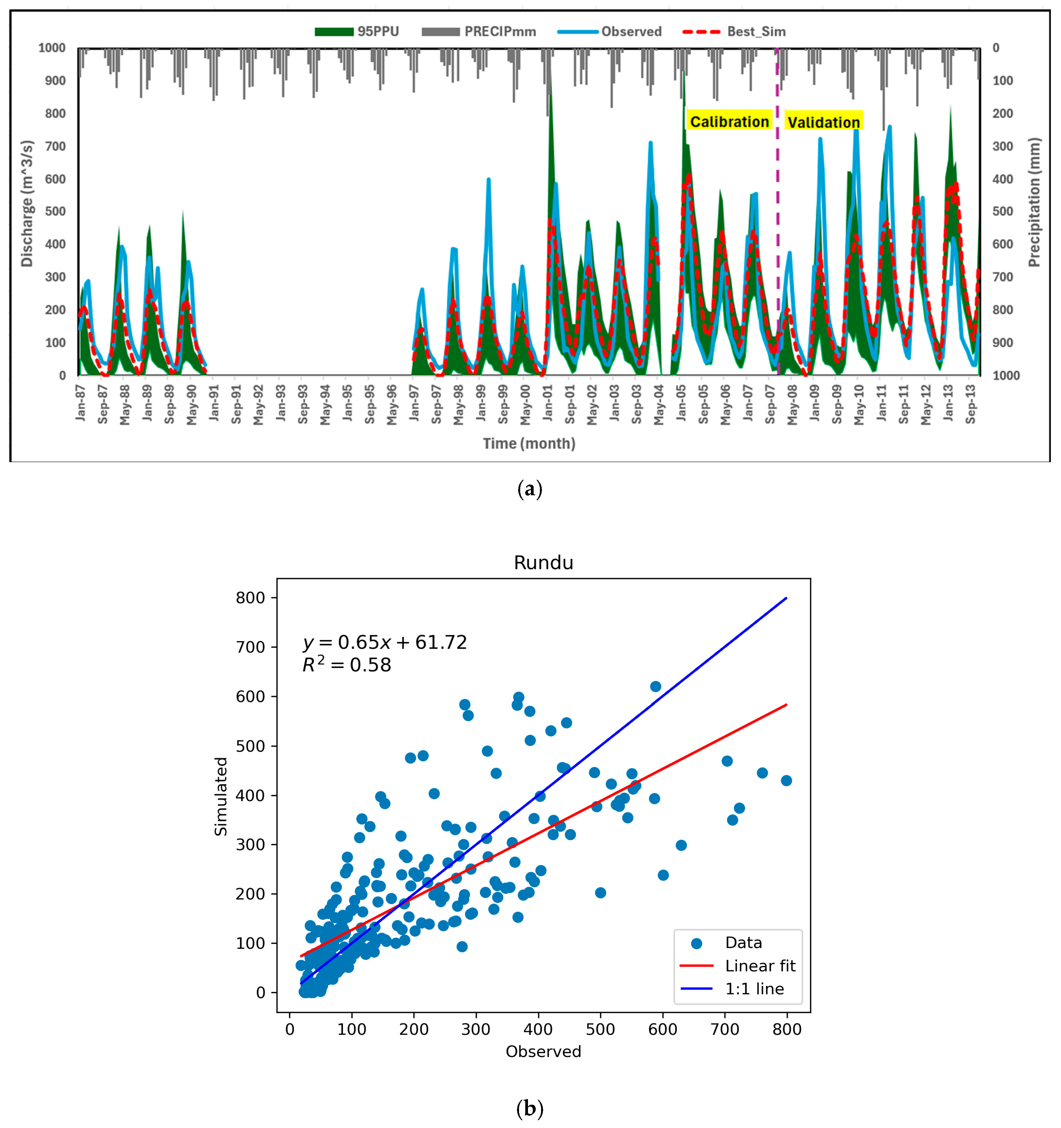
It is important to note that parameter sensitivity may vary over the calibration period and is not consistent across all time steps. Figure 2 illustrates the comparison between observed and simulated streamflow at the Rundu station, along with the corresponding linear regression fit and coefficient of determination.

As shown in Figure 2a, streamflow increased over the study period, consistent with the precipitation data. In this figure, the light blue curve is the observed streamflow, the broken (red) curve is the best-simulated streamflow, the dark green shade is the 95PPU, and the dark grey bar graph along the inverted axis is precipitation. From 1987 to 2000, the Rundu station experienced predominantly low flows, with notable gaps in the observational record (November 1990–December 1996 and June–September 2004) (Nov. 1990 to Dec. 1996 and Jun. 2004 to Sep. 2004). The model proved its capability of simulating the low- and high-flow periods, underestimating some peaks from 1997 to 2000 and 2008 to 2011 and slightly overestimating between 1987 and 1990, 2001 and 2007, and 2012 and 2013. The baseflow conditions were generally well simulated, as reflected in the alignment of the simulated and observed curves. The 95PPU enclosed about 66% of the observed streamflow, as indicated in

Table 3. Model efficiency evaluation for calibration and validation periods.

Period	Station Name	Efficiency Coefficients and Statistics					Time Coverage
		p Factor	r Factor	R2	NSE	PBIAS
Calibration	Rundu	0.66	1.22	0.61	0.59	4.4	Jan. 1987–Dec. 2007
	Dirico	0.75	1.25	0.49	0.41	−28.7	Jan. 2003–Dec. 2007
	Cuito	0.29	0.60	0.72	0.64	−6.4	Jan. 2003–Aug. 2007
	Mukwe	0.68	0.76	0.47	0.26	14.5	Jan. 1987–Dec. 2004
	Mohembo	0.73	1.28	0.53	0.19	−0.9	Jan. 1989–Dec. 1996
Validation	Rundu	0.56	0.98	0.51	0.51	0.1	Jan. 2008–Dec. 2013
	Dirico	0.47	0.76	0.69	0.42	36.1	Jan. 2008–Dec. 2010
	Cuito	0.20	0.47	0.55	0.54	19.4	Sep. 2007–Jul. 2010
	Mukwe	0.50	0.54	0.55	0.44	6.4	Jan. 2005–Dec. 2013
	Mohembo	0.77	1.16	0.63	0.34	0.3	Jan. 1997–Dec. 2000

. Figure 2b shows the fitted curve between the observed and best-simulated streamflow together with the 1:1 line, which serves as a benchmark for perfect correlation. The regression line falls below the 1:1 line, indicating a tendency toward slight underestimation. Nevertheless, the model performance is considered satisfactory based on the coefficient of determination of 0.58 (the value >0.5 is acceptable).

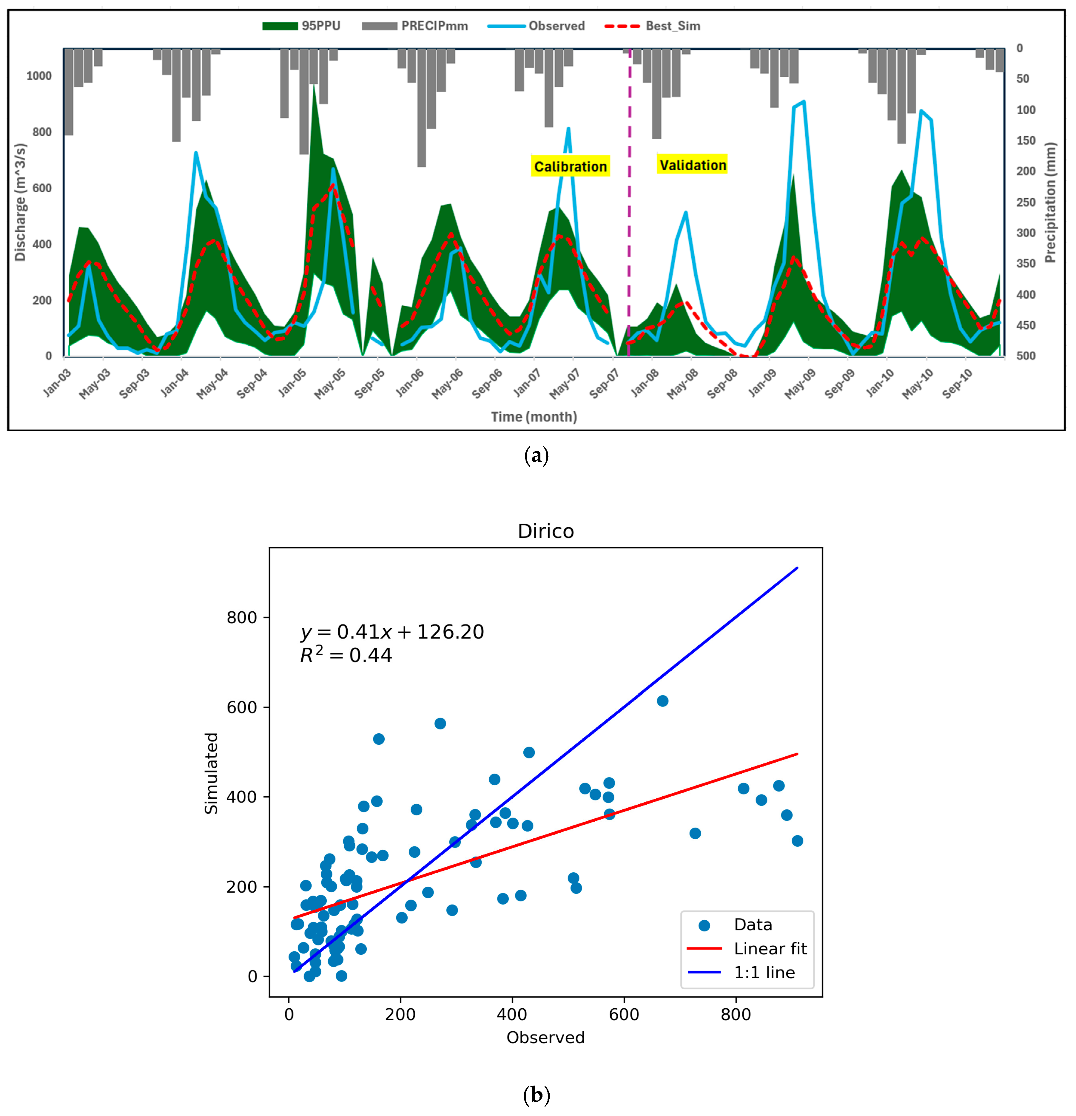
The Dirico station is located in the lower part of the watershed and is hydrologically connected to the upstream Rundu; thus, its simulation is influenced by the calibration results from the upper watershed. The observed monthly data available for this station are smaller than that at the Rundu station, with missing data in Jul. 2005, Oct. 2005, and Sep. 2007. Model performance shows mixed results: peak flows are underestimated between 2008 and 2010, while it is overestimated between 2003 and 2006. As shown in Figure 3a, the 95% 95PPU captures approximately 75% of the observed streamflow, suggesting reasonable model performance despite data limitations. However, the linear regression fit in Figure 3b deviates more significantly from the 1:1 line than at Rundu, indicating a higher degree of bias. Most data points lie above the 1:1 line, implying that the model generally overestimates streamflow at Dirico, making it more biassed compared to the Rundu station.

The Cuito station is located in the eastern branch of the basin. The Cuito station has the shortest data record among the five stations used in the study. Despite the limited data availability, the model performs reasonably well at this site, as evidenced by the performance metrics (R², NSE, and PBIAS) reported in Table 3. However, only 29% of the observed streamflow values fall within the 95% prediction uncertainty (95PPU) interval (Figure 4a). The model overestimated the peaks from 2003 to 2006, while it underestimated the peaks from 2007 to 2010. There is also a shift in peak in 2005 to the left, which might be related to flow resistance in association with the land cover in the upstream area of the sub-basin or bias in recording the observed flow. Additionally, the model overestimated the baseflow as observed in Figure 4a and it underestimated the peak flows in the later years of the record. The coefficient of determination (R² > 0.6) shown in Figure 4b suggests a reasonable correlation between observed and simulated streamflow, and the deviation of the regression line from the 1:1 line is within acceptable limits. This result aligns with the PBIAS value of −6.4 reported in Table 3, where the negative bias confirms a general overestimation of streamflow by the model at this station.

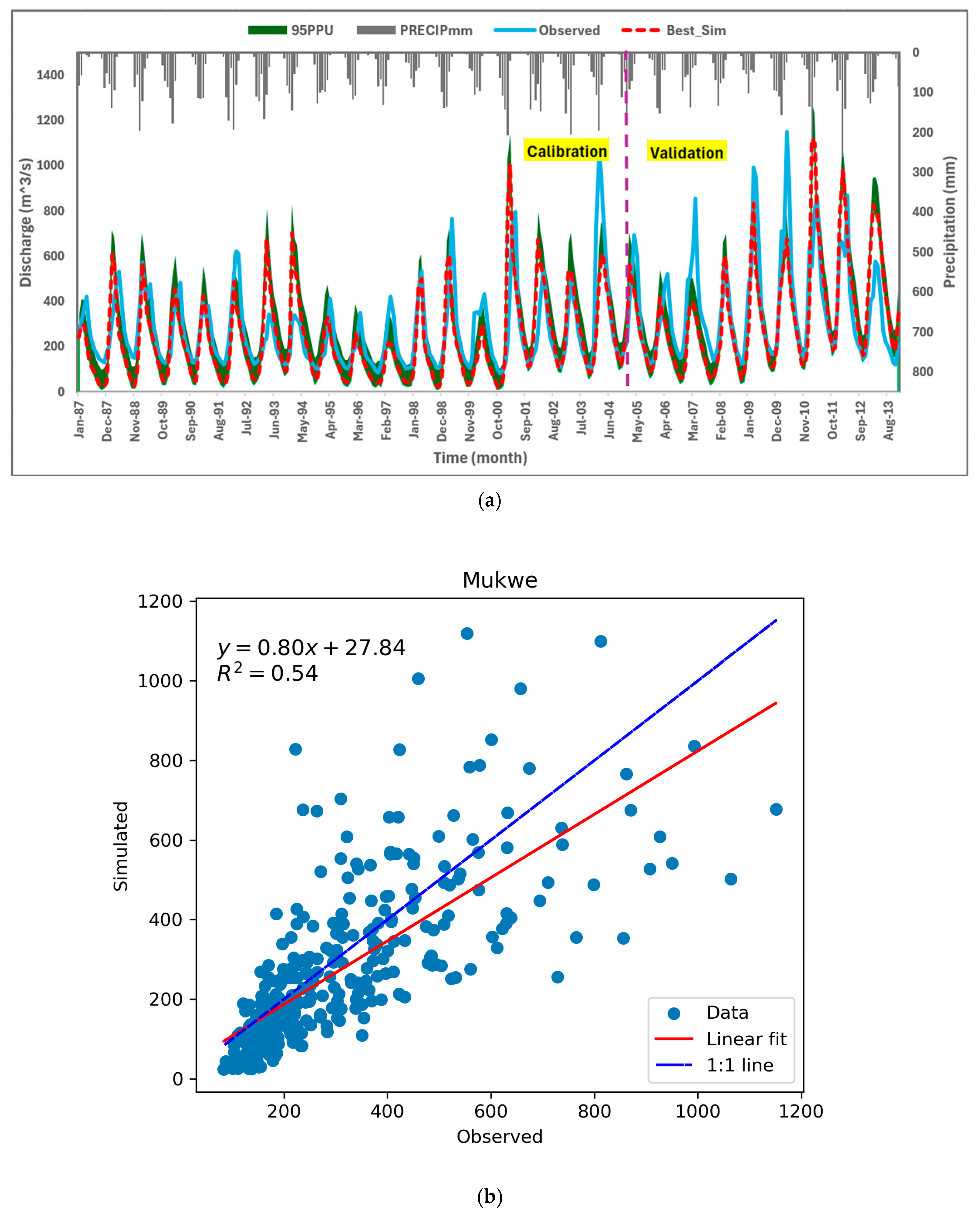
The Mukwe gauge station, located just downstream of the confluence of the two headwaters near Dirico, has the longest uninterrupted monthly discharge record among the five stations, making it ideal for assessing long-term hydrological patterns and the influence of climatic drivers such as ENSO. The discharge rate is the highest due to the contribution of the two headwaters. Despite this, the model slightly underestimates some peak- and low-flow events, although approximately 68% of the observed streamflow falls within the 95PPU range (Figure 5a). The underestimation can be improved with the compromise of the upstream calibration performance in the one-at-a-time multisite calibration process. However, the overall dynamics of streamflow are well simulated with minor shifts to the left and overestimation during 1993–1994, as well as in 2011 and 2013. Periods of low flow, such as 1987, 1995–1996, and 2006, and high flow years like 2000–2001 and 2009–2011 (Figure 5a) in the Southern Africa region (consistent with regional ENSO-linked hydrological variability [44]), are generally well reproduced. Because of the conventional calibration of multisite outlets from upstream to downstream, the calibration processes influence the calibration/validation of this station and might have contributed to the underestimation of the baseflow. The 1:1 line is very close to the best-fit linear regression line, which indicates acceptable percentage bias (PBIAS), which is 14.5 (see Table 3). The fact that most of the simulation data points are below the 1:1 line (Figure 5b) indicates that the model underestimated the observed flow. Discharge values below about 400 m³/s align well with the 1:1 line, while higher discharge values show greater scatter—a trend also observed across other stations (Figure 2, Figure 3, Figure 4, Figure 5 and Figure 6).

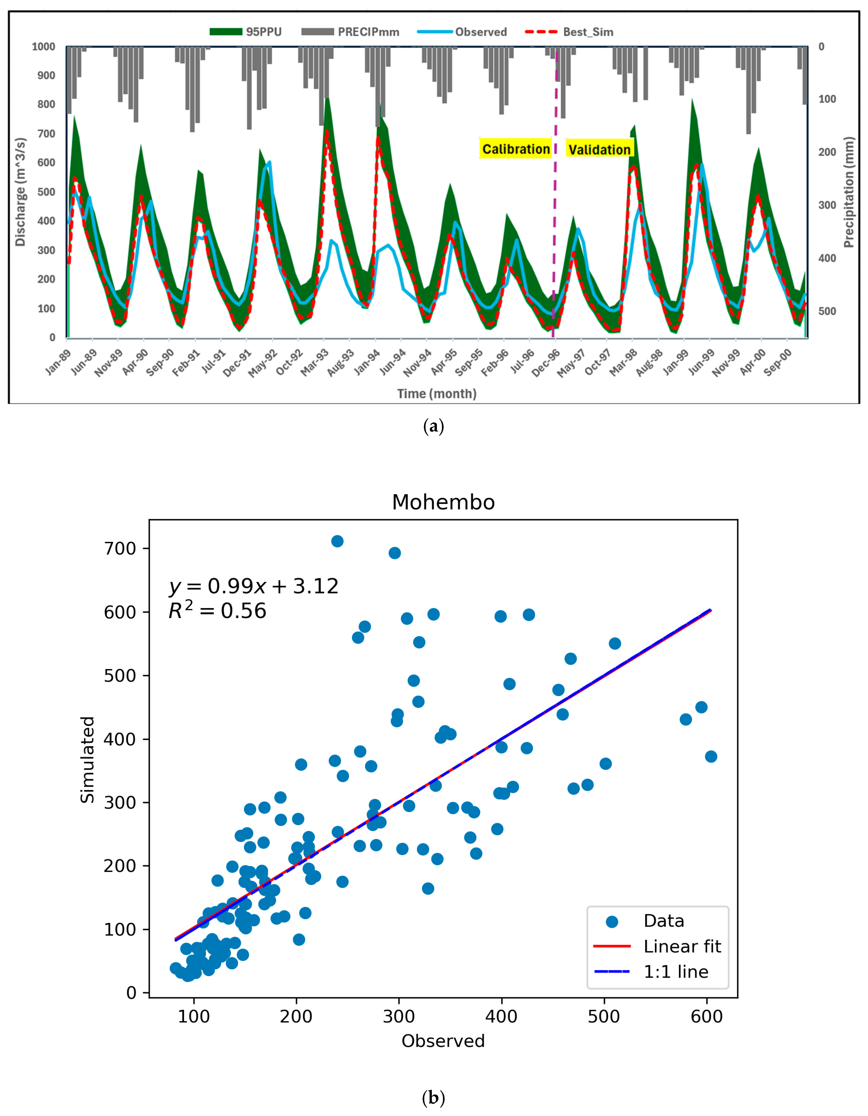
The Mohembo and Mukwe gauge stations are located approximately 40 km apart, with Mohembo situated downstream at the entry point to the Okavango Delta. Being hydrologically connected, Mohembo’s streamflow is directly influenced by upstream calibration, which is evident in the time series plots (Figure 5 and Figure 6). The precipitation at Mohembo is generally lower than at the Mukwe station, resulting in reduced streamflow volumes, particularly during storm events (Figure 6a). Given their close proximity and hydrological connection, many of the patterns observed at Mukwe are also evident at Mohembo, except for notable discrepancies during peak-flow periods in 1993–1994 and 1998, which were significantly overestimated by the model. The model simulated about 73% and 77% of the observed streamflow during calibration and validation periods, respectively, as provided in Table 3, indicating good agreement. The 1:1 line and the linear fit (Figure 6b) are nearly the same, revealing that the PBIAS is minimal, which is −0.9, as shown in Table 3, while the coefficient of determination (R²) is within acceptable limits. Overall, the model slightly overestimated the observed streamflow despite underestimating the low flows.

The SWAT model performance indicators and the temporal coverage for calibration and validation for the Okavango River Basin are summarised in Table 3. These results highlight the hydrological heterogeneity of the basin and the model’s overall capability in simulating streamflow dynamics under varying climatic and spatial conditions. For example, comparing the performance indices for the Cuito station with those of the other stations reveals that, despite a relatively low p-factor, the R², NSE, and PBIAS values are within acceptable thresholds for both calibration and validation periods, based on the criteria established by [45].

In contrast, at the Mukwe and Mohembo stations, the p-factor and r-factor indicate quite a good model uncertainty representation, yet the R², NSE, and PBIAS fall below the satisfactory range. A similar pattern is observed for the Dirico, with the added concern of the highest PBIAS for both calibration and validation periods. These contrasting results underscore the importance of considering a broader set of performance indicators. Hence, according to [33,34,38], we should consider the p-factors and r-factors to represent model performance indices since they provide a more comprehensive evaluation of model performance, as they account for uncertainty and the range of acceptable predictions. In comparison, R², NSE, and PBIAS only measure the degree of agreement between observed and simulated signals, which may not fully capture model behaviour.

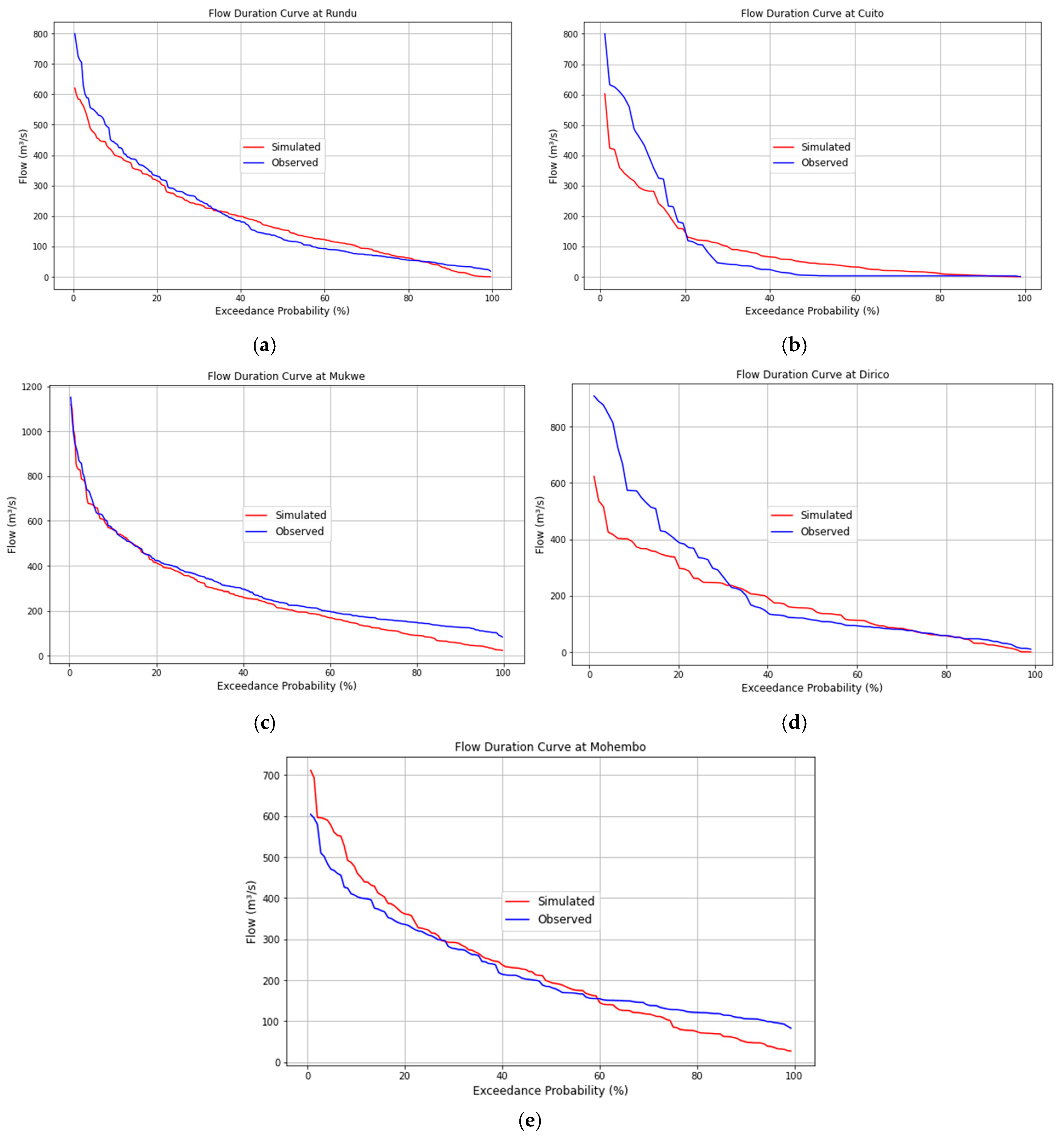
Additionally, the Flow Duration Curves (FDCs) at different sub-watersheds of the basin in Figure 7 offer a graphical summary of streamflow variability. These curves illustrate the percentage of time that streamflow levels are equaled or exceeded over a monthly timescale, providing further insight into the hydrological characteristics of the basin.

The FDCs in Figure 7 represent stations situated in different geographic locations and different geologic formations, providing insights into the hydrological characteristics of the Okavango Basin. Specifically, the Rundu site represents the Cubango branch, the Cutio and Dirico sites represent the Cuito branch, and the Mukwe and Mohembo sites are located downstream after the confluence of the two rivers. The model FDC underestimated the observed extremely high flow in all stations except at the Mukwe (Figure 7), where the simulated FDC closely matches the observed high flows (Figure 7c). At Rundu, the model slightly overestimates the low flows under moderate conditions but underestimates streamflow during the extremely low-flow seasons. At Cuito, the observed FDC indicates periods of almost no discharge (see also Figure 4a), highlighting minimal baseflow, whereas the model slightly overestimates flow for much of the time, though with better agreement in certain periods. The low flow rate is higher at Dirico as compared to the Cuito station, although both Cuito and Dirico belong to the eastern branch of the basin, suggesting increasing contribution from subsurface flow or changes in land cover along the reach. At Mukwe and Mohembo, the model underestimates observed streamflow during the extremely low-flow periods. This result also indicates that while the Cuito branch contributes minimal baseflow at its headwaters, it eventually delivers significant discharge downstream. At Mukwe, the modelled FDC underestimated the observation for the extremely low-flow season.

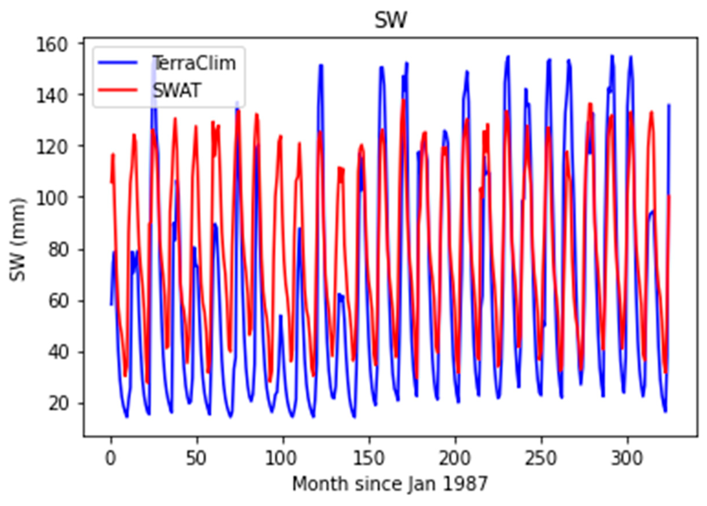
In addition to streamflow, the SWAT model simulation provides several outputs including sediment loads, soil moisture (SW), and evapotranspiration (ET). Some authors (e.g., [46]) have reported the performance of SWAT in reproducing the observed soil water content (SW) and evapotranspiration (ET) when there is a streamflow data shortage to calibrate/validate the model. Figure 8 shows SW from calibrated SWAT and the TerraClimate blended data, offering further validation of the model’s performance across hydrological components.

The coefficient of determination (R²) for SW is 0.63. The SWAT model slightly overestimated observed dry season and wet season soil moisture values, particularly in the earlier periods. Despite this, the calibrated SWAT model may also be used for quick estimates of the soil water moisture content, especially in regions with limited observational data.

3.3. Water Balance of the Okavango River Basin

Water balance simulations help identify and understand key hydrological processes within the catchment, including surface runoff generation, ground–surface water interactions, soil moisture dynamics, and streamflow routing [47]. By simulating these processes, hydrologists can gain insights into the mechanisms driving watershed hydrology and the factors influencing water availability and quality. In this study, WB components are analysed across different regions of the basin, each characterised by distinct soil types, and presented on both annual and interannual timescales. We divided the basin into five parts based on the dominant soil classification. The northwestern part of the basin is dominated by Xanthic Ferralsols (Fx), the northeastern part by Feralic Arenosols (Qf), the middle-left part by Feralic Luvisol (Lf), the middle-right part by Cambic Arenosols (Qc) and the lower part is dominated by Albic Arenosols (Qa) and Eutric Fluvisols (Je) (see Figure 1c for the different soil patches in the basin). These regions correspond to sub-basins 1, 4, 17, 27, and 31, respectively, as shown in Figure 1d. The interannual variability of the WB components for these regions is illustrated in the bar graphs presented in Figure 9.

The precipitation component of the WB decreases progressively from the upstream to the downstream regions, which aligns with the expected climatic gradient in the basin. The sum of the WB components follows a similar trend. Evapotranspiration (ET) is highest in the middle part of the basin (Figure 9c,d), particularly in regions underlain by Ferric Luvisol (Lf) and Cambic Arenosols (Qc)), and is lower in the upper (Figure 9a,b) and the lower (Figure 9e) parts of the basin. Soil moisture content (SW) decreases steadily from upstream to downstream changing from about 1800 mm in the northwestern branch subcatchments (Figure 9a) to less than 100 mm in the lower part of the basin in the panhandle area of the Okavango Delta (Figure 9e). Soil moisture storage (ΔSW), however, does not follow this pattern. The movement of water into the underground aquifer (percolation) is lowest in the central regions (Figure 9c,d)), where soils are characterised by Ferric Luvisol and Cambic Arenosols, and is generally below 180 mm across the transect from the left to right edges of the basin. In contrast, higher percolation rates are observed in the upper (Figure 9a,b) and lower (Figure 9e) parts of the basin, reaching 900 mm in the northwest regions (Figure 9a) and 400 mm in the lower (panhandle) region (Figure 9e) of the basin. The surface runoff is highest in the northwestern regions dominated by Ferralsols soil (Figure 9a), which reaches above 450 mm, while in other regions with different soil types, this component is quite low below 200 mm. The subsurface runoff similarly reaches its minimum in the central part of the basin (Figure 9c–d) covered by Ferric Luvisol and Cambic Arenosols.

The lateral flow component contributes a very small portion to the total water balance in the basin, with values ranging from 0 to 14 mm, peaking in the upper basin and reaching the lowest levels downstream. As observed from Figure 9, evapotranspiration is the major mechanism for removing water from the basin. The basin average evapotranspiration to precipitation ratio in this model is about 64%, but this value is expected to increase up to 95% in the lower part of the basin, consistent with previous studies [18]. Model prediction of water balance components is crucial as their measurement is difficult [48]. It would be more complicated for large river basins, but it helps to quantify freshwater (blue and green) resources.

The other important WB component (not included in the water balance fluxes mentioned above) is water yield (WYLD), which represents the total volume of water generated from a specific area. In the northwest region, WYLD varies between 200 and 1300 mm, while in the northeast region, it ranges from 200 to 730 mm. In the middle part of the basin, this component is the lowest as compared to other regions, with water yield ranging from 0 to 233 mm, which indicates that the tributaries in this area might be ephemeral. In the lower basin, this component ranges from 72 to 333 mm, exceeding those in the central region.

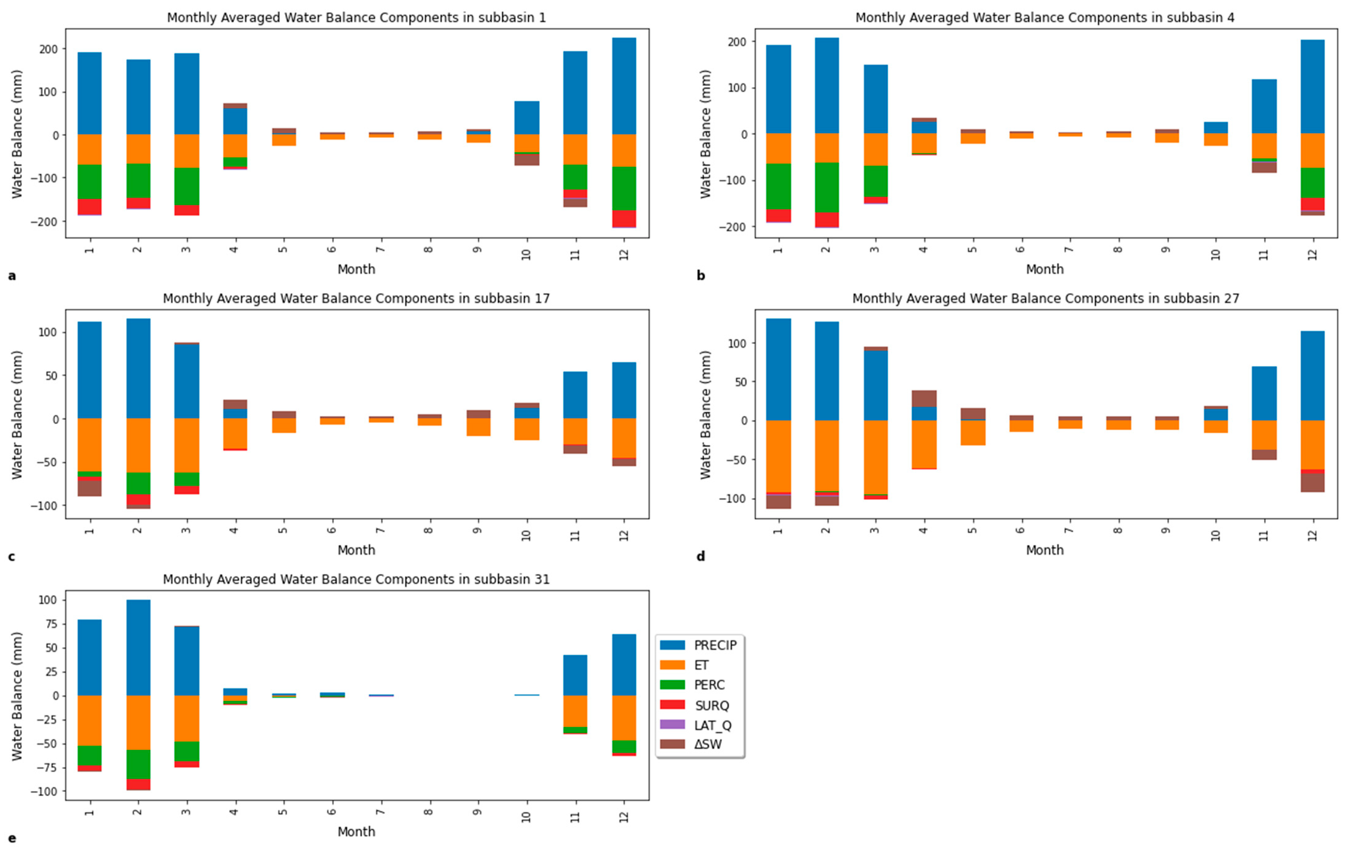
The seasonal cycle of WB components from January to December, obtained by taking the average over the entire years of simulation for each month, is shown in Figure 10. This seasonal analysis provides further insight into the spatio-temporal variability of hydrological responses across subregions dominated by distinct soil types.

The total water balance components exhibit a marked decrease from upstream to downstream regions, as illustrated in Figure 10a–e. This spatial trend closely follows the regional precipitation gradient, where rainfall intensity declines southward. ET tends to increase from the northern to southern parts of the catchment, but this pattern is pronounced primarily during the rainy season (November of the previous year to March of the following year), likely driven by elevated temperatures and vegetation activity in the lower basin.

Soil water content (SW) shows a consistent downstream decline, reflecting the cumulative effect of reduced precipitation and increased ET. In contrast, the soil water storage (ΔSW) is higher in the central region of the basin than in the upstream and downstream areas, suggesting a temporary accumulation or buffering capacity in these zones. However, the percolated amount of water from the soil profile to the shallow aquifer (PERC) is lowest in the central basin (Figure 10c,d) compared to the upstream (Figure 10a,b) and downstream (Figure 10e) of the basin. The central basin is dominantly covered by Ferric Luvisols and Humic Podzols—which typically have finer textures (e.g., silty clay) and lower hydraulic conductivities, thereby impeding vertical water movement and limiting groundwater recharge.

4. Discussion

4.1. Parameter Sensitivity of ORB

The ORB is one of the largest basins in Southern Africa and is characterised by its heterogeneities in climate, geology, topography, and pedology, as well as a scarcity of hydrometeorological data, which poses challenges in the hydrological modelling of the basin. A rigorous sensitivity and calibration analysis was conducted, following a thorough assessment of the quality of observed runoff data to ensure the reliability and accuracy of hydrological simulations. This included visual inspection, assessment of metadata and documentation, examination of data continuity, and evaluation of quality control flags.

The sensitivity analysis, summarised in Table 2, elucidates the differences in the basin’s hydrological responses across the five gauging stations, as observed from the different fitted parameter values. The sensitivity and significance of the parameters were determined by the p-value and t-stat, where parameters with p < 0.05 and high t-stat values were deemed most influential [35,38]. The most sensitive parameters identified in the basin from the initial sensitivity analysis in this manner are ESCO, CN2, SOL_K, and SOL_BD, all of which exhibited significant variation from one station to another. The dominant sensitive parameters are mainly from the soil and management categories, reflecting the spatial heterogeneity of the basin. For instance, the peculiar characteristics of the Cuito sub-basin are well captured through the significant influence of parameters such as SOL_K, SOL_BD, SOL_Z, GWQMN, GW_DELAY, and REVAPMN. Additional influential parameters across the basin include SOL_AWC and ALPHA_BF, highlighting the role of both soil properties and groundwater processes in streamflow dynamics. Most of the parameters listed in Table 2 are consistent with those reported in previous works focused on the ORB and surrounding basins [14,40,41]. Some of the parameters with p-values > 0.05 were retained for calibration based on model performance needs.

Calibrating the model using streamflow data from multiple gauging stations can provide insights into spatially variable watershed responses to hydrological drivers. This multisite calibration approach enhances the representativeness of the model across the basin and improves the accuracy and reliability of hydrological predictions as suggested by [17]. Different studies applying similar techniques in other parts of the world also support this approach [10,46,49].

4.2. Calibration/Validation and Time Series of Streamflow

The simulation results (Figure 2, Figure 3, Figure 4, Figure 5 and Figure 6) indicate quite satisfactory alignment between observed and simulated monthly streamflow across both high- and low-flow periods, suggesting the model’s suitability for predicting average monthly streamflow for such a large, data-scarce, heterogenous watershed. The performance statistics, specifically the p-factor (>0.7) and r-factor (<1.5), fall within acceptable ranges for monthly discharge simulations in basins of comparable size and complexity [34,35] and the values may vary depending on the complexity of the watershed [38]. Such variation is clearly observed in sub-watersheds located further downstream. Furthermore, statistical assessments show a positive correlation between observed and simulated monthly river discharge. Calibration and validation results at multiple stations further substantiate model credibility. Evaluation metrics—including the R², NSE, and PBIAS—fall within or exceed the acceptable thresholds recommended for hydrologic models by Moriasi et al. [45,50], with most stations showing NSE > 0.5 and PBIAS within ±25%. This supports previous findings in similarly semi-arid African basins where SWAT has been shown to effectively simulate seasonal hydrological variability, despite limited ground-based data [51,52].

The basin heterogeneity can be revealed from these results, and the SWAT rainfall-runoff model has satisfactorily captured the hydrological processes across the different sub-basins. One of the advantages of using a multisite calibration technique for large watersheds like the ORB could be its consideration of basin heterogeneities as the parameters are fitted to different values in one-at-a-time calibration for different outlets at different sub-basins. This approach has been widely advocated in large, complex basins (e.g., Nile, Niger, Limpopo), where single-site calibration tends to oversimplify the spatial dynamics of streamflow [53,54,55,56]. Put differently, a calibration conducted at a single site typically pertains to the outlet of the watershed, where all parameters are indicative of the average conditions across the entire region [10,11,12,54].

However, the disadvantage of multisite calibration for rivers in the same network could be that it may pose difficulty to calibrate outlets downstream after calibrating the upstream ones. Parameters calibrated for upstream stations can constrain the flexibility of downstream calibration due to flow routing and mass balance continuity within the model. This is observed in our calibration of ORB, which led to the underestimation of low flows at Mukwe and Mohembo stations, located downstream of the previously calibrated upstream station. Similar effects have been reported by [57,58], where constrained upstream calibration led to sub-optimal downstream simulations, particularly in nested river networks. Some authors even prefer single-site calibration over multisite, not only for its simplicity but also because they report that it has not improved the calibration [59], while others argue that there are pros and cons of single-site and multisite calibrations [8].

Based on our observations of the streamflow time series in Figure 2, Figure 3, Figure 4, Figure 5 and Figure 6, it is evident that the model underestimates the observed low flows at the Mukwe and Mohembo stations. This could be not only due to parameter constriction in the upstream but also due to the underestimation of rainfall, and limited information on point sources and aquifer properties. These two stations were calibrated following the upstream stations, where the variables are constrained to optimise the streamflow there. Parameters constrained in the upstream sub-watersheds during calibration can influence the downstream sub-watersheds for calibration in integrated hydrological models because of the spatial transferability of hydrological model parameters across different scales within a watershed [60,61,62]. For example, parameters related to soil infiltration rates, land cover characteristics, or channel routing in the upstream sub-watershed can influence the timing and magnitude of flows reaching the downstream sub-watershed. Likewise, parameters related to groundwater storage and baseflow generation in the upstream sub-watershed can influence the baseflow contribution to a discharge at the downstream area, and changes in these parameters can alter the timing and magnitude of baseflow entering the downstream sub-watershed, which, in turn, affects its hydrological characteristics. As noted by [63,64], accurate simulation of low flows in semi-arid regions depends heavily on properly representing groundwater–surface water interactions and understanding aquifer dynamics. In the ORB, this is particularly important for the Cuito and Cubango tributaries, where groundwater contributions are suspected to maintain dry-season flows downstream into the Okavango Delta [25,65]. Furthermore, the limited representation of point sources, spatially varying rainfall inputs, and groundwater characteristics in the model may contribute to the observed biases. As stated in previous studies [66], incorporating spatially refined inputs—particularly high-resolution precipitation datasets and detailed hydrogeological information—significantly improves model performance in hydrologically complex and data-scarce regions.

The Cubango and Cuito branches of the ORB exhibit distinct geomorphological and hydrological characteristics that influence water availability and flow regimes downstream. The Cubango branch exhibits a distinct profile, featuring deeply carved channels with relatively narrow widths, showcasing V-shaped valleys and displaying variability in flow rates across seasons. In contrast, the Cuito branch of the Okavango River is characterised by broad, flat-bottomed floodplain valleys that provide ample opportunities for groundwater recharge through infiltration into the soil and replenish groundwater reserves, which, in turn, contributes to baseflows sustaining streamflow downstream during dry periods when the Cubango level is low [27,28]. The Cuito features thick, permeable Kalahari sands overlaid by well-drained Arenosols (see Figure 1c for a soil map of the Basin).

The Cubango catchment is primarily composed of weathered basement crystalline and metamorphic rocks overlain by Ferralsols, which limit infiltration and enhance surface runoff. Conversely, the highly permeable Kalahari sands in the Cuito region promote minimal surface runoff but substantial infiltration, resulting in significant groundwater recharge and extensive groundwater storage [27,28]. The fitted parameter values for the Cuito station in Table 2 are in line with these concepts with the highest saturated hydraulic conductivity (SOL_K), the lowest bulk density (SOL_BD), the thickest upper layer of soil (SOL_Z), and the highest threshold depth of water in the shallow aquifer required for return flow to occur (GWQMN). The Arenosols soil class covers a large extent of the basin, and its characteristic of low available water storage capacity and high infiltration rate is documented in other studies of the region [14,28].

Drainage density and storativity further differentiate the two branches. The Cuito branch exhibits lower drainage density and higher storativity than the Cubango, aligning with observed differences in model parameters and flow duration behaviour [14]. The underestimation of the flow in the downstream part of the ORB could also be related to different channel transmission losses in the region because of high evapotranspiration, alluvial aquifers (layers of sediments), human interventions (e.g., channelisation, surface/groundwater extraction for agriculture, industry, domestic use, etc.), geomorphology, drainage density among others [19]. In the neighbouring river basin of Limpopo, channel transmission losses play a significant role, which amounts to nearly 30% of the water balance [67,68]. Another study [69] on the modelling transmission loss process on two dryland catchments (Middle Jaguaribe River in Brazil) and (Walnut Gulch Experimental Watershed in Arizona, USA) demonstrated the importance of developing accurate models to predict water loss in dryland channels considering the complex interactions between surface water, groundwater, and the surrounding environment.

This discussion suggests that further understanding of flows at Mukwe and Mohembo using multisite calibration requires further investigation to identify whether this is related to model calibration issues, sedimentation, channelisation, urbanisation, water abstraction, or climate change, despite its pronounced multiannual and interannual variability [16,18]. Furthermore, considering the large size of the river basin (190,200 km² or 19,020,000 ha), the absence of a point source, along with the lack of water abstraction data for irrigation, basin development adds to the complexity. The usage of global datasets instead of higher resolution local inputs (e.g., soil, land use land cover, and climate data) likely contributes to uncertainties in streamflow simulations across all stations. In addition, limitations in the current modelling framework, such as the absence of groundwater modules in standalone ArcSWAT, restrict the ability to simulate lateral groundwater flow and transmission losses. Integrating groundwater models could enhance the representation of baseflow and aquifer dynamics.

The monthly Flow Duration Curve (FDC) (Figure 7) supports these findings. At the Cuito station, the flat FDC base and minimal variation in peak-to-low flow ratios (2:1) underscore the dominance of baseflow, consistent with thick sandy soils that favour infiltration and groundwater recharge. In contrast, the Cubango’s flow variability reaches a 10:1 ratio during the wet season, indicating strong surface runoff responses [23]. The model underestimates extremely low flows at Mukwe, pointing to potential issues in simulating dry-season baseflows, which are critical for ecological sustainability and drought preparedness [70]. Overall, the FDC of observed and simulated streamflow show good agreement, with more flow dynamics at the Rundu and Mukwe gauge stations. While both are perennial rivers, Cuito shows more sustained flow, playing a key role in maintaining downstream hydrological stability.

The performance of a model in a watershed is commonly assessed by comparing the observed and simulated streamflow. However, in some data-scarce regions, researchers use evapotranspiration [46,71] and soil moisture [72] from remote sensing to calibrate their model outputs. These components are essential for water balance assessment and drought monitoring. As shown in Figure 8, the model captures seasonal SW variation but tends to overestimate values relative to the TerraClimate dataset. Improved simulation of SW and ET enhances model accuracy and provides deeper insights into watershed hydrology.

4.3. Spatio-Temporal Variation in Water Balance Components

The management of water resources requires an understanding of the quantity, quality, and behaviour of the water resource components for optimum utilisation of both surface and groundwater while minimising environmental degradation [48]. The simulation of Water Balance (WB) fluxes by the hydrological model provides valuable insights into watershed hydrodynamics, enabling the assessment of spatio-temporal variability in key hydrological components. The annual and seasonal time series of the water balance components within the soil profile in the basin are shown in Figure 9 and Figure 10. The interannual variation (Figure 9) in the water balance components largely follows the interannual variation in precipitation across the selected regions (sub-basins). For instance, the years 1989, 1992, 1994, 2000, and 2007 are characterised by a relatively lower amount of water balance components for the northwest regions (Figure 9 a), while the year 1996 is the lowest for the northeastern part of the basin (Figure 9 b). Similarly, for the middle western part (Figure 9c), 1987 and 2009, and for the middle eastern part (Figure 9d), the years 1987 and 1996, have the lowest total water balance component values. The southern sub-basin (Figure 9e) also records reduced water balance during 1987, 1996, and 2009. These deficits correspond to periods of reduced rainfall and are linked to major climate anomalies such as El Niño, which is known to suppress rainfall over Southern Africa [73]. In 1987, the region experienced the El Niño phenomenon, as documented in [44], and Figure 9 indicates reduced streamflows in the middle and lower basin, consistent with El Niño’s influence on hydrology.

Conversely, relatively high WB component totals are recorded during wet years. The years 2001, 2005, and 2009–2013 for the northwest (Figure 9a), as well as 1993, 2001, and 2006 for the northeastern part (Figure 9b) of the basin, are associated with relatively higher quantities of the total available water balance components. In the middle western part (Figure 9c), the years 1991–1992, 2000, and 2010–2011 show higher quantities of the total sum of water balance components. Similarly, in the middle eastern part (Figure 9d), the years 1990, 1992, 2001, and 2011–2012 also demonstrate increased quantities of these components. For the lower part of the basin (Figure 9e), the years 1993, 2004, 2006, and 2012 exhibit relatively higher total water balance components. These correspond to La Niña periods (2010–2012), which typically enhance rainfall across the region [44,74], highlighting the sensitivity of the basin to El Niño–Southern Oscillation (ENSO) forcing.

Figure 10 reveals the seasonal variation in water balance. The soil storage value can be positive when it contributes to the discharge to the stream (through lateral flow) during the dry season, while it is negative during wet seasons, which implies a contribution to the aquifer recharge. This is clearly observed in the upper and middle parts of the basin. In this study, annual rainfall (in mm) is estimated to be 1116, 917, 458, 564, and 369, decreasing from the upstream Angolan Highlands to downstream Namibia and Botswana. While CHIRPS data estimate 1200 mm for the Angolan headwaters, FAO in [75] reports national annual averages of 865 mm (Angola), 465 mm (Namibia), and 495 mm (Botswana). This discrepancy suggests that the use of in situ gauge data—where available—could reduce uncertainties in simulated streamflow and associated WB components.

The corresponding evapotranspiration (ET) ratio to precipitation in these sub-basins is estimated as 0.47, 0.49, 0.82, 0.95, and 0.67 showing increment from upstream to downstream, except at sub-basin 31, where it is expected to be highest. Similarly, the water yield (WYLD) ratio is found to be 0.51, 0.48, 0.11, 0.03, and 0.34, respectively. Higher WYLD is simulated in the upstream sub-basins, while the lower values are in the middle sub-basins, particularly in the eastern branch. The lowest WYLD of 0.03 at sub-basin 27 reflects low surface runoff and minimal groundwater discharge throughout much of the year. The groundwater (GW) ratio follows the same pattern as WYLD, with values of 0.34, 0.34, 0.03, 0, and 0.25, respectively. This indicates that the Cuito sub-catchment functions primarily as a recharge zone, sustaining downstream baseflow. The ET and GW ratios for the eastern sub-basin (sub-basin 27 at Cuito station) indicate that the water in this area has a fate of evaporation or infiltration, which ultimately goes to an aquifer recharge. The contribution of an aquifer to baseflow at this station is negligible as the site recorded 0.3 to 7.3 mm discharge for about 50% of the time (see Figure 7b). However, the lateral and return flows to the river from soil storage likely support baseflow in this area. In both Figure 9 and Figure 10, the soil layer storage values alternate between positive and negative, indicating temporal transitions between streamflow and groundwater recharge contributions. This information has implications for the quantification of water fluxes, water assessment, the detection of changes in trend, and the evaluation of management practices because the differences in their hydraulic conductivity can influence how each soil type manages water and its effects on various agricultural and environmental applications. To better capture groundwater–surface water interactions, we recommend coupling the SWAT model with a physically distributed groundwater model. The standalone SWAT framework lacks the capability to simulate groundwater flow based on hydraulic head gradients, limiting its ability to represent lateral aquifer behaviour and transmission losses across complex terrains.

5. Conclusions

This study applied the ArcSWAT model, calibrated using the SWAT-CUP SUFI2 algorithm, to simulate streamflow and assess spatio-temporal variability in water balance components across the transboundary Okavango River Basin (ORB) from 1987 to 2013. Five gauging stations having data within the simulation period (1987 to 2013) were used to address basin heterogeneity in terms of spatio-temporal variation in water balance components and climate variability. The model setup, sensitivity analysis, and calibration processes highlighted the importance of both climatic variability and catchment characteristics in shaping hydrological responses across the basin.

The first four most sensitive parameters identified initially by the SUFI2 program for the basin are ESCO, CN2, SOL_K, and SOL_Z, with sustained variation, particularly in the upper sub-basins. However, in the sensitivity analysis after calibration and validation processes, the SCS curve number under moisture condition II (CN2) and moist bulk density (SOl_BD) are most responsive to changes in hydrology near Rundu and Dirico; upper soil layer depth (SOL_Z) and shallow aquifer required for return flow to occur (GWQMN) are most sensitive around Cuito catchments; and available storage capacity of soil (SOL_AWC) is relatively the most sensitive in the Mukwe and Mohembo area. These spatial trends reflect the basin’s geomorphological and hydrogeological heterogeneity, especially the contrast between the runoff-dominated Cubango and baseflow-driven Cuito sub-catchments.

The multisite calibration of the basin produced overall satisfactory results for calibration with R² values ranging from 0.47 to 0.72; NSE values between 0.19 and 0.64 during calibration. Validation produced R² values of 0.51 to 0.69 and NSE values of 0.34 to 5.4, although challenges remained in accurately capturing peak flows at Rundu and Cuito, and low flows at Mukwe and Mohembo. The magnitude of PBIAS is less than 20, except for Dirico, where a large bias is observed, indicating overestimation for calibration and underestimation for validation periods. These limitations are attributed to upstream parameter constraints, sparse gauge networks, the absence of point source and groundwater abstraction data, and reliance on coarse-resolution assimilated climate datasets, which likely underestimated precipitation in some sub-basins.

Considering the extent of the basin and its data scarcity, the model performance can be regarded as satisfactory as the model captured the heterogeneity of the basin and seasonal dynamics of the streamflow and other water balance components during the simulation period. These results are also reinforced by the Flow Duration Curve for outlets of Cubango and Cuito branches and the downstream part at Mukwe. The results align with the geological features—such as the sandy soils and high storativity of the Cuito, which sustain baseflows during the dry season, versus the flashy runoff behaviour of Cubango.

The ratio of evapotranspiration to precipitation increased downstream, while the ratios of groundwater discharge and water yield to precipitation decreased, indicating the influence of soil texture, topography, and vegetation cover on water partitioning. Variations in rainfall, ET, GW, and SW contribute to the hydrological heterogeneity of the basin, and seasonal changes and climate variability reveal temporal heterogeneity in the water availability of the basin. Temporal trends in water balance components further suggest that ENSO events and interannual rainfall variability significantly affect hydrological patterns in the ORB.

The main challenges and limitations to setting up a model for the transboundary Okavango River Basin and its calibration/validation processes included the limited and uneven distribution of gauging stations for hydrometeorological records, lack of key input datasets (e.g., irrigation, reservoir operations, and aquifer characteristics), and ArcSWAT’s limited capacity to simulate groundwater flows in complex, groundwater-driven systems like the Cuito Basin, together with the inherent conceptual assumptions of the model. The lack of continuous climate data has forced us to use different assimilated datasets, which underestimated the precipitation values in different sub-basins considered in this study. The sequential multisite calibration introduced upstream–downstream parameter constraints, which may have biassed downstream simulations. Attempts to couple SWAT with physically distributed groundwater models were constrained by data unavailability, underscoring the need for more integrated modelling frameworks. SWAT’s limitation to simulate groundwater flow in a physically distributed manner for groundwater-driven catchments of the basin as discussed for the Cuito branch has also contributed to the underestimation of the low-flow season in the lower catchments.

Overall, the multisite-calibrated standalone SWAT has, in general, performed well for estimating available water resources and informing water management strategies in the ORB but needs to be linked to other physically distributed groundwater models to better understand the eastern branch and to some extent the lower parts of the basin. It can also support future impact assessments under climate change and land use transitions. Future efforts should prioritise integration with distributed groundwater models, high-resolution datasets, and improved representation of human activities to better simulate low-flow conditions and enhance water resource planning in this ecologically and socioeconomically critical basin.

References

1. Kumar, P.; Avtar, R.; Dasgupta, R.; Johnson, B.A.; Mukherjee, A.; Ahsan, N.; Nguyen, D.C.H.; Nguyen, H.Q.; Shaw, R.; Mishra, B.K. Socio-hydrology: A key approach for adaptation to water scarcity and achieving human well-being in large riverine islands. Prog. Disaster Sci. 2020, 8, 100134. [Google Scholar] [CrossRef]
2. Mbaiwa, J.E. Causes and possible solutions to water resource conflicts in the Okavango River Basin: The case of Angola, Namibia and Botswana. Phys. Chem. Earth Parts A/B/C 2004, 29, 1319–1326. [Google Scholar] [CrossRef]
3. Brouwer, R.; Bateman, I.J.; Turner, R.K.; Adger, W.N.; Boar, R.; Crooks, S.; Dockerty, T.; Georgiou, S.; Jones, A.; Langford, I.H. Management of a multi-purpose coastal wetland: The Norfolk and Suffolk Broads, England. In Economics of Coastal and Water Resources: Valuing Environmental Functions; Springer: Dordrecht, The Netherlands, 2001; pp. 159–213. [Google Scholar] [CrossRef]
4. Sorooshian, S.; Hsu, K.L.; Coppola, E.; Tomassetti, B.; Verdecchia, M.; Visconti, G. (Eds.) Hydrological Modelling and the Water Cycle: Coupling the Atmospheric and Hydrological Models; Springer Science & Business Media: Berlin/Heidelberg, Germany, 2008. [Google Scholar]
5. Mahmoodi, N.; Kiesel, J.; Wagner, P.D.; Fohrer, N. Integrating water use systems and soil and water conservation measures into a hydrological model of an Iranian Wadi system. J. Arid. Land 2020, 12, 545–560. [Google Scholar] [CrossRef]
6. Boufala, M.; El Hmaidi, A.; Chadli, K.; Essahlaoui, A.; El Ouali, A.; Taia, S. Hydrological modeling of water and soil resources in the basin upstream of the Allal El Fassi dam (Upper Sebou watershed, Morocco). Model. Earth Syst. Environ. 2019, 5, 1163–1177. [Google Scholar] [CrossRef]
7. Wang, H.; Chen, Y. Identifying key hydrological processes in highly urbanized watersheds for flood forecasting with a distributed hydrological model. Water 2019, 11, 1641. [Google Scholar] [CrossRef]
8. Singh, L.; Saravanan, S. Assessing streamflow modeling using single and multi-site calibration approach on Bharathpuzha catchment, India: A case study. Model. Earth Syst. Environ. 2022, 8, 4135–4148. [Google Scholar] [CrossRef]
9. Wang, S.; Zhang, Z.; Sun, G.; Strauss, P.; Guo, J.; Tang, Y.; Yao, A. Multi-site calibration, validation, and sensitivity analysis of the MIKE SHE Model for a large watershed in northern China. Hydrol. Earth Syst. Sci. 2012, 16, 4621–4632. [Google Scholar] [CrossRef]
10. Aragaw, H.M.; Mishra, S.K. Multi-site multi-objective calibration of SWAT model using a large dataset for improved performance in Ethiopia. Arab. J. Geosci. 2022, 15, 320. [Google Scholar] [CrossRef]
11. Leta, O.T.; van Griensven, A.; Bauwens, W. Effect of single and multisite calibration techniques on the parameter estimation, performance, and output of a SWAT model of a spatially heterogeneous catchment. J. Hydrol. Eng. 2017, 22, 05016036. [Google Scholar] [CrossRef]
12. Chiang, L.-C.; Yuan, Y.; Mehaffey, M.; Jackson, M.; Chaubey, I. Assessing SWAT’s performance in the Kaskaskia River watershed as influenced by the number of calibration stations used. Hydrol. Process. 2014, 28, 676–687. [Google Scholar] [CrossRef]
13. Hiroshi, I.; Kazuyoshi, S.; Jun, M.; Harivelo, R.Z.M.; Fernández-Palomino, C.A. Multi-gauge calibration comparison for simulating streamflow across the Major River Basins in Madagascar: SWAT + Toolbox, R-SWAT, and SWAT + Editor Hard calibration. Hydrol. Res. 2024, 55, 412–430. [Google Scholar] [CrossRef]
14. Hughes, D.A.; Andersson, L.; Wilk, J.; Savenije, H.H. Regional calibration of the Pitman model for the Okavango River. J. Hydrol. 2006, 331, 30–42. [Google Scholar] [CrossRef]
15. Andersson, L.; Wilk, J.; Todd, M.C.; Hughes, D.A.; Earle, A.; Kniveton, D.; Layberry, R.; Savenije, H.H. Impact of climate change and development scenarios on flow patterns in the Okavango River. J. Hydrol. 2006, 331, 43–57. [Google Scholar] [CrossRef]
16. Wolski, P.; Savenije, H.; Murray-Hudson, M.; Gumbricht, T. Modelling of the flooding in the Okavango Delta, Botswana, using a hybrid reservoir-GIS model. J. Hydrol. 2006, 331, 58–72. [Google Scholar] [CrossRef]
17. Baumberg, V.; Helmschrot, J.; Steudel, T.; Göhmann, H.; Fischer, C.; Flügel, W.-A. Assessing basin heterogeneities for rainfall–runoff modelling of the Okavango River and its transboundary management. Proc. Int. Assoc. Hydrol. Sci. 2014, 364, 320–325. [Google Scholar] [CrossRef]
18. Kgathi, D.; Kniveton, D.; Ringrose, S.; Turton, A.; Vanderpost, C.; Lundqvist, J.; Seely, M. The Okavango; a river supporting its people, environment and economic development. J. Hydrol. 2006, 331, 3–17. [Google Scholar] [CrossRef]
19. Pinheiro, I.; Gabaake, G.; Heyns, P. Cooperation in the Okavango River Basin: The OKACOM perspective. In Transboundary Rivers, Sovereignty and Development: Hydropolitical Drivers in the Okavango River Basin; Turton, A., Ashton, P., Cloete, E., Eds.; African Water Issues Research Unit (AWIRU): Pretoria, South Africa, 2003; pp. 105–118. [Google Scholar]
20. Turton, A.; Ashton, P.; Cloete, E. An introduction to the hydropolitical drivers in the Okavango River basin. In Transboundary Rivers, Sovereignty and Development: Hydropolitical Drivers in the Okavango River Basin; African Water Issues Research Unit: Pretoria, South Africa, 2003. [Google Scholar]
21. Andersson, L.; Gumbricht, T.; Hughes, D.; Kniveton, D.; Ringrose, S.; Savenije, H.; Todd, M.; Wilk, J.; Wolski, P. Water flow dynamics in the Okavango River Basin and Delta—A prerequisite for the ecosystems of the Delta. Phys. Chem. Earth Parts A/B/C 2003, 28, 1165–1172. [Google Scholar] [CrossRef]
22. Hughes, D.A.; Kingston, D.G.; Todd, M.C. Uncertainty in water resources availability in the Okavango River basin as a result of climate change. Hydrol. Earth Syst. Sci. 2011, 15, 931–941. [Google Scholar] [CrossRef]
23. Wilk, J.; Kniveton, D.; Andersson, L.; Layberry, R.; Todd, M.C.; Hughes, D.; Ringrose, S.; Vanderpost, C. Estimating rainfall and water balance over the Okavango River Basin for hydrological applications. J. Hydrol. 2006, 331, 18–29. [Google Scholar] [CrossRef]
24. The Permanent Okavango River Basin Water Commission. Cubango-Okavango River Basin Transboundary Diagnostic Analysis; OKACOM: Maun, Botswana, 2011. [Google Scholar]
25. Mendelsohn, J.; El Obeid, S. Okavango River: The Flow of a Lifeline; Struik: Cape Town, South Africa, 2004. [Google Scholar]
26. Permanent Okavango River Basin Water Commission. The Permanent Okavango River Basin Water Commission Annual Report 2009; Permanent Okavango River Basin Water Commission: Maun, Botswana, 2009. [Google Scholar]
27. Jones, M.J. The Groundwater Hydrology of the Okavango Basin; OKACOM Okavango River Basin Transboundary Diagnostical Analysis Technical Report; OKAKOM: Gaborone, Botswana, 2010; pp. 1–83. [Google Scholar]
28. Mendelsohn, J.; Martins, A. River Catchments and Development Prospects in South-Eastern Angola. Available online: https://www.researchgate.net/profile/John-Mendelsohn/publication/341652220_South-eastern_Angola_-_A_synthesis_of_information_RAISON_2019/links/5ecd44734585152945144c0e/South-eastern-Angola-A-synthesis-of-information-RAISON-2019.pdf (accessed on 5 June 2024).
29. Beck, H.E.; Wood, E.F.; Pan, M.; Fisher, C.K.; Miralles, D.G.; van Dijk, A.I.J.M.; McVicar, T.R.; Adler, R.F. MSWEP V2 global 3-hourly 0.1 precipitation: Methodology and quantitative assessment. Bull. Am. Meteorol. Soc. 2019, 100, 473–500. [Google Scholar] [CrossRef]
30. Fuka, D.R.; Walter, M.T.; MacAlister, C.; DeGaetano, A.T.; Steenhuis, T.S.; Easton, Z.M. Using the Climate Forecast System Reanalysis as weather input data for watershed models. Hydrol. Process. 2014, 28, 5613–5623. [Google Scholar] [CrossRef]
31. Huntington, J.L.; Hegewisch, K.C.; Daudert, B.; Morton, C.G.; Abatzoglou, J.T.; McEvoy, D.J.; Erickson, T. Climate engine: Cloud computing and visualization of climate and remote sensing data for advanced natural resource monitoring and process understanding. Bull. Am. Meteorol. Soc. 2017, 98, 2397–2410. [Google Scholar] [CrossRef]
32. Soulis, K.X. Soil conservation service curve number (SCS-CN) Method: Current applications, remaining challenges, and future perspectives. Water 2021, 13, 192. [Google Scholar] [CrossRef]
33. Abbaspour, K.C.; Johnson, C.A.; van Genuchten, M.T. Estimating uncertain flow and transport parameters using a sequential uncertainty fitting procedure. Vadose Zone J. 2004, 3, 1340–1352. [Google Scholar] [CrossRef]
34. Abbaspour, K.C.; Yang, J.; Maximov, I.; Siber, R.; Bogner, K.; Mieleitner, J.; Zobrist, J.; Srinivasan, R. Modelling hydrology and water quality in the pre-alpine/alpine Thur watershed using SWAT. J. Hydrol. 2007, 333, 413–430. [Google Scholar] [CrossRef]
35. Arnold, J.G.; Moriasi, D.N.; Gassman, P.W.; Abbaspour, K.C.; White, M.J.; Srinivasan, R.; Santhi, C.; Harmel, R.D.; van Griensven, A.; Van Liew, M.W.; et al. SWAT: Model use, calibration, and validation. Trans. ASABE 2012, 55, 1491–1508. [Google Scholar] [CrossRef]
36. Gassman, P.W.; Sadeghi, A.M.; Srinivasan, R. Applications of the SWAT model special section: Overview and insights. J. Environ. Qual. 2014, 43, 1–8. [Google Scholar] [CrossRef]
37. Muleta, M.K.; Nicklow, J.W. Sensitivity and uncertainty analysis coupled with automatic calibration for a distributed watershed model. J. Hydrol. 2005, 306, 127–145. [Google Scholar] [CrossRef]
38. Abbaspour, K.C.; Rouholahnejad, E.; Vaghefi, S.; Srinivasan, R.; Yang, H.; Kløve, B. A continental-scale hydrology and water quality model for Europe: Calibration and uncertainty of a high-resolution large-scale SWAT model. J. Hydrol. 2015, 524, 733–752. [Google Scholar] [CrossRef]
39. Koltsida, E.; Mamassis, N.; Kallioras, A. Hydrological modeling using the SWAT Model in urban and peri-urban environments: The case of Kifissos experimental sub-basin (Athens, Greece). Hydrol. Earth Syst. Sci. 2023, 27, 917–931. [Google Scholar] [CrossRef]
40. Arsiso, B.K.; Tsidu, G.M. Land use and land cover change modulates hydrological flows and water supply to Gaborone dam catchment, Botswana. Water 2023, 15, 3364. [Google Scholar] [CrossRef]
41. Gizaw, N.K.; Daniel, W.; Nichola, K.; Miguel, V.O.; Eva, C.P.; Martin, K. Evaluating SWAT model for streamflow estimation in the semi-arid Okavango-Omatako catchment, Namibia. Afr. J. Environ. Sci. Technol. 2022, 16, 385–403. [Google Scholar] [CrossRef]
42. Emam, A.R.; Kappas, M.; Fassnacht, S.; Linh, N.H.K. Uncertainty analysis of hydrological modeling in a tropical area using different algorithms. Front. Earth Sci. 2018, 12, 661–671. [Google Scholar] [CrossRef]
43. Abbaspour, K.C.; Faramarzi, M.; Ghasemi, S.S.; Yang, H. Assessing the impact of climate change on water resources in Iran. Water Resour. Res. 2009, 45. [Google Scholar] [CrossRef]
44. Hoell, A.; Gaughan, A.E.; Magadzire, T.; Harrison, L. The modulation of daily Southern Africa precipitation by El niño–southern oscillation across the summertime wet season. J. Clim. 2021, 34, 1115–1134. [Google Scholar] [CrossRef]
45. Moriasi, D.N.; Gitau, M.W.; Pai, N.; Daggupati, P. Hydrologic and water quality models: Performance measures and evaluation criteria. Trans. ASABE 2015, 58, 1763–1785. [Google Scholar] [CrossRef]
46. Odusanya, A.E.; Mehdi, B.; Schürz, C.; Oke, A.O.; Awokola, O.S.; Awomeso, J.A.; Adejuwon, J.O.; Schulz, K. Multi-site calibration and validation of SWAT with satellite-based evapotranspiration in a data-sparse catchment in southwestern Nigeria. Hydrol. Earth Syst. Sci. 2019, 23, 1113–1144. [Google Scholar] [CrossRef]
47. Neitsch, S.L.; Arnold, J.G.; Kiniry, J.R.; Williams, J.R.; King, K.W. Soil and Water Assessment Tool: Theoretical Documentation: Version 2005 [Internet]. January 2005. Available online: https://swat.tamu.edu/media/1292/swat2005theory.pdf (accessed on 8 May 2024).
48. Nasiri, S.; Ansari, H.; Ziaei, A.N. Simulation of water balance equation components using SWAT model in Samalqan Watershed (Iran). Arab. J. Geosci. 2020, 13, 421. [Google Scholar] [CrossRef]
49. Gowda, A.N.; Patil, N.S. Multisite calibration of the ghataprabha sub-basin using soil and water assessment tool. In Hydrological Modeling: Hydraulics, Water Resources and Coastal Engineering; Springer International Publishing: Cham, Switzerland, 2022; pp. 139–163. [Google Scholar] [CrossRef]
50. Moriasi, D.N.; Arnold, J.G.; van Liew, M.W.; Bingner, R.L.; Harmel, R.D.; Veith, T.L. Model evaluation guidelines for systematic quantification of accuracy in watershed simulations. Trans. ASABE 2007, 50, 885–900. [Google Scholar] [CrossRef]
51. Schuol, J.; Abbaspour, K.C.; Yang, H.; Srinivasan, R.; Zehnder, A.J.B. Modeling blue and green water availability in Africa. Water Resour. Res. 2008, 44, 212–221. [Google Scholar] [CrossRef]
52. Mango, L.M.; Melesse, A.M.; McClain, M.E.; Gann, D.; Setegn, S.G. Land use and climate change impacts on the hydrology of the upper Mara River Basin, Kenya: Results of a modeling study to support better resource management. Hydrol. Earth Syst. Sci. 2011, 15, 2245–2258. [Google Scholar] [CrossRef]
53. Hasan, M.A.; Pradhanang, S.M. Estimation of flow regime for a spatially varied Himalayan watershed using improved multi-site calibration of the Soil and Water Assessment Tool (SWAT) model. Environ. Earth Sci. 2017, 76, 787. [Google Scholar] [CrossRef]
54. Daggupati, P.; Pai, N.; Ale, S.; Douglas-Mankin, K.R.; Zeckoski, R.W.; Jeong, J.; Parajuli, P.B.; Saraswat, D.; Youssef, M.A. A recommended calibration and validation strategy for hydrologic and water quality models. Trans. ASABE 2015, 58, 1705–1719. [Google Scholar] [CrossRef]
55. Song, Y.; Zhang, J.; Lai, Y. Influence of multisite calibration on streamflow estimation based on the hydrological model with CMADS inputs. J. Water Clim. Chang. 2021, 12, 3264–3281. [Google Scholar] [CrossRef]
56. Van Griensven, A.; Ndomba, P.; Yalew, S.; Kilonzo, F. Critical review of SWAT applications in the upper Nile basin countries. Hydrol. Earth Syst. Sci. 2012, 16, 3371–3381. [Google Scholar] [CrossRef]
57. Rouholahnejad, E.; Abbaspour, K.; Vejdani, M.; Srinivasan, R.; Schulin, R.; Lehmann, A. A parallelization framework for calibration of hydrological models. Environ. Model. Softw. 2012, 31, 28–36. [Google Scholar] [CrossRef]
58. Krysanova, V.; Hattermann, F.; Wechsung, F. Implications of complexity and uncertainty for integrated modelling and impact assessment in river basins. Environ. Model. Softw. 2007, 22, 701–709. [Google Scholar] [CrossRef]
59. Franco, A.C.L.; de Oliveira, D.Y.; Bonumá, N.B. Comparison of single-site, multi-site and multi-variable SWAT calibration strategies. Hydrol. Sci. J. 2020, 65, 2376–2389. [Google Scholar] [CrossRef]
60. Sakthivadivel, R.; Scott, C.A. Upstream-downstream complementarities and tradeoffs: Opportunities and constraints in water-shed development in water scarce regions. In Watershed Management Challenges; Government of India: New Delhi, India, 2005; p. 173. [Google Scholar]
61. Roth, V.; Nigussie, T.K.; Lemann, T. Model parameter transfer for streamflow and sediment loss prediction with SWAT in a tropical watershed. Environ. Earth Sci. 2016, 75, 1321. [Google Scholar] [CrossRef]
62. McDonnell, J.J.; Sivapalan, M.; Vaché, K.; Dunn, S.; Grant, G.; Haggerty, R.; Hinz, C.; Hooper, R.; Kirchner, J.; Roderick, M.L.; et al. Moving beyond heterogeneity and process complexity: A new vision for watershed hydrology. Water Resour. Res. 2007, 43, W07301. [Google Scholar] [CrossRef]
63. Masih, I.; Maskey, S.; Uhlenbrook, S.; Smakhtin, V. Assessing the impact of areal precipitation input on streamflow simulations using the SWAT Model 1. JAWRA J. Am. Water Resour. Assoc. 2010, 47, 179–195. [Google Scholar] [CrossRef]
64. Kim, N.W.; Chung, I.M.; Won, Y.S.; Arnold, J.G. Development and application of the integrated SWAT–MODFLOW model. J. Hydrol. 2008, 356, 1–16. [Google Scholar] [CrossRef]
65. Bauer, P.; Gumbricht, T.; Kinzelbach, W. A regional coupled surface water/groundwater model of the Okavango Delta, Botswana. Water Resour. Res. 2006, 42. [Google Scholar] [CrossRef]
66. Bekele, E.G.; Nicklow, J.W. Multi-objective automatic calibration of SWAT using NSGA-II. J. Hydrol. 2007, 341, 165–176. [Google Scholar] [CrossRef]
67. Mvandaba, V.; Hughes, D.; Kapangaziwiri, E.; Kahinda, J.-M.M.; Oosthuizen, N. Modelling of channel transmission loss processes in semi-arid catchments of southern Africa using the Pitman Model. Proc. Int. Assoc. Hydrol. Sci. 2018, 378, 17–22. [Google Scholar] [CrossRef]
68. Mvandaba, V.; Hughes, D.; Kapangaziwiri, E.; Kahinda, J.M.; Hobbs, P.; Madonsela, S.; Oosthuizen, N. The delineation of alluvial aquifers towards a better understanding of channel transmission losses in the Limpopo River Basin. Phys. Chem. Earth Parts A/B/C 2018, 108, 60–73. [Google Scholar] [CrossRef]
69. Costa, A.C.; Bronstert, A.; de Araújo, J.C. A channel transmission losses model for different dryland rivers. Hydrol. Earth Syst. Sci. 2012, 16, 1111–1135. [Google Scholar] [CrossRef]
70. Choi, B.; Kang, H.; Lee, W.H. Baseflow contribution to streamflow and aquatic habitats using physical habitat simulations. Water 2018, 10, 1304. [Google Scholar] [CrossRef]
71. Odusanya, A.E.; Schulz, K.; Biao, E.I.; Degan, B.A.; Mehdi-Schulz, B. Evaluating the performance of streamflow simulated by an eco-hydrological model calibrated and validated with global land surface actual evapotranspiration from remote sensing at a catchment scale in West Africa. J. Hydrol. Reg. Stud. 2021, 37, 100893. [Google Scholar] [CrossRef]
72. Rajib, M.A.; Merwade, V.; Yu, Z. Multi-objective calibration of a hydrologic model using spatially distributed remotely sensed/in-situ soil moisture. J. Hydrol. 2016, 536, 192–207. [Google Scholar] [CrossRef]
73. Hoell, A.; Funk, C.; Zinke, J.; Harrison, L. Modulation of the Southern Africa precipitation response to the El Niño Southern Oscillation by the subtropical Indian Ocean Dipole. Clim. Dyn. 2017, 48, 2529–2540. [Google Scholar] [CrossRef]
74. Shikwambana, L.; Xongo, K.; Mashalane, M.; Mhangara, P. Climatic and vegetation response patterns over South Africa during the 2010/2011 and 2015/2016 strong ENSO phases. Atmosphere 2023, 14, 416. [Google Scholar] [CrossRef]
75. Food and Agriculture Organization of the United Nations (FAO). Irrigation Potential in Africa: A Basin Approach. 1997. Available online: https://openknowledge.fao.org/server/api/core/bitstreams/502d1a57-49d7-4acc-bfdb-6efdfb11a3da/content/w4347e0p.htm (accessed on 6 January 2025).
Figure 1. (a) Delineated study area and DEM (b) LULC (c) Soil classification and (d) The location of Sub-basin labeled from 1 to 31 in the ORB.
Water 17 01442 g001
Figure 2. Calibration and validation of SWAT-simulated streamflow against observation at Rundu: (a) time series comparison of observed and simulated streamflow, and (b) scatter plot with linear regression fit.
Water 17 01442 g002
Figure 3. The same as Figure 2, but for Dirico.
Water 17 01442 g003
Figure 4. The same as Figure 2, but for Cuito.
Water 17 01442 g004
Figure 5. The same as Figure 2, but for Mukwe.
Water 17 01442 g005
Figure 6. The same as Figure 2, but for Mohembo.
Water 17 01442 g006
Figure 7. Flow Duration Curves comparing observed and simulated streamflow at five gauging stations: (a) Rundu, (b) Cuito, (c) Mukwe, (d) Dirico, and (e) Mohembo.
Water 17 01442 g007
Figure 8. Basin average soil moisture (SW) from calibrated SWAT model and TerraClimate dataset.
Water 17 01442 g008
Figure 9. Interannual water balance components in the upper Cubango (a), upper Cuito (b), middle Cubango (c), middle Cuito (d), and Okavango River after the confluence of the two branches (e).
Water 17 01442 g009
Figure 10. Annual cycle of water balance components in the upper Cubango (a), upper Cuito (b), middle Cubango (c), middle Cuito (d), and Okavango River after the confluence of the two branches (e).
Water 17 01442 g010