


Time-Lag Effects of Winter Arctic Sea Ice on Subsequent Spring Precipitation Variability over China and Its Possible Mechanisms


Abstract
1. Introduction
2. Datasets and Methods
2.1. List of Abbreviations
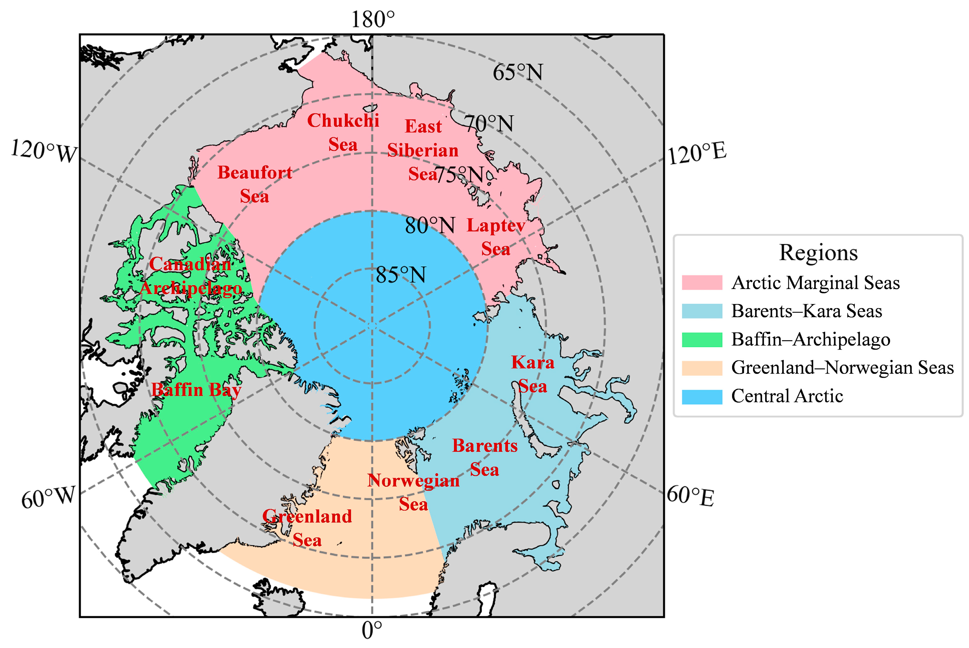
2.2. Study Area
2.3. Datasets
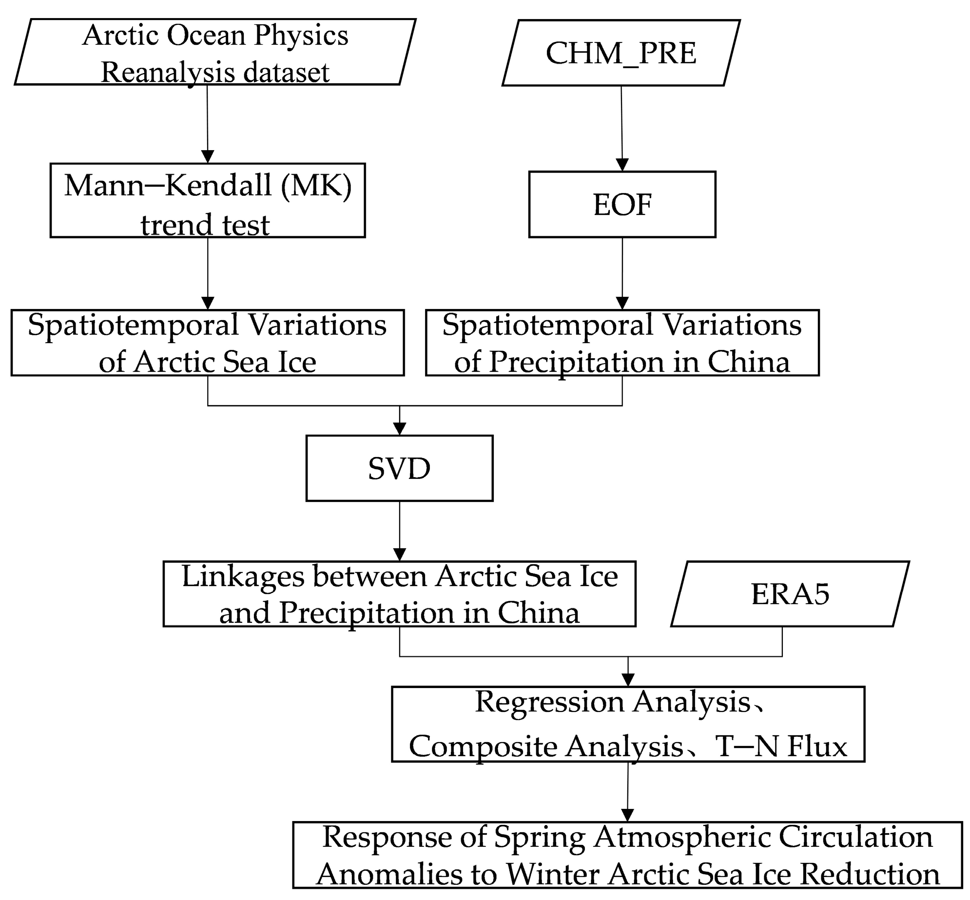
2.4. Methods
2.4.1. Empirical Orthogonal Function (EOF)
2.4.2. Singular Value Decomposition (SVD)
2.4.3. T–N Three-Dimensional Wave-Activity Flux
2.4.4. Multi-Wavelet Coherence (MWC)
2.4.5. Mann–Kendall (MK) Trend Test
3. Results
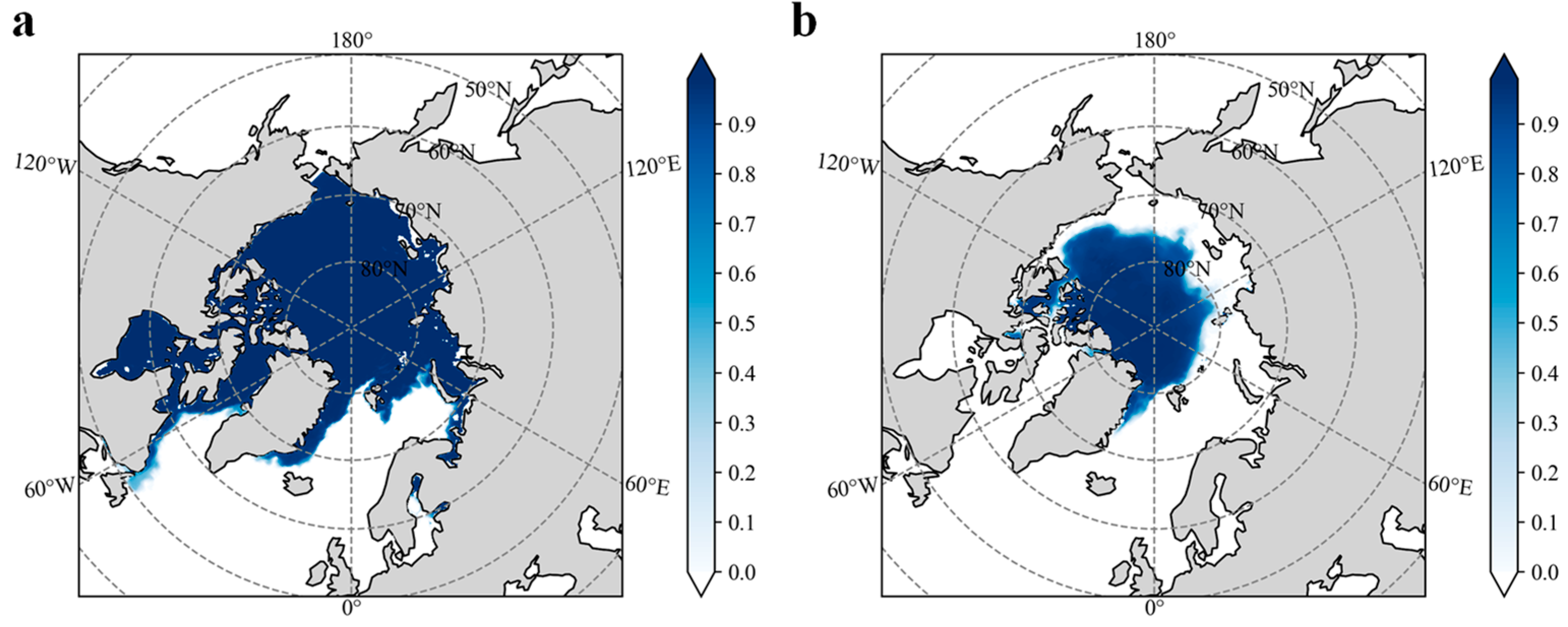
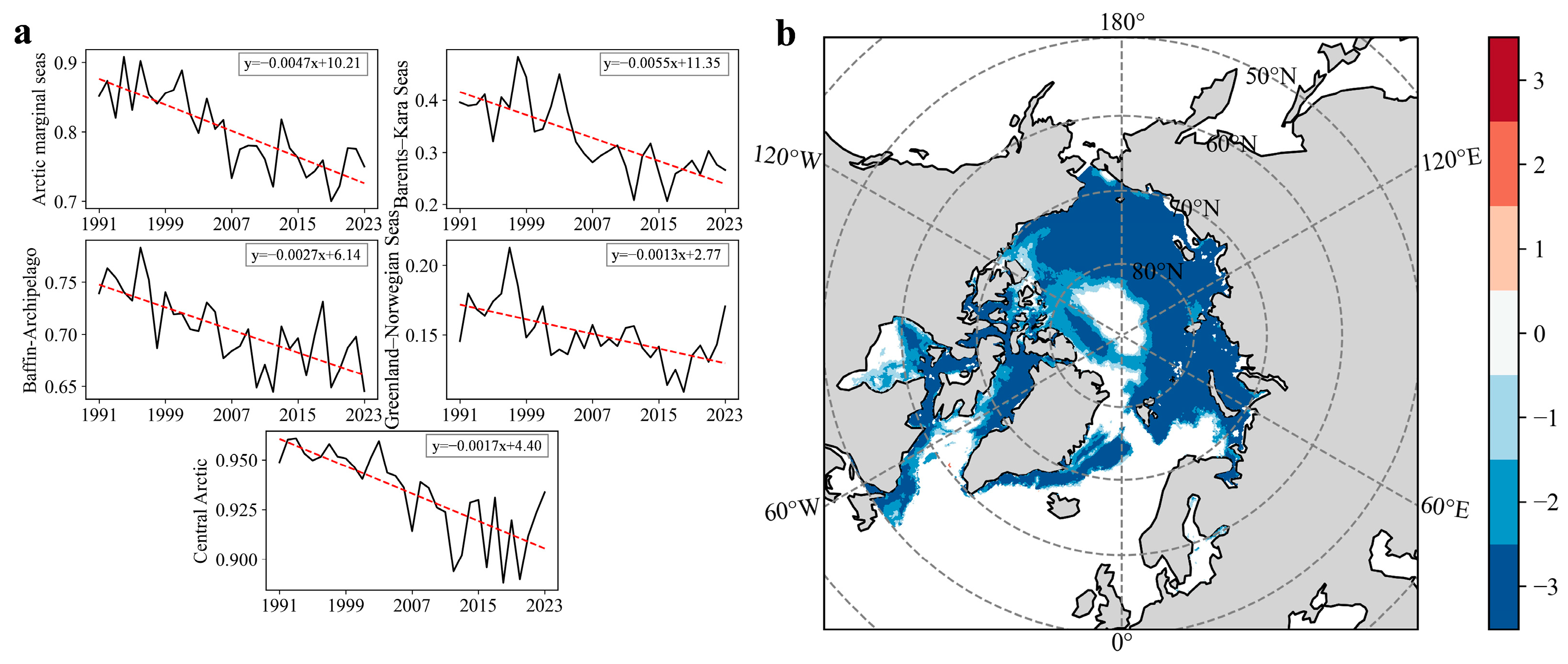
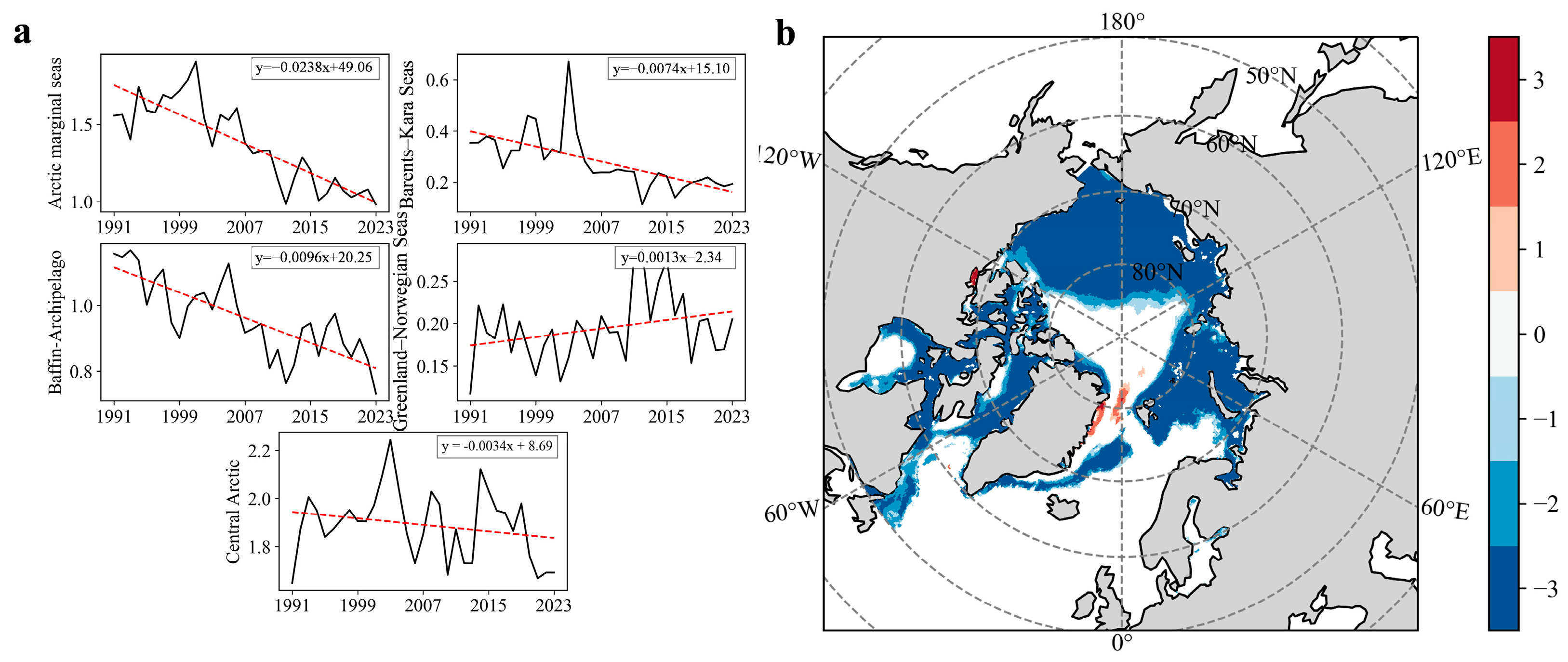
3.1. Spatiotemporal Variations in Arctic Sea Ice
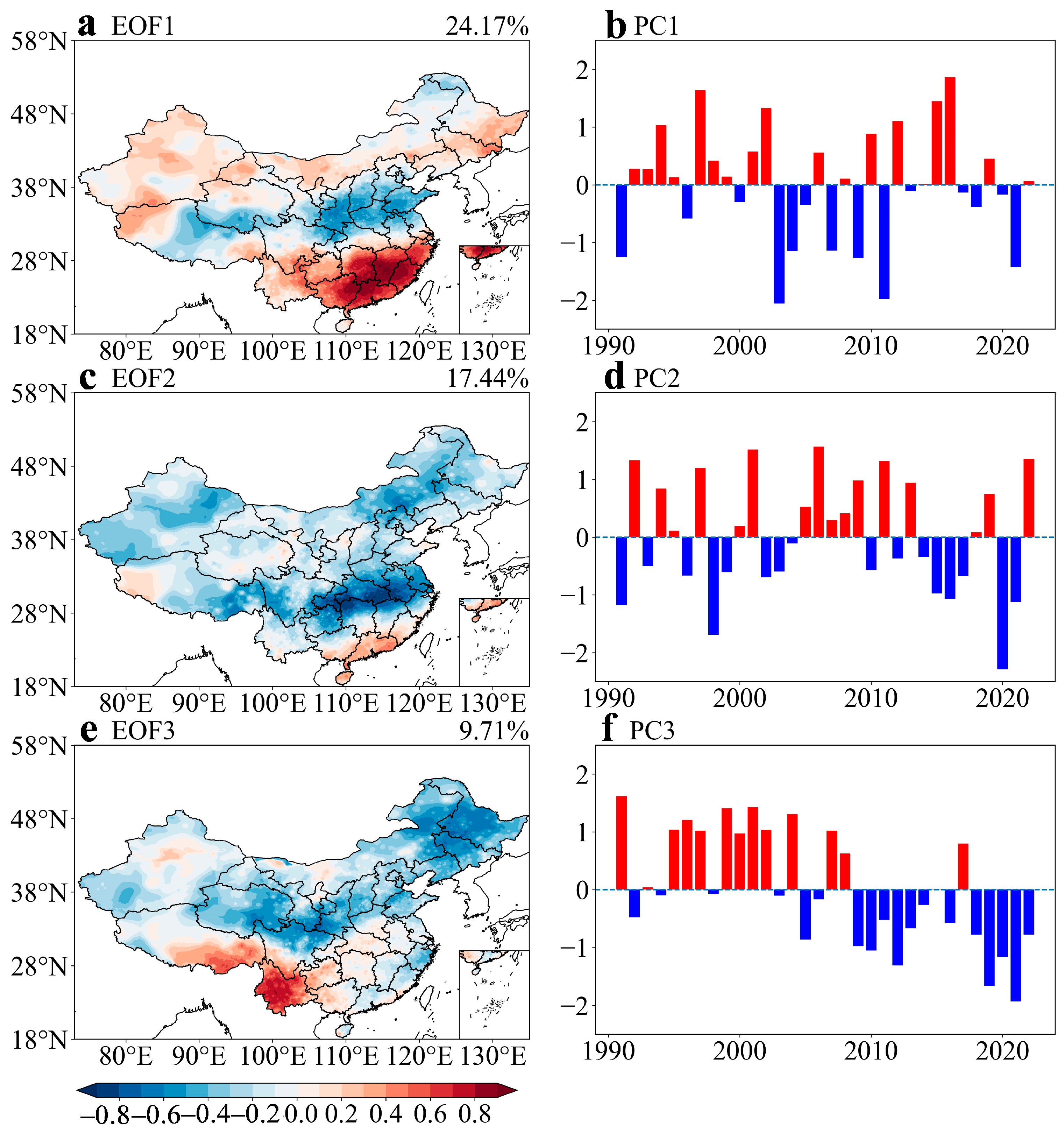
3.2. Spatiotemporal Variations in Precipitation in China
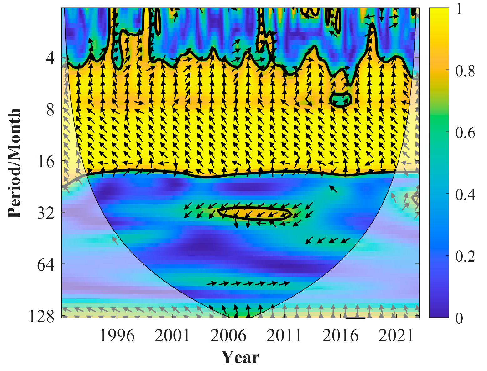
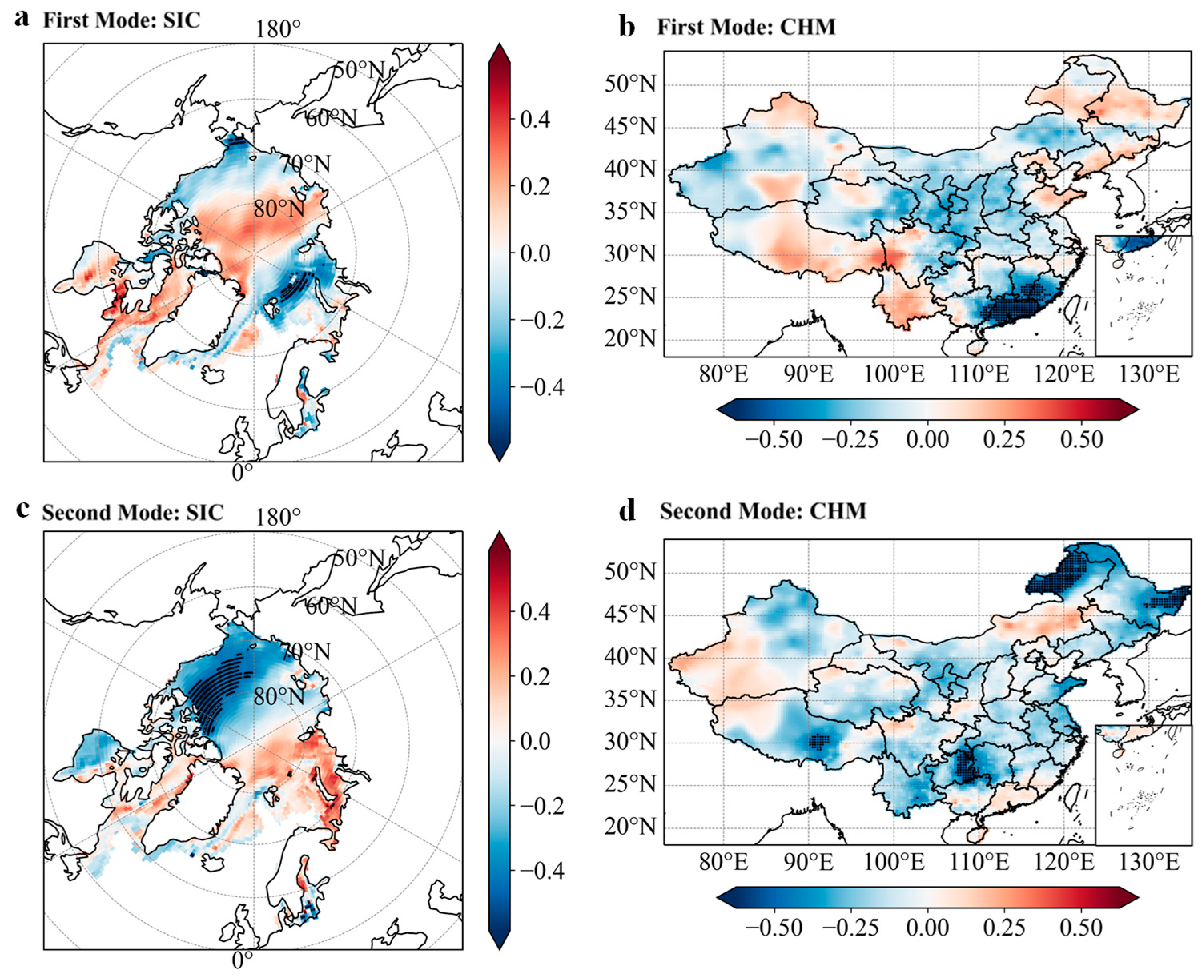
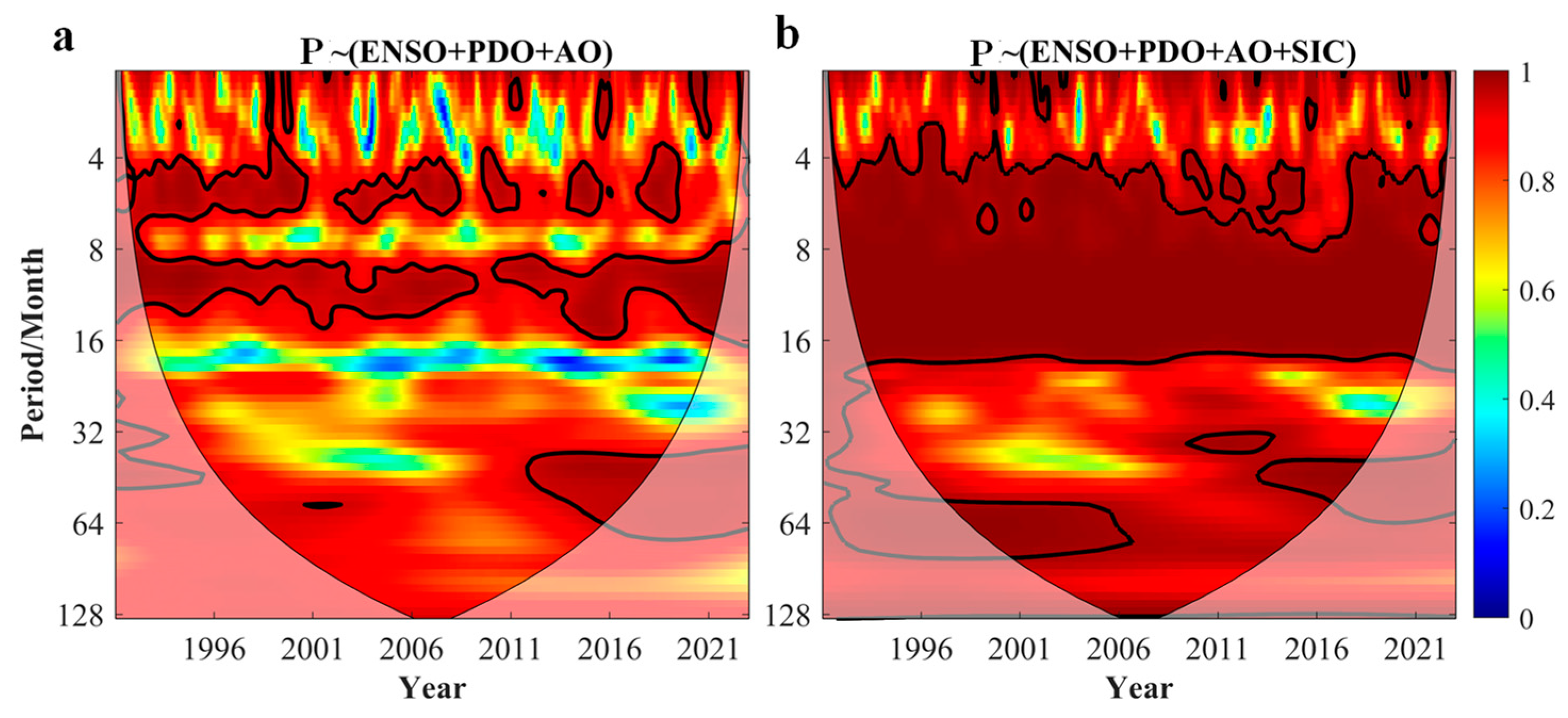
3.3. Time-Lag Effects of Arctic Sea Ice on Precipitation in China and Key Sea Area
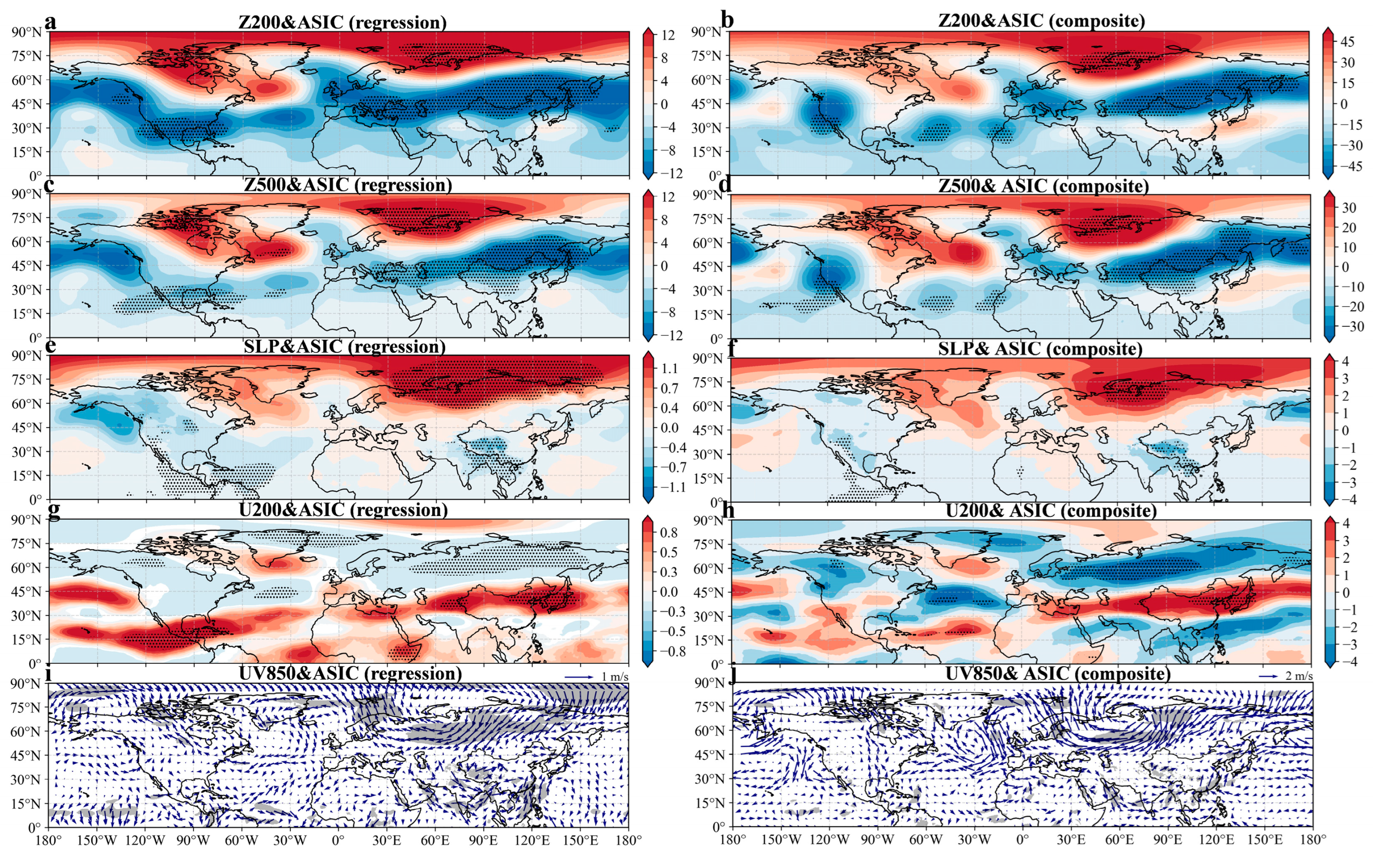
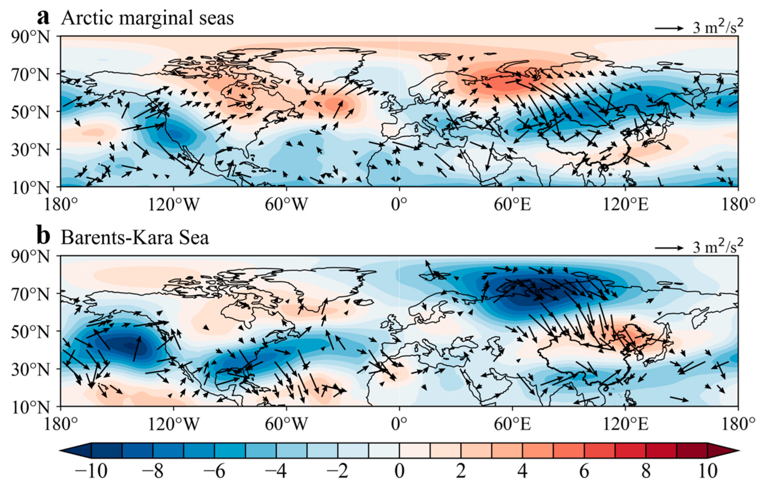
3.4. Response of Spring Atmospheric Circulation Anomalies to Winter Arctic Sea Ice Reduction
4. Discussion
5. Conclusions
Author Contributions
Funding
Data Availability Statement
Conflicts of Interest
References
- Screen, J.A.; Simmonds, I. The Central Role of Diminishing Sea Ice in Recent Arctic Temperature Amplification. Nature 2010, 464, 1334–1337. [Google Scholar] [CrossRef] [PubMed]
- Davy, R.; Griewank, P. Arctic Amplification Has Already Peaked. Environ. Res. Lett. 2023, 18, 084003. [Google Scholar] [CrossRef]
- Dai, A.; Luo, D.; Song, M.; Liu, J. Arctic Amplification Is Caused by Sea-Ice Loss under Increasing CO2. Nat. Commun. 2019, 10, 121. [Google Scholar] [CrossRef]
- Matveeva, T.A.; Semenov, V.A. Regional Features of the Arctic Sea Ice Area Changes in 2000–2019 versus 1979–1999 Periods. Atmosphere 2022, 13, 1434. [Google Scholar] [CrossRef]
- Wang, X.; Li, S.; Zhao, Y.; Wang, Y.; Yang, Z. Comparison of Arctic and Antarctic Sea Ice Spatial–Temporal Changes during 1979–2018. J. Hydrol. 2024, 632, 130966. [Google Scholar] [CrossRef]
- Guo, Y.; Wang, X.; Xu, H.; Hou, X. Spatiotemporal Variation and Freeze-Thaw Asymmetry of Arctic Sea Ice in Multiple Dimensions during 1979 to 2020. Acta Oceanol. Sin. 2024, 43, 102–114. [Google Scholar] [CrossRef]
- Jahn, A. Reduced Probability of Ice-Free Summers for 1.5 °C Compared to 2 °C Warming. Nat. Clim. Change 2018, 8, 409–413. [Google Scholar] [CrossRef]
- Wu, B.; Li, Z. Possible Impacts of Anomalous Arctic Sea Ice Melting on Summer Atmosphere. Intl J. Climatol. 2022, 42, 1818–1827. [Google Scholar] [CrossRef]
- Guo, D.; Gao, Y.; Bethke, I.; Gong, D.; Johannessen, O.M.; Wang, H. Mechanism on How the Spring Arctic Sea Ice Impacts the East Asian Summer Monsoon. Theor. Appl. Clim. 2014, 115, 107–119. [Google Scholar] [CrossRef]
- Zhang, S.; Zeng, G.; Yang, X.; Iyakaremye, V.; Hao, Z. Connection between Interannual Variation of Spring Precipitation in Northeast China and Preceding Winter Sea Ice over the Barents Sea. Intl J. Climatol. 2022, 42, 1922–1936. [Google Scholar] [CrossRef]
- Li, X.; Sun, J.; Zhang, M.; Zhang, Y.; Ma, J. Possible Connection between Declining Barents Sea Ice and Interdecadal Increasing Northeast China Precipitation in May. Intl J. Climatol. 2021, 41, 6270–6282. [Google Scholar] [CrossRef]
- Han, T.; Zhang, M.; Zhu, J.; Zhou, B.; Li, S. Impact of Early Spring Sea Ice in Barents Sea on Midsummer Rainfall Distribution at Northeast China. Clim. Dyn. 2021, 57, 1023–1037. [Google Scholar] [CrossRef]
- Zhao, P.; Zhang, X.; Zhou, X.; Ikeda, M.; Yin, Y. The Sea Ice Extent Anomaly in the North Pacific and Its Impact on the East Asian Summer Monsoon Rainfall. J. Clim. 2004, 17, 3434–3447. [Google Scholar] [CrossRef]
- Wu, B.; Zhang, R.; Wang, B. On the Association between Spring Arctic Sea Ice Concentration and Chinese Summer Rainfall: A Further Study. Adv. Atmos. Sci. 2009, 26, 666–678. [Google Scholar] [CrossRef]
- Wu, Z.; Li, X.; Li, Y.; Li, Y. Potential Influence of Arctic Sea Ice to the Interannual Variations of East Asian Spring Precipitation*. J. Clim. 2016, 29, 2797–2813. [Google Scholar] [CrossRef]
- Zuo, J.; Ren, H.-L.; Wu, B.; Li, W. Predictability of Winter Temperature in China from Previous Autumn Arctic Sea Ice. Clim. Dyn. 2016, 47, 2331–2343. [Google Scholar] [CrossRef]
- He, S.; Gao, Y.; Furevik, T.; Wang, H.; Li, F. Teleconnection between Sea Ice in the Barents Sea in June and the Silk Road, Pacific–Japan and East Asian Rainfall Patterns in August. Adv. Atmos. Sci. 2018, 35, 52–64. [Google Scholar] [CrossRef]
- Ricker, R.; Hendricks, S.; Kaleschke, L.; Tian-Kunze, X.; King, J.; Haas, C. A Weekly Arctic Sea-Ice Thickness Data Record from Merged CryoSat-2 and SMOS Satellite Data. Cryosphere 2017, 11, 1607–1623. [Google Scholar] [CrossRef]
- Han, J.; Miao, C.; Gou, J.; Zheng, H.; Zhang, Q.; Guo, X. A New Daily Gridded Precipitation Dataset for the Chinese Mainland Based on Gauge Observations. Earth Syst. Sci. Data 2023, 15, 3147–3161. [Google Scholar] [CrossRef]
- Hersbach, H.; Bell, B.; Berrisford, P.; Hirahara, S.; Horányi, A.; Muñoz-Sabater, J.; Nicolas, J.; Peubey, C.; Radu, R.; Schepers, D.; et al. The ERA5 Global Reanalysis. Quart. J. R. Meteoro Soc. 2020, 146, 1999–2049. [Google Scholar] [CrossRef]
- Da Costa, E.D. On the Invariance of the First EOF of North Atlantic Sea Level Pressure to Temporal Filtering. Geophys. Res. Lett. 2003, 30, 2003GL017312. [Google Scholar] [CrossRef]
- Bretherton, C.S.; Smith, C.; Wallace, J.M. An Intercomparison of Methods for Finding Coupled Patterns in Climate Data. J. Clim. 1992, 5, 541–560. [Google Scholar] [CrossRef]
- Takaya, K.; Nakamura, H. A Formulation of a Phase-Independent Wave-Activity Flux for Stationary and Migratory Quasigeostrophic Eddies on a Zonally Varying Basic Flow. J. Atmos. Sci. 2001, 58, 608–627. [Google Scholar] [CrossRef]
- Hu, W.; Si, B. Technical Note: Improved Partial Wavelet Coherency for Understanding Scale-Specific and Localized Bivariate Relationships in Geosciences. Hydrol. Earth Syst. Sci. 2021, 25, 321–331. [Google Scholar] [CrossRef]
- Su, L.; Miao, C.; Duan, Q.; Lei, X.; Li, H. Multiple-Wavelet Coherence of World’s Large Rivers With Meteorological Factors and Ocean Signals. JGR Atmos. 2019, 124, 4932–4954. [Google Scholar] [CrossRef]
- Grinsted, A.; Moore, J.C.; Jevrejeva, S. Application of the Cross Wavelet Transform and Wavelet Coherence to Geophysical Time Series. Nonlin. Process. Geophys. 2004, 11, 561–566. [Google Scholar] [CrossRef]
- Hu, W.; Si, B.C. Technical Note: Multiple Wavelet Coherence for Untangling Scale-Specific Andlocalized Multivariate Relationships in Geosciences. Hydrol. Earth Syst. Sci. 2016, 20, 3183–3191. [Google Scholar] [CrossRef]
- Hamed, K.H.; Ramachandra Rao, A. A Modified Mann-Kendall Trend Test for Autocorrelated Data. J. Hydrol. 1998, 204, 182–196. [Google Scholar] [CrossRef]
- Parkinson, C.L.; Cavalieri, D.J. Arctic Sea Ice Variability and Trends, 1979–2006. J. Geophys. Res. Ocean. 2008, 113. [Google Scholar] [CrossRef]
- Cavalieri, D.J.; Parkinson, C.L. Arctic Sea Ice Variability and Trends, 1979–2010. Cryosphere 2012, 6, 881–889. [Google Scholar] [CrossRef]
- Meier, W.; Stroeve, J. An Updated Assessment of the Changing Arctic Sea Ice Cover. Oceanog 2022. [Google Scholar] [CrossRef]
- Parkinson, C.L.; Comiso, J.C. On the 2012 Record Low Arctic Sea Ice Cover: Combined Impact of Preconditioning and an August Storm. Geophys. Res. Lett. 2013, 40, 1356–1361. [Google Scholar] [CrossRef]
- Mukherjee, A.; Ravichandran, M. Role of Atmospheric Heat Fluxes and Ocean Advection on Decadal (2000–2019) Change of Sea-Ice in the Arctic. Clim. Dyn. 2023, 60, 3503–3522. [Google Scholar] [CrossRef]
- Juszak, I.; Iturrate-Garcia, M.; Gastellu-Etchegorry, J.-P.; Schaepman, M.E.; Maximov, T.C.; Schaepman-Strub, G. Drivers of Shortwave Radiation Fluxes in Arctic Tundra across Scales. Remote Sens. Environ. 2017, 193, 86–102. [Google Scholar] [CrossRef]
- Tietsche, S.; Hawkins, E.; Day, J.J. Atmospheric and Oceanic Contributions to Irreducible Forecast Uncertainty of Arctic Surface Climate. J. Clim. 2016, 29, 331–346. [Google Scholar] [CrossRef]
- Jaiser, R.; Dethloff, K.; Handorf, D.; Cohen, J. Impact of Sea Ice Cover Changes on the Northern Hemisphere Atmospheric Winter Circulation. Tellus A Dyn. Meteorol. Oceanogr. 2012, 64, 11595. [Google Scholar] [CrossRef]
- Zou, C.; Zhang, R. Arctic Sea Ice Loss Modulates the Surface Impact of Autumn Stratospheric Polar Vortex Stretching Events. Geophys. Res. Lett. 2024, 51, e2023GL107221. [Google Scholar] [CrossRef]
- Petrie, R.E.; Shaffrey, L.C.; Sutton, R.T. Atmospheric Response in Summer Linked to Recent Arctic Sea Ice Loss. Quart. J. R. Meteoro Soc. 2015, 141, 2070–2076. [Google Scholar] [CrossRef]
- Outten, S.D.; Esau, I. A Link between Arctic Sea Ice and Recent Cooling Trends over Eurasia. Clim. Change 2012, 110, 1069–1075. [Google Scholar] [CrossRef]
- He, S.; Gao, Y.; Li, F.; Wang, H.; He, Y. Impact of Arctic Oscillation on the East Asian Climate: A Review. Earth-Sci. Rev. 2017, 164, 48–62. [Google Scholar] [CrossRef]
- Xiao, M.; Zhang, Q.; Singh, V.P. Influences of ENSO, NAO, IOD and PDO on Seasonal Precipitation Regimes in the Yangtze River Basin, China: Influences of ENSO Regimes on Precipitation. Int. J. Clim. 2015, 35, 3556–3567. [Google Scholar] [CrossRef]
- Chen, G.; Li, X.; Xu, Z.; Liu, Y.; Zhang, Z.; Shao, S.; Gao, J. PDO Influenced Interdecadal Summer Precipitation Change over East China in Mid-18th Century. npj Clim. Atmos. Sci. 2024, 7, 114. [Google Scholar] [CrossRef]
- Hussain, A.; Cao, J.; Ali, S.; Ullah, W.; Muhammad, S.; Hussain, I.; Abbas, H.; Hamal, K.; Sharma, S.; Akhtar, M.; et al. Wavelet Coherence of Monsoon and Large-scale Climate Variabilities with Precipitation in Pakistan. Intl J. Climatol. 2022, 42, 9950–9966. [Google Scholar] [CrossRef]
- Nalley, D.; Adamowski, J.; Biswas, A.; Gharabaghi, B.; Hu, W. A Multiscale and Multivariate Analysis of Precipitation and Streamflow Variability in Relation to ENSO, NAO and PDO. J. Hydrol. 2019, 574, 288–307. [Google Scholar] [CrossRef]


| Term | Definition |
|---|---|
| ENSO | El Niño-Southern Oscillation |
| PDO | Pacific Decadal Oscillation |
| AO | Arctic Oscillation |
| SIC | Sea Ice Concentration |
| SIT | Sea Ice Thickness |
| EOF | Empirical Orthogonal Function |
| SVD | Singular Value Decomposition |
| MWC | Multiple Wavelet Coherence |
| AWC | Average Wavelet Coherence |
| PASC | Percentage of Area with Significant Coherence |
| Z200 | 200 hPa Geopotential Height |
| Z500 | 500 hPa Geopotential Height |
| SLP | Sea Level Pressure |
| U200 | 200 hPa Zonal Wind |
| UV850 | 850 hPa Horizontal Wind |
Disclaimer/Publisher’s Note: The statements, opinions and data contained in all publications are solely those of the individual author(s) and contributor(s) and not of MDPI and/or the editor(s). MDPI and/or the editor(s) disclaim responsibility for any injury to people or property resulting from any ideas, methods, instructions or products referred to in the content. |
© 2025 by the authors. Licensee MDPI, Basel, Switzerland. This article is an open access article distributed under the terms and conditions of the Creative Commons Attribution (CC BY) license (https://creativecommons.org/licenses/by/4.0/).
Share and Cite
Wang, H.; Wang, W.; Guo, F. Time-Lag Effects of Winter Arctic Sea Ice on Subsequent Spring Precipitation Variability over China and Its Possible Mechanisms. Water 2025, 17, 1443. https://doi.org/10.3390/w17101443
Wang H, Wang W, Guo F. Time-Lag Effects of Winter Arctic Sea Ice on Subsequent Spring Precipitation Variability over China and Its Possible Mechanisms. Water. 2025; 17(10):1443. https://doi.org/10.3390/w17101443
Chicago/Turabian StyleWang, Hao, Wen Wang, and Fuxiong Guo. 2025. "Time-Lag Effects of Winter Arctic Sea Ice on Subsequent Spring Precipitation Variability over China and Its Possible Mechanisms" Water 17, no. 10: 1443. https://doi.org/10.3390/w17101443
APA StyleWang, H., Wang, W., & Guo, F. (2025). Time-Lag Effects of Winter Arctic Sea Ice on Subsequent Spring Precipitation Variability over China and Its Possible Mechanisms. Water, 17(10), 1443. https://doi.org/10.3390/w17101443