Progressive Linear Programming Optimality Method Based on Decomposing Nonlinear Functions for Short-Term Cascade Hydropower Scheduling

Abstract

Short-term optimal scheduling of cascade hydropower stations enhances their flexible regulation and power generation capabilities. However, nonlinear function relationships and multistage and hydraulic interdependencies present significant challenges, resulting in considerable solution errors, premature convergence, and high computational demands. This study proposes a progressive linear programming method that decomposes nonlinear functions to address these challenges. First, to accurately represent nonlinear functions and mitigate computational complexity, the entire feasible domain is partitioned into multiple contiguous subdomains in which nonconvex nonlinear functions within each subdomain can be equivalently replaced by linear relationships. Second, a progressive linear programming optimization algorithm is devised to prevent premature convergence, utilizing continuous subdomains rather than discrete points as state variables and incorporating the progressive optimality principle. Finally, to increase the solution efficiency, a dimensionality reduction strategy via the feasible domain state dynamic acquisition method is presented and optimized after excluding the infeasible states in each stage. The simulation of three cascade hydropower stations in a river basin in southwest China shows that the proposed method can achieve a superior peak regulation effect compared to the conventional mixed integer linear programming and progressive optimality algorithm. During the dry and wet seasons, the residual load peak–valley differences at the three stations are reduced by 612 MW and 521 MW compared to the MILP and 1889 MW and 2439 MW compared to the POA, which underscores the effectiveness of the method in optimizing the short-term scheduling of cascade hydropower stations.

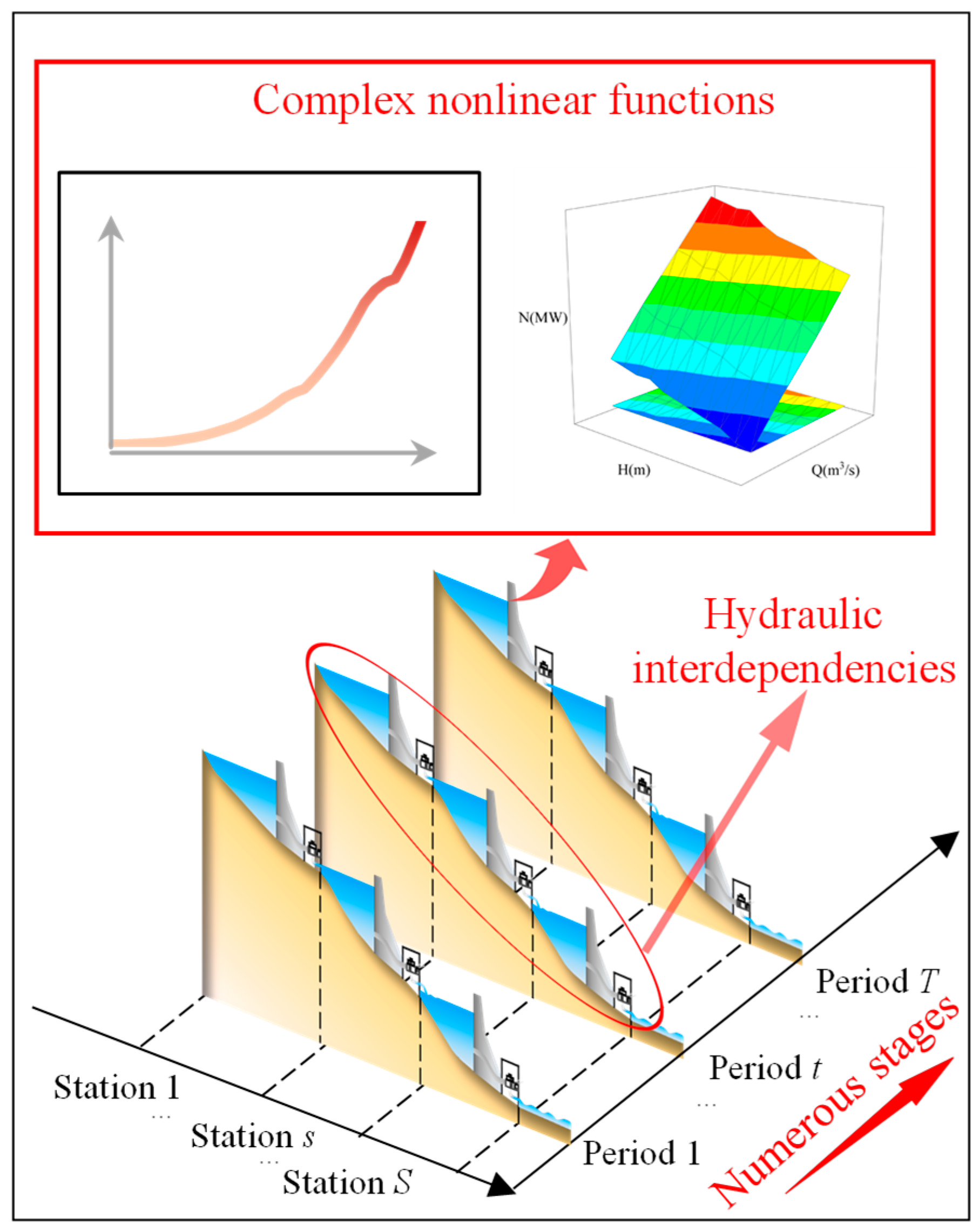
1. Introduction

Extreme weather conditions, such as high temperatures and severe cold, coupled with the uncertainty of renewable energy sources, are intensifying the challenges faced by power systems in power supplies [1,2]. According to data from 2023, the load of 30 provincial-level power grids in China reached a new peak, with the maximum load increasing by 50 million kilowatts compared with that in 2022. Cascade hydropower stations, with significant power generation and regulation capabilities, play a crucial role in ensuring the supply reliability and balance of the power grid as a clean energy source [3,4]. However, the short-term optimal scheduling of cascade hydropower stations (STOSCHS) is complicated by factors such as complex nonlinear functions (NLFs), numerous stages, and large variable scales, posing significant challenges when exploring solutions [5,6]. As illustrated in Figure 1, the operational characteristics of hydropower stations give rise to complex nonlinear constraints. The close hydraulic connections between cascades complicate the separation of upstream and downstream segments. The scale of the problem increases exponentially with the number of hydropower stations, and the current demands for refined scheduling necessitate more detailed dispatching timeframes. These factors contribute to challenges related to imprecision, suboptimal solutions, and slow computation. Current existing methods and algorithms struggle to meet the requirements of solution accuracy, optimization depth, and timeliness simultaneously [7,8,9]. Therefore, further research into methods suitable for the STOSCHS is still required.

One significant difficulty in the STOSCHS problem lies in the complex NLFs. These NLFs are derived from a series of discrete points through actual experimental testing and cannot be accurately described by elementary functions, making both precise modeling and solutions highly challenging. To mitigate the significant computational challenges posed by NLFs, extensive research has focused on approximating them to facilitate efficient solution methods, which can be broadly categorized into three main types. First, the NLFs are relaxed by fixing the water head, followed by iterative updates to the water head after finding a solution [10,11,12]. However, this method is prone to oscillations during the iteration process and has difficulty converging. Second, NLFs are fitted with continuous polynomials to construct and solve a nonlinear programming model [13,14,15]. Nevertheless, both the accuracy of the fit and the solution to the nonlinear programming model were challenging. Third, integer variables are introduced to formulate a mixed integer linear programming (MILP) model, and the number of discrete points is reduced or approximate interpolation is employed to simplify the model for easier solutions [16,17,18]. Fang et al. approximated the NLFs using two linear segments and eight triangles, thereby developing a MILP model for short-term peak shaving that alleviated the difficulties posed by the nonlinearity of NLFs [17]. Nonetheless, a significant number of approximations may result in cumulative errors. In summary, the results obtained from these methods need further verification and adjustment to eliminate errors. For short-term operations that require high accuracy, direct application of their results cannot provide practical guidance for production. Therefore, it is imperative to investigate how to achieve high-quality STOSCHS solutions with precise handling of NLFs.

To obtain directly applicable short-term scheduling solutions, extensive research has focused on algorithms that are capable of solving precise short-term scheduling models. The mainstream approaches predominantly include evolutionary algorithms and dynamic programming algorithms. Evolutionary algorithms, such as the genetic algorithm [19], particle swarm optimization [20], ant colony optimization [21], invasive weed optimal algorithm [22], and simulated annealing [23], typically leverage random numbers to construct solution frameworks, thus achieving higher solution efficiency without the need to traverse all states. Nevertheless, the use of random numbers can lead to instability in intelligent algorithm solutions, posing significant challenges for retrospective analysis of scheduling schemes and increasing the likelihood of premature convergence. Dynamic programming algorithms [24], which are suitable for multistage decision problems, have been extensively utilized in research on optimizing scheduling for hydropower stations. However, characteristics such as load regulation and delayed water flow in short-term scheduling require the simultaneous consideration of relationships between multiple stages, which contradicts the property of dynamic programming algorithms that assume no aftereffect, thus posing challenges for conventional dynamic programming [25], discrete differential dynamic programming [26], and dynamic programming with successive approximations [27]. The progressive optimality algorithm (POA) can partially overcome the limitation of no aftereffect. Feng et al. developed a parallel POA for peak load scheduling in cascade hydropower stations, successfully reducing the residual load peak-to-valley difference from 4821.3 MW to 1728.6 MW across 10 hydropower stations with a total installed capacity of 9025 MW [28]. However, fixing the states for non-computational periods may lead the POA to become trapped in premature convergence. Therefore, achieving deep STOSCHS optimization remains highly relevant and practical.

Precise and deep optimization often results in larger variable scales and computational complexity, which conflicts with the timeliness required for short-term scheduling. Consequently, extensive research has focused on dimensionality reduction methods to address this issue. On a temporal scale, loads can be categorized into base loads and peak loads to reduce the number of stages during the solution process, thereby achieving faster solutions [29]. On a spatial scale, the entire cascade can be decomposed into multiple segments and iteratively solved to decrease the complexity of each solution iteration [30]. These studies employ a divide-and-conquer approach, breaking down complex problems into a series of simpler problems to effectively reduce the dimension. However, these methods are prone to premature convergence and sacrifice some of their solution quality in the process. Parallel techniques enable faster attainment of cascade hydropower scheduling results without compromising optimization quality. This approach enhances the solution speed by distributing tasks that do not require sequential execution across multiple processors simultaneously [31]. Nonetheless, integrating parallel techniques with algorithmic logic is challenging and demands increased hardware resources. Analyzing the feasibility domain of the problem prior to finding a solution and reducing the number of computations in infeasible domains to lower the solution complexity are other effective dimensionality reduction strategies that do not compromise the solution quality [32]. Existing studies often refine the state space before finding a solution to avoid unnecessary computations [33]. However, the close interconnection between time periods results in mutual influence among the feasibility of states across different periods. The number of absolutely infeasible states is limited, thus limiting the extent of dimensionality reduction. Therefore, determining feasible states on the basis of the interrelationships between states across time periods during the optimization process is an effective approach for achieving substantial dimensionality reduction.

To address the conflicts among precision, depth of optimization, and scale when solving STOSCHS problems, this study innovatively proposes a progressive linear programming optimality method based on decomposing nonlinear functions (PLPOMDNF) that aims to increase the power supply capability of cascade hydropower stations. This paper makes the following contributions:

(1) Partitioning feasible domains coupled with NLF characteristics. NLFs, including the forebay water level–water storage function, tailrace water level–power water release function, and power output–water head–power water release function, are discretely decomposed into adjacent linear segments or triangles according to discrete points obtained through practical experiments. Based on the decomposition of these NLFs, the feasible domain is subdivided into a series of subdomains, where every nonlinear relationship in each subdomain is equivalent to a linear relationship. This partitioning method effectively eliminates the complex NLFs of each hydropower station without introducing approximation errors.

(2) Progressive linear programming optimality algorithm with continuous domain states. The progressive optimality principle, which is suitable for solving multistage problems, is adopted to ensure monotonic convergence. The resulting decomposed subdomains are treated as states for each power station, referred to as domain states, and each decision made while updating the state is efficiently solved via linear programming. By treating continuous subdomains as states rather than fixed discrete points, the algorithm ensures that states from all stages can be adjusted during each optimization step, enhancing the convergence of the objective function and the ability to escape local optima.

(3) Dimension reduction strategy via the feasible domain state dynamic acquisition method. Based on the optimization logic of the progressive linear programming optimality algorithm, a feasible domain state dynamic acquisition method is proposed. This method utilizes domain states from other non-optimization stages and the feasible range of current stage variables as input conditions, aiming to reduce the number of states prior to optimization at the current stage. To accurately determine the feasible range of current stage variables, an approach involving variable boundary calculation linear programming (VBCLP) is designed. This dimension reduction strategy effectively filters out infeasible domain states, avoiding useless calculations.

The remaining structure of this paper is as follows: Section 2 introduces the mathematical model for the short-term optimal scheduling of cascade hydropower stations. Section 3 describes the detailed theoretical methods and operational processes of PLPOMDNF employed to solve the STOSCHS, and Section 4 presents a case study validating the proposed method. Finally, Section 5 provides conclusions and outlines future research plans.

2. Model Formulation

2.1. Objective Function

The primary purpose of the short-term optimal scheduling of cascade hydropower stations involves optimizing the daily power output process under given initial and ending forebay water levels. This process aims to minimize the peak–valley difference of the residual load to stabilize the power demand of other types of power sources with insufficient regulation capacity, so the objective function Equation (1) is adopted. All the symbols can be found with their specific meanings in Section Abbreviations.

$$\min F^{\mathrm{STOS}}=\underset{t\in T}{\max }\left\{l_t^{\mathrm{R}}\right\}-\underset{t\in T}{\min }\left\{l_t^{\mathrm{R}}\right\}$$

(1)

$$l_t^{\mathrm{R}}=L{D}_t-{\displaystyle \sum _{s\in S}{p}_{s,t}}(\forall t\in T)$$

(2)

Since Equation (1) is nonlinear, two auxiliary variables $l{a}^{\max }$ and $l{a}^{\min }$ are introduced to linearize it into Equation (3).

$$\min F^{\mathrm{STOS}}=l{a}^{\max }-l{a}^{\min }$$

(3)

$$l{a}^{\max }\ge l_t^{\mathrm{R}}\hspace{1em}(\forall t\in T)$$

(4)

$$l{a}^{\min }\le l_t^{\mathrm{R}}\hspace{1em}(\forall t\in T)$$

(5)

2.2. Constraints

The constraints of the model can be classified into linear Constraints (6)~(15) and nonlinear Constraints (16)~(19) [17,30].

2.2.1. Linear Constraints

• The continuity water balance constraint:

$$v_{s,t}=v_{s,t-1}+\left(i_{s,t}-q_{s,t}\right)\times \Delta t\hspace{1em}(\forall s\in S,\forall t\in T)$$

(6)

Constraint (6) represents the relationship between the variation in water storage and total inflow and power water release, indicating that the total water volume within a time period is conserved.

2.

The complex hydraulic connection:

$$i_{s,t}=\left\{\begin{array}{cc}I{N}_{s,t}& (\forall s\in S_1,\forall t\in T)\\ \begin{array}{l}\\ I{N}_{s,t}+{\displaystyle \sum _{\begin{array}{c}{s}^{\prime }\in S_s^{\mathrm{up}}\\ t-T_{s^{\prime }}^{\mathrm{lag}}\in T\end{array}}{q}_{s^{\prime },t-T_{s^{\prime }}^{\mathrm{lag}}}}\end{array}& (\forall s\in S_2,\forall t\in T)\end{array}\right.$$

(7)

Constraint (7) represents the relationship between the power water release from the upstream station and the total inflow to the downstream station, indicating that the total water volume between the upstream and downstream stations is conserved.

3.

The ecological flow constraint:

$$q_{s,t}\ge Q_s^{\mathrm{eco}} (\forall s\in S,\forall t\in T)$$

(8)

Constraint (8) indicates that the ecological protection requirements impose a lower bound on the discharge flow released by the hydropower station during each time period.

4.

The shipping water level constraint:

$$z{d}_{s,t}\ge Z_s^{\mathrm{ship}} (\forall s\in S,\forall t\in T)$$

(9)

Constraint (9) indicates that the shipping requirements impose a lower bound on the tailrace water level of the hydropower station during each time period.

5.

The forebay water level constraints:

$$\underset{¯}{Z{F}_s}\le z{f}_{s,t}\le \overline{Z{F}_s} (\forall s\in S,\forall t\in T)$$

(10)

Constraint (10) stipulates that the forebay water level must remain within a specified range. Typically, the minimum value corresponds to the dead water level of the reservoir, while the maximum value is the normal water level during the dry season and the flood control water level during the flood season.

6.

The power water release constraints:

$$\underset{¯}{Q_s}\le q_{s,t}\le \overline{Q_s} (\forall s\in S,\forall t\in T)$$

(11)

Constraint (11) stipulates that the power water release of the hydropower station must remain within a specific range, which is typically determined by the parameters of the generating equipment.

7.

The power output constraints:

$$\underset{¯}{P_s}\le p_{s,t}\le \overline{P_s} (\forall s\in S,\forall t\in T)$$

(12)

Constraint (12) indicates that the power output of the hydropower station must lie within a specified range, which is generally associated with the parameters of the generating equipment.

8.

The power output ramp-up and ramp-down constraints:

$$-\Delta p_s\le p_{s,t+1}-p_{s,t}\le \Delta p_s (\forall s\in S,t\in T,t\ne T)$$

(13)

Constraint (13) defines that the variation in the power output of the hydropower station between consecutive time periods is constrained, with these limitations generally being associated with the parameters of the generating equipment.

9.

The initial and final forebay water level constraints:

$$z{f}_{s,0}=Z_s^{\mathrm{beg}} (\forall s\in S)$$

(14)

$$z{f}_{s,\mathrm{T}}=Z_s^{\mathrm{end}} (\forall s\in S)$$

(15)

Constraints (14) and (15) define the forebay water levels at the beginning and end of the scheduling period for the hydropower station, respectively.

2.2.2. Nonlinear Constraints

• The relationship between head loss and power water release:

$$h_{s,t}^{\mathrm{loss}}=f_s^{\mathrm{loss}}\left(q_{s,t}\right) (\forall s\in S,\forall t\in T)$$

(16)

Constraint (16) indicates that the head loss is a function of the power water release. Typically, the head loss is proportional to the square of the power water release.

2.

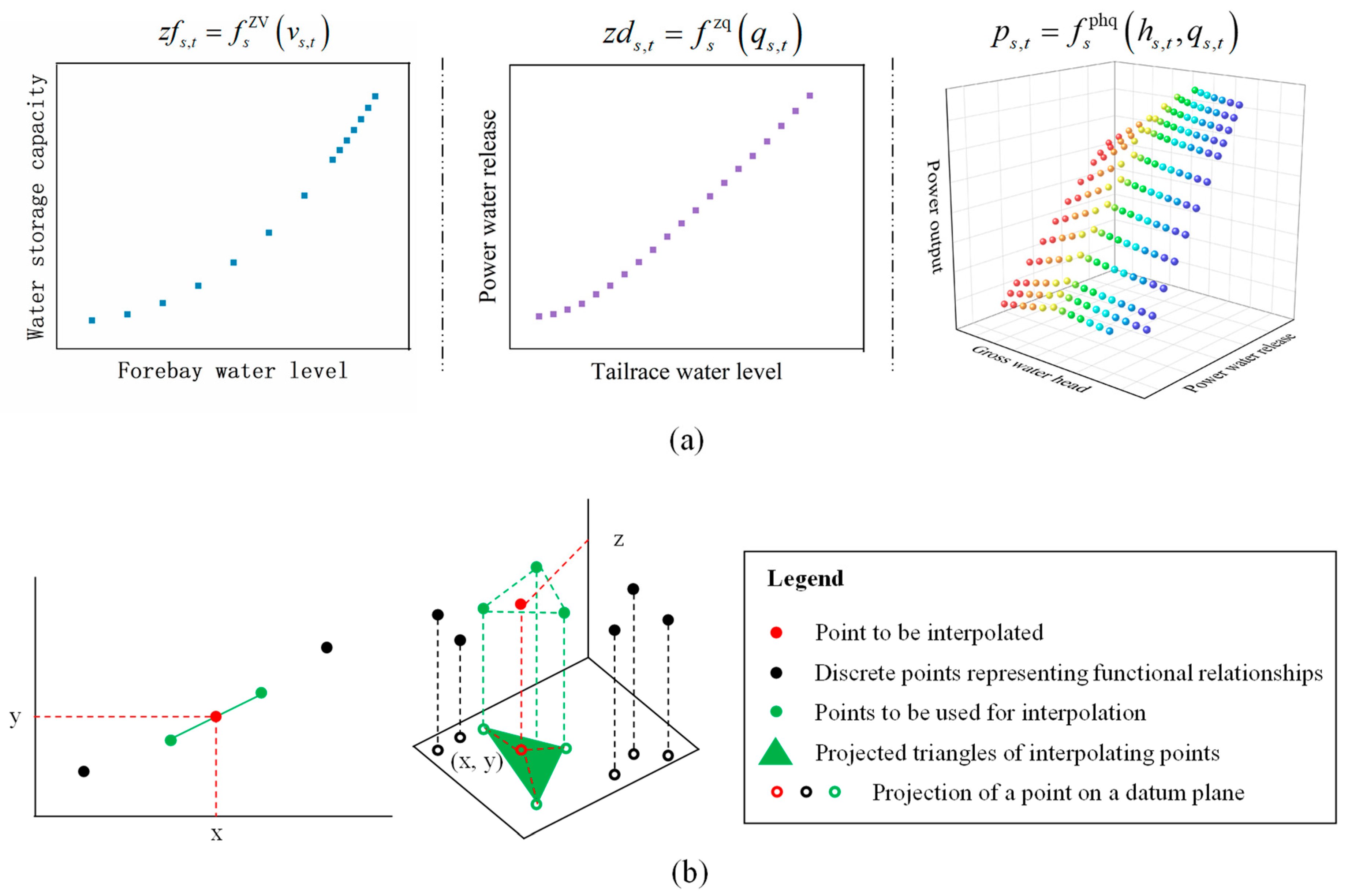
The functional relationship between the forebay water level and water storage:

$$z{f}_{s,t}=f_s^{\mathrm{zv}}\left(v_{s,t}\right) (\forall s\in S,\forall t\in T)$$

(17)

Constraint (17) represents the functional relationship between the water storage and the forebay water level, which is a monotonically increasing function.

3.

The functional relationship of the tailrace water level and power water release:

$$z{d}_{s,t}=f_s^{\mathrm{zq}}\left(q_{s,t}\right) (\forall s\in S,\forall t\in T)$$

(18)

Constraint (18) represents the functional relationship between the power water release and the tailrace water level, which is a monotonically increasing function.

4.

The hydropower output formula:

$$p_{s,t}=f_s^{{\mathrm{ph}}^{\mathrm{n}}\mathrm{q}}\left(h_{s,t}^{\mathrm{net}},q_{s,t}\right) (\forall s\in S,\forall t\in T)$$

(19)

where $h_{s,t}^{\mathrm{net}}$ can be calculated by the following formula:

$$h_{s,t}^{\mathrm{net}}={\displaystyle \frac{z{f}_{s,t-1}+z{f}_{s,t}}{2}}-z{d}_{s,t}-h_{s,t}^{\mathrm{loss}} (\forall s\in S,\forall t\in T)$$

(20)

Constraint (19) represents the functional relationship among the power output, net water head, and power water release, which is a bivariate nonlinear function. Constraint (20) represents the net water head calculation formula. The net water head is related to the forebay water level, tailrace water level, and head loss.

2.3. Reduction of Model Nonlinearities

The analysis of the above model shows that the calculation of the net water head in Equation (20) serves the calculation of the power output in Equation (19). To reduce the nonlinearity in the model, the gross water head is introduced as follows:

$$h_{s,t}={\displaystyle \frac{z{f}_{s,t-1}+z{f}_{s,t}}{2}}-z{d}_{s,t} (\forall s\in S,\forall t\in T)$$

(21)

Equation (21) is transformed into Equation (22), denoted as the PHQ function, while Equation (16) is removed.

$$p_{s,t}=f_s^{{\mathrm{ph}}^{\mathrm{n}}\mathrm{q}}\left[h_{s,t}-f_s^{\mathrm{hq}}\left(q_{s,t}\right),q_{s,t}\right]=f_s^{\mathrm{phq}}\left(h_{s,t},q_{s,t}\right) (\forall s\in S,\forall t\in T)$$

(22)

In summary, the objective function (3) and the Constraints (2), (4)~(15), (17)~(18) and (21)~(22) collectively constitute the STOSCHS model.

3. Methods

The solution to the STOSCHS model is a high-dimensional nonlinear problem that is constrained by premature convergence, convergence oscillation, multiple stages, and a large variable scale. The proposed PLPOMDNF can transform the original complex problem into an iterative linear programming problem with monotonic convergence based on an initial feasible solution. Initially, the STOSCHS NLFs are decomposed into a series of continuous subdomains according to their characteristics. Within each subdomain, the original NLFs are substituted with a set of linear constraints. Then, the progressive optimality principle is adopted to update the combinatorial domain state trajectory, and each state transition decision is a linear programming solution problem. Finally, a feasible domain state dynamic acquisition method based on optimization logic is designed to reduce the number of states and mitigate the curse of dimensionality.

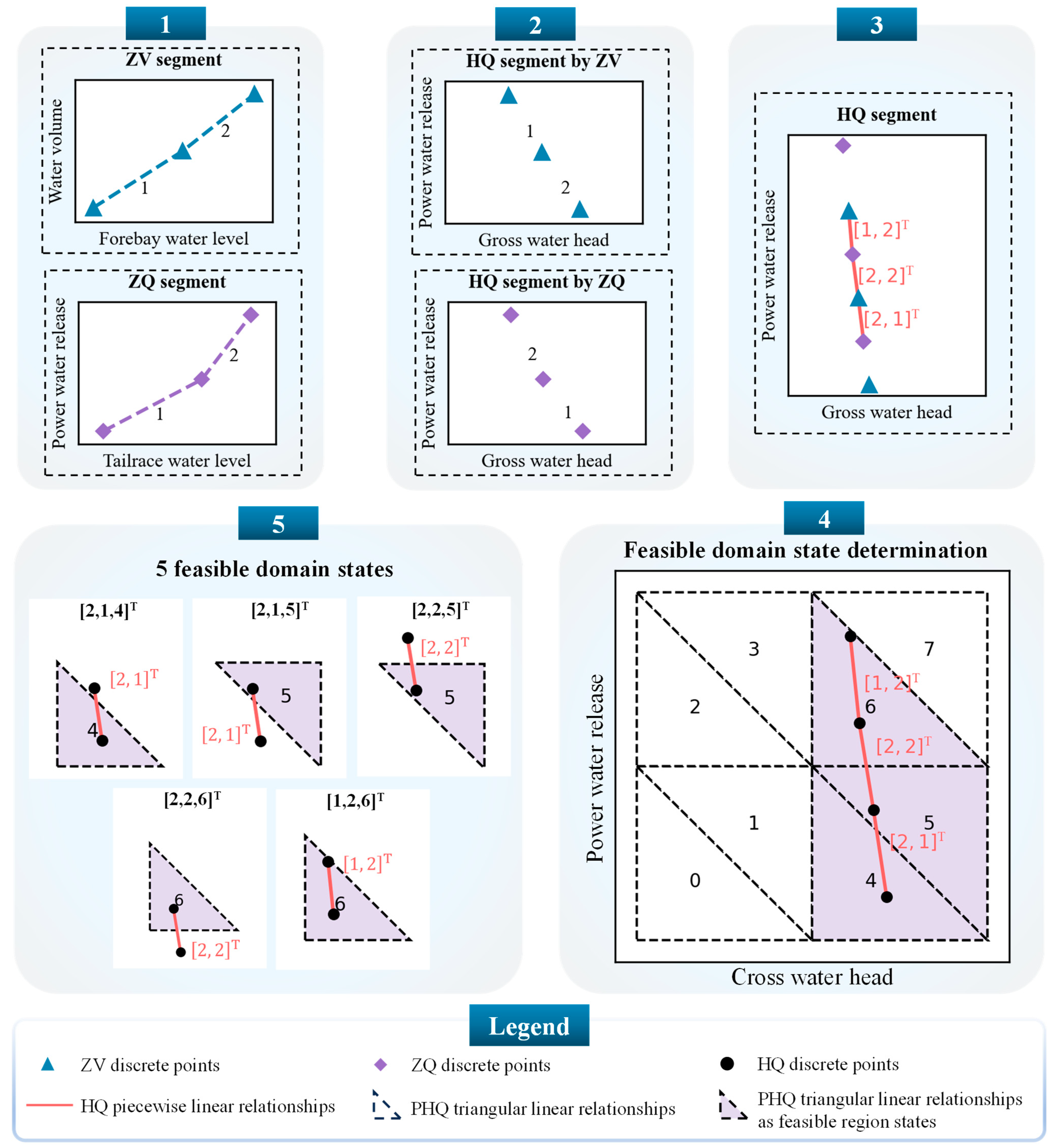
3.1. Partitioning Feasible Domains Coupled with NLF Characteristics

3.1.1. NLFs of Hydropower Stations

The nonlinear functional relationships for each hydropower station consist of a series of discrete points obtained through practical experiments, which defy precise description by elementary functions. Figure 2a illustrates the discrete points representing the real nonlinear functional relationships of a hydropower station, with particular emphasis on the complexity of the PHQ function. Typically, as the water head increases, the water consumption rate (the amount of water consumed per unit of electricity generated) decreases. However, at the same water head, the water consumption rate exhibits irregular variations as the power water release increases. Hence, precise characterization of these functional relationships is essential. For two-dimensional functional relationships, such as the ZV function and ZQ function, and three-dimensional functional relationships, such as the PHQ function, using piecewise linear interpolation and trigonometric linear interpolation, respectively, can effectively preserve the relationship between experimental data points. Figure 2b demonstrates the method used to obtain function values from these discrete points. Consequently, a nonlinear functional relationship can be delineated by a collection of line segments defined by two adjacent points for a two-dimensional function or by a set of triangular planes defined by three adjacent points for a three-dimensional function. In this study, the nonlinear functional relationships embodied in Equations (17), (18), and (22) are denoted as the ZV segment, ZQ segment, and PHQ grid, respectively.

3.1.2. Partitioning the Feasible Domains of One Hydropower Station

To calculate the value of a nonlinear function, we must determine which segment or triangle the point lies within. By indexing each line segment of the ZV segment and ZQ segment and each triangle of the PHQ grid, the state of hydropower station $s$ at period $t$ can correspond to an index vector $\overrightarrow{j_{s,t}}={\left[j_{s,t}^{\mathrm{zv}},j_{s,t}^{\mathrm{zq}},j_{s,t}^{\mathrm{phq}}\right]}^{\mathrm{T}}$. This vector denotes that $z{f}_{s,t}$ and $v_{s,t}$ lie within linear segment $j_{s,t}^{\mathrm{zv}}$; $z{d}_{s,t}$ and $q_{s,t}$ reside in linear segment $j_{s,t}^{\mathrm{zq}}$; and $h_{s,t}$, $q_{s,t}$, and $p_{s,t}$ are situated within linear triangle $j_{s,t}^{\mathrm{phq}}$. In other words, the index vector $\overrightarrow{j_{s,t}}={\left[j_{s,t}^{\mathrm{zv}},j_{s,t}^{\mathrm{zq}},j_{s,t}^{\mathrm{phq}}\right]}^{\mathrm{T}}$ represents a subdomain in which all of the variables satisfy the linear constraints of Equations (23)~(25).

$$\left\{\begin{array}{l}z{f}_{s,t}-\underset{¯}{Z{F}_{s,j_{s,t}^{\mathrm{zv}}}^{\mathrm{line}}}={\displaystyle \frac{\overline{Z{F}_{s,j_{s,t}^{\mathrm{zv}}}^{\mathrm{line}}}-\underset{¯}{Z{F}_{s,j_{s,t}^{\mathrm{zv}}}^{\mathrm{line}}}}{\overline{V_{s,j_{s,t}^{\mathrm{zv}}}^{\mathrm{line}}}-\underset{¯}{V_{s,j_{s,t}^{\mathrm{zv}}}^{\mathrm{line}}}}}\times \left(v_{s,t}-\underset{¯}{V_{s,j_{s,t}^{\mathrm{zv}}}^{\mathrm{line}}}\right)\\ \underset{¯}{V_{s,j_{s,t}^{\mathrm{zv}}}^{\mathrm{line}}}\le v_{s,t}\le \overline{V_{s,j_{s,t}^{\mathrm{zv}}}^{\mathrm{line}}}\end{array}\right. (\forall s\in S,\forall t\in T)$$

(23)

$$\left\{\begin{array}{l}z{d}_{s,t}-\underset{¯}{Z{D}_{s,j_{s,t}^{\mathrm{zv}}}^{\mathrm{line}}}={\displaystyle \frac{\overline{Z{D}_{s,j_{s,t}^{\mathrm{zv}}}^{\mathrm{line}}}-\underset{¯}{Z{D}_{s,j_{s,t}^{\mathrm{zv}}}^{\mathrm{line}}}}{\overline{Q_{s,j_{s,t}^{\mathrm{zv}}}^{\mathrm{line}}}-\underset{¯}{Q_{s,j_{s,t}^{\mathrm{zv}}}^{\mathrm{line}}}}}\times \left(q_{s,t}-\underset{¯}{Q_{s,j_{s,t}^{\mathrm{zv}}}^{\mathrm{line}}}\right)\\ \underset{¯}{Q_{s,j_{s,t}^{\mathrm{zq}}}^{\mathrm{line}}}\le q_{s,t}\le \overline{Q_{s,j_{s,t}^{\mathrm{zq}}}^{\mathrm{line}}}\end{array}\right. (\forall s\in S,\forall t\in T)$$

(24)

$$\left\{\begin{array}{l}{h}_{s,t}={\alpha }_{s,t}\times H{A}_{s,j_s^{\mathrm{phq}}}^{tri}+{\beta }_{s,t}\times H{B}_{s,j_s^{\mathrm{phq}}}^{tri}+{\gamma }_{s,t}\times H{C}_{s,j_s^{\mathrm{phq}}}^{tri}\\ q_{s,t}={\alpha }_{s,t}\times Q{A}_{s,j_{s,t}^{\mathrm{phq}}}^{tri}+{\beta }_{s,t}\times Q{B}_{s,j_{s,t}^{\mathrm{phq}}}^{tri}+{\gamma }_{s,t}\times Q{C}_{s,j_{s,t}^{\mathrm{phq}}}^{tri}\\ p_{s,t}={\alpha }_{s,t}\times P{A}_{s,j_{s,t}^{\mathrm{phq}}}^{tri}+{\beta }_{s,t}\times P{B}_{s,j_{s,t}^{\mathrm{phq}}}^{tri}+{\gamma }_{s,t}\times P{C}_{s,j_{s,t}^{\mathrm{phq}}}^{tri}\\ {\alpha }_{s,t}+{\beta }_{s,t}+{\gamma }_{s,t}=1\\ {\alpha }_{s,t}\ge 0, {\beta }_{s,t}\ge 0, {\gamma }_{s,t}\ge 0\end{array}\right. (\forall s\in S,\forall t\in T)$$

(25)

A subdomain corresponds to a continuous space, and all subdomains are mutually exclusive and together form the continuous space defined by nonlinear constraints. The total number of subdomains can be obtained via Equation (26).

$$K_s^{\mathrm{total}}=K_s^{\mathrm{zv}}\times K_s^{\mathrm{zq}}\times K_s^{\mathrm{phq}} (\forall s\in S)$$

(26)

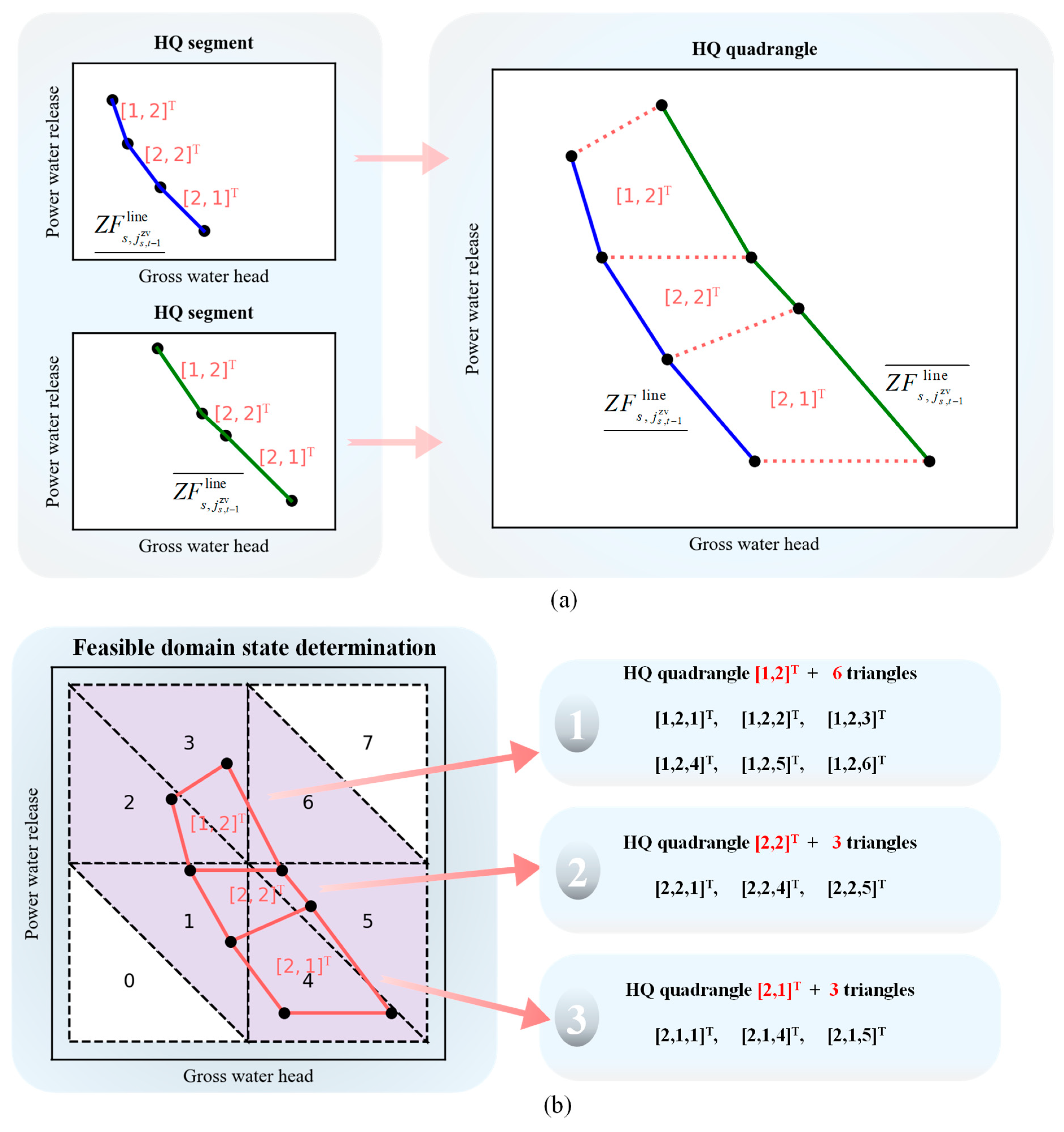
3.1.3. Combinatorial Subdomains of Cascade Hydropower Stations

The combinatorial subdomain of stage $t$, denoted as the matrix in Equation (27), is obtained through the Cartesian combination of subdomains from each station. This matrix comprises the ZV segment indices, ZQ segment indices, and PHQ grid indices of all of the stations.

$$J_t=\left[\overrightarrow{j_{1,t}},\overrightarrow{j_{2,t}},\dots ,\overrightarrow{j_{S,t}}\right]=\left[\begin{array}{llll}{j}_{1,t}^{\mathrm{zv}}\hfill & j_{2,t}^{\mathrm{zv}}\hfill & \dots \hfill & j_{S,t}^{\mathrm{zv}}\hfill \\ j_{1,t}^{\mathrm{zq}}\hfill & j_{2,t}^{\mathrm{zq}}\hfill & \dots \hfill & j_{S,t}^{\mathrm{zq}}\hfill \\ j_{1,t}^{\mathrm{phq}}\hfill & j_{2,t}^{\mathrm{phq}}\hfill & \dots \hfill & j_{S,t}^{\mathrm{phq}}\hfill \end{array}\right] (\forall t\in T)$$

(27)

3.2. Algorithm

3.2.1. Progressive Optimality Principle

Due to the after-effect of the STOSCHS objective function, it is necessary to consider the states of all of the stages, which can be addressed by the progressive optimality principle. The progressive optimality principle can decompose the complex multistage decision problem into a series of two-stage optimization subproblems and replace the overall solution by successively solving and iteratively updating all subproblems to reduce the solution difficulty. Starting from an initial feasible solution, optimizations for any stage keep the state of the other stages unchanged, and the initial feasible solution updates the results of this stage for the calculation at the next stage. Equation (28) is the optimization objective function of stage $t$.

$$F^{*}\left(t\right)=\underset{k_t\in K_t}{\min }\left\{F\left(k_0^0,\dots ,k_{t-1}^0,k_t,k_{t+1}^0,\dots ,k_{\mathrm{T}}^0\right)\right\}$$

(28)

3.2.2. Progressive Linear Programming Optimality Algorithm

The progressive linear programming optimality algorithm continuously refines decisions and solves linear programming problems iteratively, building upon the initial solution. The algorithm considers the aforementioned combinatorial subdomains of all stations as states, referred to as combinatorial domain states. As shown in Figure 3, the blue index matrix $J_k^{\mathrm{C}}$ represents the combinatorial domain states to be traversed. Starting from the initial feasible solution, the corresponding initial combinatorial domain states for each stage can be identified, denoted by the green index matrix $J_t$. During the solution process for stage $t$, $J_t$ takes values from $J_k^{\mathrm{C}}$, and the objective function of this decision is optimized. The optimal decision is then obtained by iterating through each $J_k^{\mathrm{C}}$. Since the linear constraint corresponding to each combinatorial domain state replaces the nonlinear functional relationship, each decision only needs to solve an efficient linear programming problem, where Equation (3) serves as the objective function subject to Constraints (2), (4)~(15), (21), and (23)~(25). Since each combinatorial domain state represents a continuous space, there is a certain degree of adaptability during the nonoptimization phase in terms of responding to decision adjustments, which can expedite convergence. After all of the solutions are completed, the state of the original feasible solution in stage $t$ is updated with the combinatorial domain state of the optimal objective function, indicating the completion of the solution for stage $t$.

3.3. Dimensionality Reduction Strategy

3.3.1. Feasible Domain State Dynamic Acquisition Method Based on Optimization Logic

As shown in Equation (26), a dimensional disaster is still unavoidable due to the large number of states at each station. The use of a feasible domain state dynamic acquisition method can effectively reduce the number of domain states for each station before optimization at each stage, thereby decreasing the total number of combinatorial domain states. For the first stage, when the initial forebay water level is determined by Equation (14), there is a piecewise linear relationship between the gross water head and power water release, as shown in Equation (29). This is due to the piecewise linear characteristics of the ZV and ZQ functions, which means that the composite operations and linear combinations of these functions also exhibit piecewise linear characteristics. Figure 4 illustrates a case with 3 ZV discrete points, 3 ZQ discrete points, and 8 PHQ triangles. From Equations (6) and (29), the ZV discrete points and the ZQ discrete points can be converted into the HQ discrete points representing the relationship between the gross water head and the power water release, respectively. The linear transformation enables two sets of discrete points to be synthesized into a piecewise linear relationship, denoted as the HQ segment. If a segment corresponds to the index $j_{s,1}^{\mathrm{zv}}$ of the ZV segment and the index $j_{s,1}^{\mathrm{zq}}$ of the ZQ segment, then the vector ${\left[j_{s,1}^{\mathrm{zv}},j_{s,1}^{\mathrm{zq}}\right]}^{\mathrm{T}}$ is used as the index of the HQ segment, as shown in the three red segments and their markers in subfigure 3. All feasible domain states can be obtained based on the intersection of the HQ segment and the PHQ grid, and each also corresponds to an index vector ${\left[j_{s,1}^{\mathrm{zv}},j_{s,1}^{\mathrm{zq}},j_{s,1}^{\mathrm{phq}}\right]}^{\mathrm{T}}$, which can determine the corresponding value of Constraints (23)~(25). In the case shown in Figure 4, the three HQ segments intersect with the three triangles in the PHQ grid to acquire the five feasible domain states in subfigure 5.

$$h_{s,1}={\displaystyle \frac{Z_s^{\mathrm{beg}}}{2}}+{\displaystyle \frac{f_s^{\mathrm{zv}}\left(f_s^{{\mathrm{zv}}^{-1}}\left(Z_s^{\mathrm{beg}}\right)+\left(i_{s,1}-q_{s,t}\right)\times \Delta t\right)}{2}}-f_s^{\mathrm{zq}}\left(q_{s,1}\right)=f_s^{\mathrm{hq}}\left(q_{s,1};Z_s^{\mathrm{beg}}\right) (\forall s\in S)$$

(29)

For any stage $t$ except the first stage, unlike the initial water level determined during the first stage, the initial water level is an interval $\left[\underset{¯}{Z{F}_{s,j_{s,t-1}^{\mathrm{zv}}}^{\mathrm{line}}},\overline{Z{F}_{s,j_{s,t-1}^{\mathrm{zv}}}^{\mathrm{line}}}\right]$ under Constraint (23), with the state of stage $t-1$ being $\overrightarrow{j_{s,t-1}}={\left[j_{s,t-1}^{\mathrm{zv}},j_{s,t-1}^{\mathrm{zq}},j_{s,t-1}^{\mathrm{phq}}\right]}^{\mathrm{T}}$. Similar to Equation (29), the boundaries correspond to two piecewise linear relationships, $h_{s,t}=f_s^{\mathrm{hq}}\left(q_{s,t};\underset{¯}{Z{F}_{s,j_{s,t-1}^{\mathrm{zv}}}^{\mathrm{line}}}\right)$ and $h_{s,t}=f_s^{\mathrm{hq}}\left(q_{s,t};\overline{Z{F}_{s,j_{s,t-1}^{\mathrm{zv}}}^{\mathrm{line}}}\right)$, as shown by the solid blue and green lines in Figure 5a, respectively. As $z{f}_{s,t-1}$ changes from $\underset{¯}{Z{F}_{s,j_{s,t-1}^{\mathrm{zv}}}^{\mathrm{line}}}$ to $\overline{Z{F}_{s,j_{s,t-1}^{\mathrm{zv}}}^{\mathrm{line}}}$, the discrete points on the solid blue line move in a straight line to the corresponding discrete points on the solid green line. The red dotted lines on the right side of Figure 5a are the trajectories of the discrete points, which, together with the solid blue and green lines, form a group of HQ quadrilaterals. Each HQ quadrilateral corresponds to the same ZV segment $j_{s,t}^{\mathrm{zv}}$ and ZQ segment $j_{s,t}^{\mathrm{zq}}$, and the index of the HQ quadrilateral is the vector ${\left[j_{s,t}^{\mathrm{zv}},j_{s,t}^{\mathrm{zq}}\right]}^{\mathrm{T}}$. Figure 5b shows an example of obtaining feasible domain states from HQ quadrilaterals and a PHQ grid. As in the first period, the purple PHQ triangles that intersect the red HQ quadrilaterals can be identified. By combining the index of the red HQ quadrilateral ${\left[j_{s,t}^{\mathrm{zv}},j_{s,t}^{\mathrm{zq}}\right]}^{\mathrm{T}}$ with the index of the purple PHQ triangle $j_{s,1}^{\mathrm{phq}}$, the feasible domain states ${\left[j_{s,t}^{\mathrm{zv}},j_{s,t}^{\mathrm{zq}},j_{s,t}^{\mathrm{phq}}\right]}^{\mathrm{T}}$ can be acquired. In the example in Figure 5b, 3 HQ quadrilaterals intersect 6 PHQ triangles, resulting in 12 feasible domain states.

3.3.2. Feasible Variable Ranges Obtained via the VBCLP

According to Section 3.3.1, the number of feasible domain states is related to the initial water level $z{f}_{s,t-1}$ and the power water release $q_{s,t}$. The area of the HQ quadrilaterals decreases with the decreasing feasible interval of $z{f}_{s,t-1}$, and the number of HQ quadrilaterals decreases with the decreasing number of feasible discrete points of $q_{s,t}$. Therefore, determining the feasible ranges of $z{f}_{s,t-1}$ and $q_{s,t}$ before acquiring the feasible domain states can effectively reduce the number of states and improve the solution efficiency. In this study, a VBCLP model is proposed to solve the feasible ranges of $z{f}_{s,t-1}$ and $q_{s,t}$. The VBCLP objective functions for solving the lower limit and upper limit of the variable for station $\sigma$ in period $\tau$ are defined in Equations (30) and (31), respectively.

$$\min F^{\mathrm{VBCLP}}=\min {\underset{¯}{x}}_{\sigma ,\tau }$$

(30)

$$\max F^{\mathrm{VBCLP}}=\max {\overline{x}}_{\sigma ,\tau }$$

(31)

The corresponding constraints include Equations (32)~(34), which represent the domain states for all stations except period $\tau$, and Equations (6)~(15) and (21).

$$\left\{\begin{array}{l}z{f}_{s,t}-\underset{¯}{Z{F}_{s,j_{s,t}^{\mathrm{zv}}}^{\mathrm{line}}}={\displaystyle \frac{\overline{Z{F}_{s,j_{s,t}^{\mathrm{zv}}}^{\mathrm{line}}}-\underset{¯}{Z{F}_{s,j_{s,t}^{\mathrm{zv}}}^{\mathrm{line}}}}{\overline{V_{s,j_{s,t}^{\mathrm{zv}}}^{\mathrm{line}}}-\underset{¯}{V_{s,j_{s,t}^{\mathrm{zv}}}^{\mathrm{line}}}}}\times \left(v_{s,t}-\underset{¯}{V_{s,j_{s,t}^{\mathrm{zv}}}^{\mathrm{line}}}\right)\\ \underset{¯}{V_{s,j_{s,t}^{\mathrm{zv}}}^{\mathrm{line}}}\le v_{s,t}\le \overline{V_{s,j_{s,t}^{\mathrm{zv}}}^{\mathrm{line}}}\end{array}\right. (\forall s\in S,t\in T,t\ne \tau )$$

(32)

$$\left\{\begin{array}{l}z{d}_{s,t}-\underset{¯}{Z{D}_{s,j_{s,t}^{\mathrm{zv}}}^{\mathrm{line}}}={\displaystyle \frac{\overline{Z{D}_{s,j_{s,t}^{\mathrm{zv}}}^{\mathrm{line}}}-\underset{¯}{Z{D}_{s,j_{s,t}^{\mathrm{zv}}}^{\mathrm{line}}}}{\overline{Q_{s,j_{s,t}^{\mathrm{zv}}}^{\mathrm{line}}}-\underset{¯}{Q_{s,j_{s,t}^{\mathrm{zv}}}^{\mathrm{line}}}}}\times \left(q_{s,t}-\underset{¯}{Q_{s,j_{s,t}^{\mathrm{zv}}}^{\mathrm{line}}}\right)\\ \underset{¯}{Q_{s,j_{s,t}^{\mathrm{zq}}}^{\mathrm{line}}}\le q_{s,t}\le \overline{Q_{s,j_{s,t}^{\mathrm{zq}}}^{\mathrm{line}}}\end{array}\right. (\forall s\in S,t\in T,t\ne \tau )$$

(33)

$$\left\{\begin{array}{l}{h}_{s,t}={\alpha }_{s,t}\times H{A}_{s,j_s^{\mathrm{phq}}}^{tri}+{\beta }_{s,t}\times H{B}_{s,j_s^{\mathrm{phq}}}^{tri}+{\gamma }_{s,t}\times H{C}_{s,j_s^{\mathrm{phq}}}^{tri}\\ q_{s,t}={\alpha }_{s,t}\times Q{A}_{s,j_{s,t}^{\mathrm{phq}}}^{tri}+{\beta }_{s,t}\times Q{B}_{s,j_{s,t}^{\mathrm{phq}}}^{tri}+{\gamma }_{s,t}\times Q{C}_{s,j_{s,t}^{\mathrm{phq}}}^{tri}\\ p_{s,t}={\alpha }_{s,t}\times P{A}_{s,j_{s,t}^{\mathrm{phq}}}^{tri}+{\beta }_{s,t}\times P{B}_{s,j_{s,t}^{\mathrm{phq}}}^{tri}+{\gamma }_{s,t}\times P{C}_{s,j_{s,t}^{\mathrm{phq}}}^{tri}\\ {\alpha }_{s,t}+{\beta }_{s,t}+{\gamma }_{s,t}=1\\ {\alpha }_{s,t}\ge 0, {\beta }_{s,t}\ge 0, {\gamma }_{s,t}\ge 0\end{array}\right. (\forall s\in S,t\in T,t\ne \tau )$$

(34)

The feasible ranges of $z{f}_{s,t-1}$ and $q_{s,t}$ solved by the VBCLP are used as the input condition to find the feasible domain state of each station at this stage to avoid the infeasible state. Then, by Cartesian combination of the feasible domain states of each hydropower station, all feasible combinatorial domain states for this stage can be obtained, denoted by the index matrix $J_{k,n,\tau }^{\mathrm{C}}$.

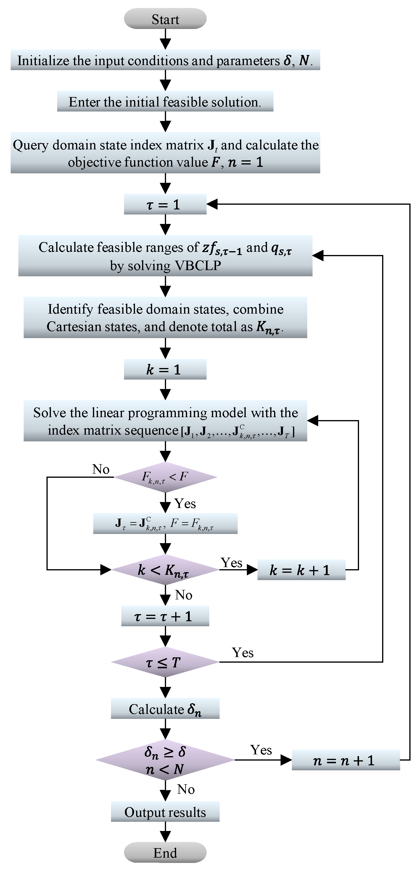
3.4. PLPOMDNF Solution Process

The PLPOMDNF solution flow is shown in Figure 6, and the solution process involves the following 12 steps:

• Initialize the input conditions of each hydropower station in the cascade and the parameters of the PLPOMDNF, including $\delta$ and $N$.
• Enter the initial feasible solution.
• Query the combinatorial domain state index matrix $J_t$, calculate the objective function value $F$ according to the initial feasible solution, and recode. Set $n=1$.
• Set the stage variable $\tau =1$.
• Calculate the feasible ranges of the initial water level $z{f}_{s,\tau -1}$ and power water release $q_{s,\tau }$ for each station in period $\tau$ by solving the VBCLP, which should be calculated $4S$ times.
• Identify the feasible domain state of each station and then combine all states in a Cartesian fashion, resulting in a total of $K_{n,\tau }$ states.
• Set $k=1$.
• The combinatorial domain state index matrix is $J_{k,n,\tau }^{\mathrm{C}}$ for periods $\tau$ and $J_t$ for other periods. Solve the linear programming model with the index matrix sequence $[J_1,J_2,\dots ,J_{k,n,\tau }^{\mathrm{C}},\dots ,J_T]$. If the new objective function $F_{k,n,\tau }$ is better, set $J_{\tau }=J_{k,n,\tau }^{\mathrm{C}}$ and $F=F_{k,n,\tau }$.
• If $k<K_{n,\tau }$, set $k=k+1$ and return to step 8; otherwise, go to step 10.
• Set $\tau =\tau +1$. If $\tau \le T$, return to step 5; otherwise, go to step 11.
• Calculate ${\delta }_n$. If ${\delta }_n\ge \delta$ and $n<N$, set $n=n+1$ and return to step 4; otherwise, go to step 12.
• End the calculation and output the result.

4. Case Study and Discussion

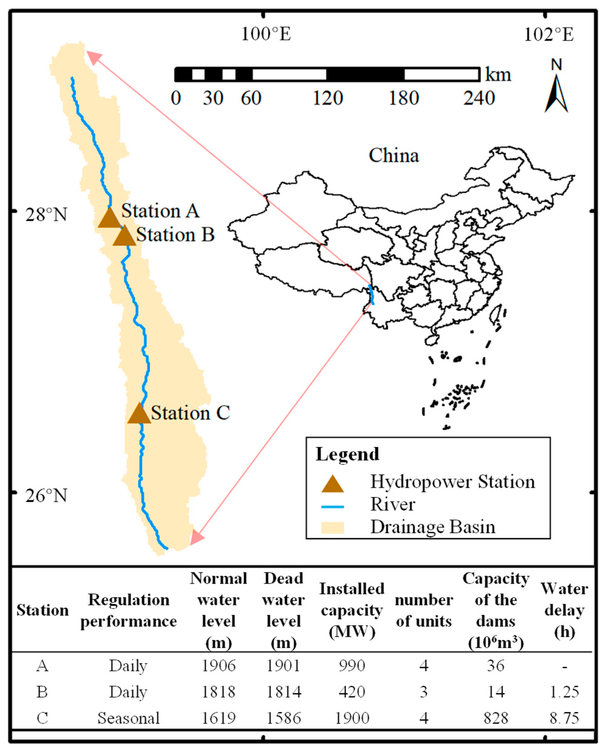
4.1. Introduction to Research Objects

In this study, we focused on simulating short-term optimal scheduling for three cascade hydropower stations, Station A, Station B, and Station C, located upstream of a large hydropower base in southwest China. This hydropower base plays a crucial role in supplying power to Yunnan Province and supporting the West–East electricity transmission project. The upstream stations have a substantial influence on the entire cascade operation due to their intricate hydraulic interconnections. However, the presence of complex nonlinear constraints and sensitive head variations poses challenges to refining operational strategies. Consequently, considerable untapped optimization potential remains within the current rudimentary short-term plans. Figure 7 depicts the cascade topology and pertinent information regarding the three cascade hydropower stations.

The scheduling cycle was 24 h, and the duration of one time period was 15 min. By solving the STOSCHS problem, a comparison between the PLPOMDNF and MILP was conducted to verify the convergence and accuracy of the PLPOMDNF. Both the POA and the PLPOMDNF adopted uniform power generation as the initial feasible solution. The water storage discretization step of the POA was 10,000 cubic meters, while the ZV function and ZQ function in MILP were approximated by three continuous line segments each; the PHQ function was approximated by a continuous space composed of eight triangular planes. To ensure the generalizability and robustness of the research, simulations were conducted using actual data from typical dry and wet season days. The algorithm is implemented in Python 3.9, and linear programming is solved using the Gurobi 9.1 solver [34].

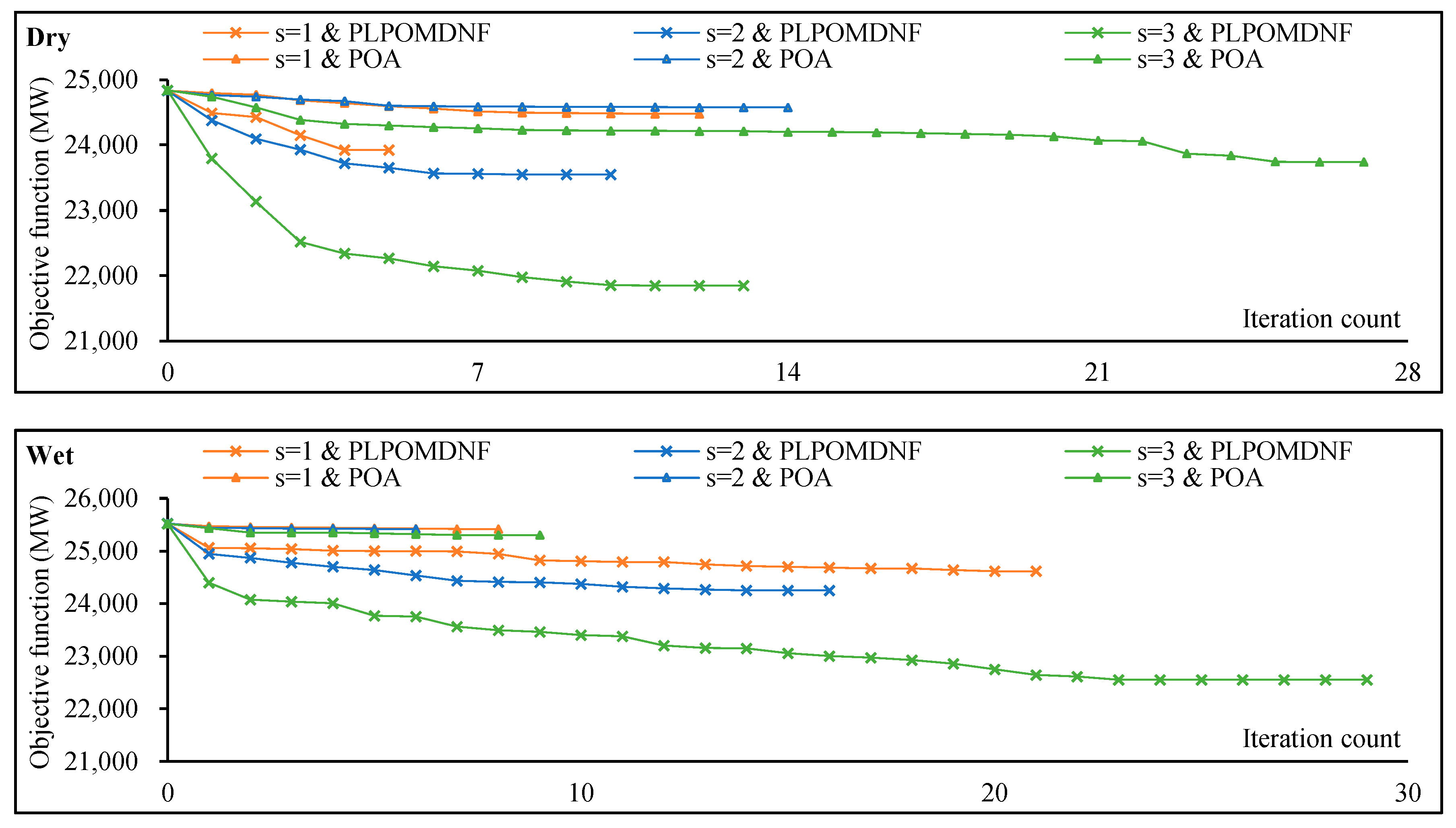
4.2. Comparison of Different Solution Methods

The various methods for addressing the STOSCHS issue at different scales during the dry and wet seasons are compared in this study, with

Table 1. Comparison of the results by different methods.

Season	Number of Stations	Method	Iteration Count	Peak–Valley Difference (MW)			Improvement of PLPOMDNF (MW)
				Original Load	Residual Load	Reduction
Dry	1	MILP	-	24,822	23,926	896	7
		POA	12		24,475	347	556
		PLPOMDNF	5		23,919	903	-
	2	MILP	-		23,557	1265	10
		POA	14		24,573	249	1026
		PLPOMDNF	10		23,547	1275	-
	3	MILP	-		22,462	2360	612
		POA	27		23,739	1083	1889
		PLPOMDNF	13		21,850	2972	-
Wet	1	MILP	-	25,520	24,625	895	8
		POA	8		25,418	102	801
		PLPOMDNF	21		24,617	903	-
	2	MILP	-		24,255	1265	8
		POA	6		25,420	100	1173
		PLPOMDNF	16		24,247	1273	-
	3	MILP	-		23,383	2137	521
		POA	9		25,301	219	2439
		PLPOMDNF	19		22,862	2658	-

presenting the computational results. Overall, the peak load shedding effectiveness of the PLPOMDNF surpasses that of both the POA and MILP. Specifically, during the dry and wet seasons, the PLPOMDNF caused the peak–valley differences at the three hydropower stations to decrease by 2972 MW and 2658 MW, respectively. During the dry season, the PLPOMDNF reduced the residual load peak–valley differences by 612 MW and 1889 MW compared to the MILP and POA, whereas during the wet season, these values are 521 MW and 2439 MW, respectively. These results occurred because although the MILP model theoretically offers the ability to compute the global optimum, the approximation errors resulting from the elimination of the nonlinear function relationships degrade the quality of the solutions. This phenomenon explains why the quality of MILP solutions deteriorates with an increase in the number of hydropower stations. The performance disparity between the PLPOMDNF and POA can be attributed to the tendency of the POA to prematurely converge to local optima under identical initial feasible solutions.

Based on the iteration count and objective function results in Table 1, the PLPOMDNF clearly requires fewer iterations during the dry season than the POA does, while more iterations are needed during the wet season. Furthermore, its objective function consistently outperforms that of the POA. Due to the abundant water supply during the wet season, it is difficult for hydropower stations to operate at lower outputs to avoid water waste. Therefore, the feasible domain during the wet season is usually limited, making the POA more prone to premature convergence to local optima. In contrast, the utilization of continuous domain states in PLPOMDNF enhances its convergence properties, facilitating escape from local optima. Despite the smaller feasible domain of variables in the wet season leading to a greater number of iterations, the PLPOMDNF still demonstrates remarkable convergence. To further validate the superior convergence of the PLPOMDNF, we examine the variations in the objective function values upon the completion of iterations during the dry and wet seasons for different numbers of hydropower stations, as shown in Figure 8. The results indicate that both the PLPOMDNF and POA exhibit a monotonic convergence trend; however, the PLPOMDNF demonstrates a faster convergence rate during the early iteration stages, often surpassing the final objective function value of the POA after just two iterations. This rapid convergence can be attributed to the application of domain states, which allow the station conditions to be adjusted during noncomputational periods to enhance the relationships between periods.

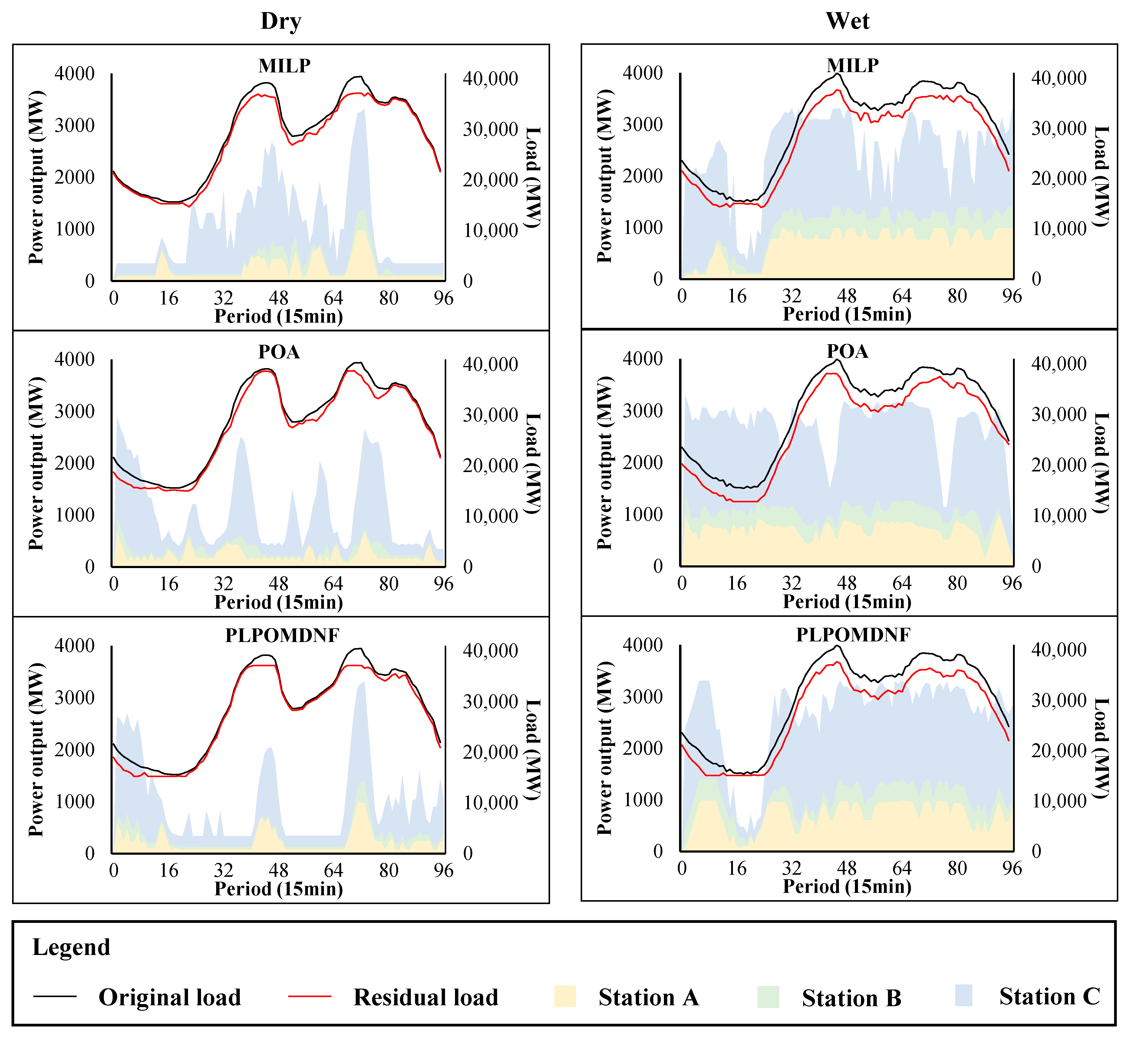
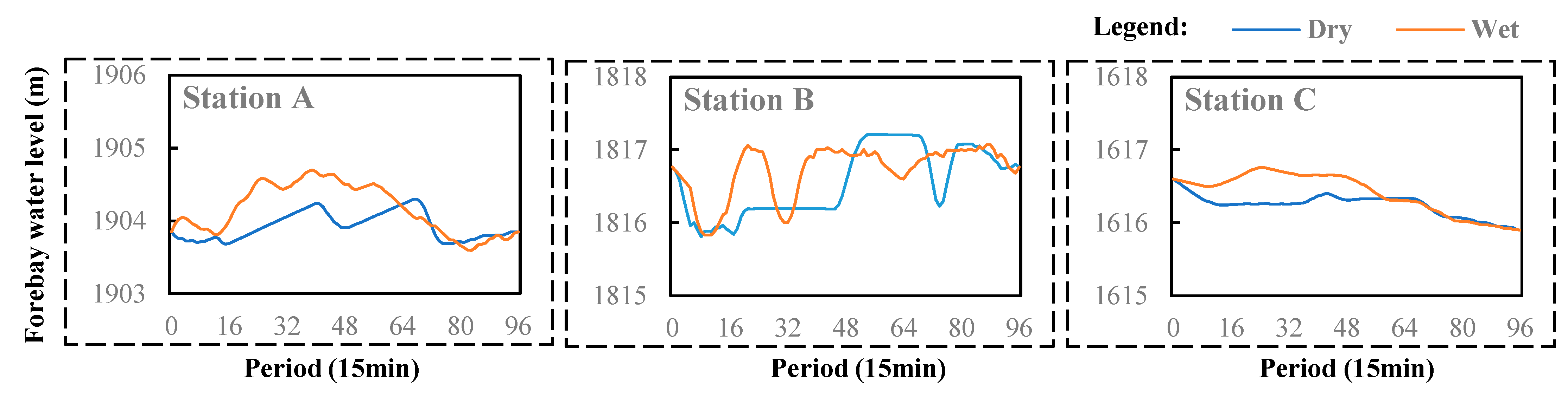
4.3. Analysis of Result Rationality

To validate the effectiveness of the proposed method for solving STOSCHS problems, the results for three hydropower stations on typical days during the wet and dry seasons are presented in Figure 9. Compared with the original load, the optimization results of each method consistently reduce the peak–valley difference in load during both the dry and wet seasons, enabling a smoother residual load profile throughout the cascade. Among these methods, the PLPOMDNF method results in the most favorable outcomes, reducing the peak–valley differences in load by 2972 MW and 2658 MW during the dry and wet seasons, respectively. Each station is capable of generating at maximum capacity during peak load periods, specifically the 73rd time period during the dry season and the 46th time period during the wet season, while operating at minimum available flow during valley load periods, namely the 19th time period during the dry season and the 19th time period during the wet season. This result demonstrates that the proposed PLPOMDNF method can effectively harness the peaking capabilities of the cascade during both the wet and dry seasons, adequately addressing the increased load peak demands under extreme climate conditions. In contrast, due to premature convergence, the POA method fails to operate at maximum and minimum capacities during peak and valley load periods, while the MILP approximation errors during peak and valley periods, such as the 23rd and 75th time periods during the dry season and the 24th time period during the wet season, adversely affect its peaking performance.

The residual load profiles during the wet and dry seasons of the PLPOMDNF exhibit distinct characteristics. During the wet season, a “valley filling” pattern is observed when the residual load is adjusted to form a linear curve during valley periods. Conversely, during the dry season, a “peak shaving and valley filling” pattern emerges, where the residual load is modulated into a linear curve during both the peak and valley periods. During the dry season, due to reduced water inflow, cascaded hydropower stations possess adequate regulation capacity to prioritize power generation during peak periods while conserving water during valley periods. However, during the wet season, with abundant water inflow and the need for reservoir regulation during valley periods, hydropower stations must operate at higher capacities during other periods to avoid water spillage. This phenomenon explains why the shape of the residual load during peak hours during the wet season remains largely similar to the original load profile. Overall, the PLPOMDNF is applicable across seasons, enabling the exploration of load regulation potential in cascaded hydropower stations to ensure the secure and stable operation of power grids.

Figure 10 illustrates the forebay water level variations during both the dry and wet seasons at each hydropower station. Clearly, the forebay water level fluctuations at these stations are substantial. Among them, the largest intraday fluctuation occurs during the dry season at Station B, reaching 1.40 m, while the smallest fluctuation occurs at Station A during the dry season, at 0.61 m. These significant forebay water level variations result in considerable changes in the water head and power water release throughout the scheduling cycle, underscoring the necessity for accurate modeling of the NLFs that describe these relationships.

To further illustrate the advantages of the proposed method in terms of accuracy, we compared the power output process calculated using PLPOMDNF, MILP, and POA based on typical daily actual operational water level data and compared the results with actual power output data. Figure 11 presents a comparison of the output results, with the POA method following the approach outlined in reference [28] and the MILP method based on the method described in reference [17]. It can be observed that the power output process obtained by PLPOMDNF and POA is identical and closely matches the actual process, with errors during both the wet and dry seasons being controlled within 5 MW. In contrast, MILP exhibits significant deviations, particularly during the dry season, where the maximum error reaches up to 34 MW. This is because PLPOMDNF performs feasible domain decomposition based on discrete points, which is essentially a piecewise linear interpolation of the nonlinear curve at discrete points. In the POA method, the complexity of the nonlinear function has minimal impact on the solution difficulty, so accurate piecewise linear interpolation is also used to describe the nonlinear function. Since MILP requires incorporating the entire nonlinear function into the model, using an accurate piecewise linear interpolation would introduce a large number of integer variables, making it impossible to complete the solution using a centralized approach. Therefore, as described in Reference [17], an approximation method is used to ensure the feasibility of the solution, which leads to a decrease in accuracy.

4.4. Effectiveness of the Dimensionality Reduction Strategy

The proposed dimensionality reduction strategy was employed to eliminate infeasible domain states of each hydropower station before proceeding with Cartesian combination. Figure 12 illustrates the combinatorial domain state quantity for the first iteration during the wet and dry seasons. Without the use of the dimensionality reduction strategy, the states at each stage would reach a formidable 66,355,200, which would be fatal to the efficiency of the STOSCHS regardless of the superior optimization capabilities of the PLPOMDNF. With the adoption of the feasible domain state dynamic acquisition method, the average number of combinatorial domain states sharply decreases to approximately 10,667 and 5485 during the wet and dry seasons, respectively, representing less than 0.02% of the original count. A further reduction in the combinatorial domain state quantity can be achieved by computing variable feasible ranges using the VBCLP. Particularly during wet seasons, due to significant natural inflows, the feasible range of power water release at each stage is often too small to prevent spillage, resulting in a greater proportion of infeasible domain states, thus leading to a more pronounced reduction in states during wet seasons. During the wet and dry seasons, the average state quantities decreased to 877 and 649, respectively, representing reductions of 91.8% and 88.2% from the original number of feasible combinatorial domain states, which indicates the effectiveness of the proposed dimensionality reduction strategy.

5. Conclusions

To address the substantial challenges posed to the power supply by extreme weather events and the large-scale integration of renewable energy sources, this paper proposes a PLPOMDNF to increase the accuracy and optimization depth of the STOSCHS. First, this method decomposes the entire feasible domain into a series of subdomains based on the characteristics of the NLFs to accurately depict nonlinearity and mitigate the difficulty of finding a solution. Then, by treating these continuous subdomains as states and integrating the progressive optimality principle suitable for solving multistage problems, a progressive linear programming optimality algorithm is subsequently designed to increase the convergence capability. Finally, to improve the computational efficiency, a dimensionality reduction strategy is employed to eliminate infeasible domain states before each stage, thereby avoiding unnecessary computations. A simulation using actual data from three hydropower stations in a river basin in southwest China during the dry and wet seasons revealed the following conclusions:

• Significant fluctuations in daily hydropower station forebay water levels introduce errors that cannot be ignored when approximating NLFs. Compared with the commonly used MILP, which introduces large integers for approximations of NLFs, coupling NLF characteristics with their decomposition prevents the introduction of errors and results in more precise outcomes. The power output errors during both the wet and dry seasons can be controlled within 5 MW.
• Compared with the common POA, the PLPOMDNF converges faster within a single iteration and achieves superior final objectives, indicating that the use of continuous domain states provides adjustability for non-optimization stages, ensuring strong convergence of the algorithm. Typically, after two iterations, the objective function value of PLPOMDNF surpasses the final objective function value of POA.
• The feasible domain state dynamic acquisition method using variable bounds obtained through the VBCLP successfully reduces the number of states in each stage, demonstrating that the proposed dimensionality reduction strategy lowers the solution complexity by avoiding unnecessary computations. The method reduces the number of domain states during the wet and dry seasons by 91.8% and 88.2%, respectively.

These results underscore that the PLPOMDNF enables more accurate and deeper optimization of the STOPSHS, providing robust support for electricity supply in power systems. Future work could further enhance the dimensionality reduction capabilities of the PLPOMDNF by integrating cascade decomposition strategies and parallel techniques to improve solution efficiency, thereby facilitating the management of large-scale hydropower short-term scheduling and improving the efficiency of water resource utilization. In addition, this study utilizes deterministic runoff data, while a more in-depth consideration of runoff uncertainty could potentially lead to more optimal solutions.

References

- Rosinska, W.; Jurasz, J.; Przestrzelska, K.; Wartalska, K.; Kazmierczak, B. Climate change’s ripple effect on water supply systems and the water-energy nexus—A review. Water Resour. Ind. 2024, 32, 100266. [Google Scholar] [CrossRef]
- Perera, A.T.D.; Nik, V.M.; Chen, D.L.; Scartezzini, J.L.; Hong, T.Z. Quantifying the impacts of climate change and extreme climate events on energy systems. Nat. Energy 2020, 5, 150–159. [Google Scholar] [CrossRef]
- Bhatti, B.A.; Hanif, S.; Alam, J.; Mitra, B.; Kini, R.; Wu, D. Using energy storage systems to extend the life of hydropower plants. Appl. Energy 2023, 337, 120894. [Google Scholar] [CrossRef]
- Sterl, S.; Vanderkelen, I.; Chawanda, C.J.; Russo, D.; Brecha, R.J.; van Griensven, A.; van Lipzig, N.P.M.; Thiery, W. Smart renewable electricity portfolios in West Africa. Nat. Sustain. 2020, 3, 710–719. [Google Scholar] [CrossRef]
- Wan, W.H.; Wang, H.; Zhao, J.S. Hydraulic Potential Energy Model for Hydropower Operation in Mixed Reservoir Systems. Water Resour. Res. 2020, 56, e2019WR026062. [Google Scholar] [CrossRef]
- Jamali, S.; Jamali, B. Cascade hydropower systems optimal operation: Implications for Iran’s Great Karun hydropower systems. Appl. Water Sci. 2019, 9, 66. [Google Scholar] [CrossRef]
- Li, X.; Wei, J.H.; Li, T.J.; Wang, G.Q.; Yeh, W.W.G. A parallel dynamic programming algorithm for multi-reservoir system optimization. Adv. Water Resour. 2014, 67, 1–15. [Google Scholar] [CrossRef]
- Zhao, T.T.G.; Zhao, J.S.; Yang, D.W. Improved Dynamic Programming for Hydropower Reservoir Operation. J. Water Resour. Plan. Manag. 2014, 140, 365–374. [Google Scholar] [CrossRef]
- Zhao, Q.K.; Cai, X.M.; Li, Y. Algorithm Design Based on Derived Operation Rules for a System of Reservoirs in Parallel. J. Water Resour. Plan. Manag. 2020, 146, 5. [Google Scholar] [CrossRef]
- Jia, Z.B.; Shen, J.J.; Cheng, C.T.; Zhang, Y.; Lyu, Q. Optimum day-ahead clearing for high proportion hydropower market considering complex hydraulic connection. Int. J. Electr. Power Energy Syst. 2022, 141, 108211. [Google Scholar] [CrossRef]
- Liao, S.L.; Liu, Z.W.; Liu, B.X.; Wu, X.Y.; Cheng, C.T.; Su, H.Y. Short-Term Hydro Scheduling Considering Multiple Units Sharing a Common Tunnel and Crossing Vibration Zones Constraints. J. Water Resour. Plan. Manag. 2021, 147, 10. [Google Scholar] [CrossRef]
- Liu, B.X.; Lund, J.R.; Liao, S.L.; Jin, X.Y.; Liu, L.J.; Cheng, C.T. Optimal power peak shaving using hydropower to complement wind and solar power uncertainty. Energy Convers. Manag. 2020, 209, 112628. [Google Scholar] [CrossRef]
- Lima, R.M.; Marcovecchio, M.G.; Novais, A.Q.; Grossmann, I.E. On the Computational Studies of Deterministic Global Optimization of Head Dependent Short-Term Hydro Scheduling. IEEE Trans. Power Syst. 2013, 28, 4336–4347. [Google Scholar] [CrossRef]
- Shen, J.J.; Chen, G.Z.; Cheng, C.T.; Wei, W.; Zhang, X.F.; Zhang, J. Modeling of Generation Scheduling for Multiple Provincial Power Grids Using Peak-Shaving Indexes. J. Water Resour. Plan. Manag. 2021, 147, 9. [Google Scholar] [CrossRef]
- Wang, J.; Cheng, C.T.; Shen, J.J.; Cao, R.; Yeh, W.W.G. Optimization of Large-Scale Daily Hydrothermal System Operations with Multiple Objectives. Water Resour. Res. 2018, 54, 2834–2850. [Google Scholar] [CrossRef]
- Cheng, C.T.; Wang, J.Y.; Wu, X.Y. Hydro Unit Commitment With a Head-Sensitive Reservoir and Multiple Vibration Zones Using MILP. IEEE Trans. Power Syst. 2016, 31, 4842–4852. [Google Scholar] [CrossRef]
- Fang, Z.; Liao, S.L.; Zhao, H.Y.; Cheng, C.T.; Liu, B.X.; Wang, H.; Li, S.S. An MILP model based on a processing strategy of complex multisource constraints for the short-term peak shaving operation of large-scale cascaded hydropower plants. Renew. Energy 2024, 231, 120932. [Google Scholar] [CrossRef]
- Su, C.G.; Wang, P.L.; Yuan, W.L.; Cheng, C.T.; Zhang, T.H.; Yan, D.H.; Wu, Z.N. An MILP based optimization model for reservoir flood control operation considering spillway gate scheduling. J. Hydrol. 2022, 613, 128483. [Google Scholar] [CrossRef]
- Teegavarapu, R.S.V.; Ferreira, A.R.; Simonovic, S.P. Fuzzy multiobjective models for optimal operation of a hydropower system. Water Resour. Res. 2013, 49, 3180–3193. [Google Scholar] [CrossRef]
- Wu, X.; Shen, X.J.; Wei, C.J.; Xie, X.M.; Li, J.S. A Hybrid Particle Swarm Optimization-Genetic Algorithm for Multiobjective Reservoir Ecological Dispatching. Water Resour. Manag. 2024, 38, 2229–2249. [Google Scholar] [CrossRef]
- Qiu, R.J.; Wang, D.; Singh, V.P.; Wang, Y.K.; Wu, J.C. Integration of deep learning and improved multi-objective algorithm to optimize reservoir operation for balancing human and downstream ecological needs. Water Res. 2024, 253, 121314. [Google Scholar] [CrossRef] [PubMed]
- Azizipour, M.; Ghalenoei, V.; Afshar, M.H.; Solis, S.S. Optimal Operation of Hydropower Reservoir Systems Using Weed Optimization Algorithm. Water Resour. Manag. 2016, 30, 3995–4009. [Google Scholar] [CrossRef]
- Azizipour, M.; Sattari, A.; Afshar, M.H.; Goharian, E. Incorporating reliability into the optimal design of multi-hydropower systems: A cellular automata-based approach. J. Hydrol. 2022, 604, 127227. [Google Scholar] [CrossRef]
- Zhao, T.T.G.; Cai, X.M.; Lei, X.H.; Wang, H. Improved Dynamic Programming for Reservoir Operation Optimization with a Concave Objective Function. J. Water Resour. Plan. Manag. 2012, 138, 590–596. [Google Scholar] [CrossRef]
- Chai, F.X.; Peng, F.; Zhang, H.P.; Zang, W.B. Stable Improved Dynamic Programming Method: An Efficient and Accurate Method for Optimization of Reservoir Flood Control Operation. Water Resour. Manag. 2023, 37, 5635–5654. [Google Scholar] [CrossRef]
- Feng, Z.K.; Niu, W.J.; Cheng, C.T.; Liao, S.L. Hydropower system operation optimization by discrete differential dynamic programming based on orthogonal experiment design. Energy 2017, 126, 720–732. [Google Scholar] [CrossRef]
- Fang, Z.; Liao, S.L.; Cheng, C.T.; Zhao, H.Y.; Liu, B.X.; Su, H.Y. Parallel improved DPSA algorithm for medium-term optimal scheduling of large-scale cascade hydropower plants. Renew. Energy 2023, 210, 134–147. [Google Scholar] [CrossRef]
- Feng, Z.K.; Niu, W.J.; Cheng, C.T.; Wu, X.Y. Peak operation of hydropower system with parallel technique and progressive optimality algorithm. Int. J. Electr. Power Energy Syst. 2018, 94, 267–275. [Google Scholar] [CrossRef]
- Liao, S.L.; Liu, H.; Liu, B.X.; Liu, T.; Li, C.H.; Su, H.Y. Solution framework for short-term cascade hydropower system optimization operations based on the load decomposition strategy. Energy 2023, 277, 127685. [Google Scholar] [CrossRef]
- Zhao, H.Y.; Liao, S.L.; Fang, Z.; Liu, B.X.; Ma, X.Y.; Lu, J. Short-term peak-shaving operation of “N-reservoirs and multicascade” large-scale hydropower systems based on a decomposition-iteration strategy. Energy 2024, 288, 129834. [Google Scholar] [CrossRef]
- Cheng, C.T.; Wang, S.; Chau, K.W.; Wu, X.Y. Parallel discrete differential dynamic programming for multireservoir operation. Environ. Model. Softw. 2014, 57, 152–164. [Google Scholar] [CrossRef]
- Liu, P.; Cai, X.M.; Guo, S.L. Deriving multiple near-optimal solutions to deterministic reservoir operation problems. Water Resour. Res. 2011, 47, W08506. [Google Scholar] [CrossRef]
- Feng, Z.K.; Niu, W.J.; Cheng, C.T. China’s large-scale hydropower system: Operation characteristics, modeling challenge and dimensionality reduction possibilities. Renew. Energy 2019, 136, 805–818. [Google Scholar] [CrossRef]
- Optimization Gurobi. Gurobi Optimizer Reference Manual. 2020. Available online: http://www.gurobi.com (accessed on 1 December 2020).