Evaluation of Water Richness in Sandstone Aquifers Based on the CRITIC-TOPSIS Method: A Case Study of the Guojiawan Coal Mine in Fugu Mining Area, Shaanxi Province, China

Abstract

Taking the Guojiawan coal mine in the Shenfu Mining Area as a case study, five evaluation factors (aquifer thickness, brittle–plastic rock thickness ratio, core recovery rate, number of sandstone–mudstone interbeds, and fractal dimension of the faults) were selected as indicators to evaluate the water richness of the sandstone aquifer in the roof strata of the main coal seam. Accordingly, the weights of the water richness evaluation indicators, derived using the criteria importance through intercriteria correlation (CRITIC) evaluation method, were integrated with the computational procedures of the technique for order of preference by similarity to ideal solution (TOPSIS) evaluation method. The indicator weights and evaluation approaches were combined through different fusion strategies. Finally, based on the water richness zoning results for the study area, the advantages and disadvantages of the two fusion approaches, C-TOPSIS-a and C-TOPSIS-b, were compared. Comprehensive analysis was conducted to evaluate the rationality of the water richness zoning. The C-TOPSIS-b evaluation method achieved the optimal evaluation outcome. The water richness was classified into five grades: weak, relatively weak, moderate, relatively strong, and strong. Among these, the regions with weak to relatively weak, moderate, and strong to relatively strong water richness are primarily in the northern, central, southern, and southwestern parts, respectively.

1. Introduction

Roof water represents the second most significant hazard source, following coalbed methane. The geographical distribution of roof water hazard incidents is closely correlated with the coal production capacity, thus exerting a substantial impact on coal resource exploitation [1,2]. After coal mining, water-conducting fissures are formed in the roof rock layer under the influence of mining, and if the fissures are connected to water-rich aquifers, the water in the aquifers will pour into the mine through the fissure channels, threatening the safety of operators and the normal operation of equipment [3,4]. The primary risk of the roof slab lies in the water breakout and roof slab instability caused by the joint action of the water filling source and fissure channel. Therefore, scientific evaluation of the water-rich nature of the aquifer overlying the roof of the coal seam and the formulation of targeted prevention and control measures are key to ensuring the safe and efficient mining of the coal seam.

Scholars have conducted numerous studies on aquifer water enrichment. Cheng Jiulong et al. [5] conducted simulations and on-site mine transient electromagnetic tests for water richness prediction using the bat optimization algorithm and neural network and realized quantitative prediction of the water richness of the rock formation. Hou E.K. et al. [6,7,8] used the whale optimization algorithm-support vector machine discriminant model to predict the water richness level of the weathered bedrock in the area without pumping test data to realize water richness zoning. The prediction results are in good agreement with the actual situation. The analytic hierarchy process (AHP) method and other subjective assignment methods have been widely used in aquifer water richness evaluation [9,10,11]. Fang G. [12] utilized the ArcGIS software and hierarchical analysis method to predict the water richness of the No.2 coal seam in the study area. Lyu Z.M. et al. [13] utilized the hierarchical analysis method to establish a water richness evaluation model of the Austrian ash, and their results fit with the geological conditions of the study area. Sun K. et al. [14] used hierarchical analysis to calculate the weights of each water richness index to obtain the distribution of the water richness index in the lower section of the Zhi Luo Formation. However, the subjective assignment method has a high degree of human subjectivity, leading to a lack of objectivity in the determination of the weights due to human interpretation reasons. In determining the weights of the indicators for water enrichment evaluation, the objective weighting method takes into account both the variability among the data to be evaluated and the correlation between the data. The entropy weight method and coefficient of variation method for determining the weights of water richness evaluation indexes only take into account the variability of the data, and using a single method lacks a certain persuasive power. Therefore, the combined assignment method is currently the most widely used in water richness evaluation [15,16]. Yang L. et al. [17] used fuzzy AHP (FAHP) analysis and the coefficient of variation (CV) objective assignment method to assign the weights of water richness indicators and constructed a water richness evaluation model with the technique for order of preference by similarity to ideal solution (TOPSIS) sorting and rank sum ratio (RSR) assisted grading. Bai Y. et al. [18] used the fuzzy hierarchical analysis method and coefficient of variation method to comprehensively assign weights to evaluate the water richness of the weathered bedrock aquifer in the Nanliang coal mine. Liang G.L. et al. [19] used hierarchical analysis and the criteria importance through intercriteria correlation (CRITIC) method to calculate the weights and solved the comprehensive weights, based on which they carried out water richness zoning and evaluation. The combined assignment method is a mature application, which mainly uses a combination of the weights of the two evaluation methods to solve the problem. However, the water richness of the sandstone aquifer predicted in the combined weights solution is not accurate. There is not enough richness in the combination of methods and there is a lack of comparisons between different combinations. Thus, further research on the construction of evaluation models is needed.

The Yanan Formation is a sandstone aquifer. Following extraction of the No. 5-1 coal seam, the confining pressure in the roof strata increased. Analysis of the effect of the confining pressure and the mechanisms of sandstone failure revealed that the sandstone exhibits abrupt failure characteristics under these conditions [20]. Under the influence of mining activities, stress–strain relationships induce pore deformation in rocks and fracture development within the rock mass, leading to changes in the permeability. These fractures connect overlying aquifers, thereby triggering mine water inrush disasters [21,22]. Based on this, in this study, the CRITIC-TOPSIS method was selected to evaluate the water richness of the Yanan Formation sandstone aquifer overlying the No. 5-1 coal seam. The CRITIC-TOPSIS method solves the deficiencies of traditional methods in terms of weight subjectivity and redundant processing of indicators through combination of objective assignment and dynamic closeness ranking. Compared with methods that require complex optimization, the calculation results of this method are transparent and it is easy to retrace the influences of key indicators, which enhances the reliability of the results in terms of the geological significance.

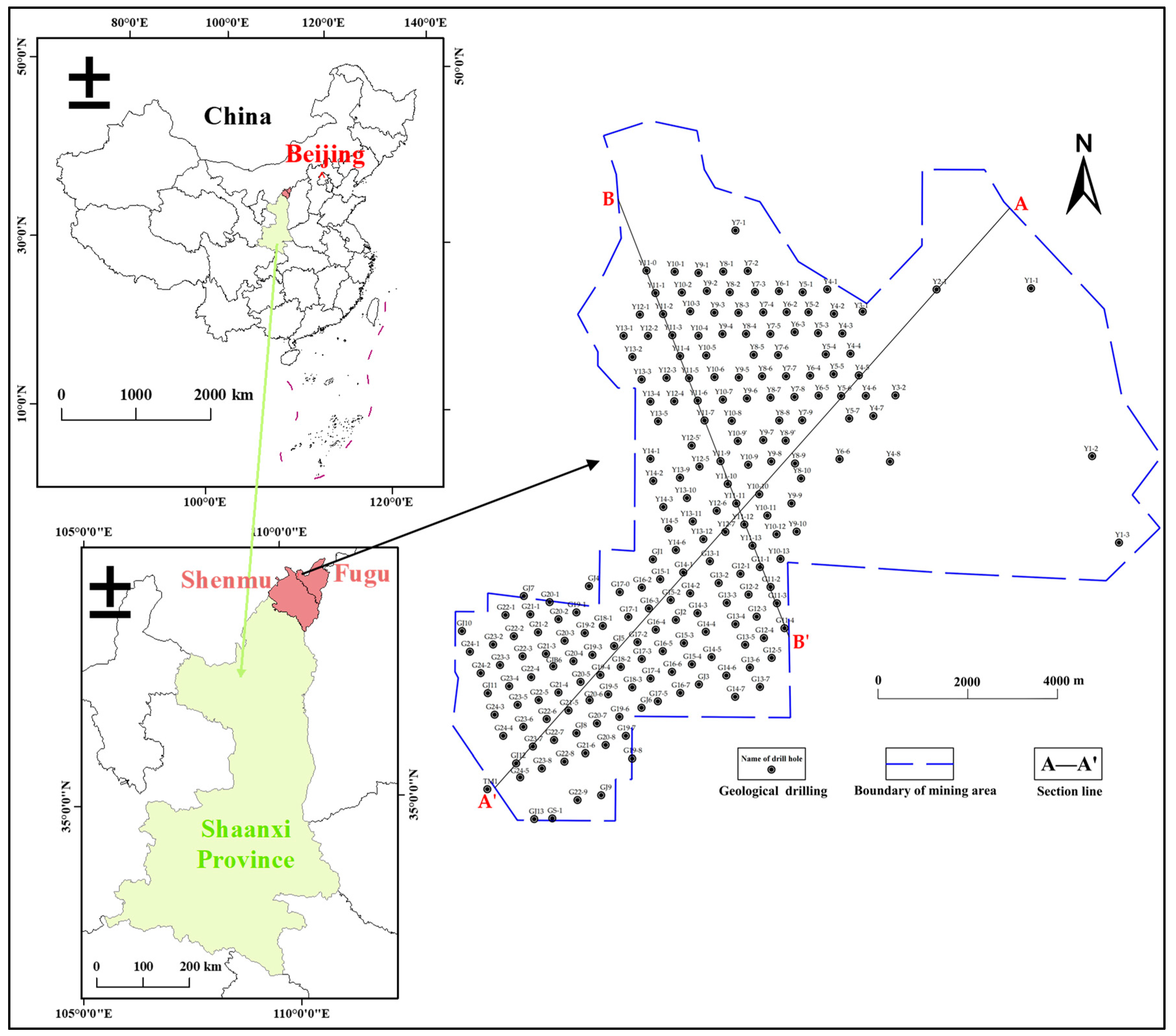
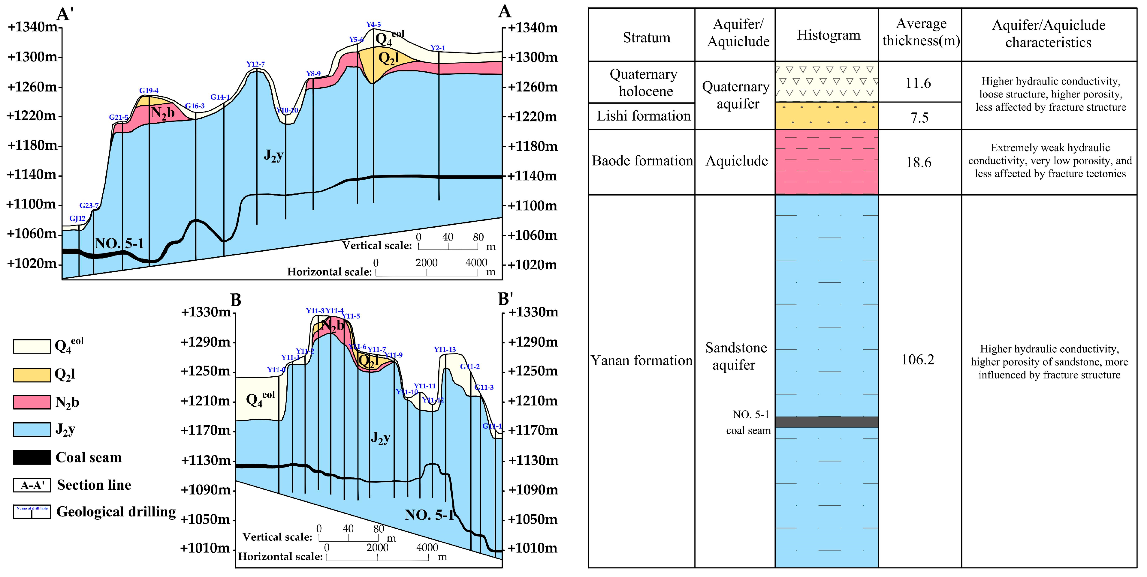
2. Overview of the Study Area

The Guojiawan coal mine is located in the Yushenfu mining area, which is the largest coal base in the Jurassic coalfield in northern Shaanxi, in the northern Ordos Basin. Deposition in a variety of mud–carbon depositional environments resulted in the formation of a stable and continuous thick coal seam (Figure 1) [23,24]. The main coal-bearing stratum in Guojiawan is the Yanan Formation in the Middle Jurassic system, and the main coal seam being mined at present is the No. 5-1 coal seam. It is 0.25–9.78 m thick, and has burial depths of 10–204 m. Measurement results have revealed that the development height of the water-conducting fissure zone after mining ranges from 26.88 to 328.61 m, with an average of 96.09 m, and it has the potential to spread to the aquifer at the surface and the Yanan Formation aquifer in some areas, which will pose a direct water-filling threat to safe mining of the No. 5-1 coal seam.

The water-bearing layer overlying the No. 5-1 coal seam in the study area is the water-bearing sandstone layer in the Yanan Formation, which has a strong water-bearing capacity. The Baode Formation is a red clay aquifer with a weak water-bearing capacity. The loess pore aquifer in the Middle Pleistocene Lishi Formation has a weak water-bearing capacity. The Holocene floodplain aquifer has a weak water-bearing capacity (Figure 2). In general, the terrain in the study area is low in the south and high in the north, and the aquifer water flows from north to south. The aquifer in the Quaternary system mainly receives recharge from precipitation, and there is a complementary relationship with the surface water. The outcrop area of the sandstone aquifer in the Yanan Formation receives recharge from precipitation, and part of it receives recharge from the aquifer in the Quaternary system.

The main lithologies of the Yanan Formation aquifer in the study area are siltstone, fine-grained sandstone, medium-grained sandstone, mudstone, and coal seams. Among them, the sandstone is the water-bearing layer, the mudstone is the relative water-insulating layer, and the water-bearing and water-insulating layers are inter-distributed to form a composite aquifer group. The unit water influx of this aquifer (q) ranges from 0.00026 to 0.0437 L/sm. Due to the long-term weathering and erosion of the Yanan Formation and the influence of the depositional environment, the thickness of the sandstone varies greatly, and the spatial distribution of this aquifer is complicated. The aquifer in the Yanan Formation serves as a direct water source for the No. 5-1 coal seam and thus poses a greater threat to the production safety of the coal mine.

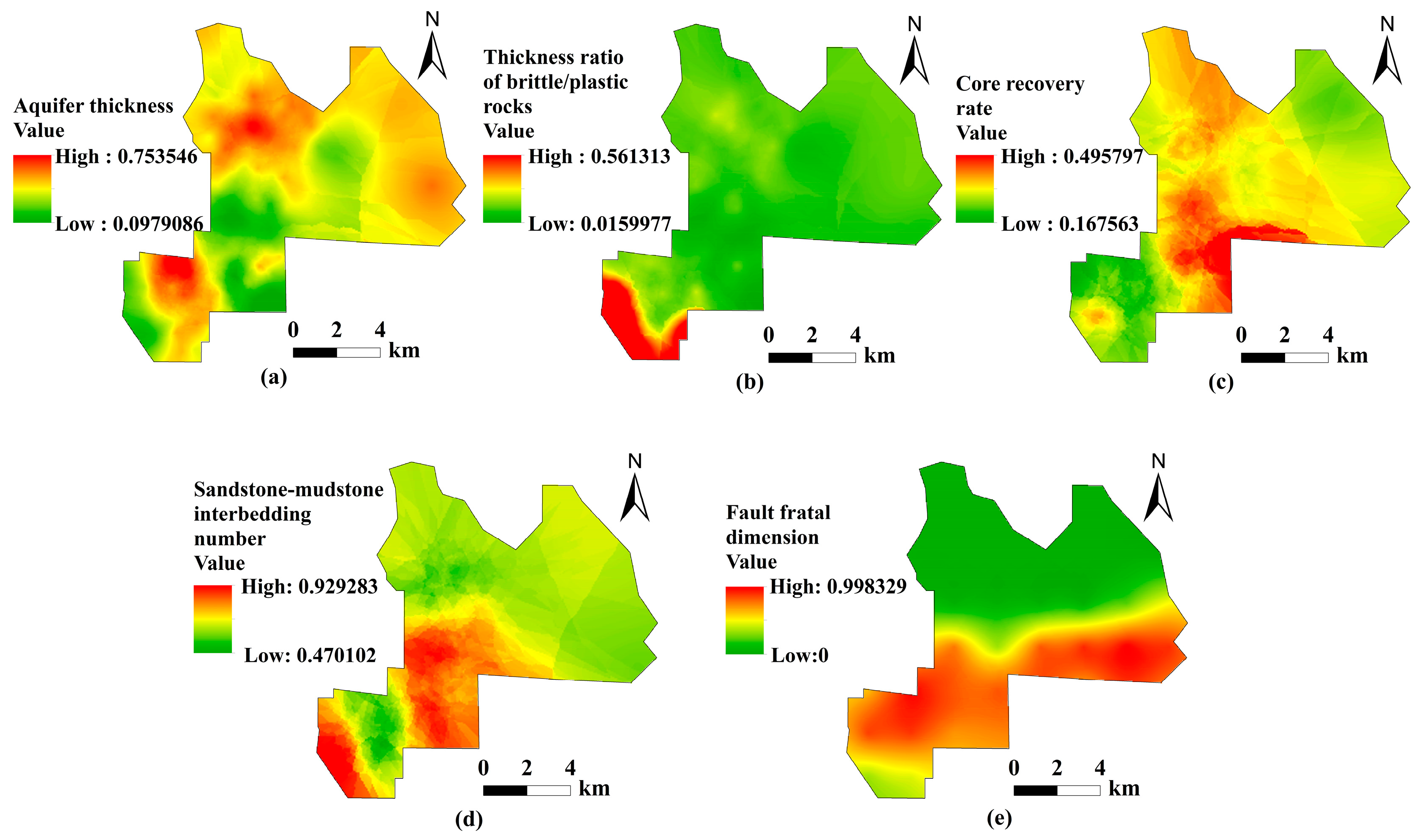
3. Evaluation Indicators

The water richness in the study area is affected by many factors, and the main factors controlling the water richness of the coal seam roof need to be appropriately selected to establish a reasonable water richness model as well as improve the accuracy of the evaluation results. Using borehole data and the characteristics of the tectonic development, the three major aspects (i.e., the lithology, hydraulic characteristics, and tectonic factors) were studied, and five indicators (i.e., the aquifer thickness, brittle–plastic rock thickness ratio, core recovery rate, number of sandstone–mudstone interlayers, and fault dimension value) were selected to conduct comprehensive analysis to serve as the main controlling factors for evaluating the water richness of the roof plate of the main mining coal seam (

Table 1. Statistics of each water richness evaluation indicator.

Serial Number	Drill Hole Number	Aquifer Thickness (m)	Thickness Ratio of Brittle/Plastic Rocks	Core Take Rate (%)	Number of Sandstone–Mudstone Interbeds	Fault Dimension
1	G11-1	21.43	0.14	73.02	12	1.10
2	G11-2	26.95	0.18	73.41	14	1.20
3	G11-3	90.75	1.01	54.77	7	1.25
4	G11-4	42.07	0.60	89.25	18	1.25
5	G12-1	33.40	0.21	89.74	25	1.15
6	G12-2	64.06	0.41	83.05	12	1.20
7	G12-3	61.92	0.44	79.89	24	1.25
8	G12-4	19.07	0.19	86.64	20	1.20
9	G12-5	36.52	0.33	74.76	19	1.20
10	G13-1	28.71	0.25	81.89	8	1.15
11	G13-2	44.64	0.31	89.59	25	1.20
12	G13-3	34.93	0.31	82.81	11	1.20
13	G13-4	107.07	2.28	82.03	12	1.20
14	G13-5	55.10	0.38	88.80	22	1.20
15	G13-6	16.17	0.31	85.90	10	1.15
17	G14-1	46.50	0.36	74.20	21	1.25
18	G14-2	58.90	0.44	71.72	11	1.25
19	G14-3	16.41	0.13	76.29	11	1.25
20	G14-4	20.30	0.16	73.49	7	1.25
…	…	…	…	…	…	…
195	Y11-3	89.63	1.14	88.08	29	0.00
196	Y11-4	79.07	0.76	81.25	18	0.00
197	Y11-5	70.56	0.69	93.75	20	0.00
198	Y11-6	58.94	0.72	81.32	24	0.00
199	Y11-7	34.45	0.59	87.65	17	0.05
200	Y12-1	86.40	1.08	87.70	18	0.00
201	Y12-2	60.43	0.62	83.98	30	0.00
202	Y12-3	94.50	1.27	79.35	35	0.00
203	Y12-4	68.51	0.98	88.36	22	0.00
204	Y12-5	41.26	0.55	84.04	18	0.55
205	Y13-1	68.71	0.73	89.28	22	0.00
206	Y13-2	27.62	1.01	91.07	10	0.00
207	Y13-3	48.49	0.43	83.37	20	0.00
208	Y13-4	79.99	1.08	86.72	31	0.00
209	Y13-5	70.14	1.20	83.19	34	0.10
210	Y14-1	66.15	1.66	92.40	19	0.50
211	GS-1	67.56	1.32	87.71	22	0.50
212	Y11-0	31.75	1.18	90.01	9	0.00

).

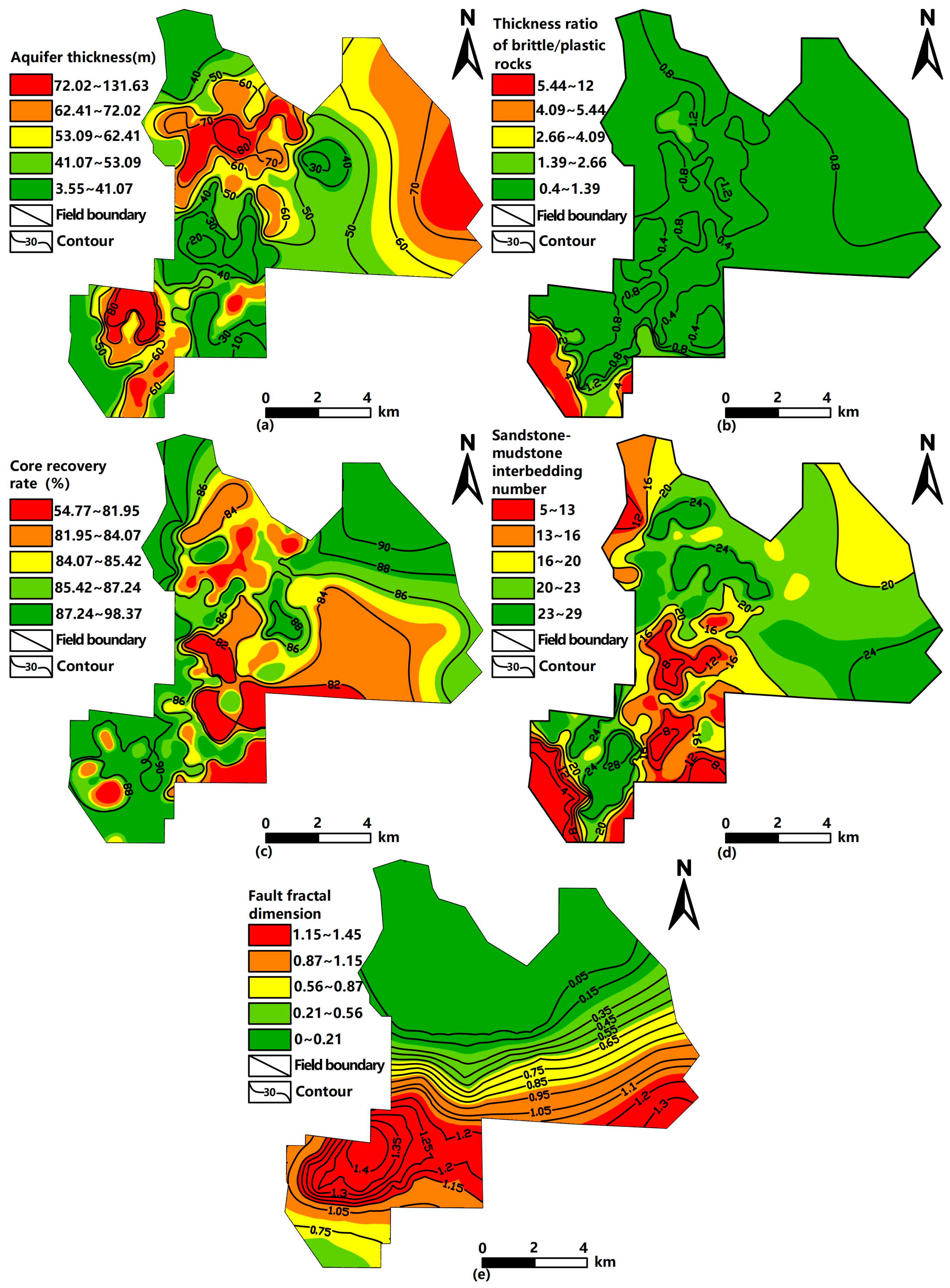
3.1. Sandstone Aquifer Thickness

The thickness of the sandstone aquifer can represent the size of the aquifer water storage space, is the premise of judging the strength of the water-rich nature of the rock section, and is also the most intuitive factor representing the water-rich nature of the aquifer. When all of the other factors are held constant, the thicker the sandstone aquifer is, the greater the water storage space per unit thickness of the sandstone is, and the more water-rich it is [25]. Therefore, the aquifer thickness is positively correlated with the water richness. The thickness of the aquifer to be evaluated is the total thickness of the water-bearing sandstone in the Yanan Formation in the top plate of the coal seam, and the thickness of the sandstone ranges from 3.55 to 131.63 m, with an average thickness of 54.59 m (Figure 3a).

3.2. Thickness Ratio of Brittle/Plastic Rocks

Due to the tectonic stresses, the brittle rocks are mainly sheared and under tensile stress, and the plastic rocks are primarily plastically deformed under stress. Brittle rocks refer to lithologies such as sandstone and conglomerate. For the brittle rock body, after deformation by a force, the pores and fissures are more developed, the formation of the water-conducting channels is enhanced, the permeability of the rock layer is greater, and it is a good aquifer water storage space. Plastic rocks refer to lithologies such as siltstone and mudstone. Compared to the brittle rocks, after deformation by a force, the permeability of the rock layer changes less, pores and fissures arenot developed, and the water permeability is weak. Compared to plastic rocks, brittle rocks are more likely to produce a large number of cracks under stress, which greatly increases their permeability and water storage capacity [26]. The greater the ratio of the thickness of the brittle rocks to the thickness of the plastic rocks in the aquifer is, the higher the percentage of the brittle rock type is, and the stronger the water-rich nature is, and vice versa, the weaker the water-rich nature is. Therefore, the thickness ratio of the brittle and plastic rocks is positively correlated with the water richness. The thickness ratio of the brittle and plastic rocks varies from 0 to 1.5 in most parts of the wellfield (Figure 3b).

3.3. Core Recovery Rate

The core recovery rate is an indicator of the rock quality. It is defined as the ratio of the total length of the rock layer recovered by drilling the core to the corresponding actual drilling footage in the same drilling return footage, reflecting to a certain extent the degree of rock integrity. The lower the core recovery rate is, the more complex the top plate structure is, the poorer the stability is, the more broken the rock is, the poorer the integrity is, the better the connectivity is, the better the permeability and water storage capacity are, the richer the water-rich space is, and the stronger the water-rich nature of the aquifer is [27]. Therefore, there is a negative correlation between the core recovery rate and the water richness. The core recovery rate of the entire study area is 74–94% (Figure 3c).

3.4. Number of Sandstone–Mudstone Interbeds

The number of sandstone–mudstone interbeds reflects the hydraulic connection between the aquifers, and the mudstones can form a watertight layer, which divides the aquifer to a certain extent and hinders the vertical hydraulic connection of the aquifer. The more sandstone–mudstone interlayers there are, the more difficult it is for water to flow within the aquifer, the less permeable the aquifer is, and the lower the water richness is. The fewer sandstone–mudstone interbeds there are, the easier it is for water to flow within the aquifer, and the higher the permeability is, resulting in endanced vertical hydraulic connection to the aquifer [28]. Therefore, the number of sandstone interbeds is negatively correlated with the water richness. The number of sandstone interbeds is more evenly distributed (Figure 3d).

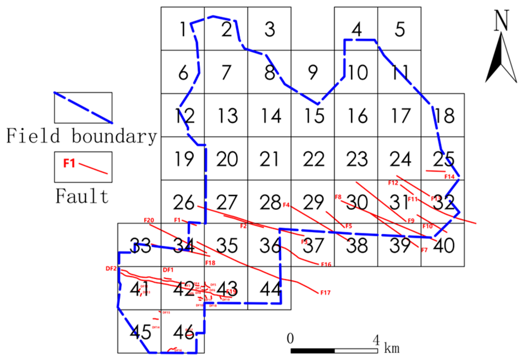
3.5. Fault Dimension

The theory of fractal ideas, first proposed by French mathematician Mandelbrot in the 1970s, is a nonlinear science that studies the objective irregularities and complexities that exist in nature [29,30]. It spans the natural, social, and thinking sciences and uses a unique sub-dimensional perspective and mathematical approach to reveal regularities and hierarchies in natural phenomena [31]. Faults have fractal structural characteristics, and the fractal dimension of faults, as a quantitative parameter, can accurately reflect the complexity of the rupture structure.

In this paper, the box dimension method is used, and the specific method steps are to cover the fixed scale wellfield area with a square grid of side length r = 2 km, divide the wellfield into 46 blocks, and count the number of square grids containing faults N(r). Varying the size of the grid side length r, square grids with r, r/2, r/4, and r/8 are utilized, and the number of square grids N(r) that have fault traces passing through them in the corresponding block section are counted. The relationship between the number of grids N(r) and the division of the square grid r by the corresponding level is such that N(r) and r satisfy the following power law relationship:

$$N(r)=a\cdot r^{-D_S}$$

(1)

where N(r) is the total number of faults intersecting the grid, a is a constant, D_s is the fault dimension, and r is the side length of the square grid.

The logarithms of both sides of Equation (1) are taken, a scatter plot of lgr versus lgN(r) is plotted, and the linear relationship (Equation (2)) of lgr–lgN(r) is solved for using the least-squares fitting method to obtain the dimension value of each block, Ds, and its correlation coefficient, R². The results of the calculation of the dimension values of each grid fault are presented in

Table 2. Fault sub-dimensional value statistics for the Guojiawan coal mine.

Grid Number	DS	R2	Grid Number	DS	R2
25	0.7551	0.9884	36	1.2721	0.9597
26	0.834	0.9902	37	1.317	0.9608
27	1.17	0.9974	39	1.3485	0.9965
29	1.2686	0.9927	40	1.0832	0.9937
30	1.4066	0.9713	41	1.3432	0.9668
31	1.5561	0.9878	42	1.3732	0.9974
32	1.3925	0.9955	43	1.0793	0.959
33	0.9422	0.9975	44	1.1288	0.9968
34	1.5214	0.9836	46	0.6585	0.9608
35	1.2686	0.9927

.

$$\lg N(r)=\lg a-D_s\lg r$$

(2)

where lgN(r) is the number of square grids through which the logarithmically transformed fault trace passes, lga is a logarithmically transformed constant, and lgr is the logarithmically varying grid edge length.

In this study, the box-counting method was employed to determine the fractal dimension value (D_s) of the studied fault. Grid partitioning was performed (Figure 4), and a regression curve of lgN(r) versus lgr was plotted (Figure 5). As shown in Table 1, the representative fractal dimension values of the block segments range from 0.6585 to 1.5561, with correlation coefficients ranging from 0.959 to 0.9975. This indicates that the faults in the Guojiawan coal mine exhibit strong self-similarity and fractal characteristics. The complexity of the faults exhibits a strong linear relationship with the magnitude of the fractal dimension values. The varying fractal dimension values of the different faults indicate differences in their development characteristics. Generally, the larger the fractal dimension value is, the more complex the fault structure is, the higher the degree of fragmentation in its development is, and the stronger its water-bearing capacity is. The smaller the fractal dimension value is, the simpler the fault structure is, and the weaker its water-bearing capacity is. Therefore, the fractal dimension value of a fault is positively correlated with its water-bearing capacity.

The central point coordinates of each block segment were interpolated with their corresponding fault fractal dimension values using software, resulting in the creation of a contour map of the fractal dimension values of the faults in the Guojiawan coal mine (Figure 3e). This map was then overlaid with the borehole distribution map to derive the fault fractal dimension values at the corresponding borehole locations. The fractal dimension values of the faults in the Guojiawan area are predominantly higher in the central part of the mining field and gradually decrease toward the southern and northern sides. The northern region does not exhibit a pronounced fault distribution and is minimally affected by faults.

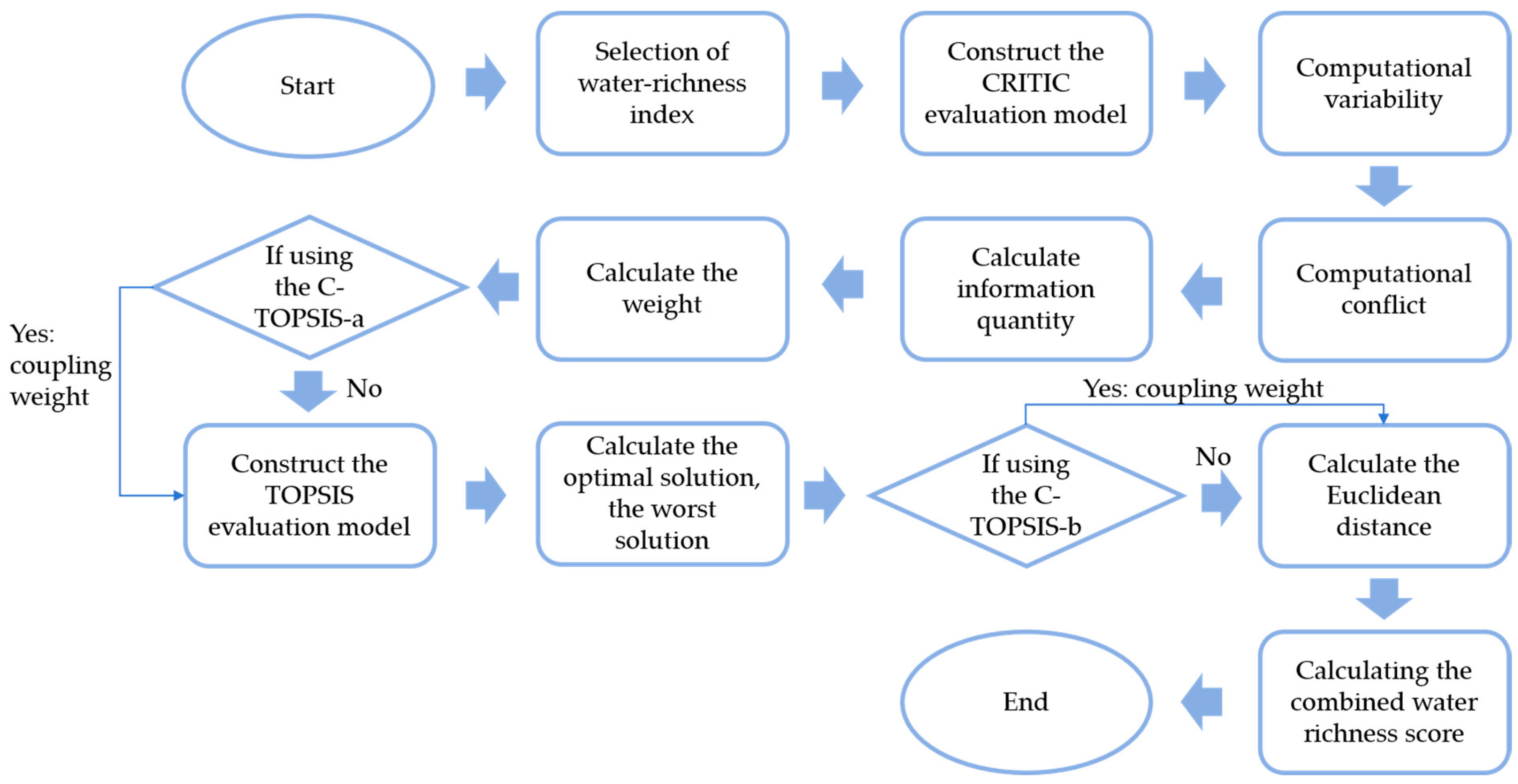
4. CRITIC-TOPSIS Model

4.1. CRITIC Objective Empowerment Method

The objective weighting method focuses on determining the weights of the evaluation indicators and assessing the subject of the evaluation based on the weights of the evaluation indicators [32]. The existing subjective assignment method chiefly relies on human interpretation, and the weight values vary from person to person, making it difficult to form a unified opinion, which leads to the assignment results being insufficiently precise and insufficiently credible. In the objective assignment method, the entropy value method and the coefficient of variation method utilize the magnitude of the difference of each indicator to obtain objective weights, but there is usually not only a difference but also a correlation between each evaluation indicator.

The CRITIC evaluation method reflects the amount of information contained in the data, which is obtained by solving for the variability and conflict within the indicators, resulting in the attainment of objective weights for the evaluation indicators. Variability draws on the idea of the standard deviation to represent the variability among the evaluation indicators. The larger the standard deviation value is, the more information the indicator contains. Conflict represents the correlations of the different indicators. The greater the correlation coefficient is, the stronger the correlation between the indicators is, and the lower the conflict is. CRITIC synthesizes the correlation and information weights between the water richness evaluation indicators contained in each borehole data, and the calculation results are objective and superior.

Regarding the calculation principle of the CRITIC evaluation method, using borehole data to construct the original evaluation matrix, dimensionless processing is performed to calculate the Pearson correlation coefficient, conflict, variability, and information quantity. The objective weights of each water richness evaluation index are then calculated.

4.2. TOPSIS Integrated Evaluation Method

The TOPSIS method measures the distance to the ideal solution, providing a comprehensive evaluation approach for multi-objective decision-making with limited alternatives. By integrating multiple attributes into a single attribute, it effectively reflects the overall situation, giving it the advantages of authenticity and intuitiveness. After applying consistent trend adjustment and normalization to the raw data, the influences of the different indicator units are eliminated. Additionally, by incorporating the original information from the data, the differences between the various schemes and the actual situation are objectively reflected. The finite number of evaluation objects is ranked according to their proximity to the idealized target, and the ideal optimal and worst solutions among the finite number of scenarios in the raw matrix of the normalized data are identified. Then, the distances between the evaluation program and the optimal program and the worst program are calculated separately to obtain the degree of proximity between the worst program and the best program. This is used as the basis for assessing the strengths and weaknesses of each evaluated object.

In the calculation principle of the TOPSIS evaluation method, the evaluation matrix U of the borehole data is constructed after the same trend and normalization process are applied, and the positive and negative ideal solutions—i.e., the maximum value and the minimum value of the evaluation indexes of the water enrichment of each borehole—are calculated. Next, the Euclidean distance of each borehole data point from the positive ideal solution or the negative ideal solution is calculated and combined with the Euclidean distance to produce a composite water richness score value.

4.3. CRITIC-TOPSIS Evaluation Methodology

The CRITIC and TOPSIS methods are combined in two ways, namely, C-TOPSIS-a and C-TOPSIS-b. The specific computational flow (Figure 6) and computational steps are described below.

Assume that there are m sets of borehole data to be evaluated and n water richness evaluation indicators.

1. To eliminate the impacts of the evaluation indicators, and take into account the original information of the data for each indicator, the data need to be normalized, calculated using Equations (5) and (6), and normalized so that all of the values are between 0 and 1, the direction of the impact is the same direction, and the processed matrix is E.

$$e_{ij}={\displaystyle \frac{x_{ij}-x_{\min j}}{x_{\max j}-x_{\min j}}}$$

(3)

$$e_{ij}={\displaystyle \frac{x_{\max j}-x_{ij}}{x_{\max j}-x_{\min j}}}$$

(4)

$$E=\left(\begin{array}{cccc}{e}_{11}& e_{12}& \dots & e_{1n}\\ e_{21}& e_{22}& \dots & e_{2n}\\ ⋮& ⋮& \ddots & ⋮\\ e_{m1}& e_{m2}& \dots & e_{mn}\end{array}\right)$$

(5)

In Equations (3)–(5), ${\mathit{e}}_{\mathit{i}\mathit{j}}$ is the normalized value of the jth evaluation indicator for the ith borehole, ${\mathit{x}}_{\mathit{i}\mathit{j}}$ is the original data for the jth evaluation indicator for the ith borehole, ${\mathit{x}}_{\mathit{m}\mathit{a}\mathit{x}\mathit{j}}$ is the maximum value of the borehole data for jth evaluation indicator, ${\mathit{x}}_{\mathit{m}\mathit{i}\mathit{n}\mathit{j}}$ is the minimum value of borehole data for the jth evaluation indicator, and E is the normalized data matrix.

The thickness of the sandstone aquifer, the ratio of the brittle–plastic rock thickness, and the fault fractal dimension are positive indicators and are processed using Equation (3). The core recovery rate and the number of sandstone–mudstone interbeds are negative indicators and are processed using Equation (4). Single-factor normalized thematic maps are then generated (Figure 7).

2. The variability of each evaluation indicator is determined. This is quantified through the standard deviation (Equation (6)):

$$S_j=\sqrt{{\displaystyle \frac{{\displaystyle \sum _{i=1}^m(e_{ij}-{\overline{e}}_j)}}{m-1}}}$$

(6)

where ${\mathit{S}}_{\mathit{j}}$ is the variability of the jth evaluation indicator, and $\overline{{\mathit{e}}_{\mathit{j}}}$ is the mean value of the normalized borehole data for the jth evaluation indicator.

3. The correlation coefficients between the evaluation indicators are calculated. The correlation coefficient serves as a statistical measure of the degree of association between the variables. Computed using the product-moment method, this coefficient quantifies the inter-variable relationships through multiplication of the deviations from their respective means (Equation (7)).

$$r_{jj+1}={\displaystyle \frac{{\displaystyle \sum _{i=1}^{\mathrm{m}}(e_{ij}-\overline{e_j})(e_{ij+1}-\overline{e_{j+1}})}}{\sqrt{{\displaystyle \sum _{i=1}^m{(e_{ij}-\overline{e_j})}^2{\displaystyle \sum _{i=1}^n{(e_{ij+1}-\overline{e_{j+1}})}^2}}}}}$$

(7)

where ${\mathbf{r}}_{\mathit{j}\mathit{j}+\mathbf{1}}$ is the correlation coefficient between the jth and (j + 1)th indicators, $\overline{{\mathit{e}}_{\mathit{j}}}$ is the mean value of the normalized borehole data for the jth indicator, $\overline{{\mathit{e}}_{\mathit{j}+\mathbf{1}}}$ is the mean value of the normalized borehole data for the (j + 1)th indicator, ${\mathit{e}}_{\mathit{i}\mathit{j}}$ is the normalized borehole data for the jth indicator for the ith sample, and ${\mathit{e}}_{\mathit{i}\mathit{j}+\mathbf{1}}$ is the normalized borehole data for the (j + 1)th indicator for the ith sample.

4. The conflict degree of each evaluation indicator is calculated as follows:

$$R_j={\displaystyle \sum _{j=1}^n(1-r_{jj+1})}$$

(8)

where ${\mathit{R}}_{\mathit{j}}$ is the conflict degree of the jth evaluation indicator.

5. The quantity of information of each indicator is determined. A larger quantity of information signifies greater importance of the corresponding indicator (Equation (9)):

$$F_j=S_j{\displaystyle \sum _{j=1}^n(1-r_{jj+1})=S_j{R}_j}$$

(9)

where ${\mathit{F}}_{\mathit{j}}$ is the quantity of information of the jth evaluation indicator.

6. The weight for each water abundance evaluation indicator is calculated as follows:

$$w_j={\displaystyle \frac{F_j}{{\displaystyle \sum _{\mathrm{j}=1}^n{F}_j}}}$$

(10)

where ${\mathit{W}}_{\mathit{j}}$ is the weight of the jth evaluation indicator.

7. The data are subjected to squared summation normalization, yielding the normalized matrix (Equation (11)):

$$U={\displaystyle \frac{e_{ij}}{\sqrt{{\displaystyle \sum _{i=1}^m{e}_{ij}^2}}}}=\left(\begin{array}{cccc}{u}_{11}& u_{12}& \dots & u_{1n}\\ u_{21}& u_{22}& \dots & u_{2n}\\ ⋮& ⋮& \ddots & ⋮\\ u_{m1}& u_{m2}& \dots & u_{mn}\end{array}\right)$$

(11)

where $\mathbf{U}$ is the normalized data matrix.

8. In this stage, the C-TOPSIS-a method integrates the CRITIC method weights with matrix U, generating the weighted standardized matrix (Equation (12)):

$$u=w_j\times \left(\begin{array}{cccc}{u}_{11}& u_{12}& \dots & u_{1n}\\ u_{21}& u_{22}& \dots & u_{2n}\\ ⋮& ⋮& \ddots & ⋮\\ u_{m1}& u_{m1}& \dots & u_{mn}\end{array}\right)=\left(\begin{array}{cccc}{w}_1{u}_{11}& w_2{u}_{12}& \dots & w_n{u}_{1n}\\ w_1{u}_{21}& w_2{u}_{22}& \dots & w_n{u}_{2n}\\ ⋮& ⋮& \ddots & ⋮\\ w_1{u}_{m1}& w_2{u}_{m2}& \dots & w_n{u}_{mn}\end{array}\right)$$

(12)

where u is the weighted data matrix.

9. The optimal and worst solutions are determined for each evaluation indicator (Equations (13) and (14)):

$$u_j^{+}=\underset{mj}{\max }(u_1^{+},u_2^{+},\dots ,u_n^{+})$$

(13)

$$u_j^{-}=\underset{mj}{\min }(u_1^{-},u_2^{-},\dots ,u_n^{-})$$

(14)

where ${\mathit{u}}_{\mathit{j}}^{+}$ is the optimal solution for the jth indicator, and ${\mathit{u}}_{\mathit{j}}^{-}$ is the worst solution for the jth indicator.

10. The Euclidean distance between each borehole dataset and either the optimal solution or the negative ideal solution is calculated (Equations (15) and (16)):

$$I_i^{+}=\sqrt{{\displaystyle \sum _{j=1}^n{(u_{ij}-u_j^{+})}^2}}$$

(15)

$$I_i^{-}=\sqrt{{\displaystyle \sum _{j=1}^n{(u_{ij}-u_j^{-})}^2}}$$

(16)

where ${\mathit{I}}_{\mathit{i}}^{+}$ is the Euclidean distance between the ith borehole dataset and the optimal solution, and ${\mathit{I}}_{\mathit{i}}^{-}$ is the distance between the ith borehole dataset and the worst solution.

In this stage, the C-TOPSIS-b method introduces the weights derived using the CRITIC method into the TOPSIS Euclidean distance calculation (Equations (17) and (18)):

$$I_i^{+}=\sqrt{{\displaystyle \sum _{j=1}^n{w}_j{(u_{ij}-u_j^{+})}^2}}$$

(17)

$$I_i^{-}=\sqrt{{\displaystyle \sum _{j=1}^n{w}_j{(u_{ij}-u_j^{-})}^2}}$$

(18)

11. The water abundance composite score is calculated by integrating the Euclidean distances. A higher score indicates stronger water abundance characteristics (Equation (19)):

$$C_i={\displaystyle \frac{I_i^{-}}{I_i^{+}+I_i^{-}}}$$

(19)

where ${\mathit{C}}_{\mathit{i}}$ is the water abundance composite score for the ith borehole.

5. Discussion of the Results

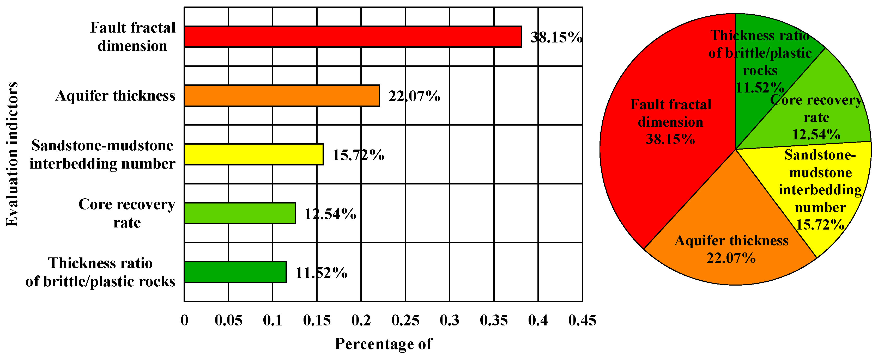
5.1. Weighting Analysis of Main Controlling Factors

The CRITIC method was utilized to solve for the weight values affecting the water richness of the sandstone above the main mining coal seam (Figure 8). The weight values influencing the water richness of the sandstone in the roof strata of the main coal seam, calculated using the CRITIC method, are shown in Figure 8. As indicated by the water richness indicator weighting diagram, the fault fractal dimension (38.15%) and aquifer thickness (22.07%) have the highest weights and thus exert pronounced influences on the water richness of the roof sandstone. The sandstone–mudstone interbeds (15.72%) have a moderate weight, and the core recovery (12.54%) and brittle–plastic rock thickness ratio (11.52%) have smaller weights. The latter three water richness evaluation indexes have relatively little effect on the water richness of the top sandstone.

As discussed earlier, the development of faults has indirectly influenced the aquifers. The CRITIC evaluation method assigned weights of 38.15% to the fault fractal dimension and 22.07% to the aquifer thickness, and their combined weights account for 60.22% of the total. The fault development cuts aquifers and disrupts the integrity of the stratigraphic rock mass, leading to the conclusion that the water richness of the coal seam’s roof sandstone has been strongly influenced by the fault activity and aquifer thickness. The brittle–plastic rock thickness ratio, with a weight of 11.52%, exerts the least influence on the water richness of the roof. This is primarily because the variations in the brittle–plastic rock thickness are concentrated in the southwestern corner of the mining field, resulting in limited impact in the other regions.

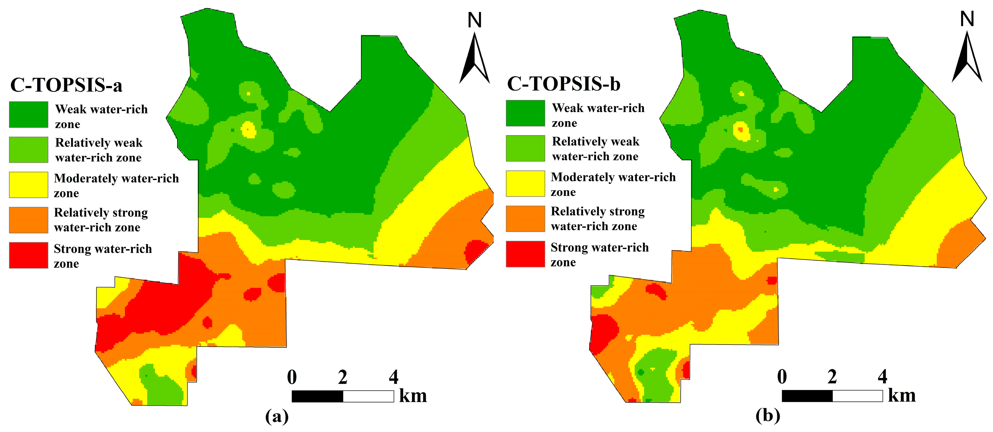
5.2. Comparison of Water Richness Evaluation Results

The water richness indicators were calculated using the C-TOPSIS-a and C-TOPSIS-b evaluation methods. The water abundance scores (C_i) were classified into five categories using the natural breaks classification method: weak water richness zone, relatively weak water abundance zone, moderate water abundance zone, relatively strong water abundance zone, and strong water abundance zone (Figure 9). The water richness of the roof sandstone in the main mining coal seam exhibits a general trend of stronger water richness in the southwestern part and weaker water richness in the northern region. The C-TOPSIS-a evaluation method involves superimposition of the indicator weights during the transition phase with the TOPSIS evaluation method, while the C-TOPSIS-b evaluation method directly incorporates the weights of the indicator factors into the internal TOPSIS framework, in which they participate in the Euclidean distance calculation. While the two methods exhibit certain discrepancies in their calculation results, they exhibit a high degree of similarity in the water richness zoning classification approach.

To intuitively compare the water richness zoning results of the two evaluation methods, the Pearson correlation coefficients between the C-TOPSIS-a and C-TOPSIS-b evaluation methods and the CRITIC and TOPSIS evaluation methods were calculated. The results are presented in

Table 3. Pearson’s correlation coefficient.

Evaluation Methods	CRITIC	TOPSIS	C-TOPSIS-a	C-TOPSIS-b
CRITIC	1	0.681615876	0.95142371	0.872978244
TOPSIS	0.681615876	1	0.771228086	0.931244354
C-TOPSIS-a	0.95142371	0.771228086	1	0.949398919
C-TOPSIS-b	0.872978244	0.931244354	0.949398919	1

. The correlation between the C-TOPSIS-a evaluation method and the CRITIC evaluation method reaches 0.9514, demonstrating that the C-TOPSIS-a method is predominantly influenced by the indicator weights derived from the CRITIC method, while it is less influenced by the TOPSIS evaluation method. In contrast, the correlation coefficients between the C-TOPSIS-b evaluation method and the CRITIC and TOPSIS evaluation methods are 0.8730 and 0.9312, respectively. This demonstrates that the C-TOPSIS-b method integrates the characteristics of both the CRITIC and TOPSIS, accounting for the influence of the indicator weight constraints while also incorporating the distance to the positive and negative ideal solutions. Through comprehensive analysis, the superiority of the two methods was ranked as follows: C-TOPSIS-b > C-TOPSIS-a.

5.3. Validation of Evaluation Results

A total of 22 drainage boreholes were deployed in the tailgate and 2 gate roads of working face 103 in the main coal seam. All of the boreholes were drilled from the roof of the coal seam roadway. Their orientations are shown in Figure 10. Water discharge drill holes T1–T8 are located at the location of the working face cuttings. Due to the installation of synthesized mining equipment, the last measured gushing water data for the cuttings were compared. The cumulative total water influx from boreholes T1–T4 and T8, which were located in the area of moderate water richness, was 1628.37 m³; and the cumulative total water influx from boreholes T5–T7, which were located in the area of stronger water richness, was 1288.94 m³. The average borehole water influx in the more water-rich area at the workface cuttings was 103.97 m³ more than the average borehole water influx in the moderately water-rich area. In the Shun Trough, among drill holes T9–T11, T18, T20, and T22, which were located in the area of weaker water richness, the cumulative water influx was only 48.96 m³ in T20, drenching only occurred in T18, and water was not present in the rest of the drill holes. Borehole T21, located in the weak water-rich zone, did not exhibit water inflow. In borehole T16, situated in the strong water-rich zone, a cumulative water inflow of 2677.98 m³ was recorded. In boreholes T12–T14, T15, T17, and T19, located in the moderate water-rich zone, a cumulative water inflow of 15,804.98 m³ was recorded, with an average of 2634.16 m³ per borehole. The water inflow in the strong and moderate water-rich zones significantly exceeded that in the weak water-rich zone. The measured water inflow data validate the accuracy of the water richness zoning in the roof of the main mining coal seam.

Based on verification of the results of the water exploration and discharge drill holes in the working face, the method was effective in evaluating the sandstone in the Yanan Formation, and it is suitable for evaluating the water richness of aquifers under similar geological conditions. However, for areas with complex geological bodies and strong tectonic activity, it is necessary to improve the accuracy of the borehole survey and modify the model water richness evaluation indexes to ensure the applicability of the evaluation results.

6. Conclusions

(1) To evaluate the water richness of the sandstone aquifer in the Yanan Formation, five main control factors were considered. The CRITIC objective weighting method was used to solve for the weight of each main controlling factor. The weights of the aquifer thickness, brittle–plastic rock thickness ratio, core recovery rate, number of sandstone and mudstone interbeds, and fault subdimensional value were determined to be 22.07, 11.52, 12.54, 15.72, and 38.15%. The thicknesses of the faults and aquifers had large effects on the water richness.

(2) The evaluation results of the C-TOPSIS-a and C-TOPSIS-b have similar trends, but the correlation coefficients between the C-TOPSIS-a and the CRITIC and TOPSIS are 0.9514 and 0.7712, respectively. In addition, the C-TOPSIS-a evaluation method was greatly affected by the weights of the indicator factors of the CRITIC evaluation method. The results of the C-TOPSIS-b evaluation method are similar to the CRITIC evaluation method. The correlation coefficients between the C-TOPSIS-b and the CRITIC and TOPSIS are 0.8730 and 0.9312 respectively, so the C-TOPSIS-b evaluation method utilizes the advantages of both the CRITIC and TOPSIS evaluation methods. The advantages and disadvantages of the two methods are as follows: C-TOPSIS-b > C-TOPSIS-a.

(3) The C-TOPSIS-b evaluation method categorizes the water richness levels of the boreholes and generates a zoned water richness map based on the water richness index results. A five-category classification of the water richness in the study area was developed: weak, moderately weak, moderate, relatively strong, and strong. The weak and moderately weak zones predominantly occur in the northern sector, the moderate zones are concentrated in the central-southern sector, and the strong and relatively strong zones are primarily distributed in the southwestern sector. Overall, the sandstone aquifer exhibits water richness levels ranging from weak to relatively strong. Validation through measured water inflow data confirmed the rationality and accuracy of this methodology for sandstone aquifer zoning, demonstrating its applicability to water richness evaluation in areas with similar stratigraphic conditions.

References

1. Zeng, Y.; Zhu, H.; Wu, Q.; Guo, X.; Pang, Z.; Liu, S.; Yang, W. Research status and prevention and control path of coal seam roof water disaster in China. J. China Coal Soc. 2024, 50, 1073–1099. [Google Scholar]
2. Wang, C.; Zhao, Y.; Ning, L.; Bi, J. Permeability evolution of coal subjected to triaxial compression based on in-situ nuclear magnetic resonance. Int. J. Rock Mech. Min. Sci. 2022, 159, 105213. [Google Scholar] [CrossRef]
3. Dong, H.; Yang, G.; Guo, K.; Xu, J.; Liu, D.; Han, J.; Shi, D.; Pan, J. Predicting water flowing fracture zone height using GRA and optimized neural networks. Processes 2024, 12, 2513. [Google Scholar] [CrossRef]
4. Zhai, P.; Li, N. Predicting the height of the hydraulic fracture zone using a convolutional neural network. Mine Water Environ. 2023, 42, 500–512. [Google Scholar] [CrossRef]
5. Cheng, J.; Zhao, J.; Dong, Y.; Dong, Q. Quantitative prediction of water abundance in rock mass by transient electro–magnetic method with LBA—BP neural network. J. China Coal Soc. 2020, 45, 330–337. [Google Scholar]
6. Hou, E.; Wu, J.; Yang, F.; Zhang, C. Evaluation of Water-richness of Weathered Bedrock Based on the WOA-SVM Discriminant Model: Take Zhangjiamao Coal Mine in Shenfu Coal Field as an Example. Sci. Technol. Eng. 2025, 25, 119–127. [Google Scholar]
7. Hou, E.; Ji, Z.; Che, X.; Wang, J.; Guo, L.; Tian, S.; Yang, F. Water-richness prediction method for weathered bedrock based on the coupling of improved AHP and entropy weight method. J. Coal 2019, 44, 3164–3173. [Google Scholar]
8. Hou, E.; Li, Q.; Yang, L.; Bi, M.; Li, Y.; He, Y. Prediction of Water-Richness Zoning of Weathered Bedrock Based on Whale Optimisation Algorithm and Random Forest. Water 2025, 16, 3655. [Google Scholar] [CrossRef]
9. Jiang, W. Study on the Prediction of Sudden Water Hazard in Hanglaiwan Coal Mine in Yushen Mining Area. Master’s Thesis, China University of Mining and Technology, Beijing, China, 2022. [Google Scholar]
10. Niu, C.; Tian, Q.; Xiao, L.; Xue, X.; Zhang, R.; Xu, D.; Luo, S. Principal causes of water damage in mining roofs under giant thick topsoil-lilou coal mine. Appl. Water Sci. 2024, 14, 146. [Google Scholar] [CrossRef]
11. Xiao, L.; Li, F.; Niu, C.; Dai, G.; Qiao, Q.; Lin, C. Evaluation of water inrush hazard in coal seam roof based on the AHP-CRITIC composite weighted method. Energies 2022, 16, 114. [Google Scholar] [CrossRef]
12. Fang, G. Water-rich zoning and water quantity prediction of coal seam in Balasu Mine Field. Saf. Coal Mines 2024, 55, 200–207. [Google Scholar]
13. Lyu, Z.; Meng, F.; Lyu, W.; Li, L. Improved Method for Predicting and Evaluating Water Yield Property. Coal Technol. 2023, 42, 152–155. [Google Scholar]
14. Sun, K.; Miao, Y.; Chen, X.; Wang, H.; Fan, L.; Yang, L.; Ma, W.; Lu, B.; Li, C.; Chen, J.; et al. Occurrence characteristics and water abundance of Zhiluo Formation in nortnern Ordos Basin. J. China Coal Soc. 2022, 47, 3572–3598. [Google Scholar]
15. Kuo, W.; Li, X.; Zhang, Y.; Li, W.; Wang, Q.; Li, L. Prediction Model of Water Abundance of Weakly Cemented Sandstone Aquifer Based on Principal Component Analysis–Back Propagation Neural Network of Grey Correlation Analysis Decision Making. Water 2024, 16, 551. [Google Scholar] [CrossRef]
16. Chen, X.; Li, S.; Bian, K.; Yang, H.; Chang, J. Risk assessment of water inrush based on FAHP-EWM combined weighting method. Coal Mine Saf. 2024, 55, 184–193. [Google Scholar]
17. Yang, L.; Bao, K.; Hou, E.; Lu, B.; Li, Y. Evaluation of water richness of weathered bedrock aquifers based on subjective and objective combination of TOPSIS-RSR. Coal Sci. Technol. 2024. [Google Scholar]
18. Bai, Y.; Niu, C.; Li, F.; Xiang, M.; Zhao, S. Water abundance evaluation of weathered bedrock aquifers based on FAHP and coefficient of variance method. Saf. Coal Mines 2023, 54, 143–149. [Google Scholar]
19. Liang, G.; Wan, B.; Feng, L.; Zhang, R.; Jiao, J.; Hou, L.; Li, Y.; Gu, L. Water-richness evaluation of Luohe Formation aquifer above coal seam based on combination weighting method. Coal Sci. Technol. 2024, 52, 201–210. [Google Scholar]
20. Zhao, Y.; Bi, J.; Wang, C.; Liu, P. Effect of unloading rate on the mechanical behavior and fracture Characteristics of Sandstones under complex triaxial stress conditions. Rock Mech. Rock Eng. 2021, 54, 4851–4866. [Google Scholar] [CrossRef]
21. Zhao, Y.; Liu, H. An elastic Stress-Strain relationship for porous rock under anisotropic stress conditions. Rock Mech. Rock Eng. 2012, 45, 389–399. [Google Scholar] [CrossRef]
22. Zhao, Y.; Wang, C.; Bi, J. Analysis of fractured rock permeability evolution under unloading conditions by the model of elastoplastic contact between rough surfaces. Rock Mech. Rock Eng. 2020, 53, 5795–5808. [Google Scholar] [CrossRef]
23. Du, H.; Liu, Y.; Bi, Y.; Sun, H.; Ning, B. Spatial-temporal heterogeneity of landscape ecological risk in Yushenfu Mining Area from 1995 to 2021. Coal Sci. Technol. 2024, 52, 270–279. [Google Scholar]
24. Liu, J.; Zhu, G.; Liu, Y.; Chao, W.; Du, J.; Yang, Q.; Mi, H.; Zhang, S. Breakthrough, future challenges and countermeasures of deep coalbed methane in the eastern margin of Ordos Basin: A case study of Linxing-Shenfu block. Acta Pet. Sin. 2023, 44, 1827–1839. [Google Scholar]
25. Wang, Y.; Pu, Z.; Ge, Q.; Liu, J. Study on the water-richness law and zoning assessment of mine water-bearing aquifers based on sedimentary characteristics. Sci. Rep. 2022, 12, 14107. [Google Scholar] [CrossRef] [PubMed]
26. Qiu, M.; Shao, Z.; Zhang, W.; Zheng, Y.; Yin, X.; Gai, G.; Han, Z.; Zhao, J. Water-richness evaluation method and application of clastic rock aquifer in mining seam roof. Sci. Rep. 2024, 14, 6465. [Google Scholar] [CrossRef] [PubMed]
27. Xu, J.; Wang, Q.; Zhang, Y.; Li, W.; Li, X. Evaluation of coal-seam roof-water richness based on improved weight method: A case study in the dananhu No. 7 coal mine, China. Water 2024, 16, 1847. [Google Scholar] [CrossRef]
28. Gai, G.; Qiu, M.; Zhang, W.; Shi, L. Evaluation of water richness in coal seam roof aquifer based on factor optimization and random forest method. Sci. Rep. 2024, 14, 24421. [Google Scholar] [CrossRef]
29. Liu, X.; Li, P.; Xu, J. Fractal dimension calculation of fault system and discussion on its relation to the deep-source gas migration. Nat. Gas Ind. 1998, 18, 27–30+23–24. [Google Scholar]
30. Zhao, J.; Li, J.; Zhang, Z.; Yang, C.C.; Zhang, X.J. Multifractal characteristics of spatial distribution of the faults in west subsag of Bozhong Sag. Oil Drill. Prod. Technol. 2018, 40, 14–16. [Google Scholar]
31. Li, F.; Liu, G.; Zhou, Q.; Zhao, G. Application of fractal theory in the study of the relationship between fracture and mineral. J. Hefei Univ. Technol. 2016, 39, 701–706. [Google Scholar]
32. Lyu, Z.; Wu, M.; Song, Z.; Zhao, T.; Du, G. Comprehensive evaluation of power quality on CRITIC-TOPSIS method. Electr. Mach. Control 2020, 24, 137–144. [Google Scholar]
Figure 1. Schematic location of the study area.
Water 17 01424 g001
Figure 2. Stratigraphic cross-sections and stratigraphic column for the study area.
Water 17 01424 g002
Figure 3. Contour plots of the main controlling factors. (a) is a contour map of the aquifer thickness; (b) is a contour map of the thickness ratio of brittle/plastic rocks; (c) is a contour map of the core recovery rate; (d) is a contour map of the sandstone-mudstone interbedding number; (e) is a contour map of the fault fractal dimension.
Water 17 01424 g003
Figure 4. Grid cell partitioning.
Water 17 01424 g004
Figure 5. lgN(r) versus lgr regression curve.
Water 17 01424 g005
Figure 6. Comprehensive water richness evaluation process.
Water 17 01424 g006
Figure 7. One-factor normalized thematic map. (a) is a thematic map of aquifer thickness normalization; (b) is a thematic map of thickness ratio of brittle/plastic rocks normalization; (c) is a (b) is a thematic map of core recovery rate normalization; (d) is a thematic map of sandstone-mudstone interbedding number normalization; (e) is a thematic map of fault fratal dimension normalization.
Water 17 01424 g007
Figure 8. Weighting of water enrichment indicators.
Water 17 01424 g008
Figure 9. Water richness zoning. (a) is the C-TOPSIS-a water-richness zoning map; (b) is the C-TOPSIS-b water-richness zoning map.
Water 17 01424 g009
Figure 10. Design of exploratory boreholes.
Water 17 01424 g010