A Network-Based Clustering Method to Ensure Homogeneity in Regional Frequency Analysis of Extreme Rainfall

Abstract

The social impacts of extreme rainfall events are expected to intensify with climate change, making reliable statistical analyses essential. High quantile estimation requires substantial data; however, available records are sometimes limited. Additionally, finite data and variability across statistical models introduce uncertainties in the final estimates. This study addresses the uncertainty that arises when selecting parameters in Regional Frequency Analysis (RFA) by proposing a method to objectively identify statistically homogeneous regions. Station coordinates, elevation, annual mean rainfall, maximum annual rainfall, and l-skewness from 55 meteorological stations are selected to study annual maximum daily rainfall. These covariates are employed to investigate the interdependency of the covariates in Principal Component Analysis (PCA) as a preprocessing step in cluster analysis. Network theory, implemented through an iterative clustering process, is used in network creation where stations are linked based on the frequency of their co-occurrence in clusters. Communities are formed by maximizing the modularity index after creating a network of stations. RFA is performed in the final communities using L-moment theory to estimate regional and InSite quantiles. Quantile uncertainty is calculated through parametric bootstrapping. The application of PCA has a negligible effect on network creation in the study area. The results show that the iterative clustering approach with network theory ensures statistically created homogeneous regions, as demonstrated in Thessaly’s complex terrain for regionalisation of extreme rainfall.

1. Introduction

Climate change is expected to amplify the already big societal consequences that extreme rainfall events have [1]. Because the infrastructure in urban environments, especially the water systems, is vulnerable, it is necessary to reliably statistically analyse these events [2]. For high quantile estimation, a large amount of data is required but there is not a specific agreed-upon record length. In many cases, because of negligence or even the absence of rainfall stations historical records are scarce or unavailable [3]. Therefore the development of a method to transfer and group information is of extreme importance [4]. The grouped statistical analysis is called regional frequency analysis and in the literature, many different methods have been proposed [5]. An important variant of RFA is the “index flood” method [6,7]. This method is based on the assumption that if we split the study area into statistically homogenous regions, and the data inside the defined regions are scaled by an index statistic (e.g., median, mean value) can be described by a common parent distribution [8].

Hosking and Wallis [9] proposed a unified approach, merging the index-flood technique with the L-moments, estimating quantiles and regional parameters as well as constructing regional statistics, and creating homogenous areas. This method has been used for regional analysis of many different variables such as such as floods [10,11,12], droughts [13,14,15] and extreme rainfall [16,17,18,19,20,21,22,23] and is considered to be among the most relevant and efficient approaches [24].

The process, proposed by Hosking and Wallis [9], has the following steps. First, data are pre-processed to address errors and inconsistencies. Homogeneous regions are then identified to ensure that data within each region follow identical distributions. Appropriate probability distributions are fitted to the pooled and scaled data for each homogeneous region using L-moments. Finally, desired quantiles are calculated with the “index-flood” method. Regional homogeneity in RFA is assessed using the heterogeneity measure $H_n$. This criterion evaluates the sample L-moment ratios of the region against those expected in a homogeneous region. A region with $H_n\ge 2$ is considered “definitely heterogenous” [9]. Despite various approaches for identifying homogeneous regions, there is no guarantee that the resulting regions will have $H_n<2$.

There is no single, universally accepted method for performing frequency analysis of extreme precipitation events. Even within the framework established by Hosking and Wallis, various procedural variants have been proposed. Treating Regional Frequency Analysis (RFA) as a statistical model, different types of uncertainties can impact the accurate estimation of high quantiles [25]. Key sources of uncertainty include data characteristics (such as correlation, stationarity, and record length), choice of frequency distribution, parameter estimation, and the homogeneity of the regions where data pooling occurs [26]. Creating statistically homogeneous regions often requires station covariates. In the international bibliography, different covariates are used, including elevation, average annual maximum rainfall depth, and mean annual dry days. Dinpashoh et al. [27] used 57 covariate (mainly climatological) variables in a principal component analysis of 77 weather stations. Feidas et al. [28] studied precipitation and air temperature patterns in Greece. Using Pearson’s correlation coefficient, they identified factors (i.e., NDVI-Normalized Difference Vegetation Index, spatial coordinates and elevation) that most affect the spatial variability of these weather patterns. Additionally, elevation has shown that is a suitable explanatory variable in the design of intensity-duration-frequency curves in Thessaly region [29]. In the same region, several studies show the importance of spatial covariates and elevation in monthly rainfall analysis [30,31]. In the Mediterranean, the same covariates are identified for extreme rainfall [23,32]. Finally, Hosking & Wallis [9], recommend using location, elevation, and rainfall to form homogeneous regions in RFA.

A critical step in regional frequency analysis is defining homogeneous regions. Commonly, study areas are delineated based on climate, geographical, or topographical boundaries, however, this approach may not guarantee statistical homogeneity, as rainfall characteristics can vary significantly within continuous areas. To improve homogeneity, alternative methods are employed, including cluster analysis (CA), self-organizing maps (SOM), regions of interest (ROI), principal component analysis (PCA), or PCA combined with CA [5,27,33,34,35,36,37,38,39,40,41,42]. Multivariate cluster analyses have also been used to analyse the non-stationarity of extreme precipitation with teleconnection indices [43,44]. Recent studies in hydrology utilize complex networks and community detection, originally derived from social network analysis, to group hydrological variables [45,46,47,48,49,50]. This method involves two main steps: creating a network by determining links between stations using a similarity metric and applying a community detection algorithm to group similar stations [51]. Correlation [52] and mutual information (MI) [53] are commonly used as similarity metrics in the first step. For the second step, the crucial factor is the setting of a threshold for the similarity metric that determines which nodes are connected in the network. Various methods exist, including selecting thresholds based on network metrics like modularity [54,55], but further research is needed to develop a standardized approach [50].

Multivariate analysis and clustering techniques with applications in RFA show inconsistencies in identifying homogenous regions. Forestieri et al. [1] used PCA and the k-means algorithm to identify homogeneous groups in Sicily, Italy, with annual maximum precipitation data. They found potential heterogeneity in the North-Center region (1-h duration) and the Center-South region (6-h and 12-h durations). Gall et al. [20] using daily precipitation data in Switzerland, compared traditional RFA with their modified clustering algorithm and found that all regions showed strong heterogeneity, especially in the Alpine areas. Finally, Joo et al. [49] showed the potential of using network theory in delineating homogenous regions for flood frequency analysis when compared with multivariate clustering techniques.

Studies on defining homogeneous regions typically follow a “top-down” approach, where all stations in the study area are grouped into regions, which are then assessed for homogeneity; heterogenous regions undergo further adjustments, including station exclusion. Our methodology, by contrast, adopts a “bottom-up” approach to minimize the subjectivity of covariate selection. For this implementation, we use PCA and Non-PCA cluster analysis to study annual daily maximum rainfall in the Thessaly region. Several station covariates are selected based on preliminary RFA in the Thessaly area [56]. Station coordinates, elevation, annual mean rainfall, maximum annual rainfall, and l-skewness are proven reliable covariates in studying annual maximum extreme rainfall. These covariates are employed in this study to investigate the interdependency of the covariates in PCA as a preprocessing step in cluster analysis. Through an iterative clustering process using all possible covariate combinations, we create a network where stations are linked based on the frequency of their co-occurrence in clusters at the end of the process. Final communities are formed by maximizing the modularity index in the station network and in these communities; RFA is performed using L-moments theory.

2. Materials and Methods

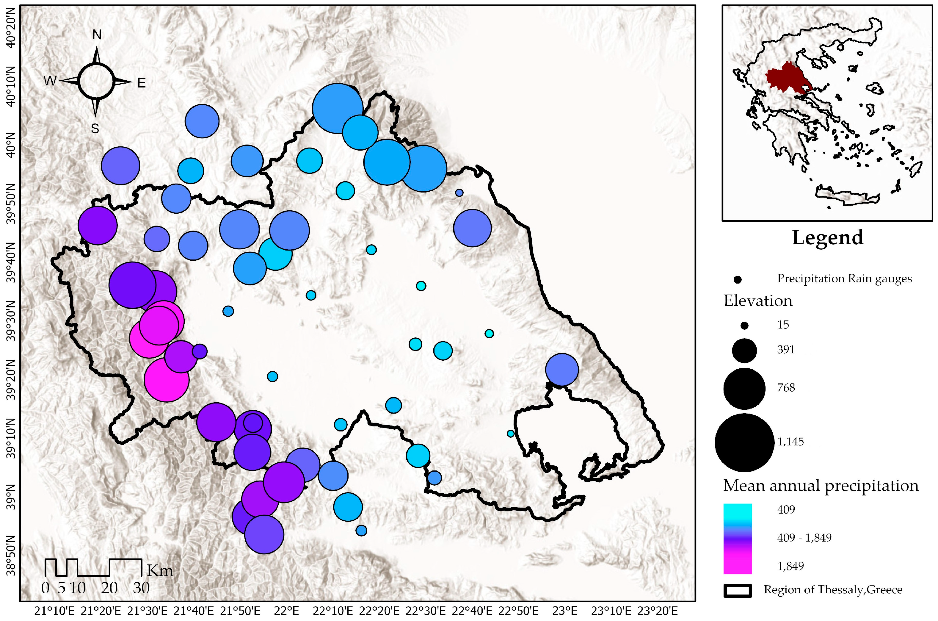
2.1. Study Area and Data Sources

Thessaly (Figure 1) is located in central Greece and covers a total area of about 14,000 km², 11% of the total area of the country with an average altitude of 500 m is bordered by Pelion and the Aegean Sea to the east, Mount Olympus to the north, Pindos to the west, and Mount Othrys to the south. The central Thessalian plain, traversed by the Pinios River and its tributaries, lies within these mountainous boundaries. In terms of climate, Thessaly has hot, dry summers with temperatures reaching 40 °C in July and August. Average annual rainfall in Thessaly ranges from 400 mm at low altitudes to 1850 mm in the western mountain range. The average precipitation is 700 mm [57]. The variations in the spatial characteristics of the region make Thessaly a valuable region for the analysis of extreme precipitation and how it depends on various geographical variables.

For the analysis of extreme precipitation, we use the rainfall database developed in a recent study [29] for the region of Thessaly. In this study, comprehensive quality control procedures are applied to ensure the reliability and accuracy of the rainfall data. Further details can be found in Iliopoulou et al. [29]. Most rainfall stations are in the western part of the Pindos mountain range, from north to south, because this area receives the highest rainfall. However, as we move east, the number of rain gauges decreases significantly (Figure 1). The data used are annual 24-h rainfall maxima from 55 precipitation stations.

Table 1. Summary statistics for the rain gauges in the region of Thessaly.

	Min	${\mathit{Q}}_{25}$	${\mathit{Q}}_{50}$	${\mathit{Q}}_{75}$	Max
Elevation (m)	15	282	688	850	1179
Number of data (years)	15	31	44	62	69

presents summary statistics for the rain gauges in Thessaly, showing the minimum, 25th percentile, median, 75th percentile, and maximum values for elevation and the number of years of data available. The station at the lowest altitude is in Anchialos, at 15 m, while the highest station is in Livadi, at 1179 m. The station with the shortest operating time is Pythio (15 years), and the longest-operating station is Meteora (69 years). The intermediate time of operation is 44 years, ranging from 1940 to 2013.

Table A1. Station characteristics.

Name	X	Y	Z	Mean Annual Precipitation	Mean of Maximun Annual Daily Rainfall	Lca
Agchialos	396,203.00	4,341,105.00	15.00	501.72	55.31	0.24
Agiofyllo	291,669.00	4,415,392.00	600.00	790.78	59.40	0.15
Agrelia	322,649.00	4,397,952.00	700.00	548.35	48.60	0.14
Amarantos	315,620.00	4,342,587.00	800.00	1159.08	86.97	−0.02
Anavra	372,326.70	4,327,101.00	208.00	735.11	73.81	0.21
Argithea	288,679.00	4,358,079.00	992.00	1649.70	80.02	0.12
Chrysomilia	285,140.00	4,385,948.00	940.00	1238.19	95.38	0.02
Drakotrypa	293,185.00	4,365,363.00	680.00	1336.82	81.95	0.24
Elassona	344,494.00	4,417,838.00	314.00	538.81	59.04	0.41
ElatiDEH	313,872.20	4,427,213.00	663.60	734.38	65.96	0.14
ElatiYPEKA	287,748.00	4,376,618.00	900.00	1630.37	99.38	0.24
Farkadona	333,800.00	4,384,747.00	87.00	548.58	55.74	0.24
Farsala	359,598.90	4,350,003.00	250.00	627.10	62.56	0.19
FragmaPlastira	304,154.00	4,344,717.00	850.00	1241.14	84.85	0.00
Giannota	333,296.00	4,427,329.00	500.00	583.38	57.70	0.20
Kallipeyki	368,844.00	4,424,784.00	1050.00	710.89	97.11	0.45
Karditsa	321,757.00	4,359,103.00	103.00	607.73	62.90	0.36
Karpero	296,204.00	4,424,125.00	504.40	638.67	45.50	0.25
Kipourgio	274,279.30	4,425,745.00	828.20	916.37	49.46	0.07
Koniskos	311,401.00	4,405,624.00	860.00	800.00	62.84	0.23
Kryovrisi	357,491.00	4,426,838.00	1030.00	679.91	59.75	0.33
Larisa	368,210.00	4,387,785.00	79.00	414.67	48.11	0.38
Liopraso	314,719.40	4,393,282.00	688.00	713.12	60.87	0.03
LivadiYPEKA	342,182.00	4,443,797.00	1179.00	718.00	64.14	0.17
LivadiYPGE	342,182.00	4,443,797.00	1179.00	718.49	62.70	0.29
Loutsopigh	331,211.00	4,331,131.00	730.00	916.89	72.95	0.28
Magoyla	343,054.60	4,343,956.00	170.00	581.52	51.10	0.14
Makrinitsa	412,260.00	4,361,258.00	690.00	836.88	103.59	0.16
Makryraxh	340,690.60	4,327,788.00	602.90	777.98	60.35	0.18
Malakasio	267,150.00	4,406,840.00	842.00	1209.57	67.39	0.08
Megalh_kerasia	285,604.00	4,402,599.00	500.00	889.16	67.71	0.10
Meteora	296,980.00	4,400,438.00	596.00	809.63	69.17	0.19
Moloha	315,446.00	4,335,188.00	790.00	1092.66	89.76	0.13
Moyzaki	298,972.00	4,367,063.00	226.00	1128.61	64.78	−0.07
Myra	375,034.00	4,367,317.00	320.00	535.48	55.65	0.19
Neoxori	314,969.00	4,314,839.00	800.00	1100.05	80.68	0.13
Paleioxori	278,037.00	4,388,000.00	1050.00	1166.62	88.84	0.14
Pitsiota	317,985.00	4,320,322.00	800.00	1287.63	61.45	0.30
Pyloroi	299,745.90	4,439,832.00	715.10	793.03	40.12	0.13
Pyrgetos	380,116.00	4,417,196.00	31.00	797.63	81.07	0.04
Pythio	349,135.00	4,436,253.00	750.00	648.67	60.42	0.39
Raxhoyla	315,664.00	4,344,437.00	330.00	1122.11	72.34	−0.09
Redina	325,324.00	4,325,708.00	903.00	1253.70	66.23	0.31
Skopia	367,299.00	4,334,140.00	450.00	547.24	57.29	0.27
Sphlia	384,223.00	4,406,031.00	813.00	848.79	103.41	0.20
Stoyrnaraiika	283,294.00	4,371,187.00	860.00	1849.46	113.00	0.18
Swthrio	389,455.00	4,372,649.00	54.00	409.02	63.07	0.36
Trikala	307,901.00	4,379,795.00	114.00	697.73	54.79	0.04
Trilofo	345,367.00	4,317,887.00	580.00	632.52	52.54	0.08
Tymfristos	319,174.00	4,309,189.00	850.00	1005.41	67.24	0.02
Tyrnavos	352,688.00	4,399,169.00	92.00	528.02	60.86	0.48
Verdikoysa	327,102.00	4,405,255.00	863.00	799.62	66.72	0.10
Vrontero	286,305.10	4,375,195.00	853.00	1542.36	111.90	0.15
Zappeio	366,461.00	4,369,310.00	170.00	499.96	57.03	0.32
Zileyto	349,557.00	4,310,404.00	120.00	712.53	50.28	0.14

and

Table A2. Statistical properties of annual maximum of daily precipitation.

Name	Min	1st Qu	Median	3rd Qu	Max
Agchialos	21.13	34.64	47.07	70.37	159.78
Agiofyllo	24.30	44.89	54.41	72.01	108.48
Agrelia	15.82	27.12	45.20	64.98	92.66
Amarantos	37.29	66.67	91.19	100.23	141.25
Anavra	25.61	51.87	67.80	83.62	180.80
Argithea	16.05	57.18	82.15	94.13	183.51
Chrysomilia	41.06	75.77	100.57	108.48	176.85
Drakotrypa	27.12	63.51	74.58	91.53	165.54
Elassona	20.57	35.29	47.97	69.42	279.11
ElatiDEH	27.70	47.05	68.60	73.95	128.10
ElatiYPEKA	47.00	73.50	91.85	111.50	312.50
Farkadona	24.86	40.68	49.15	66.28	127.69
Farsala	32.88	45.85	57.63	76.92	107.35
FragmaPlastira	37.29	73.45	85.32	96.90	124.30
Giannota	22.94	45.85	54.52	64.52	102.83
Kallipeyki	36.65	66.66	76.74	112.69	329.44
Karditsa	13.45	41.98	54.81	71.76	298.32
Karpero	20.90	31.60	40.15	56.93	90.50
Kipourgio	30.00	38.50	47.75	58.08	81.50
Koniskos	26.44	40.23	53.68	78.82	118.65
Kryovrisi	37.52	46.90	52.55	67.91	124.30
Larisa	16.16	29.02	39.33	52.91	159.44
Liopraso	14.24	48.87	63.28	69.44	116.39
LivadiYPEKA	21.81	44.52	61.02	75.99	175.15
LivadiYPGE	40.23	48.31	55.94	73.45	102.83
Loutsopigh	25.69	42.07	62.32	90.30	178.77
Magoyla	27.35	40.68	47.18	62.61	81.36
Makrinitsa	33.33	70.17	98.31	127.86	220.35
Makryraxh	27.91	45.34	57.18	69.89	122.04
Malakasio	29.15	51.87	66.56	81.14	139.78
Megalh_kerasia	30.96	51.64	68.14	82.61	113.45
Meteora	30.85	54.13	64.97	81.36	163.85
Moloha	35.60	73.56	83.62	105.99	186.45
Moyzaki	17.48	39.84	70.63	88.65	114.02
Myra	21.47	40.82	51.42	68.08	110.18
Neoxori	49.20	62.60	80.20	94.80	135.50
Paleioxori	51.08	67.80	84.75	105.20	142.38
Pitsiota	42.00	51.20	57.80	66.40	124.60
Pyloroi	21.00	32.35	37.00	49.30	70.00
Pyrgetos	20.11	54.72	85.20	99.04	156.51
Pythio	29.04	37.86	50.85	74.02	155.94
Raxhoyla	43.39	65.99	74.13	77.52	95.37
Redina	30.85	51.14	60.68	71.81	216.73
Skopia	20.34	40.12	51.08	63.38	124.30
Sphlia	36.84	74.41	98.54	118.31	300.24
Stoyrnaraiika	67.91	91.73	110.18	127.86	276.29
Swthrio	20.79	36.16	50.28	75.03	203.40
Trikala	13.33	44.21	52.94	66.27	129.05
Trilofo	19.21	39.33	51.64	62.15	110.74
Tymfristos	13.56	53.09	67.35	81.70	133.11
Tyrnavos	28.48	42.38	51.30	65.54	292.22
Verdikoysa	22.94	49.89	63.73	81.93	123.06
Vrontero	68.93	89.02	103.06	136.17	178.54
Zappeio	23.73	43.40	51.42	62.77	169.50
Zileyto	10.62	37.26	47.86	57.97	113.00

in Appendix A provide details on each station’s characteristics.

2.2. Index Flood Procedure Based on L-Moments

The L-moments, proposed by Hosking & Wallis [9] are linear combinations of the probability-weighted moments [58] and describe the distribution probability by representing location, scale and shape just like conventional moments. Suppose we have a sample of size n, in ascending order $\left[X_{1:n}\le X_{2:n}\le X_{3:n}\cdots \le X_{n:n}\right]$. The L-moments are defined as:

$${\lambda }_r=r^{-1}{\displaystyle \sum }_{j=0}^{r-1}{\left(-1\right)}^j\left(\begin{array}{c}r-1\\ j\end{array}\right)E\left(X_{r-j:r}\right)$$

(1)

The expectation of the order statistics is:

$$E\left(X_{r:n}\right)={\displaystyle \frac{n!}{\left(r-1\right)!\left(n-r\right)!}}{{\displaystyle \int }}_0^{1}x\left(u\right)u^{r-1}{\left(1-u\right)}^{n-r}du$$

(2)

The probability-weighted moments can be described as:

$${\lambda }_1={\beta }_0$$

(3)

$${\lambda }_2=2{\beta }_1-{\beta }_0$$

(4)

$${\lambda }_3=6{\beta }_2-6{\beta }_1+{\beta }_0$$

(5)

$${\lambda }_4=20{\beta }_3-30{\beta }_2+12{\beta }_1-{\beta }_0$$

(6)

Hosking & Wallis [9] also defined a “dimensionless version” of the Loments, the L-moments ratios:

$$\mathrm{L}\text{-}\mathrm{mean}={\tau }_1={\lambda }_1$$

(7)

$$\mathrm{L}\text{-}\mathrm{cv}={\tau }_2={\displaystyle \frac{{\lambda }_2}{{\lambda }_1}}$$

(8)

$$\mathrm{L}\text{-}\mathrm{skewness}={\tau }_3={\displaystyle \frac{{\lambda }_3}{{\lambda }_2}}$$

(9)

$$\mathrm{L}\text{-}\mathrm{kurtosis}={\tau }_4={\displaystyle \frac{{\lambda }_4}{{\lambda }_2}}$$

(10)

The advantages of the L-moments, studies [59,60] have shown that L-moments are superior to the classical moments [61], provide more unbiased estimations [62], and can describe better highly skewed distributions [63].

The frequency estimation of a hydrological variable can be estimated in two ways. The first is the at-site approach, where data, collected from a single site are used; the accuracy of this estimate depends on the quantity and quality of the data. The second approach is the regional method, which addresses data scarcity by assuming that, within a statistically homogeneous region, data share a common parent distribution. This allows for data grouping across sites [61]. The procedure used in this study follows the unified method proposed by Hosking & Wallis [9] and can be summarized in the following equation:

$$Q_i={\mu }_i{q}_R\left(F\right)$$

(11)

where: $Q_i$ is the quantile function in a specific station which belongs to a statistically homogenous region R and μ_i is the index variable where the data of R are scaled. In this study, the mean of the data series is used following the studies of [1,4,11]. Finally, q_R(F) is the scaled dimensionless quantile function also called the growth curve.

2.3. Multivariate Analysis and Clustering Techniques

Multivariate analysis and clustering techniques are essential tools in hydrology and environmental sciences for handling large datasets and extracting meaningful patterns. In this study, two methods are used, the Principal Component Analysis (PCA) and the k-means clustering algorithm.

PCA is widely used as a linear dimensionality reduction method and as a preprocessing step to eliminate the effects of data correlation before applying methods like regression or clustering [64]. The goal of Principal Component Analysis (PCA) is to reduce the dimensionality of data, thus simplifying the problem while retaining as much of the original data variability as possible. PCA achieves this by calculating principal components, which are new variables formed as linear combinations of the original variables. The first principal component (PC) captures the maximum variance in the data. The second PC, orthogonal to the first, captures the next highest variance while remaining uncorrelated. Subsequent PCs are computed similarly, each being orthogonal to the previous component and containing as much of the remaining information as possible [65].

Let $X=\left[\begin{array}{c}{x}_1\\ ⋮\\ x_m\end{array}\right]$, with $x_i=\left[x_{1,1},\dots x_{1,n} \right]$ be a $m\times n$ matrix where m are the number of variables and n are the samples of the variable. We want to transform the data or find a matrix $Y$ so that

$$Y=PX$$

(12)

In PCA, the aim is to find a new basis that the variance is maximized and at the same time the data are uncorrelated. The variance can be expressed as:

$${\sigma }_r^2={\displaystyle \frac{1}{n}}r{r}^T$$

(13)

Generalizing that expression, we have the covariance matrix:

$$C_X={\displaystyle \frac{1}{n}}X{X}^T$$

(14)

Based on that, we need to maximize the diagonal, and minimize the off-diagonal elements of $C_Y$ but, since the minimum value of covariance is zero, $C_Y$ needs to be a diagonal matrix. Through eigenvector decomposition, it can be proven that if the rows of $P$ are the eigenvectors of $X{X}^T$ then $C_Y$ is diagonal [66].

The k-means algorithm is a clustering method that partitions data into a predefined number of clusters (k). Each cluster represents a group of observations with similar characteristics [67]. Data clustering is of significant interest across many disciplines [68]. In regional frequency analysis, clustering techniques started to be used more frequently [69]. The k-means algorithm partitions the data in clusters so that the variance inside each is minimized [70,71]. The loss criterion is defined as:

$${{\displaystyle \sum }}_{k=1}^K{{\displaystyle \sum }}_{i\in C_k}{\left(x_{ij}-\overline{x}\right)}^2$$

(15)

where: $i$ are the data that belong to cluster $C_k$ and $K$ are the total clusters [72].

2.4. Network Analysis and Community Detection

A network, also referred to as a “graph” in a mathematical context, consists of vertices (nodes) and edges (connections). The study of networks originated in graph theory, a branch of discrete mathematics. Nowadays, network research analyses the large-scale statistical properties of networks, facilitated by advancements in computational power and data collection. This progress has enabled deeper insights into the structure and function of complex networked systems [73]. Random graphs have a homogeneous edge distribution, but in contrast, real-world networks exhibit significant inhomogeneities. This leads to an uneven edge distribution, with some nodes densely connected in some regions and poorly connected in the in-between regions. We refer to this distinct local and global inhomogeneity as community structure, which reflects the organization of real networks [74]. Researchers have used several community identification algorithms in a number of ways [75].

Modularity is a measure that quantifies the difference between the actual number of edges within groups and the expected number in a random network [51]. In this study the method of Optimal Modularity is used. Modularity spans from zero to one, with values near zero representing a generally random network and values near one suggesting a significant community structure with usual ranges between 0.3–0.7 in real case studies. Optimizing modularity has proven effective for community detection. Methods like simulated annealing have achieved high accuracy on test networks, outperforming other techniques. However, due to computational demands, this approach is impractical for large networks. Different types of heuristics, like greedy algorithms and extremal optimization, can help find optimal solutions [55,76,77].

Newman studied this network property [55,77,78] proposing the modularity index Q, which shows the proportion of edges in the network studied versus the edges that are placed randomly.

$$Q={\displaystyle \frac{1}{2m}}\left(A_{ij}-{\displaystyle \frac{k_i{k}_j}{2m}}\right)\delta \left(c_i,c_j\right)$$

(16)

with m the number of edges, k_i and k_j are the degrees of the vertices, A_ij the adjacency matrix and δ the Kroenecker delta function. Equation (16) can be reduced to [79]:

$$Q={{\displaystyle \sum }}_{c=1}^n\left[{\displaystyle \frac{L_c}{m}}-\gamma {\left({\displaystyle \frac{k_c}{2m}}\right)}^2\right]$$

(17)

where: c being all the communities, m is the number of edges, L_c is the number of intra-community links, k_c is the sum of degrees of the nodes, and γ is the resolution parameter. The modularity maximization can be transformed into an integer programming problem. Specifically, given a graph $G=\left(V,E\right)$ with $n:\left|V\right|$ nodes, we have $n^2$ decision variables $X_{uv}\in \left\{0,1\right\}$. The objective function of modularity then becomes:

$${\displaystyle \frac{1}{2m}}{{\displaystyle \sum }}_{u,v\in V^2}\left(E_{uv}-{\displaystyle \frac{\circ \left(u\right)\circ \left(v\right)}{2m}} \right)X_{uv}$$

(18)

2.5. Regional Frequency Analysis

2.5.1. Heterogeneity Measures

Hosking and Wallis proposed a heterogeneity measure based on the fact that a statistically homogenous region “have the same population L-moments ratios” [9]. The heterogeneity measure is calculated as

$$H_i={\displaystyle \frac{V_i-\mu }{\sigma }}$$

(19)

$$V_1={\left\{{\displaystyle \frac{{{\displaystyle \sum }}_{i=1}^N{n}_i{\left(t^i-t^R\right)}^2}{{{\displaystyle \sum }}_{i=1}^N{n}_i}}\right\}}^{{\displaystyle \frac{1}{2}}}$$

(20)

$$V_2={\displaystyle \sum }_{i=1}^N{n}_i{\displaystyle \frac{{[{\left(t^i-t^R\right)}^2-{\left(t_3^i-t_3^R\right)}^2]}^{\frac{1}{2}}}{{{\displaystyle \sum }}_{i=1}^N{n}_i}}$$

(21)

$$V_3={\displaystyle \sum }_{i=1}^N{n}_i{\displaystyle \frac{{[{\left(t_3^i-t_3^R\right)}^2-{\left(t_4^i-t_{4 }^R\right)}^2]}^{\frac{1}{2}}}{{{\displaystyle \sum }}_{i=1}^N{n}_i}}$$

(22)

where: $\mu ,\sigma$ are the mean value and standard deviation of the simulated values of $V_i$, and $t^i,t_3^i,t_4^i$ the sample L-moment ratios and $t^R,t_3^R,t_4^R$ the regional average. In our study the $H_1$ measure is used because of its good performance and the lack of power of the other two H₂ and H₃ [80]. The region is considered “acceptably homogeneous” if H₁ < 1, “possibly heterogeneous” if 1 ≤ H₁ < 2 or “definitely heterogeneous” if H₁ ≥ 2 [9].

2.5.2. Selection of the Appropriate Probability Distribution

Choosing an appropriate parent distribution for a homogenous region is not an easy task. Due to spatial and temporal variabilities of rainfall maxima, there is no general agreement on which distribution is the best with different studies using different probability models [81]. Comparative studies in Canada [81,82] used the Generalized Logistic (GLO), Generalized Extreme Value (GEV), Generalized Normal (GNO), Pearson Type III (PE3), Generalized Pareto (GPA). Studies in Arizona and France and the UK [17,83,84] selected the GEV distribution while in Japan the best distributions are found to be the PE3 and LP (Log-Pearson) [85]. These examples show the importance of testing the suitability of a multitude of distributions. In this current study we will test the following distributions: Normal, Log-Normal, Generalized Extreme Value (GEV), Pearson Type III (PE3), Generalized Pareto (GP), and General Logistic (GLO).

The selection of the “best” distribution can be done by either graphical methods or goodness-of-fit test [86]. A well known graphical method is the L-moment ratio diagrams [9,63] where the L-kurtosis and the L-skewness are plotted. The subjectivity of the graphical methods, although, makes the goodness of fit tests such as the chi-squared test, Kolmogorov–Smirnov (KS) test, and the Anderson–Darling (AD) test, preferable [87]. Comparing the above three, the AD test is being used in this study because of its high qualities in hydrological probability model selection and its ease of use [88].

2.5.3. Uncertainty Analysis

A key advantage of Regional Frequency Analysis (RFA) is that data pooling reduces sampling variability, thus decreasing the uncertainty in higher quantiles. This uncertainty can be quantified by calculating confidence intervals (CIs). To estimate CIs across various return periods, the bootstrap method can be applied. Bootstrapping is classified as parametric if new samples are generated using a fitted distribution, or non-parametric if based on resampling the original data. In this study, parametric bootstrapping was chosen due to its reliability for high quantiles [89]. The parametric bootstrap procedure used follows these steps [4]:

• Fit an appropriate distribution to the original data using the L-moments method.
• Generate a sample of equal size from the fitted distribution.
• Refit the distribution to the generated sample and calculate the desired quantiles.
• Repeat this process multiple times (N = 10,000 in this study).
• Determine the 5–95% CIs for the target quantiles.

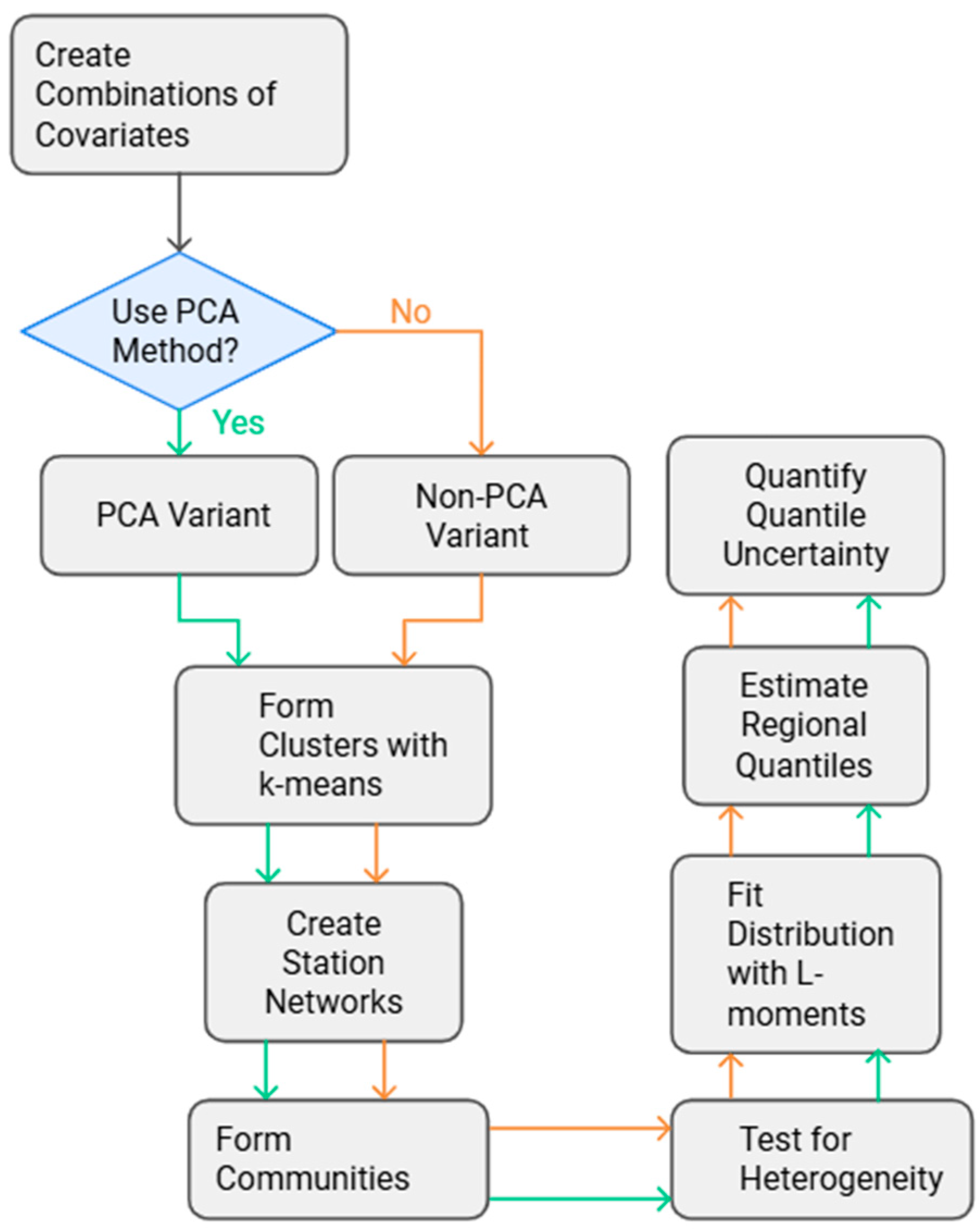
2.6. Methodology Application

Our method is divided into two different variants depending on whether we use the PCA method or not (Figure 2). Starting with the first step and using six station covariates (annual mean rainfall, longitude, latitude, elevation, mean maximum annual precipitation and l-skewness) we create every possible combination taking two to five at a time (56 different combinations). Next, with each of the covariate combinations, we apply the PCA method and choose the appropriate number of principal components that explain at minimum 90% of the total variance. In the next step, we take the rotations from the PCA variant and the scaled covariates from the non-PCA variant and we form clusters with the k-means. For every different input in the k means algorithm, we choose from two to seven different clusters. At this point, we have 280 different cluster formations in our region (in the PCA and in the non-PCA variants). After that, for every different number of clusters we form station networks. The connections are created so that the two stations are in the same cluster 50 out of the 56 times. The number is set arbitrarily by us so that with high confidence and independently of the covariates and the number of them the two stations will be in the same cluster. Next, using the igraph package v. 2.1.2 [90] in R programming language, we form communities maximizing the modularity measure. The communities formed are going to be the regions that will be tested with the heterogeneity measure and after that, the appropriate ones are going to be used for the regional frequency analysis. First, the best distribution is chosen with the Anderson–Darling goodness of fit tests and after that the distribution is fitted with L-moments [9]. Next the regional (with the index flood equation) and the InSite quantiles are estimated. Finally, the quantile uncertainty is quantified with parametric bootstrap.

3. Results

3.1. Multivariate Analysis and Clustering Results

As outlined in the introduction, our method has two variants based on the use of PCA. First, we generate all combinations of two to five station covariates (out of the six total: annual mean rainfall, longitude, latitude, elevation, mean annual maximum daily precipitation, and l-skewness), yielding 56 unique combinations. For each combination, we apply PCA and select the number of principal components that capture at least 90% of the variance. We then use the PCA rotations (PCA variant) or scaled covariates (non-PCA variant) as inputs to form two-to-seven clusters using the k-means algorithm. Station networks are subsequently constructed using at least two rainfall stations, linking stations that are in the same cluster at least 50 out of the 56 maximum combinations, and communities are identified by optimizing the modularity index.

Table 2. Communities formed using PCA for different k values used in the k-mean algorithm, evaluated with the H₁ heterogeneity measure.

PCA Variant
	C 1	C 2	C 3	C 4	C 5	C 6	C 7	C 8	C 9
k = 2	1.089	0.067	2.579	1.926	0.389	1.118
k = 3	0.438	2.846	2.055	1.027	0.158	0.543	0.928
k = 4	1.621	−1.047	0.318	1.748	−0.757	1.037	0.158	0.615	1.106
k = 5	0.797	−0.113	2.157	0.264	0.846	0.829	0.881	1.234
k = 6	2.021	−0.040	6.074	1.047
k = 7	1.981	0.334	0.999	0.968	0.619	1.170

and

Table 3. Communities formed using non PCA for different k value used in the k-mean algorithm, evaluated with the H1 heterogeneity measure.

Non PCA Variant
	C 1	C 2	C 3	C 4	C 5	C 6	C 7	C 8	C 9
k = 2	0.847	2.660	1.930	0.278	0.561	1.065
k = 3	0.442	3.142	1.915	0.867	0.120	0.601	6.071	1.075
k = 4	1.634	3.756	1.980	1.015	−0.820	−0.186	0.859	0.882
k = 5	0.788	−0.463	1.893	−0.285	0.270	0.919	0.870	1.011
k = 6	0.427	2.138	−0.815	0.283	1.131	1.560
k = 7	2.071	0.241	0.870	0.920	0.699	0.897

show the H₁ heterogeneity measure for each community. Rainfall stations that fail to satisfy the necessary membership condition are excluded from the subsequent analysis.

In Table 2, each row represents the communities formed at different cluster (k) levels, indicating that the composition of Community 3, for instance, varies across values of k. Our focus is thus on understanding the heterogeneity and structure of each unique community set within each k level. At k = 2, heterogeneity ranges widely, with Community 3 having the highest score (2.579) and Community 2 has the lowest (0.067). Communities 1, 4, 5, and 6 have intermediate values of 1.089, 1.926, 0.389, and 1.118, respectively. Community 4 has the most stations (13), while communities 5 and 6 each have only 2 stations. At k = 3, Community 2 has the highest score (2.846), followed by communities 3 (2.055) and 4 (1.027), with Community 5 scoring lowest (0.158). Community 3 has the most stations (11), while Community 6 has only 2. At k = 4, Community 1 has the highest heterogeneity (1.621), whereas communities 2 and 5 show negative values (−1.047 and −0.757). Community 1 has the highest station count (7), while communities 8 and 9 have just 2 stations each. For k = 5, 6, and 7, community properties remain relatively consistent, with station counts varying between 2 and 3, except for Community 2 at k = 6, which includes 5 stations. At k = 5, Community 3 has the highest heterogeneity (2.157), while Community 2 scores near zero (−0.113). At k = 6, Community 3 exhibits significant heterogeneity (6.074), while Community 2 is near zero (−0.040). At k = 7, Community 1 has the highest score (1.981), and Community 2 the lowest (0.334). Overall, the heterogeneity measure (H1) remains under 2 across most communities, suggesting acceptable homogeneity. The highest score (6.074) is seen in Community 3 at k = 6. Notably, the number of communities does not directly correspond to the number of clusters, with k = 4 showing a total of 9 communities. In contrast, as k increases, the total station count decreases, with 36 stations at k = 2.

In Table 3 we observe similar results with the non-PCA variants. At k = 2, Community 2 has the biggest value (2.660), while Community 4 has the smallest (0.278). Community 3 and Community 5 have moderate values of 1.93 and 0.561, respectively. Community 1 (14) and Community 3 (13) have the largest number of stations. At k = 3, Community 7 has the highest values, followed by Community 2, at 3.142. Community 5 has the smallest value of 0.120, and Community 3 has the biggest number of stations (11).At k = 4, Community 2 shows a high value of 3.756, while Community 5 has the smallest negative value (−0.820). Just as in the PCA variant, in the non-PCA variant for k = 5, 6, 7, the number of stations is 2–3. For k = 5, the highest value is 1.893, seen in Community 3. At k = 6, Community 2 shows the top value of 2.138. Lastly, at k = 7, the highest value is 2.071 in Community 1.

Both methods effectively form homogeneous station groups, with nearly identical communities created by both approaches.

Table 4. Rainfall station names and their total number in parentheses that form each Community for the PCA and Non PCA variants and k = 2.

	Station Names
PCA Communities		Non PCA Communities
C 1 (8)	Anavra, Agchialos, Makryraxh, Zileyto, Farsala, Magoyla, Skopia, Trilofo	C 1 (14)	Anavra, Agchialos, Zileyto, Farsala, Magoyla, Skopia, Myra, Farkadona, Elassona, Larisa, Tyrnavos, Karditsa, Swthrio, Zappeio
C 2 (8)	Myra, Farkadona, Elassona, Larisa, Tyrnavos, Karditsa, Swthrio, Zappeio
C 3 (7)	ElatiDEH, Agiofyllo, KipourgioKoniskos, Megalh_kerasia, Meteora, Pyloroi	C 2 (7)	ElatiDEH, Agiofyllo, Kipourgio, Koniskos, Megalh_kerasia, Meteora, Pyloroi
C 4 (13)	Drakotrypa, Amarantos, FragmaPlastira, Neoxori, Tymfristos, Argithea, ElatiYPEKA, Paleioxori, Chrysomilia, Moloha, Stoyrnaraiika, Vrontero, Malakasio	C 3 (13)	Drakotrypa, Amarantos, FragmaPlastira, Neoxori, Tymfristos, Argithea, ElatiYPEKA, Paleioxori, Chrysomilia, Moloha, Stoyrnaraiika, Vrontero, Malakasio
C 5 (2)	LivadiYPGE, LivadiYPEKA	C 4 (2)	LivadiYPGE, LivadiYPEKA
C 6 (2)	Redina, Pitsiota	C 5 (2)	Trilofo, Makryraxh
		C 6 (2)	Redina, Pitsiota

lists the rain gauges and their community assignments for $\mathrm{k}=2$. In the PCA variant, Communities 1 (Anavra, Agchialos, Makryraxh, Zileuto, Farsala, Mgoula, Skopia, Trilofo) and 2 (Myra, Farkadona, Elassona, Larisa, Tyrnavos, Karditsa, Soterio, Zappeio) merge to form Community 1 in the non-PCA variant, excluding two stations (Trilofo and Makryraxh), which belong to Community 5. In Figure 3 we see how the non-PCA communities are distributed in the study region. Since unified Community 1 offers a longer pooled record, we will use the first three communities from the non-PCA variant for the RFA method. This choice, as noted in the previous sections, enhances the reliability of high-quantile estimation.

3.2. Distribution Fitting

In this section, the results from the Anderson-Darling (AD) goodness of fit tests for the communities chosen are presented (

Table 5. Results from the AD goodness of fit test in the communities of the Non PCA variant.

	AD Test	Normal	Log-Normal	Generalized Extreme Value	P3	Generalized Pareto	GLO
C 1	A2	29.04	1.58	0.48	25.86	44.86	0.14
	P(A2)	1	0.98	0.86	1	1	0.03
C 2	A2	3.08	0.23	0.22	0.26	12.19	0.59
	P(A2)	1	0.41	0.38	0.37	1	0.95
C 3	A2	3.88	0.68	0.74	0.88	21.36	0.51
	P(A2)	1	0.98	0.99	0.99	1	0.91

). The results have been created with the NsRFA v. 0.7-17 [91] package in R. As stated in the documentation of the package, the P(A2) is one minus the p-value that the tests usually statistics use, meaning P(A2) is the probability of obtaining an AD score A2 smaller than the one observed. In the next paragraphs we will refer to this value as P. In the first community, the Log-Normal, Normal, P3 and GP distributions, their P score show strong evidence against the null hypothesis. The GEV distribution has a high P score and we cannot reject the null hypothesis. For this community, we will choose the GLO distribution since it has the lowest P score. For the second community the distributions Normal, GP and GLO with P scores 1, 1 and 0.95 are rejected for a level of 5%. For the distributions LN, GEV and P3 with P scores 0.41, 0.38, 0.37 we do not have enough evidence to reject the null hypothesis. In this community, even though the P3 distribution has a marginally better P score we are choosing the GEV distribution. The reason of this decision comes from the fact that according to classical extreme value theory [92], the GEV distribution has more solid theoretical foundation in describing block-maxima extreme random variables [81]. For the third community, the AD rejects all the distributions accept the GLO with P score of 0.91 where we cannot reject at significance level of 5%. The L-moment ratio diagram (Figure 4) validates the results from the AD test, and in

Table 6. Distribution parameters for the Non-PCA variant communities calculated with the L-moments.

	Xi	Alpha	Kappa
C 1-GLO	0.882	0.216	−0.296
C 2-GEV	0.845	0.286	0.040
C 3-GLO	0.967	0.168	−0.115

, the parameters of the fitted distributions with L-moments are presented.

In Figure 5, Figure 6 and Figure 7, regional cumulative distribution functions (CDFs) are shown alongside their InSite counterparts. In the InSite methodology, the same distribution is fitted to each station, consistent with the distribution selected for the pooled data of the Community to which each station belongs. The grey band represents the 5–95% confidence interval for the community’s average CDF, calculated by multiplying the growth curve by the mean of all records within the community. In Community 1, most regional and InSite CDFs fall within this confidence interval, while in the other two communities, quantile estimates across stations are more dispersed.

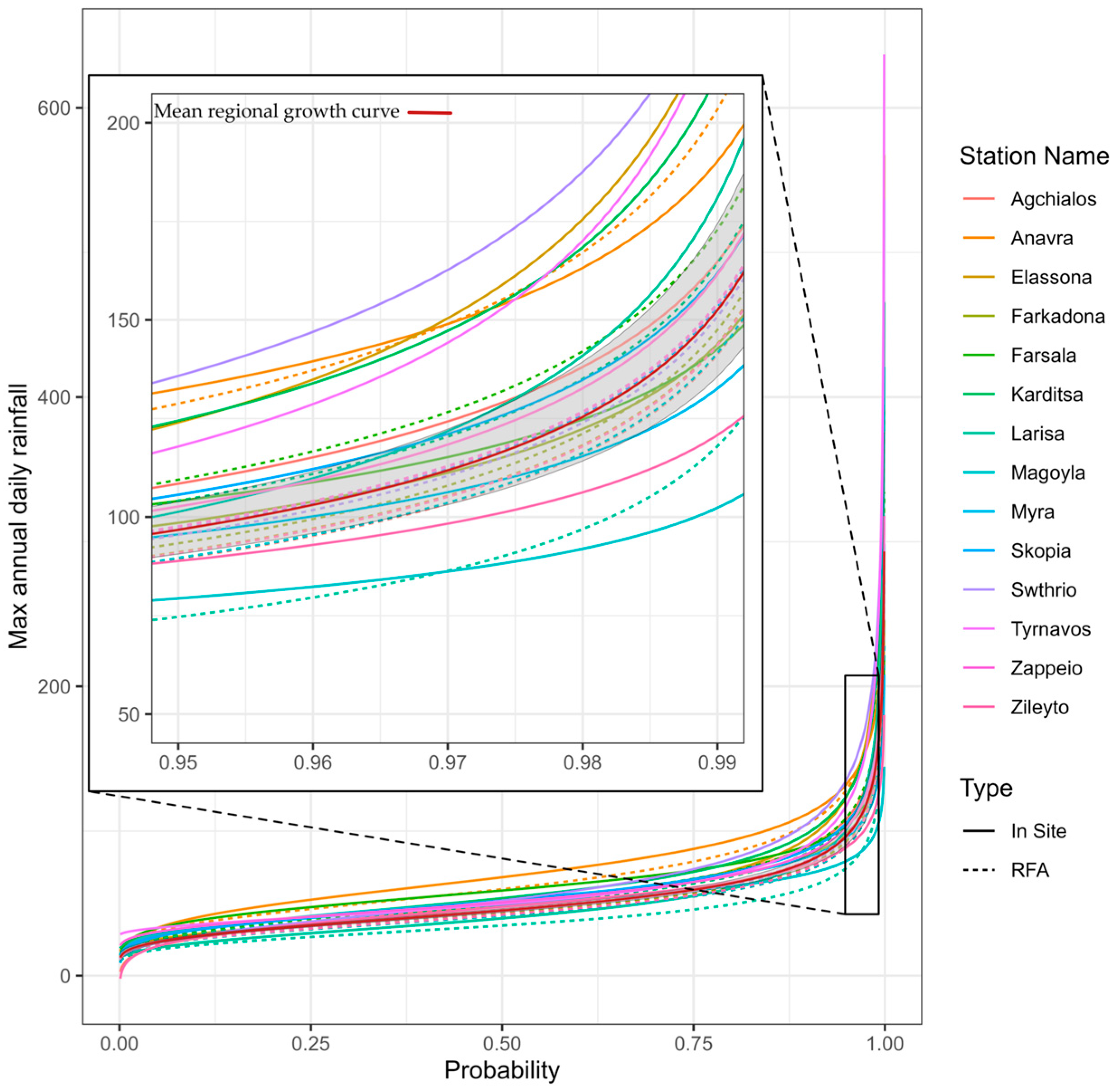
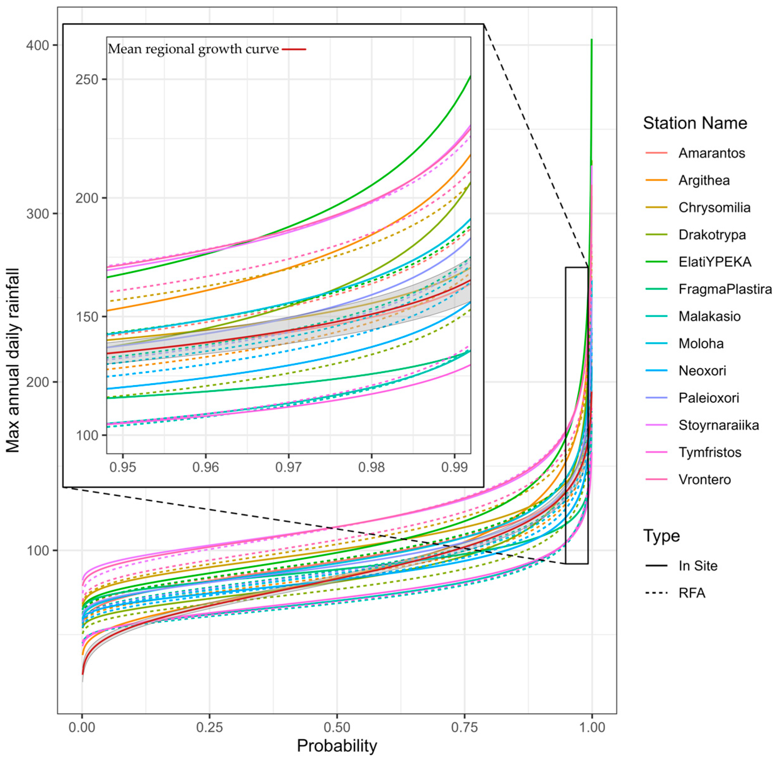
3.3. Quantile Estimation and Confidence Intervals

A deeper understanding of the previous figures can be gained by analyzing Figure 8, specifically for Community 1. This figure shows probability plots that compare two estimation methods, InSite and RFA, by displaying their distributions. The first notable observation is that both methods show an increase in values with higher quantiles, although the rate of increase differs. For instance, at the Zileyto and Magoula stations, the RFA curve rises more rapidly than the InSite curve, while the opposite occurs at the Swtirio and Larisa stations. The gray band in the figure represents the 5–95% confidence interval (CI), calculated using the parametric bootstrap method. It is important to note that, with both the RFA and InSite methods, we are working with finite data, meaning that the true parent distribution and true quantile values are unknown [93].

Furthermore, Figure 8 shows that some InSite quantiles fall within the RFA confidence intervals, while others do not. Due to sampling variability in both methods, comparing them requires evaluating their confidence intervals and specific quantile estimates. This study uses the T = 100 return period, commonly applied in hydrological infrastructure design.

In Figure 9 is presented the 5–95% confidence intervals calculated with the parametric bootstrap method for the RFA and InSite methodologies together with their estimation. In

Table 7. Summary characteristics of the RFA and InSite results for T = 100 years.

Communities		InSite 5–95% CI Range	RFA 5–95% CI Range	Absolute Error of Estimation
	Mean	122.46	57.14	32.17
C 1	Max	223.98	76.43	75.03
	Min	39.34	44.42	2.00
	Mean	45.63	19.37	15.84
C 2	Max	87.83	23.70	56.39
	Min	16.96	12.60	0.96
	Mean	73.59	25.41	21.87
C 3	Max	138.97	31.84	50.61
	Min	30.23	19.98	0.28

, some summary statistics are presented for the CI ranges and the Absolut error of estimation between the two methodologies.

Starting with InSite method, Community 1 has the highest average CI range at 122.46, compared to Communities 2 (45.63) and 3 (73.59). Community 1 also has the largest maximum range (223.98) in Tyrnavos station, followed by Community 3 (138.97) in Elati station and Community 2 (87.83) in Kokiniskos station. The minimum range in the InSite method is in Community 2 (16.96). For RFA method, Community 1 again appears to have the highest average range at 57.14, followed by Community 3 (25.41) and Community 2 (19.37). The maximum RFA CI range value in Community 1 (76.43) is also higher than in Community 3 (31.84) and Community 2 (23.70), respectively.

Turning to Absolute Error of Estimation, the results show Community 1 has the highest mean absolute error at 32.17, followed by Community 3 at 21.87 and with Community 2 having the lowest at 15.42. Similarly, the maximum (75.03) absolute error appears also in Community 1 in Swthrio station. In contrast, both Community 2 and Community 3 show minimum error values of around 0, implying cases with very accurate estimations. Community 1’s minimum error, at 2.00, suggests that even at its most accurate, some error remains. Finally we observe that the in all communities the Insite CI ranges are bigger that their RFA counterparts which is something we expect since we have a bigger number of data in the second method. Also, in all the communities there are stations that their inside estimation for T = 100 years don’t fall inside the RFA CI’s. Specifically, in Community 1 and 3 we have six stations and in Community 2 we have 3 stations. Overall, Community 1 appears to have the biggest sampling variability, with the highest values for InSite and RFA confidence intervals and estimation errors while Community 2, shows relatively low values for InSite and RFA, with narrow confidence intervals and the smallest absolute error.

4. Discussion

Extreme rainfall events are defined as occurrences over a specific period (annual, seasonal, or daily) where rainfall significantly exceeds the average for a given location. Understanding the probability of such events is crucial. These events are influenced by regional topography and dynamic factors [94]. Identifying homogeneous zones and clustering hydrometeorological variables are essential for studying extreme events [95].

Several studies incorporated PCA to study extreme rainfall [27,96,97,98]. For example, studies in Switzerland [20], Southeast Australia [99] and Italy [1] employed PCA combined with k-means to analyse extreme rainfall, reporting mixed success in identifying homogeneous regions. The challenges of achieving statistical homogeneity in RFA have been examined in the international literature. Hosking and Wallis’s seminal work on L-moments established a unified framework for RFA but relied heavily on predefined regional boundaries, which can introduce bias in heterogeneous landscapes [9]. Despite various approaches for identifying homogeneous regions, there is no guarantee that the resulting regions will be homogeneous [1,20,27,99,100,101,102]. For example, Pansera et al. [100], using monthly rainfall data from Paraná, Brazil, applied different clustering methods and found that, with their hierarchical algorithm, two of the six regions had heterogeneity measure $H_1=4.10 \& H_1=5.39$. Similarly, Jingyi and Hall [101] clustered 86 stations in southeastern China and found that one region had $H_1=2.71$. Dinpashoh et al. [27] divided Iran into six regions, one of which had $H_1=5.19$. Other studies, such as those by Forestieri et al. [1] and Gall et al. [20], report similar findings. Furthermore, a recent study from the authors in Thessaly area found that hydrological regions in Thessaly are heterogeneous when k-means clustering algorithms are combined with RFA (as proposed by Hosking and Wallis [9]) to analyse daily extreme rainfall [56]. In contrast, our method’s iterative clustering approach with network theory ensures statistically created homogeneous regions, as demonstrated in Thessaly’s complex terrain. Similar findings have been found in network theory application for delineation of homogenous regions in flood frequency analysis [49].

In the classical RFA method, the delineation of the area into homogenous regions is done by first selecting several appropriate variables. This choice is done a priori or by applying a preprocessing step, that analyses the significance of these variables. In the two-step network analysis, two main factors are considered, the similarity measure and the construction of the network. Our method tackles the subjectivity of the covariate selection by creating all possible clusters. Next, by combining all clusters and selecting the connections (edges) that appear in at least 50 out of the 56 possible covariate combinations (≈95% of occurrences) we create a similarity threshold measure. The two variants of our method (PCA and Non-PCA) are used to identify if PCA affects the network structure. PCA and Non-PCA network structure is presented in Figure 10 where similar spatial patterns are observed. This result is also verified by the modularity score, whereas PCA network and Non-PCA achieve modularity scores of 0.674 and 0.624, respectively. These results show that the homogenous regions in an RFA context also show strong community structure if a rainfall network is formed when the subjectivity of the covariates is removed. However, it should be noted that application of the method in other climatic areas could help to generalise the results of our study.

To understand implications of our findings, we compared the results from the our RFA method with the Greek national IDF curves [103] which are shown in Figure 11. In Community 1, both the RFA and IDF values are generally centered around 150 mm, with no clear trend observed. However, in Communities 2 and 3, the IDF values consistently overestimate rainfall, with Community 3 showing the largest overestimations. Additionally, positive trends are evident in the InSite estimations. These results highlight the limitations of relying solely on national IDF curves, which may not capture local rainfall variability accurately. Region-specific analyses, as demonstrated by our method, are crucial for improving design standards and risk assessments.

This study’s implications extend beyond Thessaly. The methodology can be applied to regions with similar data limitations or complex hydrological conditions. Integrating climate model projections into the clustering framework could further enhance its predictive capabilities. Future research could explore incorporating hydrological covariates, such as land-use changes or soil moisture indices, to refine homogeneous region definitions. Moreover, the scalability of the proposed approach allows for its adaptation to global hydrological challenges, including flood and drought frequency analyses. By addressing the uncertainties inherent in RFA, this study provides a robust framework for advancing water resource management and climate adaptation strategies on a broader scale.

5. Conclusions

This paper addresses the uncertainty associated with parameter selection in applying regional frequency analysis (RFA). Our methodology employs a “bottom-up” approach to reduce the subjectivity involved in covariate selection. By utilizing an iterative clustering process that considers all potential combinations of covariates, we establish a network in which stations are connected based on how frequently they co-occur in clusters throughout the process. Specifically, we propose a method to streamline decision-making when identifying statistically homogeneous regions, with two variants: one incorporating Principal Component Analysis (PCA) and the other without PCA. Starting with six station covariates (i.e., annual mean rainfall, longitude, latitude, elevation, mean maximum annual precipitation, and L-skewness) we generate all possible combinations of two to five covariates, totalling 56 combinations. For each, we apply PCA, selecting principal components that explain at least 90% of the variance. Next, we use either PCA rotations (for the PCA variant) or scaled covariates (for the non-PCA variant) as inputs to cluster data with the k-means algorithm, testing two to seven clusters per input. Using the igraph package in R, we form communities by maximizing the modularity index, identifying regions to assess for heterogeneity. After defining communities, we identify the best-fit distribution via the Anderson–Darling goodness-of-fit test, fit distributions using L-moments, and estimate both regional and InSite quantiles. Quantile uncertainty is calculated using parametric bootstrapping.

Our study area, Thessaly, includes annual maximum daily precipitation data from 55 rain gauges uniform distributed across the region. Results show that each variant of our method creates similar communities with the communities from k = 2 in k-means algorithm to be used in, further in our study. The AD test shows that the best distributions are the GEV, P3, and GLO. The estimation analysis for T = 100 years quantile between RFA and Insite shows that the Community 1 generally has the highest values, and the greatest variability compared to the Community 2 that exhibits the lowest and smallest values for all metrics, with tight confidence intervals and minimal estimation error. Community 3 falls between the other two with relative moderate values and variability. Finally, the estimates that come from the national IDF’s are explored. The results show, for Community one, a mix of overestimation and underestimation between IDF and RFA. In the other communities, we have a constant overestimation of the IDF values with positive trends to appear.

The proposed methodology could help the decision-making process for identifying homogeneous regions in extreme precipitation studies. It highlights the utility of clustering techniques combined with PCA in enhancing the robustness of covariate selection, ultimately leading to improved estimation of extreme precipitation quantiles under uncertainty. This approach is particularly useful for data scarce regions like Thessaly. Overall, this research contributes significantly to the field by providing a structured framework for dealing with parameter uncertainty in extreme precipitation modelling, emphasizing the importance of robust statistical methods in regional frequency analyses.

References

1. Forestieri, A.; Lo Conti, F.; Blenkinsop, S.; Cannarozzo, M.; Fowler, H.J.; Noto, L.V. Regional Frequency Analysis of Extreme Rainfall in Sicily (Italy). Int. J. Climatol. 2018, 38, e698–e716. [Google Scholar] [CrossRef]
2. Das, S.; Zhu, D.; Yin, Y. Comparison of Mapping Approaches for Estimating Extreme Precipitation of Any Return Period at Ungauged Locations. Stoch. Environ. Res. Risk Assess. 2020, 34, 1175–1196. [Google Scholar] [CrossRef]
3. Hailegeorgis, T.T.; Thorolfsson, S.T.; Alfredsen, K. Regional Frequency Analysis of Extreme Precipitation with Consideration of Uncertainties to Update IDF Curves for the City of Trondheim. J. Hydrol. 2013, 498, 305–318. [Google Scholar] [CrossRef]
4. Liang, Y.; Liu, S.; Guo, Y.; Hua, H. L-Moment-Based Regional Frequency Analysis of Annual Extreme Precipitation and Its Uncertainty Analysis. Water Resour. Manag. 2017, 31, 3899–3919. [Google Scholar] [CrossRef]
5. Bharath, R.; Srinivas, V.V. Regionalization of Extreme Rainfall in India. Int. J. Climatol. 2015, 35, 1142–1156. [Google Scholar] [CrossRef]
6. Dalrymple, T. Flood-Frequency Analyses, Manual of Hydrology: Part 3; U.S. Government Publishing Office: Washington, DC, USA, 1960. [Google Scholar]
7. Fundamentals of Statistical Hydrology; Naghettini, M., Ed.; Springer International Publishing: Cham, Switzerland, 2017; ISBN 978-3-319-43560-2. [Google Scholar]
8. Deidda, R.; Hellies, M.; Langousis, A. A Critical Analysis of the Shortcomings in Spatial Frequency Analysis of Rainfall Extremes Based on Homogeneous Regions and a Comparison with a Hierarchical Boundaryless Approach. Stoch. Environ. Res. Risk Assess. 2021, 35, 2605–2628. [Google Scholar] [CrossRef]
9. Hosking, J.R.M.; Wallis, J.R. Regional Frequency Analysis: An Approach Based on L-Moments; Cambridge University Press: Cambridge, UK, 1997; ISBN 978-0-521-43045-6. [Google Scholar]
10. Leščešen, I.; Šraj, M.; Basarin, B.; Pavić, D.; Mesaroš, M.; Mudelsee, M. Regional Flood Frequency Analysis of the Sava River in South-Eastern Europe. Sustainability 2022, 14, 9282. [Google Scholar] [CrossRef]
11. Prahadchai, T.; Busababodhin, P.; Park, J.-S. Regional Flood Frequency Analysis of Extreme Rainfall in Thailand, Based on L-Moments. Commun. Stat. Appl. Methods 2024, 31, 37–53. [Google Scholar] [CrossRef]
12. Zhang, Z.; Stadnyk, T.A. Investigation of Attributes for Identifying Homogeneous Flood Regions for Regional Flood Frequency Analysis in Canada. Water 2020, 12, 2570. [Google Scholar] [CrossRef]
13. Ghafori, V.; Sedghi, H.; Sharifan, R.A.; Nazemosadat, S.M.J. Regional Frequency Analysis of Droughts Using Copula Functions (Case Study: Part of Semiarid Climate of Fars Province, Iran). Iran. J. Sci. Technol. Trans. Civ. Eng. 2020, 44, 1223–1235. [Google Scholar] [CrossRef]
14. Li, M.; Liu, M.; Cao, F.; Wang, G.; Chai, X.; Zhang, L. Application of L-Moment Method for Regional Frequency Analysis of Meteorological Drought across the Loess Plateau, China. PLoS ONE 2022, 17, e0273975. [Google Scholar] [CrossRef] [PubMed]
15. Parvizi, S.; Eslamian, S.; Gheysari, M.; Gohari, A.; Kopai, S.S. Regional Frequency Analysis of Drought Severity and Duration in Karkheh River Basin, Iran Using Univariate L-Moments Method. Environ. Monit. Assess. 2022, 194, 336. [Google Scholar] [CrossRef] [PubMed]
16. Chen, X.; Zhu, D.; Wang, M.; Liao, Y. Regional Precipitation Frequency Analysis for 24-h Duration Using GPM and L-Moments Approach in South China. Theor. Appl. Clim. 2023, 152, 709–722. [Google Scholar] [CrossRef]
17. Fowler, H.J.; Kilsby, C.G. A Regional Frequency Analysis of United Kingdom Extreme Rainfall from 1961 to 2000. Int. J. Climatol. 2003, 23, 1313–1334. [Google Scholar] [CrossRef]
18. Jin, H.; Chen, X.; Zhong, R.; Duan, K. Frequency Analysis of Extreme Precipitation in Different Regions of the Huaihe River Basin. Int. J. Climatol. 2022, 42, 3517–3536. [Google Scholar] [CrossRef]
19. Mahmoudi, M.R.; Eslamian, S.; Soltani, S.; Tahanian, M. Regionalization of Rainfall Intensity–Duration–Frequency (IDF) Curves with L-Moments Method Using Neural Gas Networks. Theor. Appl. Clim. 2023, 151, 1–11. [Google Scholar] [CrossRef]
20. Gall, P.L.; Favre, A.-C.; Naveau, P.; Prieur, C. Improved Regional Frequency Analysis of Rainfall Data. Weather Clim. Extrem. 2022, 36, 100456. [Google Scholar] [CrossRef]
21. Nain, M.; Hooda, B.K. Regional Frequency Analysis of Maximum Monthly Rainfall in Haryana State of India Using L-Moments. J. Reliab. Stat. Stud. 2021, 14, 33–56. [Google Scholar] [CrossRef]
22. Ul Hassan, M.; Noreen, Z.; Ahmed, R. Regional Frequency Analysis of Annual Daily Rainfall Maxima in Skane, Sweden. Int. J. Climatol. 2021, 41, 4307–4320. [Google Scholar] [CrossRef]
23. García-Marín, A.P.; Morbidelli, R.; Saltalippi, C.; Cifrodelli, M.; Estévez, J.; Flammini, A. On the Choice of the Optimal Frequency Analysis of Annual Extreme Rainfall by Multifractal Approach. J. Hydrol. 2019, 575, 1267–1279. [Google Scholar] [CrossRef]
24. Srivastava, A.; Grotjahn, R.; Ullrich, P.A.; Risser, M. A Unified Approach to Evaluating Precipitation Frequency Estimates with Uncertainty Quantification: Application to Florida and California Watersheds. J. Hydrol. 2019, 578, 124095. [Google Scholar] [CrossRef]
25. Ibrahim, M.N. Assessment of the Uncertainty Associated with Statistical Modeling of Precipitation Extremes for Hydrologic Engineering Applications in Amman, Jordan. Sustainability 2022, 14, 17052. [Google Scholar] [CrossRef]
26. Hailegeorgis, T.T.; Alfredsen, K. Regional Flood Frequency Analysis and Prediction in Ungauged Basins Including Estimation of Major Uncertainties for Mid-Norway. J. Hydrol. Reg. Stud. 2017, 9, 104–126. [Google Scholar] [CrossRef]
27. Dinpashoh, Y.; Fakheri-Fard, A.; Moghaddam, M.; Jahanbakhsh, S.; Mirnia, M. Selection of Variables for the Purpose of Regionalization of Iran’s Precipitation Climate Using Multivariate Methods. J. Hydrol. 2004, 297, 109–123. [Google Scholar] [CrossRef]
28. Feidas, H.; Karagiannidis, A.; Keppas, S.; Vaitis, M.; Kontos, T.; Zanis, P.; Melas, D.; Anadranistakis, M. Modeling and Mapping Temperature and Precipitation Climate Data in Greece Using Topographical and Geographical Parameters. Theor. Appl. Climatol. 2013, 118, 133–146. [Google Scholar] [CrossRef]
29. Iliopoulou, T.; Malamos, N.; Koutsoyiannis, D. Regional Ombrian Curves: Design Rainfall Estimation for a Spatially Diverse Rainfall Regime. Hydrology 2022, 9, 67. [Google Scholar] [CrossRef]
30. Loukas, A.; Vasiliades, L. Streamflow Simulation Methods for Ungauged and Poorly Gauged Watersheds. Nat. Hazards Earth Syst. Sci. 2014, 14, 1641–1661. [Google Scholar] [CrossRef]
31. Vasiliades, L. Drought Spatiotemporal Analysis, Modelling and Forecasting in Pinios River Basin of Thessaly, Greece. Ph.D. Thesis, Department of Civil Engineering, School of Engineering, University of Thessaly, Volos, Greece, 2010. [Google Scholar]
32. Pereira, P.; Oliva, M.; Misiune, I. Spatial Interpolation of Precipitation Indexes in Sierra Nevada (Spain): Comparing the Performance of Some Interpolation Methods. Theor. Appl. Clim. 2016, 126, 683–698. [Google Scholar] [CrossRef]
33. Baeriswyl, P.-A.; Rebetez, M. Regionalization of Precipitation in Switzerland by Means of Principal Component Analysis. Theor. Appl. Clim. 1997, 58, 31–41. [Google Scholar] [CrossRef]
34. Burn, D.H. Evaluation of Regional Flood Frequency Analysis with a Region of Influence Approach. Water Resour. Res. 1990, 26, 2257–2265. [Google Scholar] [CrossRef]
35. Gaál, L.; Kysely, J.; Szolgay, J. Region-of-Influence Approach to a Frequency Analysis of Heavy Precipitation in Slovakia. Hydrol. Earth Syst. Sci. 2008, 12, 825–839. [Google Scholar] [CrossRef]
36. Guttman, N.B. The Use of L-Moments in the Determination of Regional Precipitation Climates. J. Clim. 1993, 6, 2309–2325. [Google Scholar] [CrossRef]
37. Hassan, B.G.H.; Ping, F. Regional Rainfall Frequency Analysis for the Luanhe Basin–by Using L-Moments and Cluster Techniques. APCBEE Procedia 2012, 1, 126–135. [Google Scholar] [CrossRef]
38. Lin, G.; Chen, L. Identification of Homogeneous Regions for Regional Frequency Analysis Using the Self-Organizing Map. J. Hydrol. 2006, 324, 1–9. [Google Scholar] [CrossRef]
39. Pineda-Martínez, L.F.; Carbajal, N.; Medina-Roldán, E. Regionalization and Classification of Bioclimatic Zones in the Central-Northeastern Region of México Using Principal Component Analysis (PCA). Atmósfera 2007, 20, 133–145. [Google Scholar]
40. Ramos, M.C. Divisive and Hierarchical Clustering Techniques to Analyse Variability of Rainfall Distribution Patterns in a Mediterranean Region. Atmos. Res. 2001, 57, 123–138. [Google Scholar] [CrossRef]
41. Santos, E.B.; Lucio, P.S.; Silva, C.M.S. e Precipitation Regionalization of the Brazilian Amazon. Atmos. Sci. Lett. 2015, 16, 185–192. [Google Scholar] [CrossRef]
42. Yang, T.; Shao, Q.; Hao, Z.-C.; Chen, X.; Zhang, Z.; Xu, C.-Y.; Sun, L. Regional Frequency Analysis and Spatio-Temporal Pattern Characterization of Rainfall Extremes in the Pearl River Basin, China. J. Hydrol. 2010, 380, 386–405. [Google Scholar] [CrossRef]
43. Hao, W.; Hao, Z.; Yuan, F.; Ju, Q.; Hao, J. Regional Frequency Analysis of Precipitation Extremes and Its Spatio-Temporal Patterns in the Hanjiang River Basin, China. Atmosphere 2019, 10, 130. [Google Scholar] [CrossRef]
44. Warren, R.A.; Jakob, C.; Hitchcock, S.M.; White, B.A. Heavy versus Extreme Rainfall Events in Southeast Australia. Q. J. R. Meteorol. Soc. 2021, 147, 3201–3226. [Google Scholar] [CrossRef]
45. Sivakumar, B. Networks: A Generic Theory for Hydrology? Stoch. Environ. Res. Risk Assess. 2015, 29, 761–771. [Google Scholar] [CrossRef]
46. Agarwal, A.; Marwan, N.; Ozturk, U.; Maheswaran, R. Unfolding Community Structure in Rainfall Network of Germany Using Complex Network-Based Approach. In Proceedings of the Water Resources and Environmental Engineering II; Rathinasamy, M., Chandramouli, S., Phanindra, K.B.V.N., Mahesh, U., Eds.; Springer: Singapore, 2019; pp. 179–193. [Google Scholar]
47. Kim, K.; Joo, H.; Han, D.; Kim, S.; Lee, T.; Kim, H.S. On Complex Network Construction of Rain Gauge Stations Considering Nonlinearity of Observed Daily Rainfall Data. Water 2019, 11, 1578. [Google Scholar] [CrossRef]
48. Han, X.; Ouarda, T.B.M.J.; Rahman, A.; Haddad, K.; Mehrotra, R.; Sharma, A. A Network Approach for Delineating Homogeneous Regions in Regional Flood Frequency Analysis. Water Resour. Res. 2020, 56, e2019WR025910. [Google Scholar] [CrossRef]
49. Joo, H.; Lee, M.; Kim, J.; Jung, J.; Kwak, J.; Kim, H.S. Stream Gauge Network Grouping Analysis Using Community Detection. Stoch. Environ. Res. Risk Assess. 2021, 35, 781–795. [Google Scholar] [CrossRef]
50. Rocha, R.V.; Souza Filho, F.D.A.D. Stream Gauge Clustering and Analysis for Non-Stationary Time Series through Complex Networks. J. Hydrol. 2023, 616, 128773. [Google Scholar] [CrossRef]
51. Newman, M.E.J. Networks, 2nd ed.; Oxford University Press: Oxford, UK; New York, NY, USA, 2018; ISBN 978-0-19-880509-0. [Google Scholar]
52. Fang, K.; Sivakumar, B.; Woldemeskel, F.M. Complex Networks, Community Structure, and Catchment Classification in a Large-Scale River Basin. J. Hydrol. 2017, 545, 478–493. [Google Scholar] [CrossRef]
53. Donges, J.F.; Zou, Y.; Marwan, N.; Kurths, J. Complex Networks in Climate Dynamics. Eur. Phys. J. Spec. Top. 2009, 174, 157–179. [Google Scholar] [CrossRef]
54. Newman, M.E.J. Analysis of Weighted Networks. Phys. Rev. E 2004, 70, 056131. [Google Scholar] [CrossRef] [PubMed]
55. Newman, M.E.J.; Girvan, M. Finding and Evaluating Community Structure in Networks. Phys. Rev. E 2004, 69, 026113. [Google Scholar] [CrossRef] [PubMed]
56. Mpillios, M.; Vasiliades, L. Regional Frequency Estimates of Annual Rainfall Maxima and Sampling Uncertainty Quantification. In Proceedings of the 8th International Electronic Conference on Water Sciences, Basel, Switzerland, 14–16 October 2024. [Google Scholar]
57. Loukas, A.; Mylopoulos, N.; Vasiliades, L. A Modeling System for the Evaluation of Water Resources Management Strategies in Thessaly, Greece. Water Resour Manag. 2007, 21, 1673–1702. [Google Scholar] [CrossRef]
58. Greenwood, J.A.; Landwehr, J.M.; Matalas, N.C.; Wallis, J.R. Probability Weighted Moments: Definition and Relation to Parameters of Several Distributions Expressable in Inverse Form. Water Resour. Res. 1979, 15, 1049–1054. [Google Scholar] [CrossRef]
59. Hosking, J.R.M. L-Moments: Analysis and Estimation of Distributions Using Linear Combinations of Order Statistics. J. R. Stat. Soc. Ser. B (Methodol.) 1990, 52, 105–124. [Google Scholar] [CrossRef]
60. Bayazit, M.; Önöz, B. Robustness Analysis of Regional Flood Frequency Models: A Case Study. In Coping with Floods; Rossi, G., Harmancioğlu, N., Yevjevich, V., Eds.; Springer: Dordrecht, The Netherlands, 1994; pp. 243–255. ISBN 978-94-011-1098-3. [Google Scholar]
61. Saf, B. Regional Flood Frequency Analysis Using L-Moments for the West Mediterranean Region of Turkey. Water Resour Manag. 2009, 23, 531–551. [Google Scholar] [CrossRef]
62. Zafirakou-Koulouris, A.; Vogel, R.M.; Craig, S.M.; Habermeier, J. L Moment Diagrams for Censored Observations. Water Resour. Res. 1998, 34, 1241–1249. [Google Scholar] [CrossRef]
63. Vogel, R.M.; Fennessey, N.M. L Moment Diagrams Should Replace Product Moment Diagrams. Water Resour. Res. 1993, 29, 1745–1752. [Google Scholar] [CrossRef]
64. Jolliffe, I.T. Principal Component Analysis; Springer Science & Business Media: New York, NY, USA, 2002; ISBN 978-0-387-95442-4. [Google Scholar]
65. Abdi, H.; Williams, L.J. Principal Component Analysis. WIREs Comput. Stat. 2010, 2, 433–459. [Google Scholar] [CrossRef]
66. Shlens, J. A Tutorial on Principal Component Analysis 2014. arXiv 2024, arXiv:1404.1100. [Google Scholar]
67. Ikotun, A.M.; Ezugwu, A.E.; Abualigah, L.; Abuhaija, B.; Heming, J. K-Means Clustering Algorithms: A Comprehensive Review, Variants Analysis, and Advances in the Era of Big Data. Inf. Sci. 2023, 622, 178–210. [Google Scholar] [CrossRef]
68. Steinley, D. K-Means Clustering: A Half-Century Synthesis. Br. J. Math. Stat. Psychol. 2006, 59, 1–34. [Google Scholar] [CrossRef]
69. Sahu, R.T.; Verma, M.K.; Ahmad, I. Regional Frequency Analysis Using L-Moment Methodology—A Review. In Proceedings of the Recent Trends in Civil Engineering; Pathak, K.K., Bandara, J.M.S.J., Agrawal, R., Eds.; Springer: Singapore, 2021; pp. 811–832. [Google Scholar]
70. Na, S.; Xumin, L.; Yong, G. Research on K-Means Clustering Algorithm: An Improved k-Means Clustering Algorithm. In Proceedings of the 2010 Third International Symposium on Intelligent Information Technology and Security Informatics, Jinggangshan, China, 2–4 April 2010; pp. 63–67. [Google Scholar]
71. Wang, J.; Su, X. An Improved K-Means Clustering Algorithm. In Proceedings of the 2011 IEEE 3rd International Conference on Communication Software and Networks, Xi’an, China, 27–29 May 2011; pp. 44–46. [Google Scholar]
72. Bock, H.-H. Clustering Methods: A History of k-Means Algorithms. In Selected Contributions in Data Analysis and Classification; Brito, P., Cucumel, G., Bertrand, P., de Carvalho, F., Eds.; Springer: Berlin/Heidelberg, Germany, 2007; pp. 161–172. ISBN 978-3-540-73560-1. [Google Scholar]
73. Newman, M.E.J. The Structure and Function of Complex Networks. SIAM Rev. 2003, 45, 167–256. [Google Scholar] [CrossRef]
74. Fortunato, S. Community Detection in Graphs. Phys. Rep. 2010, 486, 75–174. [Google Scholar] [CrossRef]
75. Javed, M.A.; Younis, M.S.; Latif, S.; Qadir, J.; Baig, A. Community Detection in Networks: A Multidisciplinary Review. J. Netw. Comput. Appl. 2018, 108, 87–111. [Google Scholar] [CrossRef]
76. Clauset, A.; Newman, M.E.J.; Moore, C. Finding Community Structure in Very Large Networks. Phys. Rev. E 2004, 70, 066111. [Google Scholar] [CrossRef]
77. Newman, M.E.J. Modularity and Community Structure in Networks. Proc. Natl. Acad. Sci. USA 2006, 103, 8577–8582. [Google Scholar] [CrossRef] [PubMed]
78. Girvan, M.; Newman, M.E.J. Community Structure in Social and Biological Networks. Proc. Natl. Acad. Sci. USA 2002, 99, 7821–7826. [Google Scholar] [CrossRef]
79. Brandes, U.; Delling, D.; Gaertler, M.; Gorke, R.; Hoefer, M.; Nikoloski, Z.; Wagner, D. On Modularity Clustering. IEEE Trans. Knowl. Data Eng. 2008, 20, 172–188. [Google Scholar] [CrossRef]
80. Viglione, A.; Laio, F.; Claps, P. A Comparison of Homogeneity Tests for Regional Frequency Analysis. Water Resour. Res. 2007, 43, W03428. [Google Scholar] [CrossRef]
81. Nguyen, T.-H.; El Outayek, S.; Lim, S.H.; Nguyen, V.-T.-V. A Systematic Approach to Selecting the Best Probability Models for Annual Maximum Rainfalls—A Case Study Using Data in Ontario (Canada). J. Hydrol. 2017, 553, 49–58. [Google Scholar] [CrossRef]
82. Hansen, C.R. Comparison of Regional and At-Site Frequency Analysis Methods for the Estimation of Southern Alberta Extreme Rainfall. Can. Water Resour. J./Rev. Can. Ressour. Hydr. 2015, 40, 325–342. [Google Scholar] [CrossRef]
83. Blanchet, J.; Ceresetti, D.; Molinié, G.; Creutin, J.-D. A Regional GEV Scale-Invariant Framework for Intensity–Duration–Frequency Analysis. J. Hydrol. 2016, 540, 82–95. [Google Scholar] [CrossRef]
84. Mascaro, G. Comparison of Local, Regional, and Scaling Models for Rainfall Intensity–Duration–Frequency Analysis. J. Appl. Meteorol. Climatol. 2020, 59, 1519–1536. [Google Scholar] [CrossRef] [PubMed]
85. Yue, S.; Hashino, M. Probability Distribution of Annual, Seasonal and Monthly Precipitation in Japan. Hydrol. Sci. J. 2007, 52, 863–877. [Google Scholar] [CrossRef]
86. Das, S. An Assessment of Using Subsampling Method in Selection of a Flood Frequency Distribution. Stoch. Environ. Res. Risk Assess. 2017, 31, 2033–2045. [Google Scholar] [CrossRef]
87. Das, S. Assessing the Regional Concept with Sub-Sampling Approach to Identify Probability Distribution for at-Site Hydrological Frequency Analysis. Water Resour. Manag. 2020, 34, 803–817. [Google Scholar] [CrossRef]
88. Laio, F. Cramer–von Mises and Anderson-Darling Goodness of Fit Tests for Extreme Value Distributions with Unknown Parameters. Water Resour. Res. 2004, 40, W09308. [Google Scholar] [CrossRef]
89. Kyselý, J. A Cautionary Note on the Use of Nonparametric Bootstrap for Estimating Uncertainties in Extreme-Value Models. J. Appl. Meteorol. Climatol. 2008, 47, 3236–3251. [Google Scholar] [CrossRef]
90. Gabor, C.; Tamas, N. The Igraph Software Package for Complex Network Research. Inter J. Complex Syst. 2006, 1695, 1–9. [Google Scholar]
91. Viglione, A. nsRFA: Non-Supervised Regional Frequency Analysis 2024. R Package Version 0.7-17. Available online: https://CRAN.R-project.org/package=nsRFA (accessed on 21 December 2024).
92. Coles, S. An Introduction to Statistical Modeling of Extreme Values; Springer Science & Business Media: New York, NY, USA, 2013; ISBN 978-1-4471-3675-0. [Google Scholar]
93. Schendel, T.; Thongwichian, R. Flood Frequency Analysis: Confidence Interval Estimation by Test Inversion Bootstrapping. Adv. Water Resour. 2015, 83, 1–9. [Google Scholar] [CrossRef]
94. Lima, A.O.; Lyra, G.B.; Abreu, M.C.; Oliveira-Júnior, J.F.; Zeri, M.; Cunha-Zeri, G. Extreme Rainfall Events over Rio de Janeiro State, Brazil: Characterization Using Probability Distribution Functions and Clustering Analysis. Atmos. Res. 2021, 247, 105221. [Google Scholar] [CrossRef]
95. Wilks, D.S. Chapter 13—Principal Component (EOF) Analysis. In Statistical Methods in the Atmospheric Sciences, 4th ed.; Wilks, D.S., Ed.; Elsevier: Amsterdam, The Netherlands, 2019; pp. 617–668. ISBN 978-0-12-815823-4. [Google Scholar]
96. Ngongondo, C.S.; Xu, C.-Y.; Tallaksen, L.M.; Alemaw, B.; Chirwa, T. Regional Frequency Analysis of Rainfall Extremes in Southern Malawi Using the Index Rainfall and L-Moments Approaches. Stoch. Environ. Res. Risk Assess. 2011, 25, 939–955. [Google Scholar] [CrossRef]
97. Jones, M.R.; Blenkinsop, S.; Fowler, H.J.; Kilsby, C.G. Objective Classification of Extreme Rainfall Regions for the UK and Updated Estimates of Trends in Regional Extreme Rainfall. Int. J. Climatol. 2014, 34, 751–765. [Google Scholar] [CrossRef]
98. Blenkinsop, S.; Fowler, H.J.; Dubus, I.G.; Nolan, B.T.; Hollis, J.M. Developing Climatic Scenarios for Pesticide Fate Modelling in Europe. Environ. Pollut. 2008, 154, 219–231. [Google Scholar] [CrossRef]
99. Ahmed, A.; Khan, Z.; Rahman, A. Searching for Homogeneous Regions in Regional Flood Frequency Analysis for Southeast Australia. J. Hydrol. Reg. Stud. 2024, 53, 101782. [Google Scholar] [CrossRef]
100. Pansera, W.; Gomes, B.; Boas, M.; Mello, E. Clustering Rainfall Stations Aiming Regional Frequency Analysis. J. Food Agric. Environ. 2013, 11, 877–885. [Google Scholar]
101. Jingyi, Z.; Hall, M.J. Regional Flood Frequency Analysis for the Gan-Ming River Basin in China. J. Hydrol. 2004, 296, 98–117. [Google Scholar] [CrossRef]
102. Chang, C.-H.; Rahmad, R.; Wu, S.-J.; Hsu, C.-T. Spatial Frequency Analysis by Adopting Regional Analysis with Radar Rainfall in Taiwan. Water 2022, 14, 2710. [Google Scholar] [CrossRef]
103. Koutsoyiannis, D.; Iliopoulou, T.; Koukouvinos, A.; Malamos, N.; Mamassis, N.; Dimitriadis, P.; Tepetidis, N.; Markantonis, D. Technical Report, Production of Maps with Updated Parameters of the Ombrian Curves at Country Level (Impementation of the EU Directive 2007/60/EC in Greece); Department of Water Resources and Environmental Engineering, National Technical University of Athens: Athens, Greece, 2023. [Google Scholar]
Figure 1. Map of the study area in Thessaly, Greece.
Water 17 00038 g001
Figure 2. Flow diagram of the methodology.
Water 17 00038 g002
Figure 3. Map of study region with the communities that are formed with the PCA and Non PCA variant.
Water 17 00038 g003
Figure 4. L–moment ratio diagram for the communities of the Non PCA variant.
Water 17 00038 g004
Figure 5. Regional and InSite CDF’s for the Community 1 formed with the Non-PCA variant.
Water 17 00038 g005
Figure 6. Regional and InSite CDF’s for the Community 3 formed with the Non-PCA variant.
Water 17 00038 g006
Figure 7. Regional and InSite CDF’s for the Community 2 formed with the Non-PCA variant.
Water 17 00038 g007
Figure 8. Community 1 CDF plots for of InSite estimation and RFA estimation together with the CI of the later.
Water 17 00038 g008
Figure 9. Diagram with the 5–95% CI’s of the RFA and InSite methodology together with their estimations for T = 100 years.
Water 17 00038 g009
Figure 10. (a) PCA and (b) Non-PCA network structure.
Water 17 00038 g010
Figure 11. Comparison between RFA and national IDF curve estimates for the T = 100 years quantile.
Water 17 00038 g011