Non-Point Source Pollution Risk Assessment in Karst Basins: Integrating Source–Sink Landscape Theory and Soil Erosion Modeling

Abstract

Non-point source pollution poses a significant threat to global water security, and risk assessment and key source area (CSA) identification are critical for its management. While source–sink landscape models are widely used for non-point source pollution evaluation, their application in karst regions is challenged by ecological fragility, shallow soil layers, and severe soil erosion, limiting their effectiveness in accurately identifying pollution risks and CSAs. This study focuses on the Caohai Lake basin in southwestern China; it integrates the landscape-weighted load index (LWLI) and the universal soil loss equation (USLE) to assess non-point source pollution risks in the basin with the aim of precisely delineating critical source areas (CSAs). Total phosphorus (TP) and total nitrogen (TN) served as key predictors of water quality, and their responses to the LWLI and USLE were analyzed in the karst environment. The results revealed the following: (1) source landscapes cover 65% of the basin area, with cropland (40%) being the primary contributor to nitrogen pollution; (2) the LWLI and USLE explain 50–67% of the TP and TN variations during the wet season, with a sharp increase in water quality risk when the LWLI exceeds 0.75; and (3) high-risk and very high-risk areas account for 36.3% and 15.3% of the basin, respectively, and are concentrated in the northwest and south, where intensive agriculture and severe soil erosion dominate. These findings provide a scientific basis for non-point source pollution control in the Caohai Lake basin.

1. Introduction

NPS pollution represents a significant global environmental challenge, severely compromising water quality and threatening water resource security [1,2,3,4,5]. NPS affects 30–50% of global water bodies, with nitrogen (N) and phosphorus (P) pollution contributing to over 50% [6]. According to the U.S. Environmental Protection Agency, five of the six primary sources of watershed pollution stem from NPS [7]. In the European Union and Germany, agriculture accounts for 55% and 48% of NPS, respectively [8]. Similarly, in China, over 60% of TP discharge in the Yellow River basin and nearly 50% of N and P pollution in the Yangtze River basin come from agricultural NPS [9]. Non-point source (NPS) pollution can be categorized into urban and rural NPS pollution. In particular, rural NPS pollution is characterized by a broader range of sources and more complex mechanisms, making monitoring difficult and its prevention and control challenging [10,11]. Therefore, accurately identifying key source areas for NPS pollution is a critical step in developing effective prevention and control strategies [12].

Currently, commonly used hydrological models, such as SWAT [13,14] and AGNPS [15], are used to identify CSAs at the watershed scale. However, these models have certain limitations in the analysis of the mechanisms and processes of surface source pollution. Additionally, they lack the capability to integrate nutrient monitoring data with the ecological processes of non-point source pollution, which restricts the precision of risk assessment and the accurate identification of CSAs at the watershed scale. In recent years, the source–sink theory has been introduced into landscape ecology to evaluate NPS risks at the regional or watershed scales [16]. In this context, source refers to the landscape types that promote ecological processes, while sink refers to the types that inhibit them. When the intensity of source landscapes exceeds that of sink landscapes, more pollutants are released, increasing the pollution risk [17,18]. The “source–sink” model integrates landscape patterns and nutrient loss data to effectively elucidate the relationship between landscape configuration and pollutant migration while assessing non-point source (NPS) pollution risks at the regional or watershed scales. However, in certain unique geological and geomorphological regions, traditional “source–sink” simulations that incorporate landscape types, area, spatial distribution, and topographic features often fail to accurately characterize NPS pollution. For instance, in karst ecosystems, biogeochemical processes exhibit high spatial and temporal heterogeneity. Severe soil erosion, shallow soil layers, and extensive exposed bedrock exacerbate soil loss, leading to intensified erosion and substantial variability in pollutant transport and migration processes [19]. Moreover, soil conditions and rainfall further intensify pollution risks [20]. Dissolution channels in karst geomorphology play a crucial role in material transport during soil erosion, runoff, and pollutant infiltration processes [21]. These channels, combined with rapid groundwater flow, facilitate the swift transfer of key eutrophication-inducing pollutants, such as P and N, significantly increasing the risk of pollution diffusion [22,23]. Additionally, frequent human activities further exacerbate ecological stress in karst regions [24]. Therefore, it is essential to develop an indicator system tailored to the unique characteristics of karst regions to effectively represent non-point source pollution risks and guide regional management efforts.

This study focuses on the Caohai Lake basin, a typical karst plateau wetland ecosystem in southwestern China; this basin is facing increasingly severe non-point source pollution threats. Although numerous studies have applied the source–sink landscape model to assess non-point source pollution in basins, the traditional methods face limitations when addressing the unique characteristics of karst basins. Based on the spatial attributes of source–sink landscapes and the soil erosion characteristics of karst areas, this study adopts a combined approach using both the LWLI and the USLE to improve the precision of CSA identification for non-point source pollution. Additionally, ecological processes are integrated with actual monitoring data. By using TP, TN, and other water quality indicators as predictive variables for the LWLI and USLE, the study assesses the impact of spatial heterogeneity in the karst environment on TP and TN levels. The objectives of this study are as follows: (1) to determine the spatial distribution trends of the LWLI in the Caohai Lake basin and to evaluate the key threshold values for water quality changes; (2) to identify and analyze the spatial distribution and characteristics of key source areas for non-point source pollution in the basin; and (3) to reveal the coupling relationship between the LWLI, soil erosion, and water quality (TP, TN). Through these efforts, the study aims to provide scientific evidence for non-point source pollution risk assessment and key source area identification in the Caohai Lake basin, and to offer targeted strategy recommendations for basin management and ecological restoration.

2. Materials and Methods

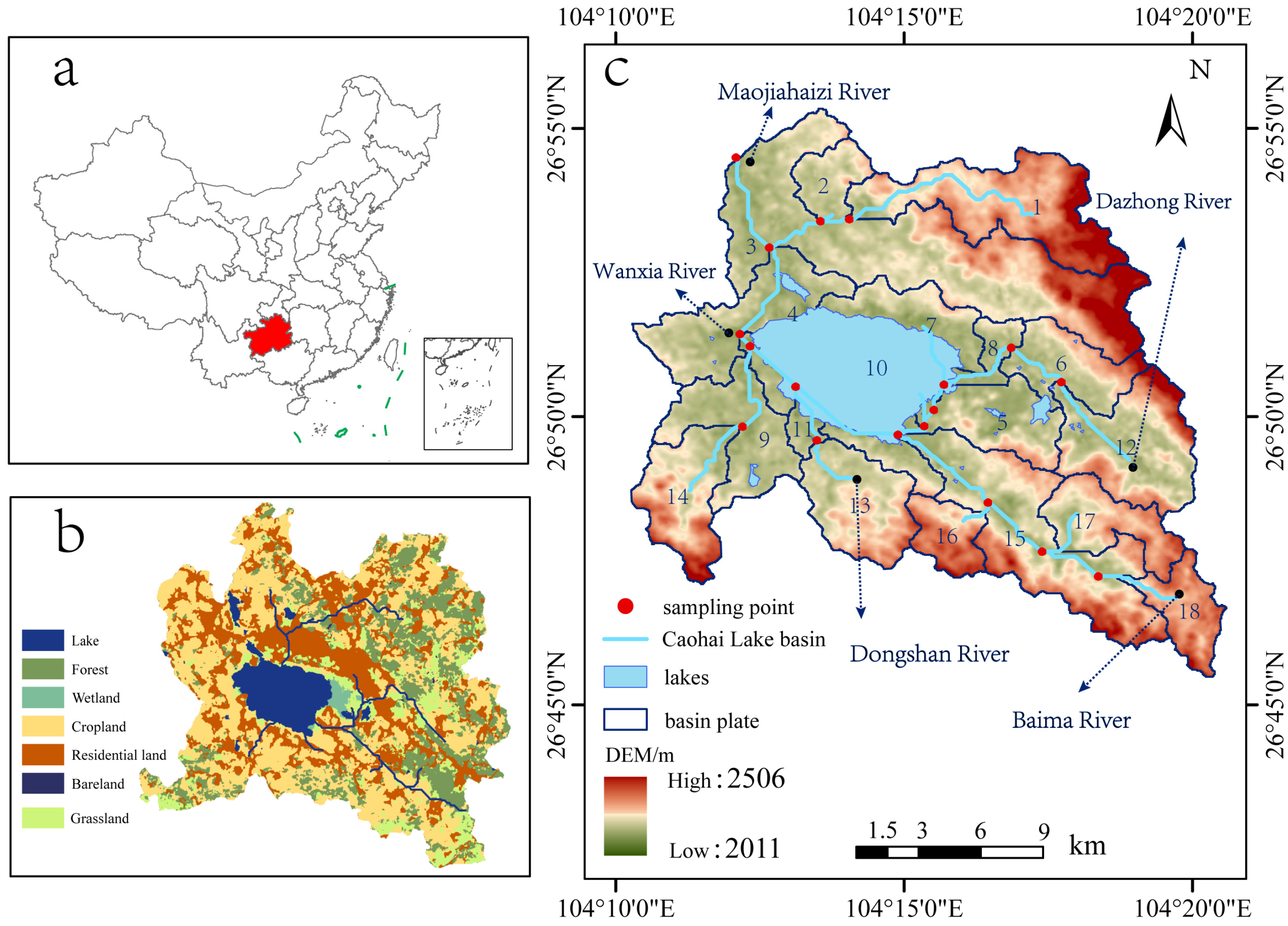
2.1. Study Area Overview

Caohai Lake is located in Weining County, western China (26°85′24″ N, 104°22′59″ E), in a subtropical plateau monsoon climate zone. This region experiences abundant sunshine, mild winters, and cool summers, along with distinct seasonal precipitation patterns, including dry winters and wet summers. Annual rainfall typically ranges from 900 to 1200 mm; the precipitation is primarily concentrated between May and August and accounts for 70.4% of the yearly total [25]. The landscape of this region is shaped by tectonic activity, lithological variations, and long-term erosion–dissolution processes, resulting in a typical karst landform with elevated areas surrounding a relatively flat central basin. This unique karst geomorphology affects local hydrological processes, enhances water infiltration, and accelerates material transport. The main rivers in the basin include the Dazhong River, Maojiahai River, Dongshan River, Baima River, and Wanxia River, all of which emanate from the central basin and ultimately drain into Caohai Lake (Figure 1). The topography is characterized by higher elevations in the southwest and lower elevations in the north. Water typically flows through the northwestern outlet into Suohuangcang National Wetland Park and eventually converges with the Luoze River, a tributary of the Jinsha River. This distinctive topographical structure forms unique pathways and patterns for water and pollutant transport, complicating the migration of NPS pollution within the basin. The karst terrain amplifies the infiltration of water and facilitates the movement of pollutants, making pollution management in the Caohai Lake basin particularly challenging.

2.2. Sample Collection and Processing

To effectively assess the pollution risks in the Caohai Lake basin, this study utilized the 2022 administrative boundary plan of China, along with the topographic and geomorphological characteristics of the basin. Using the SWAT model, the watershed was divided into 18 sub-basins. Water quality monitoring was subsequently conducted for these sub-basins during the dry season (April 2024) and wet season (August 2024), with one sampling point designated in each sub-basin. On-site water quality parameters, including water temperature, turbidity, pH, dissolved oxygen (DO), electrical conductivity (EC), and oxidation–reduction potential (ORP), were measured using a YSI Pro DSS multiparameter water quality analyzer. Water samples were collected in 250 mL polyethylene bottles and transported to the laboratory within 24 h for chemical analysis. The concentrations of TP and TN were determined using the persulfate oxidation ultraviolet spectrophotometry and ammonium molybdate spectrophotometry methods, respectively. Surface water samples were collected from the outlets of 18 sub-basins within the study area. All water quality parameters were analyzed in triplicate using subsamples. The final concentrations were calculated by taking the arithmetic mean of the two subsamples with differences of less than 5% and subtracting the blank sample values to ensure accuracy and reliability.

2.3. NPS Pollution Risk Assessment Based on the Source–Sink Theory

This study employed the LWLI to quantitatively describe the relationship between the spatial configuration of landscape elements and nutrient loss [26]. The Lorenz curve was applied to analyze the relative distance, elevation, and slope between landscape units and watershed outlets, providing a quantitative evaluation of how source–sink landscape patterns influence nutrient loss [27]. TP and TN concentrations were identified as critical factors of NPS pollution, and the LWLI was used to assess the retention capacity for TP and TN in the watershed, as well as the associated pollution risks [28]. By accounting for the interactions between the source and sink landscapes, the landscape spatial load index in the basin could be calculated using the following equations:

$$LWLI={\displaystyle \frac{{\sum }_{i=1}^n{A}_{{source}_i }\times { W}_{i }\times { AP}_i}{{\sum }_{i=1}^n{A}_{{source}_i} {\times W}_i{\times AP}_i+{\sum }_{j=1}^m{A}_{{sink}_j}{\times W}_j\times { AP}_j}}$$

(1)

where $LWLI$ is the location-weighted landscape load index based on N and P relative to the sub-basin’s outlet sampling point. $A_{{source}_i} \mathrm{a}\mathrm{n}\mathrm{d} A_{{sink}_j}$ represent the areas of the Lorenz curve for the “source” landscape $i$ and “sink” landscape $j$, respectively, in relation to relative elevation, slope gradient, or distance. $W_i$ and $W_j$ are the weights of the “source” landscape $i$ and “sink” landscape $j$, respectively. ${AP}_i$ and ${AP}_j$ represent the area proportions of the “source” landscape $i$ and “sink” landscape $j$ within the sub-basin, respectively. $m$ and $n$ denote the number of “source” and “sink” landscape types, respectively. If the effects of relative elevation, slope gradient, and distance on NPS pollution are combined, the index can be described as follows:

$$LWLI={\displaystyle \frac{{{LWLI}^{\prime }}_{distance}\times {{LWLI}^{\prime }}_{elevation}}{{{LWLI}^{\prime }}_{slope}}},$$

(2)

where ${{LWLI}^{\prime }}_{distance}$, ${{LWLI}^{\prime }}_{elevation}$, and ${{LWLI}^{\prime }}_{slope}$ are the values of the LWLI with respect to distance, relative elevation, and slope gradient, respectively.

Subsequently, the weight coefficients for the key indicators of TP and TN in the Caohai Lake basin could be calculated using the 2022 Caohai Lake Ecological Monitoring Report (Table S1). Using the LWLI formula, the landscape-weighted load indices for TP and TN were determined for the 18 sub-basins.

2.4. Identification Method of CSA for NPS Pollution

Based on the source–sink theory, which is used assess the effect of different landscape types on regional ecological processes, spatial overlay analysis was conducted, integrating soil erosion and land use types in the basin. To eliminate the interference of different dimensional factors, standardization was applied to various factors, such as soil erosion, landscape spatial load, and land use types. The soil erosion rate was subsequently calculated using the USLE model, while the land use types were empirically assigned according to previous research [29]. The standardized factors were then multiplied by their respective weights and summed. The natural breaks method was used to classify the results and to identify CSAs for NPS pollution within the basin. The purpose of standardization was to convert the different dimensional factors to the same scale, using the following min–max normalization formula:

$$X^{\prime }={\displaystyle \frac{x-x_{min}}{x_{max}-{ x}_{min}}},$$

(3)

where $X^{\prime }$ is the standardized value (i.e., LWIL′, USLE′, and LU′), $x$ is the original value, and $x_{max}-x_{min}$ denote the minimum and maximum values of the factor, respectively. The final NPS pollution risk value was represented by the CSA, which was calculated using the following formula:

$$\mathrm{C}\mathrm{S}\mathrm{A}={\sum }_{i=1}^3{W}_i\times {X^{\prime }}_i,$$

(4)

where $W_i$ is the weight of the i-th factor ($W_{LWIL}$ = 0.4, $W_{USLE}$ = 0.4, and $W_{LU}$ = 0.2), and $X_i$ is the standardized value of the i-th factor.

2.5. Statistical Analysis and Data Processing

This study used three types of spatial data for analysis: (1) the digital elevation model (DEM) with a resolution of 30 m, which was obtained from the Geospatial Data Cloud Platform of the Chinese Academy of Sciences (http://www.gscloud.cn; accessed on 9 March 2024); (2) land use data for 2022, derived from the global Sentinel-2 land cover product (https://creativecommons.org/licenses/by/4.0/; accessed on 2 February 2024) [30]; and (3) the “China 30 m Resolution Soil Erosion Intensity Dataset”, covering 9 periods from 1981 to 2020, which was provided by the Chengdu Institute of Mountain Hazards and Environment, Chinese Academy of Sciences. (released on 24 August 2024) [31]. Spatial data analysis was conducted using Excel 2022, and ArcMap 10.7 was used to extract land use areas across different elevations, distances, and slopes. Frequency histograms, cumulative distribution graphs, and cumulative area curves were generated and calculated using Python version 3.9.13. ArcMap 10.7 software was also used to visualize the relevant factors.

Non-parametric change-point analysis (nCPA) was applied to identify the thresholds of the landscape LWLI that corresponded to abrupt changes in water quality. The deviance reduction method was used to determine the optimal change-points by evaluating data homogeneity, allowing the response variables to be divided into distinct groups. Subsequently, the bootstrap simulation method was employed to estimate the frequency distribution of the change points, ensuring the reliability of threshold identification. These nCPA analyses were conducted using the “rpart” and “boot” functions in the R version 4.2.2. software environment [32,33]. Furthermore, data processing and plotting were performed using Origin 2022 and Chiplot (https://www.chiplot.online/; accessed on 29 August 2024) software.

3. Results

3.1. Landscape Characteristics of the Karst Basin

The spatial landscape load demonstrates how “source–sink” landscapes contribute to pollutant outputs at sub-basin outlets. “Source” landscapes, including croplands, urban areas, and bare land, accounted for 65% of the total basin area (23,775 hectares), while “sink” landscapes, such as forests, wetlands, lakes, and grasslands, constituted 35% (10,165 hectares). The accuracy of the land use classification was validated, showing an overall classification accuracy of 91% and a Kappa coefficient of 0.88 (

Table 1. Land use types, area, and accuracy assessment.

	Land Use Type	Area (hm2)	User Accuracy	Producer Accuracy
Sink landscapes	Wetland	269	81.81%	84.37%
	Forest	6544	92.72%	96.22%
	Grassland	3352	86.50%	82.35%
	Lake	2497	86.36%	79.16%
Source landscapes	Cropland	14,211	95.10%	91.80%
	Residential land	9539	90.78%	94.52%
	Bare land	25	75.00%	75.00%
Kappa coefficient: 0.88		Overall accuracy: 91%

Note: Kappa coefficient measures classification accuracy from 0 to 1, where higher values indicate better accuracy; it is especially useful for small samples. Overall accuracy is the percentage of correctly classified land use types, with higher values indicating better quality. User accuracy indicates how accurately each land use type was identified. Producer accuracy indicates consistency between classification and actual land use types.

), which indicated high reliability for further analysis and research. Using the Lorenz curve theory, the cumulative areas of the “source” and “sink” landscapes were calculated based on relative elevation, distance, and slope (Figures S1–S3). Spatially, the low-elevation areas were predominantly composed of “sink” landscapes, including grasslands, wetlands, and lakes. In contrast, the regions with gentle slopes and flat elevations were dominated by “source” landscapes, such as croplands and residential areas. The forests were primarily distributed in areas with higher elevations and steeper slopes. From a relative distance perspective, sub-basins 2, 9, 12, and 13 exhibited “source” landscapes closer to basin outlets, suggesting that these areas may contribute more significantly to NPS pollution over shorter distances. The slope analysis indicated that the “source” landscape units were primarily distributed in areas with gentle slopes, where the risk of nutrient loss was relatively low. Conversely, the “sink” landscapes were more frequently located in steeper areas, effectively intercepting nutrient loss and mitigating pollution risks [34]. Thus, the spatial analysis of the “source–sink” landscapes in the Caohai Lake basin highlights the significant pollution contribution potential of “source” landscapes, particularly with regard to elevation and distance from basin outlets.

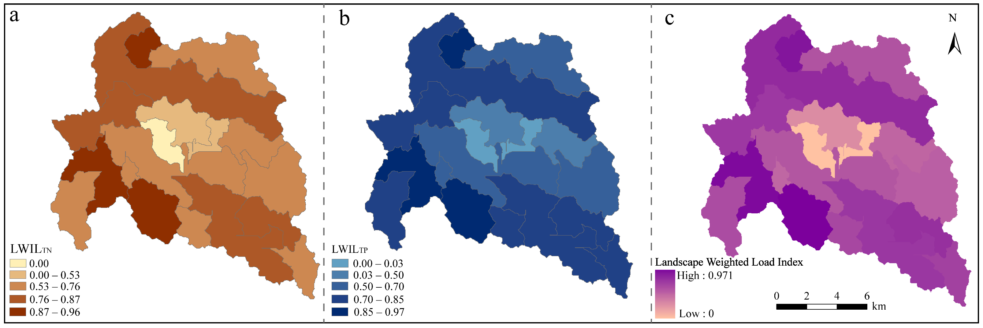
3.2. Spatial Risk Assessment of “Source–Sink” Landscapes in the Karst Basin

The spatial landscape load reveals the potential contribution of “source–sink” landscapes to pollutant outputs at sub-basin outlets. In the Caohai Lake basin, the LWLI was calculated using the weighted average method, yielding an average value of 0.69. More than half of the sub-basins had LWLI values exceeding this average, indicating that the contribution of the “source” landscapes to pollutant outputs at the outlets was significantly higher than the pollution reduction capacity of the “sink” landscapes. This imbalance underscores the high spatial pollution load potential across the entire basin. Specifically, the LWLI_TP and LWLI_TN values ranged from 0 to 0.97, with average values of 0.68 and 0.70, respectively (Figure 2a,b). After integrating the weighted contributions of the TP and TN loads, the LWLI values across the basin ranged from 0 to 0.97. Notably, sub-basins 2, 9, and 13 exhibited LWLI values of approximately 0.90, indicating extremely high landscape spatial loads (Figure 2c). In these high-load areas, the “source” landscapes accounted for up to 75% of the total landscape composition, significantly exceeding the proportion of “sink” landscapes. These areas are primarily concentrated in the northwestern, southwestern, and southeastern parts of the basin and have substantial pollution impacts on the Dongshan River, Wanxia River, and Baima River.

Using a non-parametric method, the frequency histogram and cumulative distribution of the LWLI change point locations were calculated, revealing the frequency distribution of TP and TN at different LWLI values and their cumulative threshold trends (Figure 3). Furthermore, a mutation analysis of the LWLI at the basin scale was conducted. When the LWLI value exceeds 0.75, the cumulative probability of TP and TN concentrations exceeds 60%. This indicates that when the LWLI reaches 0.75, it marks a significant increase in TP and TN concentrations at this threshold. Within the sub-basins, the “source” landscape, due to its higher nutrient output capacity, surpasses the interception and absorption capacity of the “sink” landscape. This imbalance exacerbates nutrient loss, leading to a substantial influx of N and P pollutants into the water, significantly increasing the water quality risk.

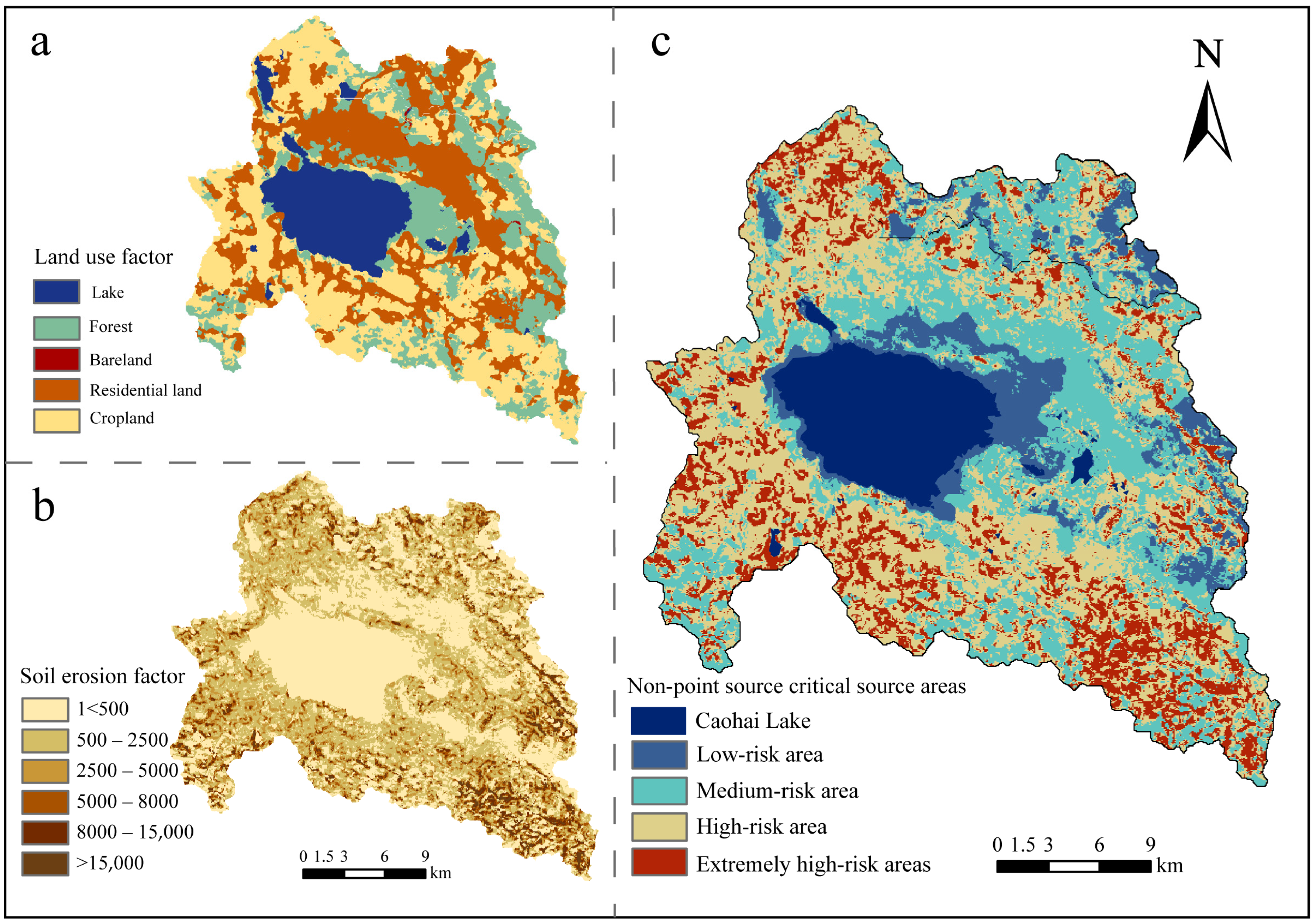
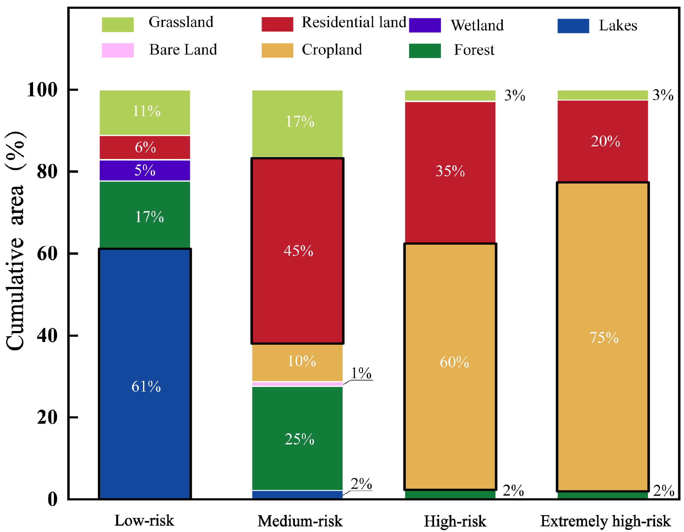
3.3. Identification and Composition of Critical Source Areas (CSAs) in the Karst Basin

Land use and soil erosion intensity emerge as key factors influencing CSA distribution (Figure 4). Land use type factors are categorized into four levels: Level 1 (forest, grassland, and wetland), Level 2 (bare land and lakes), Level 3 (residential areas), and Level 4 (cropland) (Figure 4a). The spatial distribution of soil erosion intensity (Figure 4b) reveals that mild (32%) and moderate (15%) erosion predominate in the basin, while areas of severe, very severe, and extreme erosion collectively account for 11% and are primarily concentrated in the southeastern part of the basin. These regions of high erosion often overlap with areas exhibiting elevated LWLI values, underscoring their critical role in contributing to the NPS pollution risk.

The spatial distribution of critical source areas (CSAs) for NPS pollution in the Caohai Lake basin exhibits significant spatial heterogeneity. Using a combination of functional landscape classification, soil erosion intensity analysis, and the landscape LWLI, the natural breaks method was employed to classify the NPS pollution risk indices, delineating the spatial distribution and landscape composition of the CSAs. The results indicate that high-risk areas (36.25%) and extremely high-risk areas (15.28%) together account for 52% of the basin’s total area and are predominantly located in the southern and northwestern regions of the basin. These zones, which are characterized by high soil erosion intensity and elevated LWLI values, represent critical areas for NPS pollution control. Conversely, medium-risk and low-risk areas constitute 48% of the basin’s total area and are primarily situated in the central and lakeside regions, where pollution mitigation capacity is relatively strong, resulting in lower overall risk.

The analysis of landscape structures across different risk areas reveals distinct spatial patterns. The low-risk areas are primarily distributed near the Caohai Lake, where sink landscapes account for 94% of the total area, with lakes constituting 61% and wetlands 5% (Figure 5). As key sink landscapes, lakes and wetlands significantly reduce the loss of N and P, thereby effectively lowering NPS pollution loads. Additionally, these areas exhibit low soil erosion intensity, which is predominantly characterized by mild or minimal erosion, further mitigating pollution risks. In medium-risk areas, the landscape structure is relatively balanced, with sink and source landscapes accounting for 45% and 55% of the area, respectively. The key sink landscape types include forests, grasslands, wetlands, and lakes, all of which demonstrate strong pollutant interception capacity. Source landscapes in these regions primarily consist of croplands and residential areas, with residential areas contributing 45% and serving as a major source of NPS pollution. Although the pollution risks in these areas are higher than in low-risk regions, the regulatory functions of sink landscapes help maintain pollution levels within a moderate range. High-risk and extremely high-risk areas exhibit significant landscape imbalance, with source landscapes dominating the region. Cropland accounts for 60–70% of these areas, while residential areas contribute an additional 20–35%. These zones experience high soil erosion intensity, particularly in the southeastern and northwestern parts of the basin, overlapping with areas of elevated LWLI values. The insufficient coverage of sink landscapes in these regions hinders the effective mitigation of pollution loads from source landscapes, leading to a marked increase in NPS pollution. The high proportion of agricultural activities and residential expansion is the primary driver of elevated pollution risks in these areas.

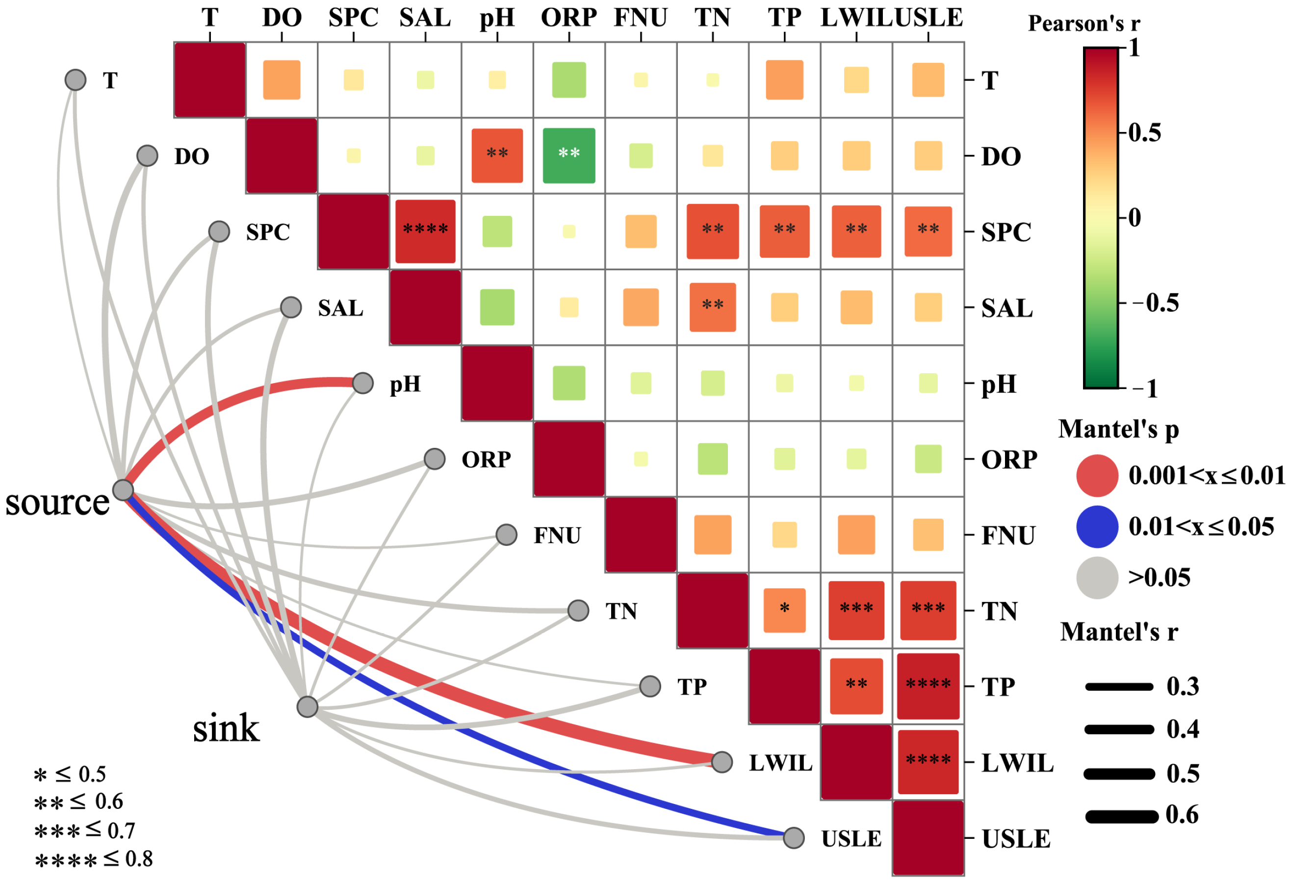
3.4. Coupling Relationships Between CSA Key Factors and Basin Water Quality

To investigate the coupling relationships between NPS pollution and the physicochemical indicators of water quality, this study selected the USLE and LWLI as key factors representing critical CSAs. The Mantel test results demonstrated significant or highly significant positive correlations between the USLE and LWLI and electrical conductivity (EC, p < 0.6), (TN, p < 0.7), and (TP, p < 0.8). Additionally, the USLE and LWLI themselves exhibited significant intercorrelation (p < 0.8), indicating their effectiveness in characterizing the critical source areas within the basin. As the area of source landscapes increased, both the LWLI and the USLE values showed a significant upward trend, with strong correlations observed among the indices (Figure 6). Source landscapes directly influence nutrient inputs, thereby increasing runoff pollution loads and contributing to water quality degradation. These findings underscore the critical role of the CSA key factors, particularly the LWLI and USLE, in explaining the variations in basin water quality parameters, especially the TN and TP concentrations.

This study further utilized the LWLI and USLE as landscape indicators to analyze their capacity to explain variations in TP and TN concentrations, while also validating their effectiveness as predictive variables for pollution risk. Based on the water sample data collected during both dry and wet seasons from 18 sampling points in the Caohai Lake basin, linear regression analysis revealed significant correlations between the LWLI and TN and TP during the wet season, with R² values of 0.47 and 0.46, respectively. These results indicate that the LWLI accounts for approximately 46% of the variability in TN and TP concentrations. As the LWLI values increased, the TN and TP concentrations exhibited a clear upward trend. Similarly, the USLE demonstrated significant positive correlations with TN and TP, with R² values of 0.56 and 0.49, respectively, explaining 56% of the variation in TN and 49% in TP (Figure 7).

4. Discussion

4.1. Analysis of NPS Pollution Risks and Major Sources in the Karst Basin

From the calculation of the LWLI based on the “source–sink” landscape framework, the Caohai Lake basin exhibits relatively high overall spatial pollution loads; this is primarily due to the extensive distribution of agricultural land throughout all 18 sub-basins. Agricultural land use has consistently been identified as a key predictor of water quality changes in basins [35,36]. In the Caohai Lake basin, cropland constitutes 40% of the “source” landscapes, making it the primary landscape type influencing water quality variations. The migration behavior of NPS pollutants is strongly influenced by the spatial distribution characteristics of “source” and “sink” landscapes [37]. Due to the unique geomorphological features of the Caohai Lake basin, the basin’s hydrology exhibits a radial pattern. Human activities are concentrated in flat, low-elevation areas, while N and P nutrients are transported via runoff to low-lying lake regions. Globally, lakes can act as both sources and sinks in hydrological and biogeochemical cycles [38,39]. However, the geomorphological characteristics of the Caohai Lake basin significantly enhance its sink function. This function plays a crucial role in reducing pollutant losses by effectively mitigating the transport of N and P. As a result, it helps to lower NPS pollution loads in the lake region [40]. Furthermore, low- and medium-risk areas feature sink landscapes that account for 45–94% of the total area. The wetlands surrounding these regions act as natural buffers, removing 25–44% of the TP inputs [41]. In particular, tree and shrub systems within sink landscapes play a significant role in intercepting N and P pollutants. Their longer lifespan, higher biomass, and complex root structures reduce nutrient migration in runoff and prevent sediment and nutrient losses [42,43,44,45]. As a result, despite the influence of source landscapes, the presence of sink landscapes, especially forests, in low- and medium-risk areas significantly mitigates pollution risks. In contrast, high- and extremely high-risk areas exhibit pronounced imbalances in landscape structure and are dominated by “source” landscapes. These areas are concentrated in sub-basins 2, 9, and 13, where cropland accounts for 60–70% of the source landscape area. Additionally, their proximity to basin outlets results in LWLI values approaching 0.9. High soil erosion intensity in these areas contributes to their status as hotspots of landscape spatial loads and as primary contributors to N and P pollution. The annual loss of TN and TP from croplands in these areas is 22.31 kg·hm⁻² and 1.87 kg·hm⁻², respectively, with TN losses significantly exceeding those of TP. This discrepancy is primarily due to high N fertilizer application, rapid crop absorption, and short N retention times in the soil. In contrast, P losses mainly originate from livestock waste. The low absorption rate of phytate P by poultry leads to most phytate P entering water bodies via excretion, where it becomes a major source of P pollution [46,47].

According to the 2022 Caohai Ecological Monitoring Report, rural domestic sources and agricultural croplands are the primary contributors to TP and TN emissions, respectively. This highlights agricultural activities as the dominant drivers of NPS pollution in the region. Previous studies have identified fertilizers, soil organic N, and livestock manure as major sources of pollution in the Caohai Lake basin. Nitrate source tracing studies further reveal that during the rainy season, 63–69% of nitrate inputs in Caohai Lake originate from agricultural activities [48].

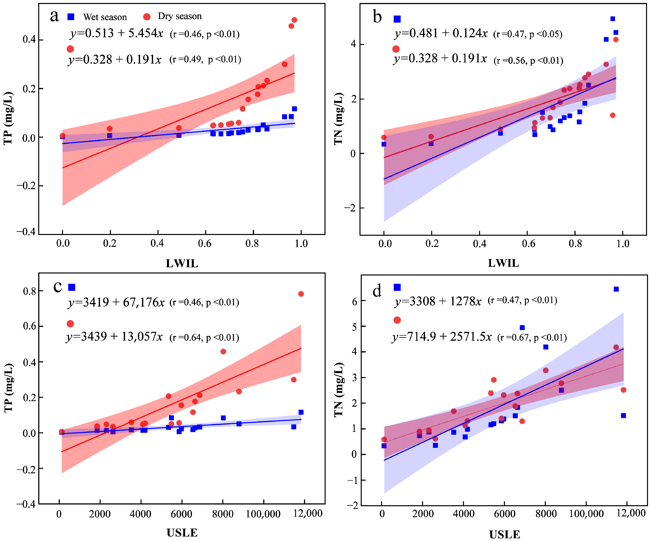
4.2. Influence of CSA Key Factors on TP and TN in the Basin

In the Caohai Lake basin, both natural and anthropogenic land use changes have significantly altered landscape patterns. When the spatial distribution of “source” and “sink” landscapes becomes imbalanced, increased N and P inputs exceed the self-purification capacity of water bodies, thereby exacerbating water quality deterioration and triggering sudden shifts in water quality [49]. Even relatively small environmental changes can lead to rapid and dramatic alterations in aquatic ecosystems [50]. The impacts of this imbalance are particularly pronounced for CSA key factors such as the LWLI and USLE. This study revealed a strong correlation between CSA factors and TN and TP concentrations. During the wet season, the LWLI and USLE collectively explained approximately 47% of the variability in TN and TP levels, while their explanatory power significantly increased to 67% during the dry season. This is likely due to the lower vegetation coverage and reduced rainfall in karst regions during the dry season, which stabilizes soil nutrients and facilitates their dissolution and transport via runoff into rivers. Consequently, CSA key factors have a more pronounced influence on water quality changes during the dry season. In contrast, nutrient transport during the wet season is more sensitive to hydrological conditions, with increased rainfall leading to rapid nutrient dilution and transport at the basin outlets [51,52].

The LWLI integrates landscape types, areas, and spatial positions to identify thresholds for sudden changes in water quality. Using non-parametric methods, frequency histograms and cumulative distribution curves were generated to explore these thresholds. The results indicated a critical breakpoint at LWLI values of around 0.75, where the cumulative probability of water quality shifts in TN and TP exceeded 60%. This suggests that beyond this threshold, the nutrient output capacity of “source” landscapes overwhelms the interception and absorption capacity of “sink” landscapes, leading to significant nutrient loss and elevated concentrations of TP and TN in water bodies. However, relying solely on landscape type, area, and spatial position may only partially explain the spatial distribution of “source” and “sink” landscapes. To address this limitation, this study further integrated the USLE with the LWLI for spatial overlay analysis, enhancing the identification of NPS pollution risks. The USLE, as a key indicator of soil erosion and nutrient loss, accounted for 56% of TN variability and 49% of TP variability. The high soil erosion risk in karst regions contributes to the transport of sediment-laden soil into rivers, intensifying the concentrations of TP and TN and influencing pollutant migration [53].

Among the USLE factors, rainfall plays a decisive role in the formation and transport of NPS pollution. During periods of heavy rainfall, increased runoff significantly amplifies pollutant transport risks. Moreover, vegetation cover has long been recognized as a critical indicator of basin health in agricultural landscapes. In karst regions, vegetation intercepts and delays rainfall infiltration into basins through permeable surfaces, thereby regulating N and P outputs during ecological succession [54,55,56]. Studies have shown that “source–sink” landscape classification effectively captures the ecological role of surface cover in nutrient loss processes. When combined with specific geological contexts, this classification better reflects the influence of surface landscape structures on P loss compared to single-factor models [57].

4.3. Management Recommendations for Non-Point Source Pollution in the Karst Caohai Lake Basin

N and P are critical indicators of watershed water quality and serve as key factors influencing landscape pattern changes. They play a significant role in optimizing the “source–sink” landscape pattern [58,59]. This study systematically investigated the spatial distribution characteristics of the landscape LWLI in the Caohai Lake basin by analyzing the migration patterns of N and P in the landscape and calculating the LWLI. In combination with the monitoring data for total TP and TN, breakpoint analyses were conducted. The results indicate that the LWLI has a significant critical effect on water quality. When the LWLI approaches 0.75, the cumulative probability of the TP and TN concentrations exceeding 60% increases substantially. Thus, optimizing the “source–sink” landscape pattern to maintain an LWLI value below 0.75 is crucial for mitigating NPS pollution risks and improving water quality [60]. However, the unique environmental and ecological characteristics of the karst region in southwestern China make land use changes significantly impactful on regional ecosystems. Due to thin soil layers, low ecological productivity, and rapid population growth, the conflict between human activities and land resources is particularly acute [61]. Simply increasing sink landscapes, such as forested and grassland areas, to reduce NPS pollution is impractical in this context [62]. Therefore, it is essential to delineate NPS pollution risk areas based on local conditions and to avoid “one-size-fits-all” management approaches. To achieve more targeted management strategies, this study integrated land use characteristics, the USLE, and the LWLI to refine the classification of potential NPS pollution risk areas in the Caohai Lake basin and proposed differentiated management recommendations.

High-risk and extremely high-risk areas are characterized by farmland proportions as high as 60–75%, indicating that farmland is the primary source of NPS pollution. When farmland area exceeds certain thresholds, the likelihood of water quality deterioration significantly increases. Optimizing farmland management is, therefore, a core measure for reducing NPS pollution. From a policy perspective, intensifying agriculture has become a key trend in rural development in southwestern China. Rational agricultural management, optimized fertilization strategies, and reduced fertilizer use can effectively minimize nutrient losses. Additionally, measures such as soil amendment using lanthanum-modified bentonite (LaMB) can further reduce N and P losses from agricultural runoff [63,64]. These approaches contribute to the lowering of the overall landscape spatial load in high-risk areas and to the improvement of soil and water quality.

Medium-risk areas are primarily affected by urban pollution sources, with urban land accounting for approximately 45%. The tributaries of Caohai Lake flow through multiple urban regions, making them more susceptible to contamination from domestic sewage. To mitigate direct pollutant entry into these tributaries, centralized sewage treatment facilities should be installed at critical nodes in urban regions. These measures can purify tributary water and reduce the impact of domestic sewage on the main basin’s water quality. Low-risk areas, influenced by karst topography, are highly sensitive to land use changes. These regions should prioritize maintaining ecosystem stability and minimizing the soil erosion caused by human activities. Additionally, increasing vegetation cover can effectively reduce soil erosion and mitigate rock desertification, thereby enhancing the resilience and sustainability of karst mountain ecosystems [65,66].

Although the “source–sink” landscape index combined with the USLE model effectively quantifies the impact of NPS pollution at the watershed scale, future studies should focus on exploring the relationship between landscape pattern evolution and pollution control. Optimizing landscape patterns in karst regions could provide a harmonized development framework for the watershed, offering scientific guidance for policymakers in implementing soil conservation measures and ecological restoration projects to promote sustainable watershed management.

5. Conclusions

This study proposed a novel method for assessing NPS pollution in karst basins using the source–sink landscape framework. CSAs were identified by integrating the landscape LWLI with the USLE model, providing scientific guidance for NPS pollution control in karst regions. The Caohai Lake basin exhibited high LWLI values, with source landscapes covering 65% of the total area. During the dry season, the LWLI explained 50–67% of the variance in TN and TP concentrations, demonstrating a strong coupling between water quality and landscape load. When the LWLI values exceeded 0.75, the TP and TN concentrations showed significant increases, with cumulative probabilities surpassing 60%, indicating heightened water quality risks. The extremely high-risk areas were primarily located in the southern and northwestern regions, where cropland and residential areas dominated. Cropland, as the primary source landscape, accounted for 75% and 60% of the extremely high-risk and high-risk zones, respectively. These areas experience severe soil erosion and high LWLI values, making them the primary sources of NPS pollution. Therefore, the management of high-risk areas should focus on optimizing farmland practices, including promoting intensive agriculture and improving soil quality to reduce nutrient losses. Additionally, vegetative buffer strips should be established at critical points within small basins to minimize the risk of pollutants entering water bodies. For medium-risk areas, management efforts should target sewage treatment in urban tributaries, with the installation of wastewater treatment facilities at key nodes to address pollution sources effectively. In low-risk areas, maintaining ecosystem stability is essential, including reducing the soil erosion caused by human activities and increasing vegetation cover to enhance the resilience and sustainability of the ecosystem.

Future research should further explore the coupling mechanisms between landscape pattern evolution and pollution control, aiming to optimize landscape patterns in karst basins. This would provide scientific support for the harmonization of ecological protection with regional development.

References

1. Varekar, V.; Yadav, V.; Karmakar, S. Rationalization of water quality monitoring locations under spatiotemporal heterogeneity of diffuse pollution using seasonal export coefficient. J. Environ. Manag. 2021, 277, 111342. [Google Scholar] [CrossRef]
2. Zou, L.; Liu, Y.; Wang, Y.; Hu, X. Assessment and analysis of agricultural non-point source pollution loads in China: 1978–2017. J. Environ. Manag. 2020, 263, 110400. [Google Scholar] [CrossRef] [PubMed]
3. Wang, Y.; Liang, J.; Yang, J.; Ma, X.; Li, X.; Wu, J.; Yang, G.; Ren, G.; Feng, Y. Analysis of the environmental behavior of farmers for non-point source pollution control and management: An integration of the theory of planned behavior and the protection motivation theory. J. Environ. Manag. 2019, 237, 15–23. [Google Scholar] [CrossRef]
4. Villamizar, M.L.; Brown, C.D. Modelling triazines in the valley of the River Cauca, Colombia, using the annualized agricultural non-point source pollution model. Agric. Water Manag. 2016, 177, 24–36. [Google Scholar] [CrossRef]
5. Shen, Z.; Qiu, J.; Hong, Q.; Chen, L. Simulation of spatial and temporal distributions of non-point source pollution load in the Three Gorges Reservoir Region. Sci. Total Environ. 2014, 493, 138–146. [Google Scholar] [CrossRef] [PubMed]
6. Zhu, X.; Li, H.; Li, Y.; Luo, Y.; Zhang, J.; Li, R. Mitigating Emerging Contaminants from Urban Non-Point Source Pollution: The Key to Achieving the SDGs. ACS ES T Water 2024, 4, 3115–3118. [Google Scholar] [CrossRef]
7. Brown, T.C.; Froemke, P. Nationwide Assessment of Nonpoint Source Threats to Water Quality. Bioscience 2012, 62, 136–146. [Google Scholar] [CrossRef]
8. Volk, M.; Liersch, S.; Schmidt, G. Towards the implementation of the European Water Framework Directive?: Lessons learned from water quality simulations in an agricultural watershed. Land Use Policy 2009, 26, 580–588. [Google Scholar] [CrossRef]
9. Xu, H.; Tan, X.; Liang, J.; Cui, Y.; Gao, Q. Impact of Agricultural Non-Point Source Pollution on River Water Quality: Evidence From China. Front. Ecol. Evol. 2022, 10, 858822. [Google Scholar] [CrossRef]
10. Alvarez, S.; Asci, S.; Vorotnikova, E. Valuing the Potential Benefits of Water Quality Improvements in Watersheds Affected by Non-Point Source Pollution. Water 2016, 8, 112. [Google Scholar] [CrossRef]
11. Rosendorf, P.; Vyskoc, P.; Prchalova, H.; Fiala, D. Estimated Contribution of Selected Non-point Pollution Sources to the Phosphorus and Nitrogen Loads in Water Bodies of the Vltava River Basin. Soil Water Res. 2016, 11, 196–204. [Google Scholar] [CrossRef]
12. Wen, W.; Zhuang, Y.; Jiang, T.; Li, W.; Li, H.; Cai, W.; Xu, D.; Zhang, L. “Period-area-source” hierarchical management for agricultural non-point source pollution in typical watershed with integrated planting and breeding. J. Hydrol. 2024, 635, 131198. [Google Scholar] [CrossRef]
13. Chen, Y.; Xu, C.-Y.; Chen, X.; Xu, Y.; Yin, Y.; Gao, L.; Liu, M. Uncertainty in simulation of land-use change impacts on catchment runoff with multi-timescales based on the comparison of the HSPF and SWAT models. J. Hydrol. 2019, 573, 486–500. [Google Scholar] [CrossRef]
14. Volk, M.; Bosch, D.; Nangia, V.; Narasimhan, B. SWAT: Agricultural water and Nonpoint source pollution management at a watershed scale. Agric. Water Manag. 2016, 175, 1–3. [Google Scholar] [CrossRef]
15. Guo, J.; Wang, Y.; Lai, J.; Pan, C.; Wang, S.; Fu, H.; Zhang, B.; Cui, Y.; Zhang, L. Spatiotemporal distribution of nitrogen biogeochemical processes in the coastal regions of northern Beibu Gulf, south China sea. Chemosphere 2020, 239, 124803. [Google Scholar] [CrossRef] [PubMed]
16. Wang, R.; Wang, Y.; Sun, S.; Cai, C.; Zhang, J. Discussing on “source-sink” landscape theory and phytoremediation for non-point source pollution control in China. Environ. Sci. Pollut. Res. 2020, 27, 44797–44806. [Google Scholar] [CrossRef] [PubMed]
17. Zhao, C.; Li, M.; Wang, X.; Liu, B.; Pan, X.; Fang, H. Improving the accuracy of nonpoint-source pollution estimates in inland waters with coupled satellite-UAV data. Water Res. 2022, 225, 119208. [Google Scholar] [CrossRef] [PubMed]
18. Jia, X.; Fu, T.; Hu, B.; Shi, Z.; Zhou, L.; Zhu, Y. Identification of the potential risk areas for soil heavy metal pollution based on the source-sink theory. J. Hazard. Mater. 2020, 393, 122424. [Google Scholar] [CrossRef]
19. Brinkmann, R.; Parise, M. Karst environments: Problems, management, human impacts, and sustainability an introduction to the special issue. J. Cave Karst Stud. 2012, 74, 135–136. [Google Scholar] [CrossRef]
20. Li, S.; Liu, C.; Chen, J.; Wang, S. Karst ecosystem and environment: Characteristics, evolution processes, and sustainable development. Agric. Ecosyst. Environ. 2021, 306, 107173. [Google Scholar] [CrossRef]
21. Li, S.; Xu, S.; Wang, T.; Yue, F.; Peng, T.; Zhong, J.; Wang, L.; Chen, J.; Wang, S.; Chen, X.; et al. Effects of agricultural activities coupled with karst structures on riverine biogeochemical cycles and environmental quality in the karst region. Agric. Ecosyst. Environ. 2020, 303, 107120. [Google Scholar] [CrossRef]
22. Wang, Z.; Liu, C.; Qiao, G. Effect of Nitrogen and Phosphorus Cycling Characteristic on Eutrophication of Water Body. South-to-North Water Transf. Water Sci. Technol. 2010, 8, 82–85, 97. [Google Scholar] [CrossRef]
23. Elser, J.J.; Bracken ME, S.; Cleland, E.E.; Gruner, D.S.; Harpole, W.S.; Hillebrand, H.; Ngai, J.T.; Seabloom, E.W.; Shurin, J.B.; Smith, J.E. Global analysis of nitrogen and phosphorus limitation of primary producers in freshwater, marine and terrestrial ecosystems. Ecol. Lett. 2007, 10, 1135–1142. [Google Scholar] [CrossRef] [PubMed]
24. Chen, X.; Lv, L.; He, C. Study on the causes and countermeasures of water pollution and water environment problems in the Caohai sub-watershed of Weining, Guizhou Province. Groundwater 2022, 44, 83–85. (In Chinese) [Google Scholar]
25. Zhou, Q.; Tong, D.; Zhang, H. Analysis of the ecological status and control measures of Caohai. Soil Water Conserv. China 2018, 3, 59–61. (In Chinese) [Google Scholar]
26. Chen, L.D.; Fu, B.J.; Zhao, W. Source-sink landscape theory and its ecological significance. Front. Biol. China 2008, 3, 1444–1449. [Google Scholar] [CrossRef]
27. Wang, G.; Li, J.; Sun, W.; Xue, B.; Yinglan, A.; Liu, T. Non-point source pollution risks in a drinking water protection zone based on remote sensing data embedded within a nutrient budget model. Water Res. 2019, 157, 238–246. [Google Scholar] [CrossRef] [PubMed]
28. Cui, M.; Guo, Q.; Wei, R.; Wei, Y. Anthropogenic nitrogen and phosphorus inputs in a new perspective: Environmental loads from the mega economic zone and city clusters. J. Clean. Prod. 2021, 283, 124589. [Google Scholar] [CrossRef]
29. Lu, C.; Zhang, H.; Qi, L. Critical Source Area Identification and Risk Assessment of Agricultural Non-Point Source Pollution of the Source Areas of Liaohe River Watershed. Acta Agric. Univ. Jiangxiensis 2014, 36, 670–677. [Google Scholar]
30. Karra, K.; Kontgis, C.; Weil, Z.S.; Mazzariello, M.M.; Steven, P.M.; Brumby, S.P. Global land use/land cover with Sentinel-2 and deep learning. In Proceedings of the IEEE International Geoscience and Remote Sensing Symposium IGARSS, Brussels, Belgium, 11–16 July 2021; pp. 4704–4707. [Google Scholar]
31. Cai, C.; Ding, S.; Shi, Z.; Huang, L.; Zhang, G. Study on the prediction of soil erosion in small watersheds using the USLE model and GIS IDRISI. J. Soil Water Conserv. 2000, 14, 19–24. (In Chinese) [Google Scholar]
32. King, R.S.; Richardson, C.J. Integrating Bioassessment and Ecological Risk Assessment: An Approach to Developing Numerical Water-Quality Criteria. Environ. Manag. 2003, 31, 795–809. [Google Scholar] [CrossRef]
33. Qian, S.S.; King, R.S.; Richardson, C.J. Two statistical methods for the detection of environmental thresholds. Ecol. Model. 2003, 166, 87–97. [Google Scholar] [CrossRef]
34. Wang, J.; Qiu, C.; Qin, S.; Yao, S.; Chen, J.; Lei, S.; Tan, S.; Zhou, B. Effects of “source-sink” landscape on spatiotemporal differentiation of phosphorus output in multiple watersheds in mountainous areas based on the modified location-weighted landscape index. Ecol. Indic. 2024, 158, 111397. [Google Scholar] [CrossRef]
35. Narany, T.S.; Aris, A.Z.; Sefie, A.; Keesstra, S. Detecting and predicting the impact of land use changes on groundwater quality, a case study in Northern Kelantan, Malaysia. Sci. Total Environ. 2017, 599, 844–853. [Google Scholar] [CrossRef] [PubMed]
36. Ahearn, D.S.; Sheibley, R.W.; Dahlgren, R.A.; Anderson, M.; Johnson, J.; Tate, K.W. Land use and land cover influence on water quality in the last free-flowing river draining the western Sierra Nevada, California. J. Hydrol. 2005, 313, 234–247. [Google Scholar] [CrossRef]
37. Chen, L.; Sun, R.; Lu, Y. A conceptual model for a process-oriented landscape pattern analysis. Sci. China-Earth Sci. 2019, 62, 2050–2057. [Google Scholar] [CrossRef]
38. Pi, X.; Luo, Q.; Feng, L.; Xu, Y.; Tang, J.; Liang, X.; Ma, E.; Cheng, R.; Fensholt, R.; Brandt, M.; et al. Mapping global lake dynamics reveals the emerging roles of small lakes. Nat. Commun. 2022, 13, 5777. [Google Scholar] [CrossRef]
39. Williamson, C.E.; Saros, J.E.; Vincent, W.F.; Smol, J.P. Lakes and reservoirs as sentinels, integrators, and regulators of climate change. Limnol. Oceanogr. 2009, 54, 2273–2282. [Google Scholar] [CrossRef]
40. Ou, Y.; Rousseau, A.N.; Yan, B.; Zhang, Y.; Sui, Y.; Cui, H. Identifying the critical lakeshore zone to optimize landscape factors for improved lake water quality in a semi-arid region of Northeastern China. Ecol. Indic. 2023, 154, 110834. [Google Scholar] [CrossRef]
41. Hu, N.; Tang, Q.; Sheng, Y. Effect of salinity on the determination of dissolved non-reactive phosphorus and total dissolved phosphorus in coastal waters. Water Environ. Res. 2022, 94, e10706. [Google Scholar] [CrossRef]
42. Shah, N.W.; Baillie, B.R.; Bishop, K.; Ferraz, S.; Hogbom, L.; Nettles, J. The effects of forest management on water quality. For. Ecol. Manag. 2022, 522, 120397. [Google Scholar] [CrossRef]
43. Trogisch, S.; Liu, X.; Rutten, G.; Xue, K.; Bauhus, J.; Brose, U.; Bu, W.; Cesarz, S.; Chesters, D.; Connolly, J.; et al. The significance of tree-tree interactions for forest ecosystem functioning. Basic Appl. Ecol. 2021, 55, 33–52. [Google Scholar] [CrossRef]
44. Duffy, C.; O’Donoghue, C.; Ryan, M.; Kilcline, K.; Upton, V.; Spillane, C. The impact of forestry as a land use on water quality outcomes: An integrated analysis. For. Policy Econ. 2020, 116, 102185. [Google Scholar] [CrossRef]
45. Johnston, C.A.; Bubenzer, G.D.; Lee, G.B.; Madison, F.W.; McHenry, J.R. Nutrient trapping by sediment deposition in a seasonally flooded lakeside wetland. J. Environ. Qual. 1984, 13, 283–290. [Google Scholar] [CrossRef]
46. Wang, L.; Dalabay, N.; Lu, P.; Wu, F. Effects of tillage practices and slope on runoff and erosion of soil from the Loess Plateau, China, subjected to simulated rainfall. Soil Tillage Res. 2017, 166, 147–156. [Google Scholar] [CrossRef]
47. Ribeiro Correa, T.L.; de Queiroz, M.V.; de Araujo, E.F. Cloning, recombinant expression and characterization of a new phytase from Penicillium chrysogenum. Microbiol. Res. 2015, 170, 205–212. [Google Scholar] [CrossRef] [PubMed]
48. Yin, C.; Yang, H.; Wang, J.; Guo, J.; Tang, X.; Chen, J. Combined use of stable nitrogen and oxygen isotopes to constrain the nitrate sources in a karst lake. Agric. Ecosyst. Environ. 2020, 303, 107089. [Google Scholar] [CrossRef]
49. Vrebos, D.; Beauchard, O.; Meire, P. The impact of land use and spatial mediated processes on the water quality in a river system. Sci. Total Environ. 2017, 601, 365–373. [Google Scholar] [CrossRef]
50. Ficetola, G.F.; Denoel, M. Ecological thresholds: An assessment of methods to identify abrupt changes in species-habitat relationships. Ecography 2009, 32, 1075–1084. [Google Scholar] [CrossRef]
51. Yu, W.; Zhang, J.; Liu, L.; Li, Y.; Li, X. A source-sink landscape approach to mitigation of agricultural non-point source pollution: Validation and application. Environ. Pollut. 2022, 314, 120287. [Google Scholar] [CrossRef] [PubMed]
52. Wu, Z.; Lai, X.; Li, K. Water quality assessment of rivers in Lake Chaohu Basin (China) using water quality index. Ecol. Indic. 2021, 121, 107021. [Google Scholar] [CrossRef]
53. Li, Q.; Liu, G.-B.; Zhang, Z.; Tuo, D.-F.; Bai, R.-R.; Qiao, F.-F. Relative contribution of root physical enlacing and biochemistrical exudates to soil erosion resistance in the Loess soil. Catena 2017, 153, 61–65. [Google Scholar] [CrossRef]
54. Salhi, A.; Benabdelouahab, S.; Bouayad, E.O.; Benabdelouahab, T.; Larifi, I.; El Mousaoui, M.; Acharrat, N.; Himi, M.; Ponsati, A.C. Impacts and social implications of landuse-environment conflicts in a typical Mediterranean watershed. Sci. Total Environ. 2021, 764, 142853. [Google Scholar] [CrossRef]
55. Zhao, S.; Pereira, P.; Wu, X.; Zhou, J.; Cao, J.; Zhang, W. Global karst vegetation regime and its response to climate change and human activities. Ecol. Indic. 2020, 113, 106208. [Google Scholar] [CrossRef]
56. De Paula, F.R.; Gerhard, P.; de Barros Ferraz, S.F.; Wenger, S.J. Multi-scale assessment of forest cover in an agricultural landscape of Southeastern Brazil: Implications for management and conservation of stream habitat and water quality. Ecol. Indic. 2018, 85, 1181–1191. [Google Scholar] [CrossRef]
57. Wang, J.; Ni, J.P.; Chen, C.L.; Xie, D.T.; Shao, J.A.; Chen, F.X.; Lei, P. Source-sink landscape spatial characteristics and effect on non-point source pollution in a small catchment of the Three Gorge Reservoir Region. J. Mt. Sci. 2018, 15, 327–339. [Google Scholar] [CrossRef]
58. Wu, J.; Lu, J. Landscape patterns regulate non-point source nutrient pollution in an agricultural watershed. Sci. Total Environ. 2019, 669, 377–388. [Google Scholar] [CrossRef] [PubMed]
59. Xu, M.; Xu, G.; Li, Z.; Dang, Y.; Li, Q.; Min, Z.; Gu, F.; Wang, B.; Liu, S.; Zhang, Y. Effects of comprehensive landscape patterns on water quality and identification of key metrics thresholds causing its abrupt changes. Environ. Pollut. 2023, 333, 122097. [Google Scholar] [CrossRef] [PubMed]
60. Qiu, J.; Turner, M.G. Importance of landscape heterogeneity in sustaining hydrologic ecosystem services in an agricultural watershed. Ecosphere 2015, 6, 1–19. [Google Scholar] [CrossRef]
61. Liu, C.Q. Biogeochemical Processes and Matter Cycle of the Earth’s Surface—The Basin Weathering of South-West Karst Area and Nutrients Elements Cycle; Science Press: Beijing, China, 2009; pp. 169–192. [Google Scholar]
62. Zhang, K.-M.; Wen, Z.-G. Review and challenges of policies of environmental protection and sustainable development in China. J. Environ. Manag. 2008, 88, 1249–1261. [Google Scholar] [CrossRef] [PubMed]
63. Juncal MJ, L.; Masino, P.; Bertone, E.; Stewart, R.A. Towards nutrient neutrality: A review of agricultural runoff mitigation strategies and the development of a decision-making framework. Sci. Total Environ. 2023, 874, 162408. [Google Scholar] [CrossRef]
64. Wang, J.; Chen, J.; Jin, Z.; Guo, J.; Yang, H.; Zeng, Y.; Liu, Y. Simultaneous removal of phosphate and ammonium nitrogen from agricultural runoff by amending soil in lakeside zone of Karst area, Southern China. Agric. Ecosyst. Environ. 2020, 289, 106745. [Google Scholar] [CrossRef]
65. Hu, Z.; Wang, S.; Bai, X.; Luo, G.; Li, Q.; Wu, L.; Yang, Y.; Tian, S.; Li, C.; Deng, Y. Changes in ecosystem service values in karst areas of China. Agric. Ecosyst. Environ. 2020, 301, 107026. [Google Scholar] [CrossRef]
66. Tong, X.; Brandt, M.; Yue, Y.; Ciais, P.; Rudbeck Jepsen, M.; Penuelas, J.; Wigneron, J.P.; Xiao, X.; Song, X.P.; Horion, S.; et al. Forest management in southern China generates short term extensive carbon sequestration. Nat. Commun. 2020, 11, 129. [Google Scholar] [CrossRef]
67. Zhang, Y.; Li, Z.; Wang, T.; Wang, P.; Xu, R.; Wang, J. Effects of source-sink landscape proximity on the spatial-temporal water quality from the perspective of cost distance in an agricultural basin. J. Hydrol. 2024, 628, 130569. [Google Scholar] [CrossRef]
68. Liu, L.; Zhong, Q.; Ni, J. Ecological stoichiometry characteristics and storage of C, N, and P in secondary forests of the karst region on the Guizhou Plateau. Acta Ecol. Sin. 2019, 39, 8606–8614. (In Chinese) [Google Scholar]
69. Ma, X.; Li, Y.; Zhang, M.; Zheng, F.; Du, S. Assessment and analysis of non-point source nitrogen and phosphorus loads in the Three Gorges Reservoir Area of Hubei Province, China. Sci. Total Environ. 2011, 412, 154–161. [Google Scholar] [CrossRef] [PubMed]
70. Zhan, S.; Chen, F.; Hu, X. Availability of soil nitrogen and phosphorus at typical stages of forest succession in the hilly red soil region of the central subtropics. Acta Ecol. Sin. 2009, 29, 4673–4680. (In Chinese) [Google Scholar]
71. Skinner, M. Wetland phosphorus dynamics and phosphorus removal potential. Water Environ. Res. 2022, 94, e10799. [Google Scholar] [CrossRef]
72. Walton, C.R.; Zak, D.; Audet, J.; Petersen, R.J.; Lange, J.; Oehmke, C.; Wichtmann, W.; Kreyling, J.; Grygoruk, M.; Jablonska, E.; et al. Wetland buffer zones for nitrogen and phosphorus retention: Impacts of soil type, hydrology and vegetation. Sci. Total Environ. 2020, 727, 138709. [Google Scholar] [CrossRef] [PubMed]
Figure 1. Study area overview. (a) Geographical location of Guizhou in China. (b) Land use distribution of the Caohai Lake basin. This map illustrates the major land use types within the study area, including cropland, forest, grassland, wetland, lake, residential land areas, and bare land. Different colors represent various land use categories. (c) Sub-basin divisions and hydrological network of the Caohai basin, where the blue areas represent lakes, the red points mark the water quality monitoring stations, and the black lines denote the boundaries of sub-basins, with numbers serving to identify each sub-basin. Major rivers, including the Dazhong River, Dongshan River, Baima River, Maojiahai River, and Wanxia River, radiate through the basin and converge into Caohai Lake.
Water 17 00132 g001
Figure 2. Spatial distribution of landscape load indices. (a) TN landscape load index: gradient shading from light to dark represents areas with increasing TN load levels. (b) TP landscape load index: gradient shading from light to dark illustrates variations in TP load levels. (c) Integrated landscape load index in the Caohai Lake basin: combines TN and TP load distributions, with darker colors indicating higher landscape loads and greater pollution potential.
Water 17 00132 g002
Figure 3. LWLI threshold analysis. The x-axis represents the landscape LWLI, indicating the impact of varying load levels on basin pollution. The left y-axis shows the frequency count, representing the number of sampling points within each LWLI range. The right y-axis depicts the cumulative threshold frequency, illustrating the trend in cumulative sampling point frequencies as LWLI values increase. The red dashed line represents the LWLI threshold, indicating the critical value where significant changes in TN or TP pollution levels are observed.
Water 17 00132 g003
Figure 4. Map of critical source areas for non-point source pollution. Spatial distribution of land use types (a). Soil erosion modulus (b). Division of critical source areas in Caohai Lake Basin (c). The colors represent different pollution risk zones, including low-risk, medium-risk, high-risk, and extremely high-risk areas. This operation was completed through weighted overlay in ArcMap 10.7, with the weights of land use, soil erosion, and LWLI being 0.2, 0.4, and 0.4, respectively.
Water 17 00132 g004
Figure 5. Proportion of landscape types across different risk areas. The bar chart illustrates the cumulative area, with different colors representing various landscape types, namely grasslands, residential areas, bare land, cropland, forests, wetlands, and lakes.
Water 17 00132 g005
Figure 6. Heatmap of correlations between watershed water quality and CSA key factors, where the color of the matrix represents the Pearson correlation coefficient (r value) between the parameters, with darker colors indicating stronger correlations. The color bar on the right shows the gradient from negative to positive correlations. Colors range from red (negative correlation) to green (positive correlation), and the color and thickness of lines connecting the source to sink landscapes indicate the results of the Mantel test, with red lines representing significant positive correlations, blue lines representing negative correlations, and line thickness indicating the strength of the correlation.
Water 17 00132 g006
Figure 7. Regression analysis of CSA with TP and TN. (a,b): Regression analysis of LWLI with TP (a) and TN (b) during wet (blue) and dry (red) seasons. (c,d): Regression analysis of USLE with TP (c) and TN (d) during wet (blue) and dry (red) seasons. Shaded areas represent 95% confidence intervals, illustrating seasonal differences in the relationships between LWLI, USLE, and nutrient concentrations.
Water 17 00132 g007