Article

Daily Streamflow Forecasting Using Networks of Real-Time Monitoring Stations and Hybrid Machine Learning Methods

1
School of Engineering, University of Guelph, 50 Stone Road East, Guelph, ON N1G 2W1, Canada
2
Lakes Environmental, 170 Columbia St. W, Waterloo, ON N2L 3L3, Canada
*
Authors to whom correspondence should be addressed.
Water 2024, 16(9), 1284; https://doi.org/10.3390/w16091284
Submission received: 10 March 2024 / Revised: 26 April 2024 / Accepted: 26 April 2024 / Published: 30 April 2024

Abstract

:
Considering the increased risk of urban flooding and drought due to global climate change and rapid urbanization, the imperative for more accurate methods for streamflow forecasting has intensified. This study introduces a pioneering approach leveraging the available network of real-time monitoring stations and advanced machine learning algorithms that can accurately simulate spatial–temporal problems. The Spatio-Temporal Attention Gated Recurrent Unit (STA-GRU) model is renowned for its computational efficacy in forecasting streamflow events with a forecast horizon of 7 days. The novel integration of the groundwater level, precipitation, and river discharge as predictive variables offers a holistic view of the hydrological cycle, enhancing the model’s accuracy. Our findings reveal that for a 7-day forecasting period, the STA-GRU model demonstrates superior performance, with a notable improvement in mean absolute percentage error (MAPE) values and R-square ( R 2 ) alongside reductions in the root mean squared error (RMSE) and mean absolute error (MAE) metrics, underscoring the model’s generalizability and reliability. Comparative analysis with seven conventional deep learning models, including the Long Short-Term Memory (LSTM), the Convolutional Neural Network LSTM (CNNLSTM), the Convolutional LSTM (ConvLSTM), the Spatio-Temporal Attention LSTM (STA-LSTM), the Gated Recurrent Unit (GRU), the Convolutional Neural Network GRU (CNNGRU), and the STA-GRU, confirms the superior predictive power of the STA-LSTM and STA-GRU models when faced with long-term prediction. This research marks a significant shift towards an integrated network of real-time monitoring stations with advanced deep-learning algorithms for streamflow forecasting, emphasizing the importance of spatially and temporally encompassing streamflow variability within an urban watershed’s stream network.

1. Introduction

Hydrological forecasting involves predicting streamflow, rainfall–runoff, and other hydrological variables, which are vital for water resource management, environmental planning, and addressing hydrological extremes such as floods, droughts, and variations in streamflow [1,2,3]. In the context of streamflow forecasting, the utilization of groundwater level data has become increasingly significant, underpinned by the hydrological principle of the interaction between groundwater and surface water. The variation in groundwater levels not only reflects the recharge of groundwater resources following precipitation infiltration but also indicates the contribution of groundwater to river flow, especially in predicting and mitigating drought impacts [4,5].
Understanding the relationship between groundwater levels and streamflow is critical for effective water resource management and proper preparation for drought conditions [6,7,8]. The fluctuations in groundwater levels play a pivotal role in influencing soil moisture availability, directly impacting the occurrence and duration of soil drought conditions [9,10,11]. During drought periods, groundwater is a critical source of moisture through capillary action, supporting plant growth and maintaining soil hydration [12,13]. However, a persistent decline in groundwater levels disrupts this replenishment mechanism, gradually depleting soil moisture storage and exacerbating soil drought severity.
Moreover, lowering groundwater levels can also lead to the upward migration of soil salts, exacerbating soil salinization issues, which negatively affect vegetation cover and agricultural productivity [14,15,16]. Therefore, monitoring and modeling groundwater levels are crucial in developing effective drought early warning systems and response strategies. A deeper understanding of groundwater and soil moisture dynamics enables more accurate predictions of drought likelihood and severity, providing a scientific basis for water resource management and agricultural irrigation planning.
The advancement of remote sensing technology and Geographic Information Systems (GIS) has made monitoring and predicting groundwater levels more precise and efficient [17,18,19]. Data fusion techniques allow for integrating groundwater level monitoring data with other hydro-meteorological data, providing more comprehensive and accurate data support for streamflow forecasting.
Despite the potential value of groundwater level data in streamflow forecasting, their application has challenges and limitations [20]. For instance, the acquisition of groundwater level data may be constrained by the density of monitoring networks and monitoring technology. Additionally, the complex interactions between groundwater dynamics and surface water require accurate simulation through advanced models [21,22,23].

1.1. Streamflow Prediction Models

The advancement of machine learning models, such as Artificial Neural Networks (ANNs), Adaptive Neuro-Fuzzy Inference Systems (ANFISs), and Support Vector Machines (SVMs), offers new opportunities for improving the accuracy of streamflow predictions [5,24,25,26,27,28,29,30]. By integrating groundwater levels with other key hydrological variables (e.g., rainfall, river water discharge, soil moisture), these models provide a more nuanced understanding of hydrological processes, enabling better management of water resources during both surplus and deficit conditions.
This part also introduces the evolution of deep learning in hydrology [31,32]. It discusses the shift from traditional models to data-driven approaches and highlights the advantages of deep learning in capturing nonlinear relationships and spatial dependencies. Early deep learning applications in hydrology, such as Long Short-Term Memory (LSTM) networks, are examined [33,34].
Since LSTM has a unique internal structure that allows it to handle and remember long-term sequential dependencies, it is an excellent option for solving these issues [27,35,36,37]. Streamflow forecasting is a classic time-series prediction issue where LSTM is promising [26,38,39]. This method necessitates managing and comprehending constant meteorological and hydrological data to anticipate future streamflows. However, most LSTM models are mainly used for rainfall and river discharge forecasting for individual sites [40].
With the development of deep learning technology, scientists started experimenting with more intricate models—such as the Generalized Structure of Group Method of Data Handling (GSGMDH) and combinations of Convolutional Neural Networks (CNNs) with LSTM—to deal with meteorological and hydrological data from various geographic locations [41,42,43]. These models are helpful for streamflow prediction in multiple catchments because they successfully integrate spatial and temporal information accurately. This explains how LSTMs capture the temporal correlations between spatial patterns and how CNNs encode them. It offers case examples that show how Convolutional Neural Network LSTM (CNNLSTM) models work well to estimate daily streamflow with high accuracy [44,45].
Streamflow prediction is a data-driven challenge. It also necessitates attention to several intricate affecting elements caused by humans and nature. Hybrid models are widely used as they improve the stability and generalizability of single models. While deep learning models such as LSTM, CNNLSTM, convolutional LSTM (ConvLSTM), and others have demonstrated great promise in streamflow prediction, further refinement and optimization of these models are required to tackle the diverse obstacles associated [46,47].
Furthermore, the attention method can help the model cope with long-term dependencies more successfully since the streamflow prediction dataset comprises both time series and spatial series, with a vast amount of data over a long period. The attention mechanism can raise prediction accuracy by assisting the model in more effectively extracting relevant information from the input data. Regarding streamflow forecasting, the Spatio-Temporal Attention LSTM (STA-LSTM) model has proven effective [48].
Accuracy should be guaranteed, but prediction models should aim for maximum computing efficiency. Based on ideas from the LSTM model, the Gated Recurrent Unit (GRU) is a forecasting model [49,50,51]. Although the study findings with GRUs and LSTM are comparable, there are some significant differences between the two models. For example, GRUs have an excellent numerical ability, indicating that they can efficiently acquire and remember important information over extended periods. This capability is essential for jobs that need long-term dependencies, as the model must generate accurate predictions by considering historical data.
A gating mechanism in the GRU model allows it to update its hidden state only when necessary in response to input data. Specifically, a GRU uses an update gate, which combines the functions of input and LSTM forget gates [49,52]. This combination shortens training durations and improves computational efficiency by streamlining the architecture and lowering the number of parameters.
Additionally, the efficient information flow inside the model is promoted by the streamlined architecture of the GRU, which combines the hidden state and cell state. The GRU’s design facilitates the extraction of pertinent information and the elimination of extraneous details, making it especially appropriate for jobs that require sequential data analysis. The usefulness of the GRU and Convolutional Neural Network GRU (CNNGRU) models for streamflow prediction has been investigated throughout the last two years [53,54]. Regarding short-term streamflow projections, the GRU model outperforms the LSTM [55].
Table 1 compares different machine learning models based on their daily streamflow prediction performance, considering both models that account for spatio-temporal dynamics and those that do not. The variety of models demonstrates the breadth of approaches in the field, with each model exhibiting different strengths in prediction accuracy and error metrics. Fine-tuning pre-trained deep-learning models for regional hydrological modeling is another area of interest. By calibrating models for a broad region and then adapting them to specific catchments with limited data, researchers aim to address the challenge of data scarcity in hydrology.

1.2. Advancements in Streamflow Forecasting through Deep Learning

In employing deep learning techniques to analyze large spatio-temporal datasets, two prevalent challenges encountered are the vanishing gradient problem and overfitting [56,57,58]. These issues often result in minimal weight updates, leading to significantly slow learning rates or worse scenarios with a complete inability for the network to learn. LSTM and GRUs introduce gating mechanisms that allow the network to control the flow of information more flexibly, enabling the retention of long-term dependencies while preventing gradient vanishing during the training of long sequences, thereby effectively mitigating the vanishing gradient problem [59,60].
Moreover, the transition of datasets from an hourly to a daily granularity exacerbates these challenges, necessitating models that can swiftly identify and learn crucial features from the now more compact datasets. The attention mechanism can quickly identify and learn key features when the dataset is small [61,62].
Therefore, this paper aims to contribute to the field by introducing the STA-LSTM and STA-GRU models, which integrate a spatial–temporal attention mechanism within the conventional LSTM and GRU frameworks. This attention mechanism enhances the model’s performance on smaller datasets by enabling more focused and efficient identification and learning of critical data features. Applying spatial–temporal mechanisms within these models facilitates superior learning in spatio-temporal datasets. Furthermore, the research brings new content to the issue by integrating groundwater level data with conventional precipitation and discharge station data, thus enhancing the deep learning methodologies’ performance, especially in predicting low flow conditions.
Such advancements are particularly crucial for tasks that are reliant on temporal and spatial data dimensions, including streamflow prediction. By proposing STA-LSTM and STA-GRU models that incorporate spatial–temporal attention mechanisms, this paper addresses the deep learning challenges presented by changes in data granularity and dataset size reduction, offering novel methodologies for practical spatio-temporal data analysis.

2. Materials and Methods

Figure 1 constitutes a detailed cartographic depiction of the Credit River Watershed, which has been annotated to identify the hydrological monitoring infrastructure within the region. The map artfully delineates the stream network with comprehensive blue lines, clearly representing the fluvial pathways. A legend explains the symbology employed, while the orientation and scale are conveyed through an unambiguous north arrow and a graduated scale bar, respectively. Based on the provided map of the Credit River Watershed, the catchment area can be characterized as a region with a well-developed hydrological monitoring infrastructure. The catchment includes a network of hydrometric, climate, and groundwater level stations that collectively provide data essential for forecasting and ecological conservation efforts.
Strategically situated hydrometric monitoring stations are denoted by dark blue square signs, each bearing unique alphanumeric identifiers such as 02HB001 and 02HB031. These stations are instrumental in collecting hydrological data, playing a pivotal role in assessing aquatic resource distribution, streamflow forecasting, and ecological conservation efforts.
Additionally, the map illustrates the spatial distribution of precipitation stations (green circle signs) and groundwater level stations (pink rhombus signs), marked with labels such as P6152695 and W0000165. The role of these stations is crucial in quantifying precipitation and groundwater level inputs, serving as a foundation for hydrological modeling and the comprehensive analysis of the watershed’s hydrological cycle.
The hydrometric station 02HB029 is strategically positioned near Mississauga, which is central to the hydrological analysis. This station serves as the terminus for hydrological predictive models tasked with projecting the discharge values over a forthcoming 7 day interval. We utilized data from 14 hydrological stations spanning from 1 April 2006 to 31 March 2021. This dataset includes 7 river discharge stations, 4 groundwater level stations, and 3 precipitation stations. The 15-year historical dataset was divided for model training, validation, and testing purposes, allocating 70% for training, 10% for validation, and 20% for testing.
In Figure 2, four distinct curves corresponding to different data series—02HB029 (DC29), 02HB025 (DC25), 02HB018 (DC18), and W0000165 (GW165)—are observable. These curves indicate groundwater level and discharge measurements taken from various locations or under varying conditions. For example, all series converge to reach a peak on approximately 28 December 2008. This simultaneous peak in groundwater level (GW165) and discharge (DC29, DC25, DC18) suggests a near-instantaneous response of the groundwater to changes in river discharge. This implies that the rise in groundwater level and the increase in river discharge occur concurrently, with no significant lag time discernible.
In the predictive model, DC29 serves as the output variable and is situated at the outlet of the watershed in a heavily urbanized area. This station exhibits a slightly higher ratio of standard deviation over the mean, which is indicative of the impervious urban area’s impact on the variability and extreme flow events (flash floods) as Table 2. There is also a notable difference in the mean precipitation at station P6152695, which is likely due to an escarpment that affects the local wind patterns and precipitation.

2.1. The Correlation of Discharge, Groundwater Level, and Precipitation

The heatmap in Figure 3 is a graphical representation of the correlation coefficients between various variables; such heatmaps are commonly utilized to discern the strength and direction of linear relationships within a dataset. Correlation values are contained within the range of −1 to 1, where 1 denotes a perfect positive linear correlation, −1 denotes a perfect negative linear correlation, and 0 indicates no linear correlation. The color scheme of the heatmap, ranging from dark red to dark blue, visually emphasizes the strength of the positive and negative correlations, respectively, with lighter shades indicating weaker correlations.
In predicting outputs for streamflow station DC29, it is imperative to identify variables with substantial correlations. The variables DC25 and DC18 exhibit robust positive correlations with DC29, with coefficients of 0.98 and 0.94, respectively. This suggests that these variables are potentially significant predictors of DC29’s output.
The watershed is also subject to climate change, leading to significant temperature, precipitation, and evapotranspiration trends [63,64]. Although precipitation has shown an increasing trend, so has evapotranspiration, which could offset the potential increase in discharge that might be expected from more rainfall [65]. The increased temperature could lead to higher evaporation and plant transpiration rates, further reducing the amount of rainfall that contributes to groundwater recharge and surface water levels.
Given these factors, the low impact of rainfall on discharges in the Credit River Watershed can be attributed to the combined effects of urbanization, land use diversity, climate change, and the complex hydrological processes that govern the movement and storage of water within the watershed.
Moreover, the positive correlations among all the hydrological stations indicate that the influences between the chosen stations are consistent with natural hydrological patterns. This conformity implies that the selected stations are interrelated and can be reliably employed in subsequent hydrological prediction.
For constructing a predictive model for the downstream discharge (DC29 is located in an urban area), the selection of predictors should be executed with a nuanced understanding of the data to ensure that correlations are meaningful and not merely incidental. Moreover, it is crucial to address the issue of multicollinearity, wherein several independent variables are highly correlated, as this can undermine the reliability of the model’s coefficients. Employing advanced machine learning techniques can facilitate the integration of multiple predictive variables to establish a robust predictive model for the water station DC29’s output.
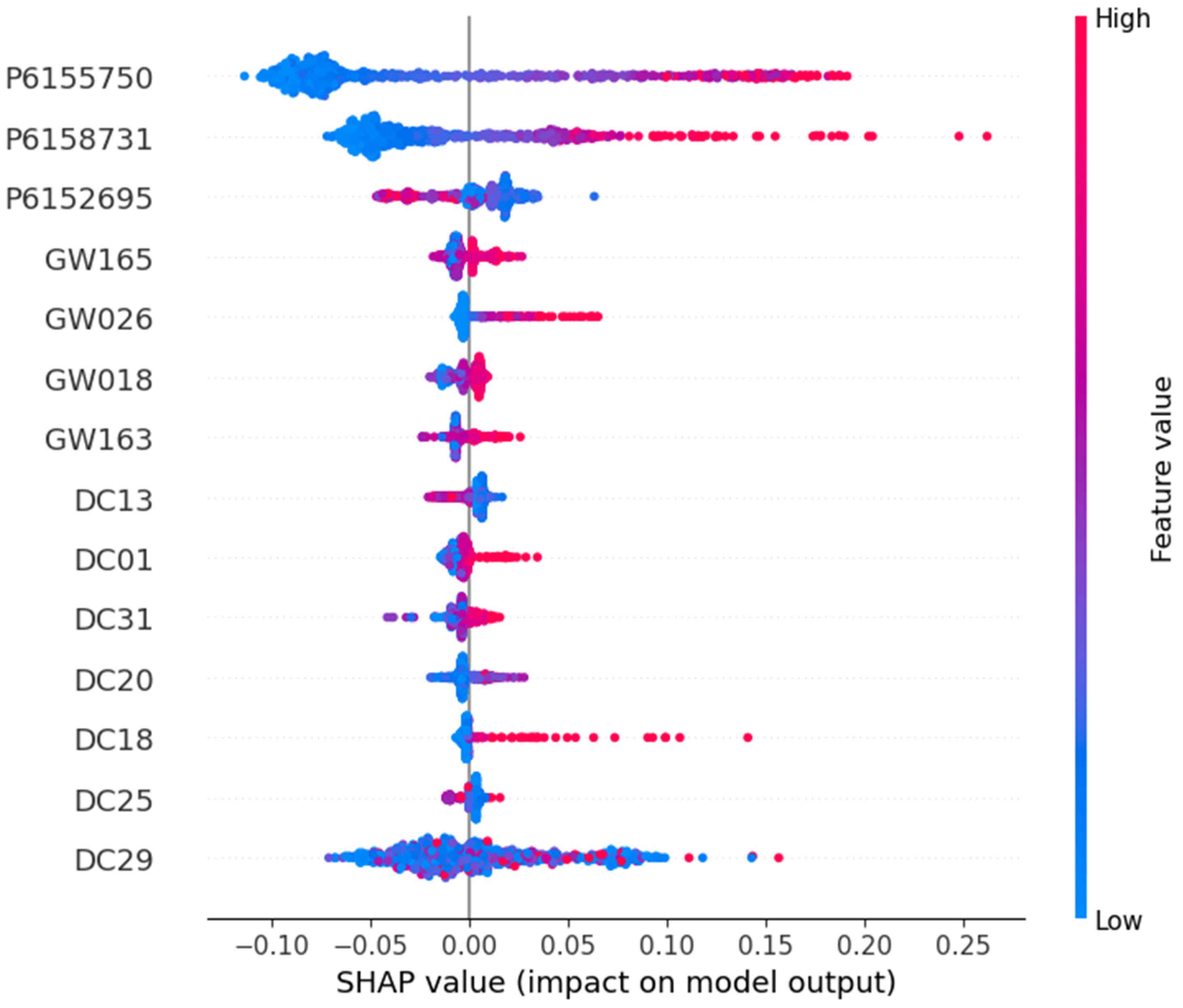
The Shapley Additive Explanations (SHAP) summary plot provides a comprehensive visualization of the feature contributions across all observations in the dataset to present their impact on the predictive model output. The TreeExplainer, a model-agnostic tool provided by the SHAP library, is used to analyze an XGBoost model trained on our dataset. Before data input, the data are processed through Min–Max Normalization. The XGBoost model is trained with a learning rate of 0.01 for 100 iterations using a reshaped training dataset, ensuring that it captures the sequential dependencies in the data. The data comprise variables collected from various hydrological stations, including river discharge, groundwater level, and precipitation, spanning a forecasting period of 28 days ahead to predict the target variable ‘DC29’. The horizontal axis quantifies the SHAP values, which indicate the magnitude and direction of each feature’s effect on the model’s prediction. A negative SHAP value denotes a negative influence, whereas a positive value indicates a positive impact on the prediction outcome. In Figure 4, examining the vertical axis, we observe a list of features representing different hydrological and meteorological variables that the model considers.
Precipitation (P6152695, P6158733, P6155750) features different measurement points or forms of precipitation data. Precipitation is a critical component of the hydrological cycle and can significantly influence streamflow directly and through its impact on groundwater recharge.
Groundwater level (GW163, GW018, GW026, GW165, P6152695) features refer to groundwater level measurements from various locations. Groundwater levels can affect streamflow, especially in regions with strong hydrological connections between groundwater and surface waters.
Discharge (DC29, DC25, DC18, DC31, DC20, DC01, DC13) is directly related to the downstream streamflow, and the DC29 is the most downstream water station. The color gradient, from blue to red, represents the actual feature value, with red signifying higher feature values and blue indicating lower ones.
The distribution of points along the x-axis for each feature demonstrates the variability in the SHAP values across individual observations. For example, the feature ‘P155750’ at the top has a spread of points mainly to the right of the zero line, indicating that it generally has a higher positive impact on the model’s predictions when it has a higher feature value (as indicated by the red points).
On the other hand, the feature DC29 at the bottom has points spread around the zero line, suggesting a more varied influence on the model’s output, depending on the value of the DC29 feature. Moreover, broader distributions indicate that a feature has a more variable impact on the model output. Points to the right suggest a higher positive effect on the model’s prediction, and those further to the left suggest a negative impact. As shown in the SHAP diagram, we confirmed the selection of the 14 features as model input variables. To better capture the complex interactions among features, we incorporated an attention mechanism to more effectively employ the features that had the greatest impact on the predicted outcome and enhanced the performance of the model.

2.2. Concepts and Evaluation Measures of the Models

In the ConvLSTM diagram (Figure 5), the structure starts with Conv2D layers, followed by an LSTM cell. The LSTM cell has three gates: the input, forget, and output gates, all contributing to the cell’s ability to add or remove information to the cell state c t . This cell state acts as a “memory” of the network, retaining important information throughout the processing of the sequence. The output h t is the hidden state at time ‘t’, which carries information to the next time step and can be used for further predictions.
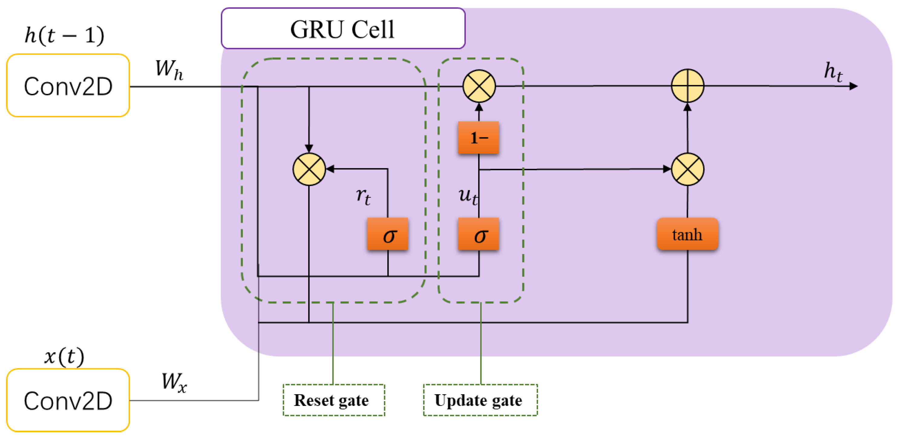
Similarly, in the ConvGRU diagram (Figure 6), the input is first processed through Conv2D, with convolutional layers that handle spatial information by applying filters to the input data. Within the GRU cell, there are two gates: the reset gate r t and the update gate u t . Both are responsible for determining how much of the past information needs to be passed along to the future. GRUs are similar to LSTMs in that they effectively capture temporal dependencies but with a simpler structure that combines the forget and input gates into a single update gate. This can make GRUs faster to train and can work better on less complex sequences.
In Figure 7, the initial stage is the CNN cell, which performs feature extraction for input X through a series of operations. It begins with convolutional layers that apply filters to the input to produce feature maps. This is followed by a ReLU (Rectified Linear Unit) activation function that introduces nonlinearity into the system, allowing the model to learn more complex patterns. Afterward, max pooling is applied to reduce the spatial dimensions of the feature maps, condensing the information and reducing the number of parameters. These processed features are then passed to the LSTM model. LSTM units are designed to remember long-term dependencies and can maintain information in memory for long periods.
Figure 8 follows the same initial steps in the CNN cell, with convolution, ReLU activation, and max pooling. Instead of passing the features to an LSTM, they are input into a GRU model.
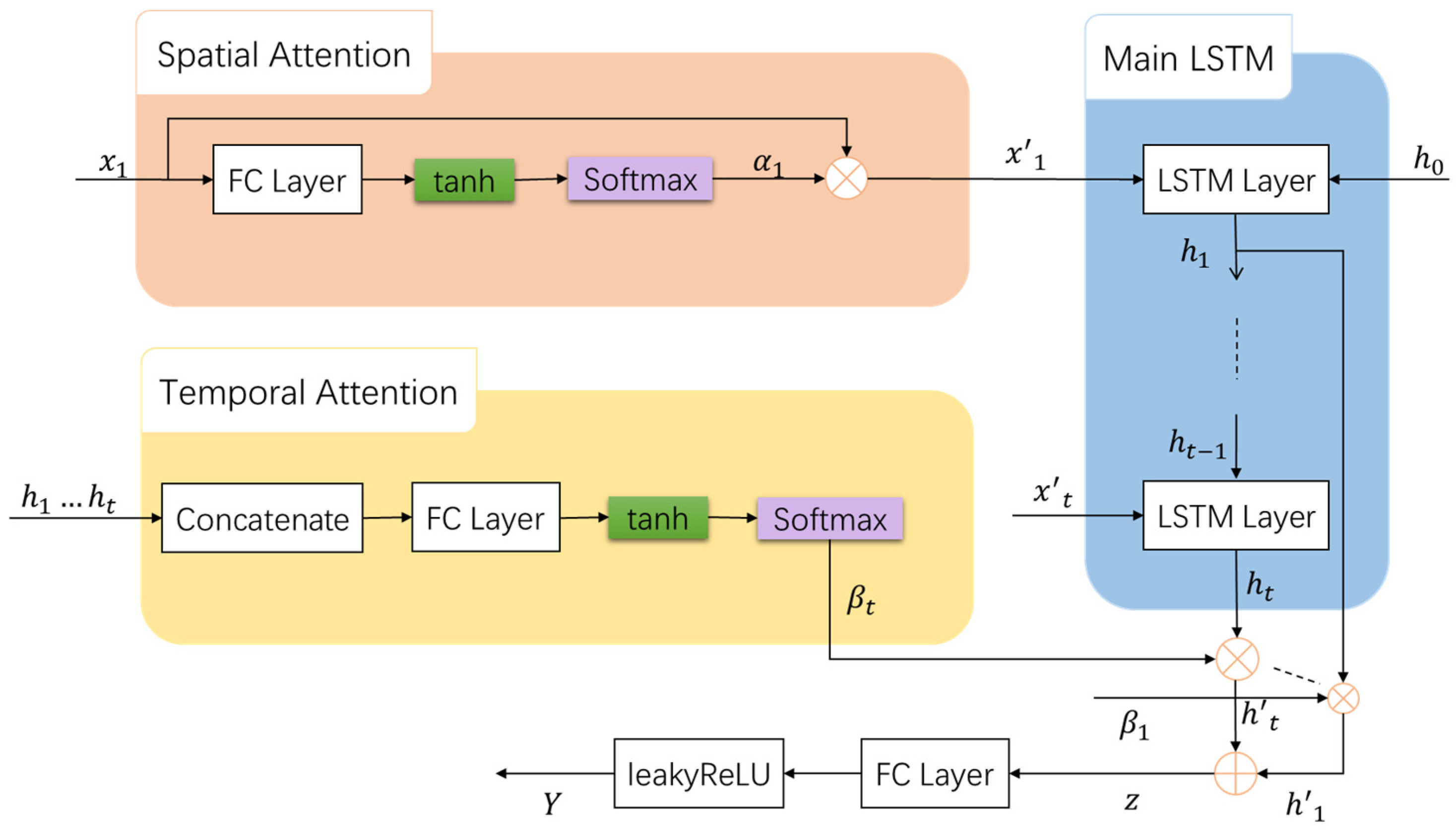
As shown in Figure 9, the STA-LSTM model’s architecture integrates spatial and temporal attention mechanisms with a traditional LSTM network to enhance predictive accuracy. The spatial attention mechanism, shown at the top, employs a Fully Connected (FC) layer followed by a tanh activation function and a softmax layer to compute the attention weights ( α 1 ), which prioritizes the input features spatially. The lower part of the diagram illustrates the temporal attention mechanism, which assigns importance weights ( β t ) to different time steps after concatenating the hidden states and processing them through an FC layer, a tanh activation function, and a softmax layer. These weights inform the main LSTM component of the model about the significance of each time step’s information. The output from both attention mechanisms is then integrated into the LSTM layers ( h 1 to h t ) to generate the final prediction.
To enhance the accuracy and computational efficiency of predictive models for streamflow prediction, our research proposes the integration of a GRU in place of LSTM units within the framework of an STA-LSTM model, thereby formulating an STA-GRU model. The rationale behind this substitution stems from the inherent advantages of GRUs over LSTMs, particularly in terms of computational simplicity and efficiency. GRUs simplify the recurrent unit architecture by merging the forget and input gates into a single update gate and eliminating the separate cell state, thereby reducing the model’s parameter count and, consequently, its computational overhead. This reduction in parameters not only accelerates the training process but also diminishes the computational resources required, making the model particularly advantageous for handling large datasets and facilitating rapid model iteration. Moreover, integrating spatial–temporal attention mechanisms within the GRU framework enables the STA-GRU model to more effectively identify and leverage critical temporal sequences and spatial locations that are pivotal for accurate streamflow forecasting.

2.2.1. STA-GRU Models

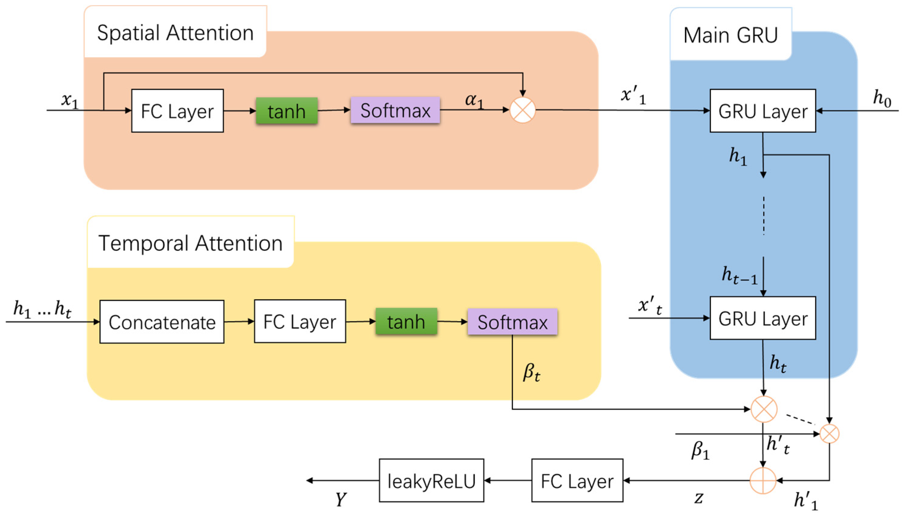
Figure 10 portrays a schematic representation of an advanced GRU network augmented with spatial and temporal attention mechanisms. This architecture is designed to enhance the model’s predictive capabilities by allowing it to focus on the most relevant features in the data.
Before feeding into the main GRU, the input x 1 (referring to the input at the first timestamp in a sequence being processed by the neural network) passes through a spatial attention mechanism, where it is first transformed by a Fully Connected (FC) layer. The output is then put through a tanh activation function, which normalizes the values between −1 and 1. The softmax function subsequently converts these values into a probability distribution α 1 , weighting the importance of each feature in the spatial domain. In the temporal attention part, it aims to assign different discharges of importance to different time steps of the GRU’s hidden states h 1 to h t . The hidden states are concatenated and processed through another FC layer, followed by a ReLU activation function. The softmax function then generates a set of weights β t , which are used to create a context vector that emphasizes the most informative time steps. The GRU layers are designed to remember long-term dependencies and mitigate the vanishing gradient problem that can occur with standard recurrent neural networks. The network processes the input sequence x t through time steps, updating its hidden state h t . The weighted hidden states from spatial and temporal attention mechanisms are combined to form a context vector z, which captures spatially and temporal relevant information. This vector is then passed through another FC layer and a Leaky ReLU activation function to predict the output Y.
This architecture is compelling for tasks that require understanding the importance of different input features at each time step (spatial attention) and the importance of different time steps in the input sequence (temporal attention). Combining these attention mechanisms with a GRU allows the network to make more informed predictions by effectively focusing on the most relevant information in both spatial and temporal dimensions. Replacing the LSTM layer with a GRU layer can enhance the overall computational efficiency of the model.

2.2.2. Evaluation Measures

In evaluating streamflow prediction models, accuracy and reliability are paramount metrics. To thoroughly assess model performance, researchers often employ various statistical measures [66]. The root mean square error (RMSE) and mean absolute error (MAE) are commonly used metrics that measure the mean of the squares and the absolute values of the deviations between predicted and actual values, respectively. The RMSE is more sensitive to larger errors, offering a more pronounced indication when model predictions are significantly off. In contrast, the MAE provides a linear error assessment, assigning equal weight to all deviations, which makes it more robust, particularly in the presence of outliers. R-square ( R 2 ) gives insight into the overall effectiveness of the model in explaining the variance observed in the actual data. Then, the mean absolute percentage error (MAPE) is a relative error metric that considers the magnitude of prediction errors about actual observations. These are particularly crucial in streamflow forecasting as they convey the percentage of prediction error relative to the actual measurements, providing decision makers with an intuitive understanding of the error magnitude [67].
  • The RMSE quantifies the average of the squares of the differences between predicted and actual observed values. It serves as a widely used metric for evaluating the accuracy of predictions.
    R M S E = 1 n i = 1 n ( O i P i ) 2
    where n is the number of observations, O i is the actual observed value, and P i is the predicted value.
  • The MAE represents the average absolute deviation between predicted values and actual observations, offering an intuitive gauge of predictive accuracy.
    M A E = i = 1 n O i P i n
  • The MAPE is a measure that expresses the accuracy of a predictive model as a percentage. It calculates the average absolute deviation between the observed values and the predictions relative to the actual values, thereby providing a clear and interpretable indication of the model’s prediction error in terms of proportionate accuracy.
    M A P E = ( 1 n i = 1 n O i P i O i ) × 100 %
  • R 2 is a measure that expresses the accuracy of a predictive model as a percentage. It calculates the average absolute deviation between the observed values and the predictions relative to the actual values, thereby providing a clear and interpretable indication of the model’s prediction error in terms of proportionate accuracy.
    R 2 = 1 i = 1 n ( O i P i ) 2 i = 1 n ( O i O ˜ i ) 2
Together, these statistical error metrics—RMSE, MAE, R-square, and MAPE—deliver a comprehensive analysis from diverse perspectives. The RMSE and MAE zero in on the magnitude of errors and mean accuracy, R-square sheds light on the model’s explanatory power, and MAPE assesses average absolute percentage errors. This integrated approach ensures a holistic evaluation, enhancing the ability to measure and optimize the efficacy of streamflow prediction models precisely.

3. Results and Discussion

Hyperparameter optimization plays a pivotal role in enhancing the performance of deep learning models. It involves the meticulous adjustment of parameters that dictate the training process of machine learning models. Such parameters include the learning rate, batch size, number of epochs, and the neural network’s architecture specifics, such as the number of layers and neurons per layer. Therefore, based on our dataset, the initial learning rate of the model is set at 0.0001, with a callback to adjust the learning rate during training. Given the complexity of our spatiotemporal forecasting model and the extensive number of features, we implemented regularization through the application of a dropout rate of 0.1 to mitigate the risk of overfitting. The models were trained with a batch size of 30 across 200 epochs to balance computational efficiency with the opportunity for adequate learning through iterative exposure to the training data.

3.1. Results and Analysis

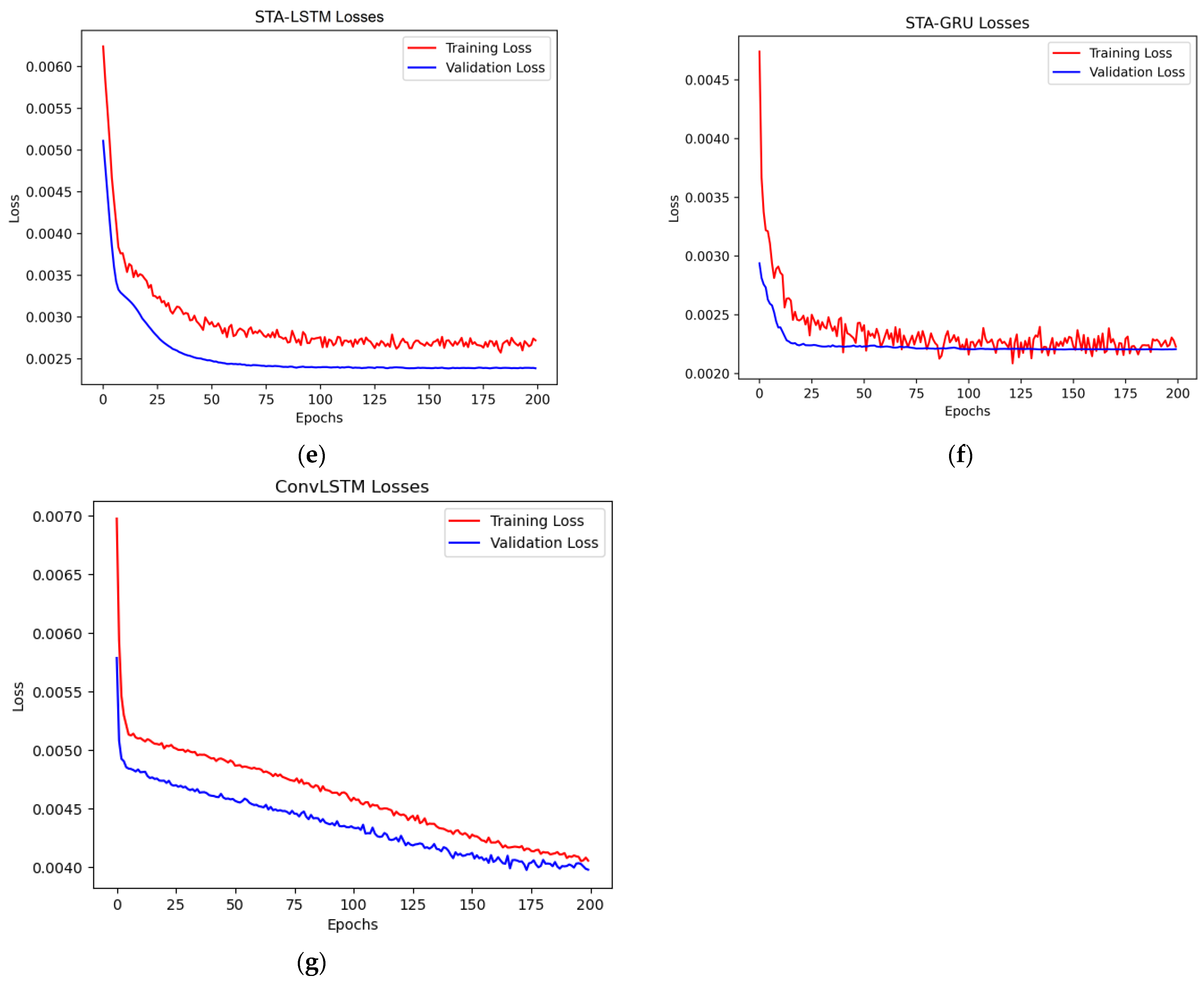
Figure 11 displays seven loss plots for different neural network models used in a machine learning context. These plots are a standard way to visualize the performance of a model during training and validation.
In Figure 11, the vertical axis represents the loss, which measures how well the model’s predictions match the actual data. The horizontal axis represents the training epochs, with full iterations over the entire dataset. An analysis of the loss plots for each model reveals a consistent pattern of rapid declines in training loss, indicative of practical learning phases, followed by stabilization, suggesting an adeptness at capturing data patterns without significant overfitting.
The LSTM model (a) demonstrates a swift decrease in training loss, with validation loss closely mirroring this trend, suggesting a robust pattern recognition capability. Similarly, the GRU model (b) exhibits a sharp reduction in training and validation loss, with the latter showing a smooth trend that signifies consistent validation performance. The CNNLSTM (c) and CNNGRU (d) models both show steep initial declines in training loss, with subsequent stabilization, albeit the CNNLSTM model presents more fluctuation in validation loss. This pattern suggests effective learning while maintaining an excellent fit to the data.
The STA-LSTM model depicted in the STA-LSTM Loss Plot (e) shows good learning behavior with a steady decrease in training and validation loss, suggesting that the model captures the underlying patterns without overfitting the training data. According to the STA-GRU loss plot (f), the STA-GRU model drastically reduces loss. The model performs well in both the convergence of training and validation loss, with no apparent signs of underfitting or overfitting, suggesting that the model effectively captures meaningful temporal relationships and has good generalization. The ConvLSTM loss plot (g) displays both the training and validation losses dropping sharply at the beginning, which is when the model learns from the data. As the epochs increase, both losses continue to decrease, but at a much slower rate, indicating that the model is gradually improving and learning from the training data. The overall loss plot trend shows a good fit.
All models seem to learn effectively, as indicated by the decrease in training loss. Most models also generalize well to the validation set, except for the ConvLSTM, which shows some instability in the validation loss. This could suggest that the ConvLSTM model might be overfitting to the training data or require further tuning or more data to achieve stable performance. Moreover, these models that manifest the lowest validation loss and demonstrate convergence with the training loss indicate superior generalization capabilities.

3.2. Discussions

In evaluating forecasting models over 1 and 7 day horizons, the performance metrics of the testing set and training set considered were the RMSE, MAE, MAPE, and R2, as shown in Table 3. A comparative analysis between the training and testing datasets reveals insights into model generalizability and the propensity for overfitting. The STA-GRU model consistently exhibited superior performance across all metrics and forecasting horizons, suggesting robustness and accuracy in its predictive capabilities. Notably, with a 7-day horizon, the STA-GRU model achieved the lowest RMSE (6.591 and 6.727), indicating minimal deviation from actual values, and a low MAE (3.450 and 3.653), reflecting the smallest average magnitude of error per prediction. Moreover, the model sustained the lowest MAPE (32.0% and 35.6%) and the highest R2 (37.7% and 31.2%), demonstrating the highest precision in terms of percentage error relative to the actual values. Then, the STA-GRU model shows consistent performance between training and testing with closely aligned RMSE and MAE values, suggesting reduced overfitting compared to other models that exhibit significant performance drops on the test set.
While the STA-LSTM model showed commendable performance, particularly with the lowest MAE (3.401 and 3.533) with a 7-day horizon, it did not consistently outperform across all metrics. This suggests that while STA-LSTM may be sensitive to certain error types, it may not capture the time-series dynamics as effectively as STA-GRU. Other models, including LSTM and the GRU, demonstrated competitive metrics in isolated instances but lacked consistent leadership. The convolutional models (CNNLSTM and CNNGRU) appeared to underperform in this task, especially in long-term forecasting.
The ConvLSTM model stands out for its average percentage error in short-term forecasting, but its long-term performance declines. Moreover, the STA-LSTM and STA-GRU models, which incorporate an attention mechanism, outperform the other hybrid LSTM and GRU models, suggesting that the attention mechanism may enhance forecasting performance.
Furthermore, when comparing our results presented in Table 3 with the results of other recent publications, presented in Table 1, the STA-GRU model manifests a notably enhanced predictive performance in a one-day-ahead temporal framework, as evidenced by its lower RMSE, MAE, and MAPE values, coupled with a superior R-square. This indicates that the STA-GRU model exhibits exceptional precision and reliability within the confines of a short-term forecasting horizon, outstripping the reference models listed in the table. Extending the prediction interval to 7 days ahead, the STA-GRU model consistently maintains commendable RMSE, MAE, MAPE, and R-square figures. This consistency in performance underscores the robustness of the STA-GRU model in both short-term and long-term hydrological predictions.
Figure 12 illustrates the model’s predictive proficiency for 1 day and 7 days ahead. It evidences the model’s commendable capacity to mirror the observed discharge trends closely, as indicated by the congruence between the observed data (blue line) and the predicted data (red line and black line), especially the low discharge. Notwithstanding, the model exhibits some discrepancies in capturing the extremities of the discharge spectrum, particularly the peak values. Despite these deviations, the model’s performance remains robust for short-term forecasting. For 7 days ahead, the model’s predictive trajectory, while still preserving the general discharge pattern, reveals a discernible divergence from the observed values, especially in peak flow periods. Nonetheless, this anticipated decrement in predictive accuracy over a longer forecasting horizon does not substantially diminish the model’s utility. The STA-GRU model maintains substantial reliability, capturing the overarching discharge trends despite the increased prediction uncertainty over an extended temporal scale.
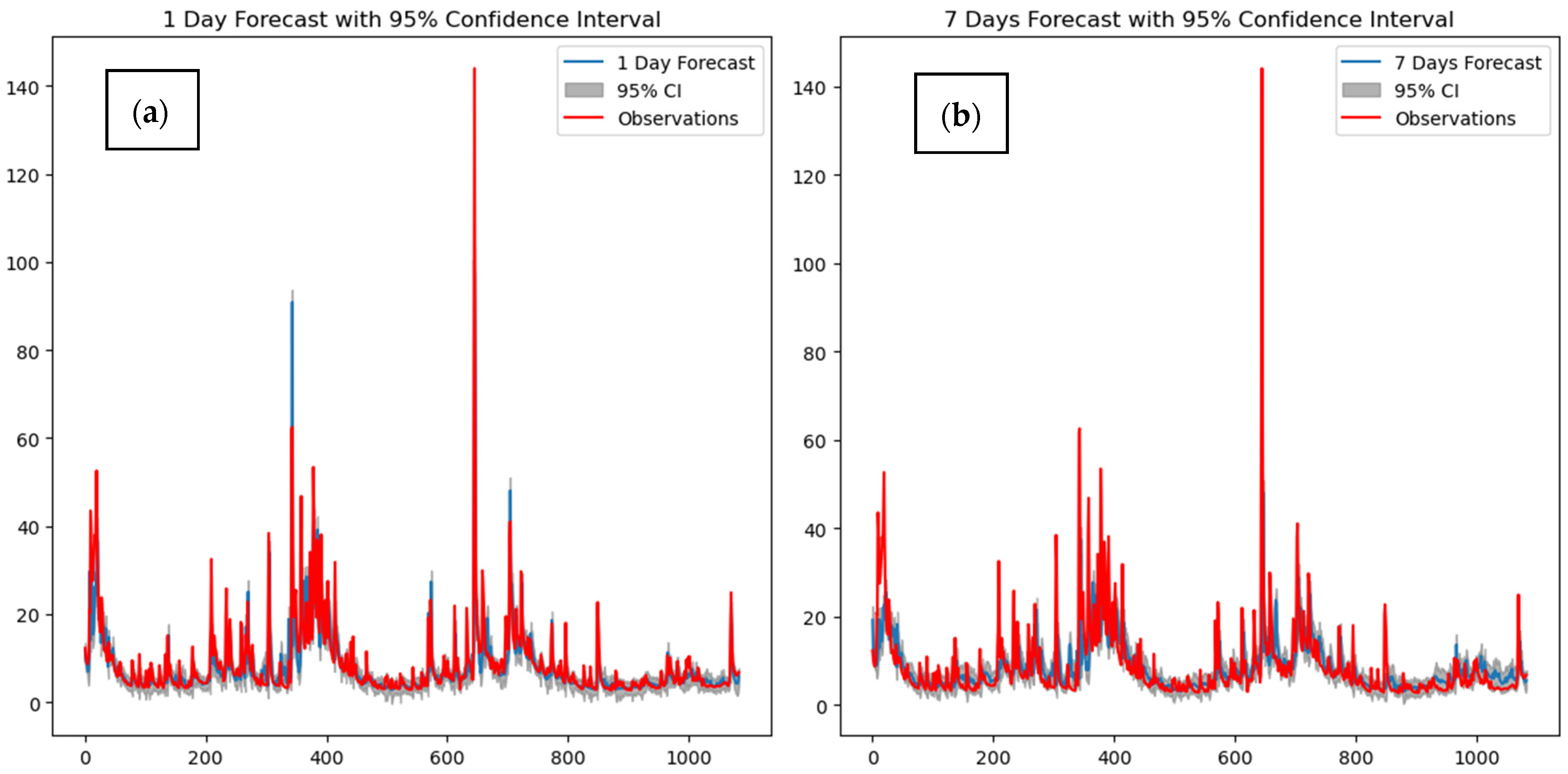
Figure 13 presents the uncertainty analysis of the Spatial–Temporal Attention-Gated Recurrent Unit (STA-GRU) model. Firstly, it is evident that as the forecast horizon extends from one to seven days, the uncertainty escalates, as indicated by the widening of the 95% confidence intervals. In other words, as the forecasting horizon lengthens, the uncertainty of the prediction model correspondingly increases.
Moreover, the presence of outliers appears to have a substantial impact on the model’s uncertainty. This is particularly noticeable where the confidence intervals significantly broaden at points where there is a considerable divergence between the predictions and the actual observations. Although the STA-GRU model is expected to capture most patterns accurately, its uncertainty increased when dealing with peak flows.
The STA-GRU model exhibited the lowest RMSE and MAE, a relatively low MAPE, and the highest R-square when predicting streamflow for the seventh day ahead. These indicators collectively point towards the superiority of the STA-GRU model in terms of predictive accuracy. Upon analyzing the Monte Carlo dropout uncertainty plots, the STA-GRU model sustains low predictive uncertainty across its outputs. Therefore, the STA-GRU model exhibits a promising predictive insight, with its efficacy being more pronounced in short-term predictions. Although slightly attenuated, the model’s performance in long-term forecasting retains its practical applicability, affirming its potential for integration into hydrological forecasting systems with acceptable margins of predictive uncertainty.

4. Conclusions

The advent of deep learning algorithms has substantially advanced the field of streamflow forecasting, particularly in enhancing the forecasting horizon. Our investigation delved into various deep learning architectures to refine streamflow forecasting techniques. This array included the foundational LSTM network and its spatially aware variants, such as CNNLSTM, ConvLSTM, and the STA-LSTM. Additionally, we explored the GRU and its cognate models, the CNNGRU and the innovative STA-GRU, to assess their efficacy in the complexities of hydrological datasets for streamflow prediction.
By capitalizing on spatial insights amalgamated with sequential data patterns, we aimed to construct a more integrative model for streamflow prediction. Our findings revealed that the spatial–temporal-attention-enabled models, such as STA-LSTM and STA-GRU, were proficient in handling the intricacies of long-term dependencies inherent in environmental data.
Moreover, we enhance the performance of deep learning methodologies by incorporating groundwater level station data alongside conventional precipitation and discharge station data. Integrating groundwater level data as a feature has notably improved the accuracy and consistency of our model’s predictions, particularly in predicting low flow conditions, thereby establishing a new standard for precision compared to related research in the field.
Notably, the STA-GRU model excelled in computational expediency while sustaining a predictive prowess comparable to that of STA-LSTM. This attribute of computational swiftness is pivotal in streamflow forecasting contexts, empowering the system to expeditiously analyze voluminous datasets, which is instrumental for prompt drought or flooding monitoring and response actions.
The capacity for rapid analysis not only aids in the timely dissemination of warnings but also supports the ongoing refinement of forecast models, thereby sharpening the precision of drought/flooding alerts. The STA-GRU and STA-LSTM models demonstrate an exceptional ability to prioritize crucial data points, yielding more precise streamflow predictions by capturing the nuanced spatio-temporal dynamics. These models stand at the vanguard of ongoing efforts to elevate the capabilities of streamflow forecasting for watershed management.
However, despite the advantages demonstrated by the STA-GRU model in both short-term and long-term forecasting scenarios, it also exhibited certain limitations. Firstly, the model’s generalization and applicability are the primary limitations. In short-term (1 day) forecasts, the performance gains of STA-GRU were relatively moderate compared to those of ConvLSTM and STA-LSTM, suggesting that the benefits of the attention mechanism might be limited when dealing with specific datasets. Then, in the context of long-term (7 day) forecasts, although STA-GRU outperformed other models, it did not exhibit a significantly superior lead similar to its short-term predictions, which may reflect the model’s challenges in managing dependencies over longer time sequences. Perhaps the inclusion of additional features could bolster the model’s capacity to elucidate the complex underpinnings of hydrological processes. This is because the opacity inherent in the black-box nature of machine learning models curtails the depth of interpretability.
In conclusion, our research highlights the potential of deep learning algorithms to enhance the accuracy and scope of streamflow forecasting, particularly by adopting spatial–temporal attention mechanisms and integrating diverse data sources. Moreover, the profound practical implications of enhancing streamflow forecasting accuracy through the integration of groundwater level data and the application of advanced spatial–temporal attention models, particularly the STA-GRU model. The findings bear significant relevance to drought management, enabling more accurate predictions that can inform effective water allocation strategies, irrigation planning, and conservation efforts. Such advancements are crucial for mitigating the adverse effects of drought on agriculture, ecosystems, and water security. Furthermore, the application of these methodologies extends to improved flood risk management, offering the potential for more accurate high-flow predictions that are essential for emergency planning and mitigation strategies. Despite some limitations, STA-GRU and other advanced models continue to offer significant directions for progress in hydrological forecasting and management.

Author Contributions

Conceptualization: Y.Z. and B.G.; methodology: Y.Z., B.G., Z.Z. and Y.D.; software: J.V.G.T., Y.Z. and D.P.; validation: Y.Z.; formal analysis: Y.Z.; investigation: Y.Z.; resources: Y.Z. and B.G.; data curation: Y.Z.; writing—original draft preparation: Y.Z., B.G., J.V.G.T. and S.X.Y.; writing—review and editing: B.G., J.V.G.T. and S.X.Y.; supervision: B.G. and S.X.Y.; project administration: B.G., S.X.Y. and J.V.G.T.; funding acquisition: B.G. and J.V.G.T. All authors have read and agreed to the published version of the manuscript.

Funding

This research was funded by the Natural Sciences and Engineering Research Council of Canada (NSERC) with Alliance Grant #401643, with support from Lakes Environmental Software Inc.

Data Availability Statement

The datasets used in this study are in the public domain and are available for download from the Water Survey of Canada (for the Discharge), the Ontario Ministry of the Environment Provincial Groundwater Monitoring Program (for the Groundwater Level Data) and Environment Canada (for the Precipitation data).

Conflicts of Interest

Author Jesse Van Griensven is employed by the company Lakes Software. The remaining authors declare that the research was conducted in the absence of any commercial or financial relationships that could be construed as a potential conflict of interest.

References

  1. Bhasme, P.; Bhatia, U. Improving the interpretability and predictive power of hydrological models: Applications for daily streamflow in managed and unmanaged catchments. J. Hydrol. 2024, 628, 130421. [Google Scholar] [CrossRef]
  2. Drisya, J.; Kumar, D.S.; Roshni, T. Hydrological drought assessment through streamflow forecasting using wavelet enable artificial neural networks. Environ. Dev. Sustain. 2021, 23, 3653–3672. [Google Scholar] [CrossRef]
  3. Tan, M.L.; Gassman, P.W.; Yang, X.; Haywood, J. A review of SWAT applications, performance and future needs for simulation of hydro-climatic extremes. Adv. Water Resour. 2020, 143, 103662. [Google Scholar] [CrossRef]
  4. Jahangir, M.S.; Quilty, J. Generative deep learning for probabilistic streamflow forecasting: Conditional variational auto-encoder. J. Hydrol. 2024, 629, 130498. [Google Scholar] [CrossRef]
  5. Kumar, V.; Kedam, N.; Sharma, K.V.; Mehta, D.J.; Caloiero, T. Advanced machine learning techniques to improve hydrological prediction: A comparative analysis of streamflow prediction models. Water 2023, 15, 2572. [Google Scholar] [CrossRef]
  6. Sabale, R.; Venkatesh, B.; Jose, M. Sustainable water resource management through conjunctive use of groundwater and surface water: A review. Innov. Infrastruct. Solut. 2023, 8, 17. [Google Scholar] [CrossRef]
  7. Tripathy, K.P.; Mishra, A.K. Deep Learning in Hydrology and Water Resources Disciplines: Concepts, Methods, Applications, and Research Directions. J. Hydrol. 2023, 628, 130458. [Google Scholar] [CrossRef]
  8. Yildirim, I.; Aksoy, H. Intermittency as an indicator of drought in streamflow and groundwater. Hydrol. Process. 2022, 36, e14615. [Google Scholar] [CrossRef]
  9. Wang, T.; Wu, Z.; Wang, P.; Wu, T.; Zhang, Y.; Yin, J.; Yu, J.; Wang, H.; Guan, X.; Xu, H.; et al. Plant-groundwater interactions in drylands: A review of current research and future perspectives. Agric. For. Meteorol. 2023, 341, 109636. [Google Scholar] [CrossRef]
  10. Meng, F.; Luo, M.; Sa, C.; Wang, M.; Bao, Y. Quantitative assessment of the effects of climate, vegetation, soil and groundwater on soil moisture spatiotemporal variability in the Mongolian Plateau. Sci. Total Environ. 2022, 809, 152198. [Google Scholar] [CrossRef] [PubMed]
  11. Han, Z.; Huang, S.; Huang, Q.; Bai, Q.; Leng, G.; Wang, H.; Zhao, J.; Wei, X.; Zheng, X. Effects of vegetation restoration on groundwater drought in the Loess Plateau, China. J. Hydrol. 2020, 591, 125566. [Google Scholar] [CrossRef]
  12. Marchionni, V.; Daly, E.; Manoli, G.; Tapper, N.; Walker, J.; Fatichi, S. Groundwater buffers drought effects and climate variability in urban reserves. Water Resour. Res. 2020, 56, e2019WR026192. [Google Scholar] [CrossRef]
  13. Gavrilescu, M. Water, soil, and plants interactions in a threatened environment. Water 2021, 13, 2746. [Google Scholar] [CrossRef]
  14. Ondrasek, G.; Rengel, Z. Environmental salinization processes: Detection, implications & solutions. Sci. Total Environ. 2021, 754, 142432. [Google Scholar] [PubMed]
  15. Mukhopadhyay, R.; Sarkar, B.; Jat, H.S.; Sharma, P.C.; Bolan, N.S. Soil salinity under climate change: Challenges for sustainable agriculture and food security. J. Environ. Manag. 2021, 280, 111736. [Google Scholar] [CrossRef]
  16. Stavi, I.; Thevs, N.; Priori, S. Soil salinity and sodicity in drylands: A review of causes, effects, monitoring, and restoration measures. Front. Environ. Sci. 2021, 9, 712831. [Google Scholar] [CrossRef]
  17. Lee, S.; Hyun, Y.; Lee, S.; Lee, M.J. Groundwater potential mapping using remote sensing and GIS-based machine learning techniques. Remote Sens. 2020, 12, 1200. [Google Scholar] [CrossRef]
  18. Abdelkareem, M.; Al-Arifi, N. The use of remotely sensed data to reveal geologic, structural, and hydrologic features and predict potential areas of water resources in arid regions. Arab. J. Geosci. 2021, 14, 1–15. [Google Scholar] [CrossRef]
  19. Gholami, V.; Booij, M. Use of machine learning and geographical information system to predict nitrate concentration in an unconfined aquifer in Iran. J. Clean. Prod. 2022, 360, 131847. [Google Scholar] [CrossRef]
  20. Drogkoula, M.; Kokkinos, K.; Samaras, N. A Comprehensive Survey of Machine Learning Methodologies with Emphasis in Water Resources Management. Appl. Sci. 2023, 13, 12147. [Google Scholar] [CrossRef]
  21. Ntona, M.M.; Busico, G.; Mastrocicco, M.; Kazakis, N. Modeling groundwater and surface water interaction: An overview of current status and future challenges. Sci. Total Environ. 2022, 846, 157355. [Google Scholar] [CrossRef] [PubMed]
  22. Haque, A.; Salama, A.; Lo, K.; Wu, P. Surface and groundwater interactions: A review of coupling strategies in detailed domain models. Hydrology 2021, 8, 35. [Google Scholar] [CrossRef]
  23. Condon, L.E.; Kollet, S.; Bierkens, M.F.; Fogg, G.E.; Maxwell, R.M.; Hill, M.C.; Fransen, H.J.H.; Verhoef, A.; Van Loon, A.F.; Sulis, M.; et al. Global groundwater modeling and monitoring: Opportunities and challenges. Water Resour. Res. 2021, 57, e2020WR029500. [Google Scholar] [CrossRef]
  24. Wang, W.; Van Gelder, P.H.; Vrijling, J.; Ma, J. Forecasting daily streamflow using hybrid ANN models. J. Hydrol. 2006, 324, 383–399. [Google Scholar] [CrossRef]
  25. Rasouli, K.; Hsieh, W.W.; Cannon, A.J. Daily streamflow forecasting by machine learning methods with weather and climate inputs. J. Hydrol. 2012, 414, 284–293. [Google Scholar] [CrossRef]
  26. Cheng, M.; Fang, F.; Kinouchi, T.; Navon, I.; Pain, C. Long lead-time daily and monthly streamflow forecasting using machine learning methods. J. Hydrol. 2020, 590, 125376. [Google Scholar] [CrossRef]
  27. Chu, H.; Wei, J.; Wu, W.; Jiang, Y.; Chu, Q.; Meng, X. A classification-based deep belief networks model framework for daily streamflow forecasting. J. Hydrol. 2021, 595, 125967. [Google Scholar] [CrossRef]
  28. Essam, Y.; Huang, Y.F.; Ng, J.L.; Birima, A.H.; Ahmed, A.N.; El-Shafie, A. Predicting streamflow in Peninsular Malaysia using support vector machine and deep learning algorithms. Sci. Rep. 2022, 12, 3883. [Google Scholar] [CrossRef] [PubMed]
  29. Ibrahim, K.S.M.H.; Huang, Y.F.; Ahmed, A.N.; Koo, C.H.; El-Shafie, A. A review of the hybrid artificial intelligence and optimization modelling of hydrological streamflow forecasting. Alex. Eng. J. 2022, 61, 279–303. [Google Scholar] [CrossRef]
  30. Riahi-Madvar, H.; Dehghani, M.; Memarzadeh, R.; Gharabaghi, B. Short to long-term forecasting of river flows by heuristic optimization algorithms hybridized with ANFIS. Water Resour. Manag. 2021, 35, 1149–1166. [Google Scholar] [CrossRef]
  31. Sit, M.; Demiray, B.Z.; Xiang, Z.; Ewing, G.J.; Sermet, Y.; Demir, I. A comprehensive review of deep learning applications in hydrology and water resources. Water Sci. Technol. 2020, 82, 2635–2670. [Google Scholar] [CrossRef] [PubMed]
  32. Ardabili, S.; Mosavi, A.; Dehghani, M.; Várkonyi-Kóczy, A.R. Deep learning and machine learning in hydrological processes climate change and earth systems a systematic review. In Proceedings of the Engineering for Sustainable Future: Selected Papers of the 18th International Conference on Global Research and Education Inter-Academia–2019 18, Budapest and Balatonfüred, Hungary, 4–7 September 2019; Springer: Berlin/Heidelberg, Germany, 2020; pp. 52–62. [Google Scholar]
  33. Ruma, J.F.; Adnan, M.S.G.; Dewan, A.; Rahman, R.M. Particle swarm optimization based LSTM networks for water level forecasting: A case study on Bangladesh river network. Results Eng. 2023, 17, 100951. [Google Scholar] [CrossRef]
  34. Xiang, Z.; Yan, J.; Demir, I. A rainfall-runoff model with LSTM-based sequence-to-sequence learning. Water Resour. Res. 2020, 56, e2019WR025326. [Google Scholar] [CrossRef]
  35. Song, X.; Liu, Y.; Xue, L.; Wang, J.; Zhang, J.; Wang, J.; Jiang, L.; Cheng, Z. Time-series well performance prediction based on Long Short-Term Memory (LSTM) neural network model. J. Pet. Sci. Eng. 2020, 186, 106682. [Google Scholar] [CrossRef]
  36. Duan, J.; Zhang, P.F.; Qiu, R.; Huang, Z. Long short-term enhanced memory for sequential recommendation. World Wide Web 2023, 26, 561–583. [Google Scholar] [CrossRef]
  37. Sagheer, A.; Hamdoun, H.; Youness, H. Deep LSTM-based transfer learning approach for coherent forecasts in hierarchical time series. Sensors 2021, 21, 4379. [Google Scholar] [CrossRef] [PubMed]
  38. Feng, D.; Fang, K.; Shen, C. Enhancing streamflow forecast and extracting insights using long-short term memory networks with data integration at continental scales. Water Resour. Res. 2020, 56, e2019WR026793. [Google Scholar] [CrossRef]
  39. Fu, M.; Fan, T.; Ding, Z.; Salih, S.Q.; Al-Ansari, N.; Yaseen, Z.M. Deep learning data-intelligence model based on adjusted forecasting window scale: Application in daily streamflow simulation. IEEE Access 2020, 8, 32632–32651. [Google Scholar] [CrossRef]
  40. Li, G.; Zhu, H.; Jian, H.; Zha, W.; Wang, J.; Shu, Z.; Yao, S.; Han, H. A combined hydrodynamic model and deep learning method to predict water level in ungauged rivers. J. Hydrol. 2023, 625, 130025. [Google Scholar] [CrossRef]
  41. Ghimire, S.; Yaseen, Z.M.; Farooque, A.A.; Deo, R.C.; Zhang, J.; Tao, X. Streamflow prediction using an integrated methodology based on convolutional neural network and long short-term memory networks. Sci. Rep. 2021, 11, 17497. [Google Scholar] [CrossRef] [PubMed]
  42. Vatanchi, S.M.; Etemadfard, H.; Maghrebi, M.F.; Shad, R. A comparative study on forecasting of long-term daily streamflow using ANN, ANFIS, BiLSTM and CNN-GRU-LSTM. Water Resour. Manag. 2023, 37, 4769–4785. [Google Scholar] [CrossRef]
  43. Soltani, K.; Ebtehaj, I.; Amiri, A.; Azari, A.; Gharabaghi, B.; Bonakdari, H. Mapping the spatial and temporal variability of flood susceptibility using remotely sensed normalized difference vegetation index and the forecasted changes in the future. Sci. Total Environ. 2021, 770, 145288. [Google Scholar] [CrossRef]
  44. Mohammed, A.; Corzo, G. Spatiotemporal convolutional long short-term memory for regional streamflow predictions. J. Environ. Manag. 2024, 350, 119585. [Google Scholar] [CrossRef] [PubMed]
  45. Baek, S.S.; Pyo, J.; Chun, J.A. Prediction of water level and water quality using a CNN-LSTM combined deep learning approach. Water 2020, 12, 3399. [Google Scholar] [CrossRef]
  46. Verma, S.; Srivastava, K.; Tiwari, A.; Verma, S. Deep learning techniques in extreme weather events: A review. arXiv 2023, arXiv:2308.10995. [Google Scholar]
  47. Dehghani, A.; Moazam, H.M.Z.H.; Mortazavizadeh, F.; Ranjbar, V.; Mirzaei, M.; Mortezavi, S.; Ng, J.L.; Dehghani, A. Comparative evaluation of LSTM, CNN, and ConvLSTM for hourly short-term streamflow forecasting using deep learning approaches. Ecol. Inform. 2023, 75, 102119. [Google Scholar] [CrossRef]
  48. Ding, Y.; Zhu, Y.; Feng, J.; Zhang, P.; Cheng, Z. Interpretable spatio-temporal attention LSTM model for flood forecasting. Neurocomputing 2020, 403, 348–359. [Google Scholar] [CrossRef]
  49. Cho, M.; Kim, C.; Jung, K.; Jung, H. Water level prediction model applying a long short-term memory (lstm)–gated recurrent unit (gru) method for flood prediction. Water 2022, 14, 2221. [Google Scholar] [CrossRef]
  50. Xu, W.; Chen, J.; Zhang, X.J. Scale effects of the monthly streamflow prediction using a state-of-the-art deep learning model. Water Resour. Manag. 2022, 36, 3609–3625. [Google Scholar] [CrossRef]
  51. Alizadeh, B.; Bafti, A.G.; Kamangir, H.; Zhang, Y.; Wright, D.B.; Franz, K.J. A novel attention-based LSTM cell post-processor coupled with bayesian optimization for streamflow prediction. J. Hydrol. 2021, 601, 126526. [Google Scholar] [CrossRef]
  52. Zhao, X.; Lv, H.; Wei, Y.; Lv, S.; Zhu, X. Streamflow forecasting via two types of predictive structure-based gated recurrent unit models. Water 2021, 13, 91. [Google Scholar] [CrossRef]
  53. Wegayehu, E.B.; Muluneh, F.B. Multivariate streamflow simulation using hybrid deep learning models. Comput. Intell. Neurosci. 2021, 2021, 5172658. [Google Scholar] [CrossRef] [PubMed]
  54. Jamei, M.; Jamei, M.; Ali, M.; Karbasi, M.; Farooque, A.A.; Malik, A.; Cheema, S.J.; Esau, T.J.; Yaseen, Z.M. Quantitative improvement of streamflow forecasting accuracy in the Atlantic zones of Canada based on hydro-meteorological signals: A multi-level advanced intelligent expert framework. Ecol. Inform. 2024, 80, 102455. [Google Scholar] [CrossRef]
  55. Zhang, Y.; Zhou, Z.; Van Griensven Thé, J.; Yang, S.X.; Gharabaghi, B. Flood Forecasting Using Hybrid LSTM and GRU Models with Lag Time Preprocessing. Water 2023, 15, 3982. [Google Scholar] [CrossRef]
  56. Tarekegn, A.N.; Ullah, M.; Cheikh, F.A. Deep Learning for Multi-Label Learning: A Comprehensive Survey. arXiv 2024, arXiv:2401.16549. [Google Scholar]
  57. Mhedhbi, R. Integrating Precipitation Nowcasting in a Deep Learning-Based Flash Flood Prediction Framework and Assessing the Impact of Rainfall Forecasts Uncertainties. Master’s Thesis, York University, Toronto, ON, Canada, 2022. [Google Scholar]
  58. Suthar, T.; Shah, T.; Raja, M.K.; Raha, S.; Kumar, A.; Ponnusamy, M. Predicting Weather Forecast Uncertainty based on Large Ensemble of Deep Learning Approach. In Proceedings of the 2023 International Conference on Self Sustainable Artificial Intelligence Systems (ICSSAS), Erode, India, 18–20 October 2023; pp. 1–6. [Google Scholar]
  59. Landi, F.; Baraldi, L.; Cornia, M.; Cucchiara, R. Working memory connections for LSTM. Neural Netw. 2021, 144, 334–341. [Google Scholar] [CrossRef] [PubMed]
  60. Zhang, Y.; Gu, Z.; Thé, J.V.G.; Yang, S.X.; Gharabaghi, B. The discharge forecasting of multiple monitoring station for humber river by hybrid LSTM models. Water 2022, 14, 1794. [Google Scholar] [CrossRef]
  61. Niu, Z.; Zhong, G.; Yu, H. A review on the attention mechanism of deep learning. Neurocomputing 2021, 452, 48–62. [Google Scholar] [CrossRef]
  62. Li, X.; Zhang, W.; Ding, Q. Understanding and improving deep learning-based rolling bearing fault diagnosis with attention mechanism. Signal Process. 2019, 161, 136–154. [Google Scholar] [CrossRef]
  63. Ficklin, D.L.; Abatzoglou, J.T.; Robeson, S.M.; Null, S.E.; Knouft, J.H. Natural and managed watersheds show similar responses to recent climate change. Proc. Natl. Acad. Sci. USA 2018, 115, 8553–8557. [Google Scholar] [CrossRef] [PubMed]
  64. Ficklin, D.L.; Luo, Y.; Luedeling, E.; Zhang, M. Climate change sensitivity assessment of a highly agricultural watershed using SWAT. J. Hydrol. 2009, 374, 16–29. [Google Scholar] [CrossRef]
  65. Heerspink, B.P.; Kendall, A.D.; Coe, M.T.; Hyndman, D.W. Trends in streamflow, evapotranspiration, and groundwater storage across the Amazon Basin linked to changing precipitation and land cover. J. Hydrol. Reg. Stud. 2020, 32, 100755. [Google Scholar] [CrossRef]
  66. Kumar, S.; Kolekar, T.; Kotecha, K.; Patil, S.; Bongale, A. Performance evaluation for tool wear prediction based on Bi-directional, Encoder–Decoder and Hybrid Long Short-Term Memory models. Int. J. Qual. Reliab. Manag. 2022, 39, 1551–1576. [Google Scholar] [CrossRef]
  67. Zhang, Y.; Pan, D.; Van Griensven, J.; Yang, S.X.; Gharabaghi, B. Intelligent flood forecasting and warning: A survey. Intell. Robot 2023, 3, 190–212. [Google Scholar] [CrossRef]
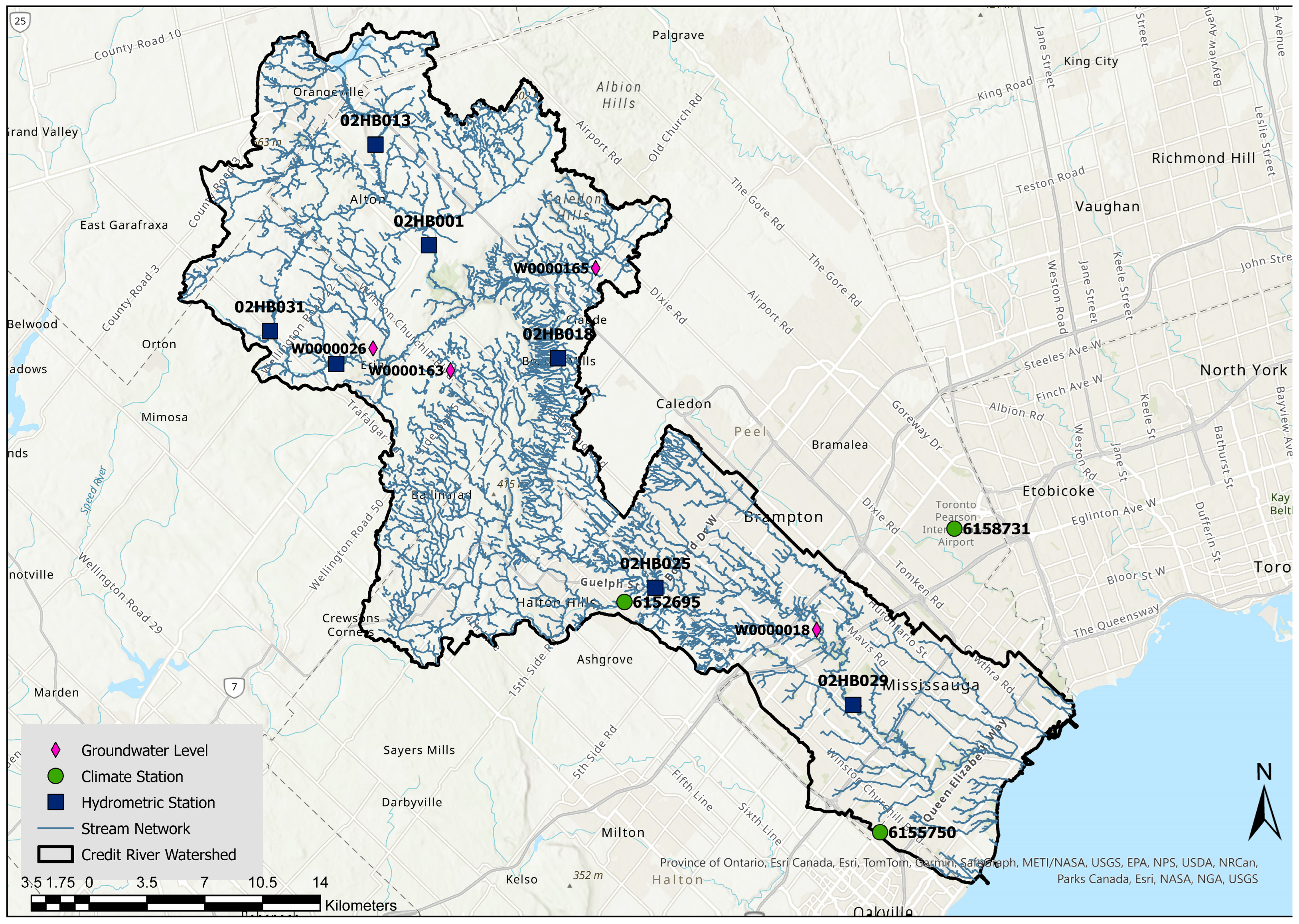
Figure 1. The real-time monitoring stations in the Credit River Watershed.
Water 16 01284 g001
Figure 2. Peak values for discharge stations and groundwater level stations.
Water 16 01284 g002
Figure 3. Matrix plot of Pearson correlations between the precipitation, discharge, and groundwater level.
Water 16 01284 g003
Figure 4. SHAP summary plot among the precipitation, discharge, and groundwater level stations.
Water 16 01284 g004
Figure 5. ConvLSTM model’s structure.
Water 16 01284 g005
Figure 6. ConvGRU model’s structure.
Water 16 01284 g006
Figure 7. CNNLSTM model’s structure.
Water 16 01284 g007
Figure 8. CNNGRU model’s structure.
Water 16 01284 g008
Figure 9. STA-LSTM model’s structure.
Water 16 01284 g009
Figure 10. STA-GRU model’s structure.
Water 16 01284 g010
Figure 11. The models’ training and validation error.
Water 16 01284 g011aWater 16 01284 g011b
Figure 12. Evaluation measures for the seven prediction models.
Water 16 01284 g012
Figure 13. MC dropout uncertainty for (a) one-day-ahead forecasting and (b) seven-day-ahead forecasting.
Water 16 01284 g013
Table 1. The performance of streamflow prediction models.
ReferenceModel RMSEMAE R 2
Chu, Haibo et al. (2021) [27]DBN43.0412.420.82
FCN-PMI-DBN26.518.080.95
Wegayehu et al. (2021) [53]GRU46.6320.890.55
CNNGRU45.6121.790.57
LSTM48.6422.790.51
CNNLSTM45.3821.850.57
Vatanchi et al. (2023) [42]ANFISN/A26.170.93
BiLSTMN/A32.150.92
Table 2. The statistics for the hydrometric, groundwater, and precipitation station dataset.
StationsMaxMinMeanStdStd/Mean
DC29144.002.009.068.680.958
DC25101.001.927.476.690.896
DC1860.801.704.943.740.757
DC206.320.210.510.310.608
DC311.480.110.170.050.294
DC0127.100.662.101.570.748
DC139.330.200.690.540.783
GW163426.13422.27424.440.790.002
GW018449.77447.67448.840.310.001
GW026390.20386.37387.330.640.002
GW165281.53279.92280.770.300.001
P615269573.600.001.324.273.235
P6158731126.000.002.215.612.538
P615575062.800.002.225.672.554
Table 3. The evaluation measures for the seven prediction models.
Forecast AlgorithmRMSE (Train)RMSE (Test)MAE (Train)MAE (Test)MAPE (Train)MAPE (Test) R 2
(Train)
R 2
(Test)
1LSTM7.2257.4483.5023.81746.7%47.5%30.1%21.2%
1GRU7.1017.1983.4733.77543.6%46.7%32.9%22.8%
1CNNLSTM6.7967.7423.2113.87937.4%48.0%40.6%14.9%
1CNNGRU6.6786.8962.2842.49037.0%47.5%39.8%22.6%
1ConvLSTM4.0264.5751.9651.99319.6%23.0%74.3%68.5%
1STA-LSTM4.2634.9392.1962.43923.1%25.1%78.6%71.6%
1STA-GRU3.7314.2142.0162.36219.2%21.5%80.2%74.4%
7LSTM7.5787.7553.7893.90549.1%52.8%20.2%14.5%
7GRU7.5317.7033.6993.87147.3%51.3%24.2%17.8%
7CNNLSTM7.7967.9353.4814.11740.9%53.1%28.9%10.1%
7CNNGRU7.3517.6363.4593.67939.6%41.9%29.1%16.7%
7ConvLSTM7.0817.4533.4373.74441.5%46.9%32.9%20.9%
7STA-LSTM6.7496.8993.4013.53338.6%40.6%36.0%28.3%
7STA-GRU6.5916.7273.4503.65332.0%35.6%37.7%31.2%
Disclaimer/Publisher’s Note: The statements, opinions and data contained in all publications are solely those of the individual author(s) and contributor(s) and not of MDPI and/or the editor(s). MDPI and/or the editor(s) disclaim responsibility for any injury to people or property resulting from any ideas, methods, instructions or products referred to in the content.