1. Introduction and Background
Dams, like any other infrastructure, respond to external and internal loads. The anisotropy and evolution of the mechanical properties of the materials they are composed of and their foundations make the whole system complex and evolutionary.
The mechanical response of the dam to variations in external variables exhibits reversible behaviour as long as the materials remain in the elastic zone. However, plasticization of materials, rheological changes, expansive chemical reactions, or degradation due to external factors impose irreversible deformations. Identification and definition of these trends are key to dam safety.
Traditional tools for trend detection in time series, such as dam monitoring data, are based on univariate analysis. A large number of scientific references on this topic can be found applied to various fields [
1,
2,
3].
These methods, as univariate, do not consider possible trends in loads as the temperature increases or the water levels decrease due to global climate change. Therefore, the trends of the behavioural variables of a dam defined by such univariate models may be influenced by the trends that the causal variables may exhibit and, consequently, may not adequately reflect the irreversible variations in its structural response mode, leading to a misinterpretation of the structural health of the dam.
Therefore, it is necessary to identify irreversible variations in the dam response (trends) using models that consider both behavioural variables and loads.
The most common models that relate causal and behavioural variables in current practice for dam safety monitoring are statistical models such as HST, HTT, variants thereof, or other types of multiple linear regression [
4,
5].
Numerical models, because of the significant heterogeneity of materials and complexity of the physical processes governing the dam’s response to external solicitations, as well as their high computational cost, are less widely used in monitoring instrumentation data.
The use of artificial intelligence (AI) models applied to dam safety has proliferated in recent times. Numerous scientific references related to the use of ML, DL, or hybrid models with other types of models such as statistical, time series, or physics-based numerical models can be found [
6,
7,
8,
9,
10,
11,
12]. Machine Learning models have shown good performance in monitoring data prediction and are more accessible to interpretation than DL models. However, despite the fact that these types of models generally provide better accuracy in predictions than any of the former, the practical application of such models is currently far from commonplace. This may be due to their label as black-box models.
For the consideration of irreversible effects attributable solely to the time variable, statistical models incorporate a series of terms that depend exclusively on this variable. The response part corresponding to these terms is then interpreted as the trend in the behaviour of the target variable. If the actual trend does not correspond to the shape of the function incorporated in the regression through the terms dependent on the time variable, the irreversible behaviour obtained with the model will lead to a misinterpretation of the structural response, not only because it cannot adjust to the actual trend, but also because it affects the coefficients of the other terms during least squares fitting.
Behaviour models based on Machine Learning do not impose any predetermined form of relationship between variables on the model and can incorporate time as just another feature among the dataset with which they are trained. In this way, data-driven models based on Machine Learning can learn, during their training stage and from monitoring data, how the dam’s response changes over time while considering the rest of the causal variables at the same time.
In these black-box models, the interpretation of the relationships between different variables and the target variable is not direct, as it is in statistical models, and requires specific methods. In the literature, multiple references can be found on the interpretation or explanation of these types of complex models.
Cortez et al. [
13], proposed different Sensitivity Analysis (SA) methods mainly focused on determining the importance of the inputs. He suggested the use of a Variable Effect Characteristic (VEC) curve to visualise the average impact of a given input in the model response based on the mean or median values of the rest of the inputs.
Based on this work, Lin et al. [
14] proposed a method for explanation of an Optimized Sparse Bayesian Learning. The explanation was focused on the relative importance of the input variables.
Lundberg et al. [
15] presented the Shapley Additive Explanations (SHAP) method to interpret predictions in complex models. Based on additive feature attribution methods and game theory, SHAP values provide the expected change in model prediction when a particular feature is conditioned.
Shao et al. [
16] used SHAP methods to evaluate the importance of factors involved in a multiple monitoring point (MMP) model orientated to predict settlements in a CFRD dam and to gain control of the settlement trends in this type of dam.
Tursunalieva et al. (2024) [
17] conducted a review of techniques for interpreting ML models, fundamentally classifying them into different categories: model-based, representation-based, and post hoc models. Within this latter group, they include methods such as the aforementioned SHAP, the Local Interpretable Model-Agnostic Explanations (LIME) introduced by Ribeiro et al. (2016) [
18], or the GradCAM focused on Deep Learning models proposed by Selvaraju et al. (2019) [
19], as model explanation techniques that allow understanding the logic behind complex ML models.
Individual Conditional Expectation curves (ICE), introduced by Goldstein (2015) [
20], are a visual tool used in the analysis of regression models to understand the relationship between a specific predictor variable and the response variable. These curves show how the conditional expectation of the target variable changes for a specific record, as the explanatory variable under analysis varies while keeping the other variables constant. In other words, they provide a graphical representation of the relationship between an independent variable and the response at an individual level.
The use of ICE curves has become popular in the context of Machine Learning model interpretability [
21,
22] and enables the acquisition of a detailed perspective on how a particular variable influences the predictions of the model.
Appley (2020) [
23] warns about the use of this type of analysis in data sets with strongly correlated variables due to the possibility of considering unlikely combinations of these variables in the calculation of partial dependence and proposes the alternative Accumulated Local Effects plots (ALE plots). Baucells (2021) [
24] compared ICE and PDP with other alternatives, including ALE plots, preferring the former.
The use of ICE curves or PDP in dam safety to interpret the relations found by ML models between target variables and regressors, including time as a trend indicator, has been proposed by authors [
25,
26,
27,
28]. These authors interpret the temporal dependence obtained by these methods as the part of the behaviour that is related only to time or the existing trend. However, since the real trend is not known, the validity of this interpretation cannot be evaluated.
More complex and difficult to explain Deep Learning models can also be used for predicting the behaviour of dams. Several authors have included interpretability within the main objectives of their research [
29]. In these cases, the explanation has also been aimed at determining the importance of the inputs in the predictions provided by the models.
Given the expressed need to understand and evaluate dam behaviour in terms of their safety, particularly those behaviours that do not constitute a response to the measured causal variables and result in irreversible behaviours, the objective of this research is to define an effective methodology capable of identifying and properly defining trends in dam behaviour. To achieve this, the following actions are necessary:
Determine whether the partial dependency or conditional expectation obtained by methods of interpreting complex ML models is representative of the actual trend existing in dam behaviour.
Evaluate whether these dependencies respond as expected from an engineering perspective, and if not, define a method to rationalise the results obtained from this perspective.
Compare the results with those that would be obtained from a conventional statistical model, such as multiple linear regression commonly used today to monitor the evaluation of this type of dam [
30,
31].
2. Overview of the Methodology
Although data on dam behaviour showing irreversible movements are available, trends are not known a priori, making it impossible to verify the goodness of identification carried out by ML models.
Therefore, to evaluate the ability of ML models to identify the irreversible part of movement behaviour, it is necessary to have data sets that incorporate known trends. Given the complexity of the processes behind dam monitoring data, the problem is addressed in two phases of increasing complexity.
In the first phase, the generic capacity of ML methods to identify trends coupled with pure periodic synthetic series is evaluated. A set of synthetic cases is created by adding different trend laws to a pure periodic carrier series. Predictive models of these series are developed using various ML methodologies. The part of the model response corresponding to the time variable is extracted through a conditional expectation method and compared with the trend introduced in the series. The analysis of the results obtained provides information on the theoretical capacity of the ML models and interpretation methods to identify the trend.
In the second phase, the complexity inherent in dam monitoring data series is introduced. To obtain a series similar to that corresponding to real behaviour in which the real trend is known in advance, the same trend laws applied in the previous phase are introduced into a set of real data that do not show temporal dependence or irreversible behaviours. Since it is not known a priori if the data obtained from the monitoring of a real dam exhibit any trend, an HTT model is developed on a series of real movements in the pendulum of an arch dam. When time-dependent polynomial terms are removed from the HTT model, the resulting series is taken as a stationary behaviour series (without trend). Different trend laws are added to these series to proceed in the same way as with the pure synthetic cases.
The workflow for both phases of the study would proceed as follows.
Creation of synthetic stationary data series: pure oscillatory functions in Phase I and stationary series based on real dam behaviour data in Phase II;
Selection of trend shape functions and creation of trend series;
Generation of experiments: synthetic data series with a trend developed by combining the two above;
Development of prediction models for the series: neural networks (NN), Support Vector Machines (SVM), Boosted Regression Trees (BRT), and HTT models;
Extraction of the response part associated with the time variable using both ICE curves and SHAP values, methods for interpretation of ML models in three tests, measurement and comparisons of results, selection of the interpretation method to use, and application to all the experiments of the phase;
Fitting functions to the different extracted trends through regression;
Determination of the error obtained on the real irreversible components.
The work concludes with an analysis and discussion of the results obtained.
In
Figure 1, a general outline of the methodology followed is provided.
3. Methodology
This section outlines the approaches taken for the development of each of the tasks that make up the methodology followed.
3.1. Generation of Stationary Series
As indicated, to evaluate the trend identification capability of the different ML methods analysed, it is necessary to have series where the trend is known. To achieve this, the approach is to create stationary series to which the irreversible term of the predefined trend is added, thus creating time series with known trends.
Two types of synthetic stationary series were proposed:
3.1.1. Pure Synthetic Stationary Series
To create a stationary oscillatory synthetic series, hereafter referred to as a pure synthetic series, a dataset of n real data points was taken from monitoring the radial movement of a direct pendulum in an arch dam. For this movement, a multiple linear regression model of the type HTT was trained, producing the coefficients of the corresponding polynomial.
where
is the radial movement of the pendulum at register i;
is the coefficient of term k in the polynomial;
is the water level at register i;
is the air temperature at register i;
is the moving average of the last dd registers of the air temperature at register i;
is the temporal index of register i.
Two sinusoidal oscillatory series
were generated within the ranges covered by the water level (
j = 1) and temperature
(j = 2) variables of the dam dataset
using the following expression:
Using these series, a synthetic stationary oscillatory series was constructed employing the same regression polynomial trained on the monitoring data:
where
is the synthetic oscillatory variable at register i;
is the moving average at register i of over the last dd registers.
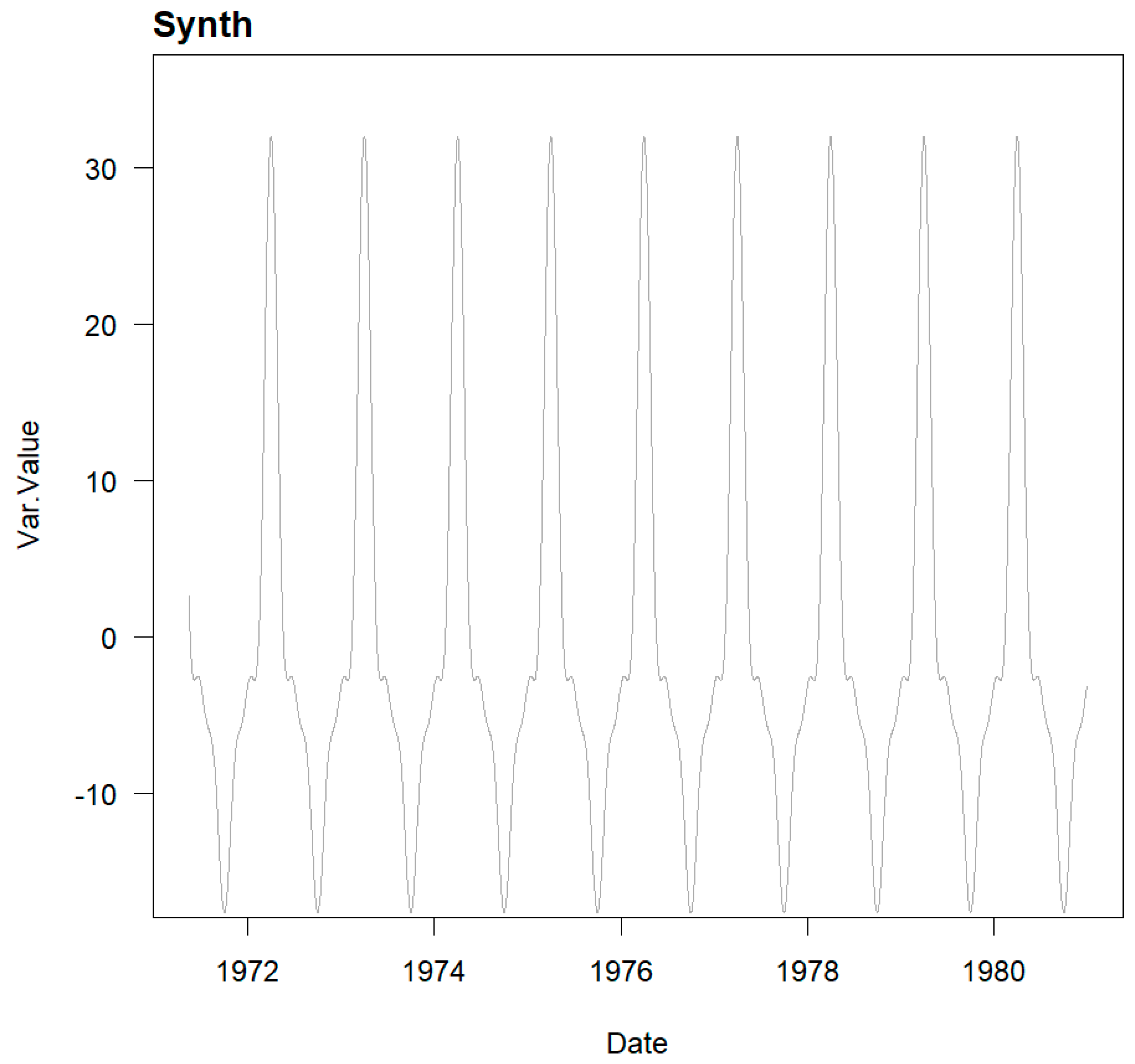
The pure synthetic stationary series obtained show the data Statistics and appearance as shown in
Table 1 and
Figure 2 below:
3.1.2. Behaviour-Based Stationary Series
The behaviour of monitored variables in dams, while exhibiting seasonal components and oscillatory characteristics, deviates from pure synthetic stationary series as it responds to a much more complex system. Therefore, the development of synthetic series that, while stationary, captures this behaviour is proposed in order to assess the ability of ML models to identify trends.
To obtain this kind of series, we started with the HTT model trained on a data set of n real data points from the radial movement of a direct pendulum in an arch dam, using the same expression as used to create the pure synthetic series.
This HTT model incorporates two time-dependent terms . By setting the calibrated polynomial coefficients a11 and a12 to zero, the series of predicted movement without considering the temporal effect will be obtained.
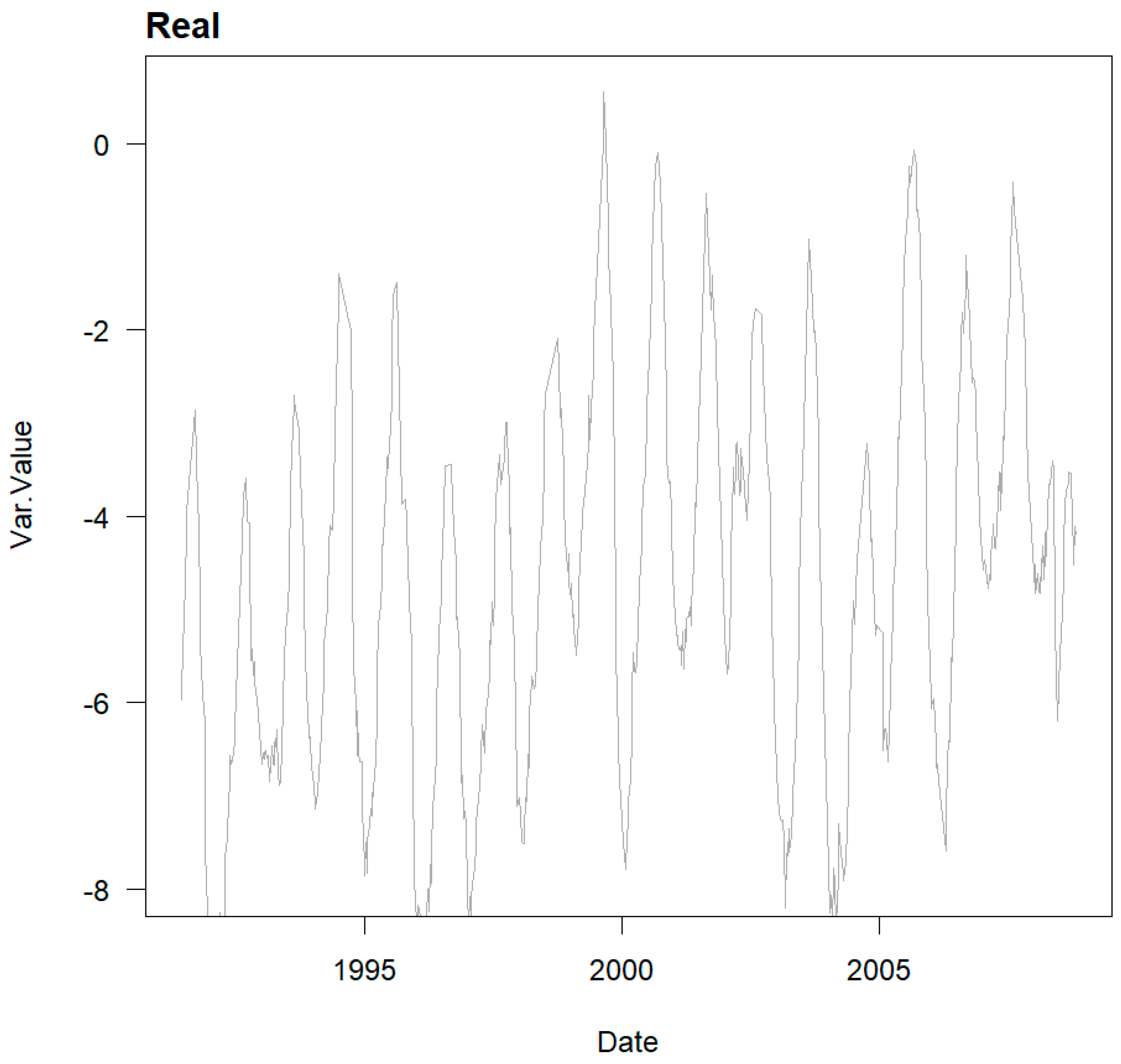
The behaviour-based stationary series obtained show the data Statistics and appearance as shown in
Table 2 and
Figure 3 below:
3.2. Generation of Trend Series
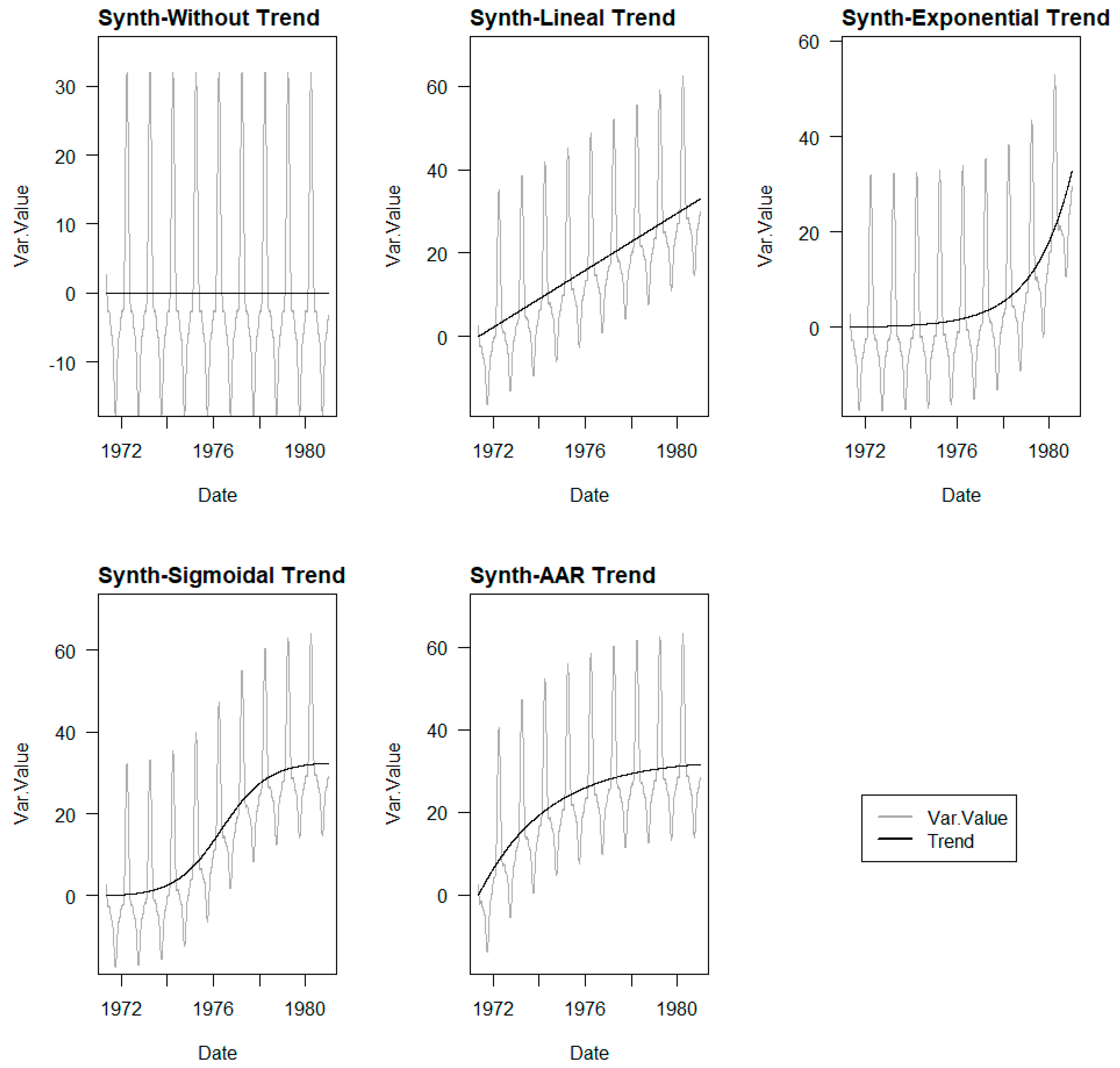
With the aim of evaluating the generality of the methodology, the use of different trend laws was proposed: linear, exponential, sigmoidal, and expansive reaction in concrete. These types of law are the most common in the movements recorded in dams. Depending on the process that governs these drifts and their degree of development, different types of trends can be encountered.
Geotechnical instability of the foundation can lead to linear creep phenomena over very long periods of time or to faster collapse phenomena in which the deformation rate increases exponentially over time. Other processes, such as expansive reactions in concrete, exhibit a slow onset in their development, which increases until a maximum expansion rate is reached and then gradually decreases until they practically stop. Thus, they respond to sigmoidal functions. Depending on the start point of the dam movement records, the data period, and the reactivity of the process, observations will generally cover a portion of these functions. Two sigmoidal formulations are used: a generic formulation in which the complete form of the function is developed, and another, proposed by Araujo (2005) [
32] for the characterisation of residual movements observed on the crest of dams affected by internal reactions, which is introduced only for decreasing slope ranges.
Consequently, the corresponding series of n records was constructed according to the following formulations:
Linear Trend: , where Ti is the time variable, m is the slope of the line, and kl is the y-intercept.
Exponential Trend: , where Ti is the time variable, d is the amplification parameter, p is the parameter associated with the growth rate of the trend, and ke is the y-intercept.
Sigmoidal Trend: , where Ti is the time variable, q is the parameter controlling the total increment in the y-axis, k1 is the parameter defining the time position of the inflection point of the function, k2 is the parameter defining the slope at the inflection point, and ks is the y-intercept at time zero.
Expansive Reaction Trend: , where Ti is the time variable, ka is the value of the y-intercept, B is the value of the y-intercept corresponding to the maximum increment, C is the time of the inflection point, and p is the parameter influencing the shape of the curve.
3.3. Generation of Experiments
Using the defined stationary series and trends, a battery of experiments is generated by their combination to evaluate the ability of ML models to identify trends in the series.
Thus, the experiments are divided into two main groups to be developed in Phase I and Phase II, based on the pure synthetic series and the stationary behaviour series, respectively.
Each type of base series is combined with the different trends, resulting in four series in each phase, to which the base series without trend of each type is added. In total, five series compose each of the two phases.
3.4. Development of Prediction Models
For each series, four types of prediction model are trained: SVM, BRT, NN, and HTT, resulting in a total of 20 experiments per phase, 40 experiments in total.
To avoid overfitting of the models during calibration, the cross-validation (CV) method was used. With this method, the training data set is divided into a series of n folds and n models are trained, each using one of the folds for training and the remaining fold for validation.
The division of the folds can be performed randomly or by sequential blocks. In this case, the latter strategy was employed, which is more suitable for modelling the behaviour of dams because, in time series where various regressors are involved, random division may provide the model with information from neighbouring records that could influence its interpretation.
Thus, in this research, one fold was taken for each year of data in the series.
To select the hyperparameters of each model, a brute-force algorithm or a grid search was employed.
The hyperparameters tuned by grid-search in each ML model were the following:
SVM;
- ○
sigma ∈ 0.001, 0.01, 0.1, 0.5, 1.
- ○
cost ∈ 1, 20, 50, 100, 200, 500, 1000.
BRT;
- ○
interaction depth ∈ 2, 3, 4, 5, 6, 7, 8.
- ○
N_trees ∈ 500, 1000, 2000, 5000.
- ○
Shrinkage ∈ 0.01, 0.001.
- ○
Nmin obs in node ∈ 5, 10, 15.
NN;
- ○
.
- ○
.
The parameters of the terms used for the HTT model were tuned by least squares.
3.5. Extraction of ML Trends
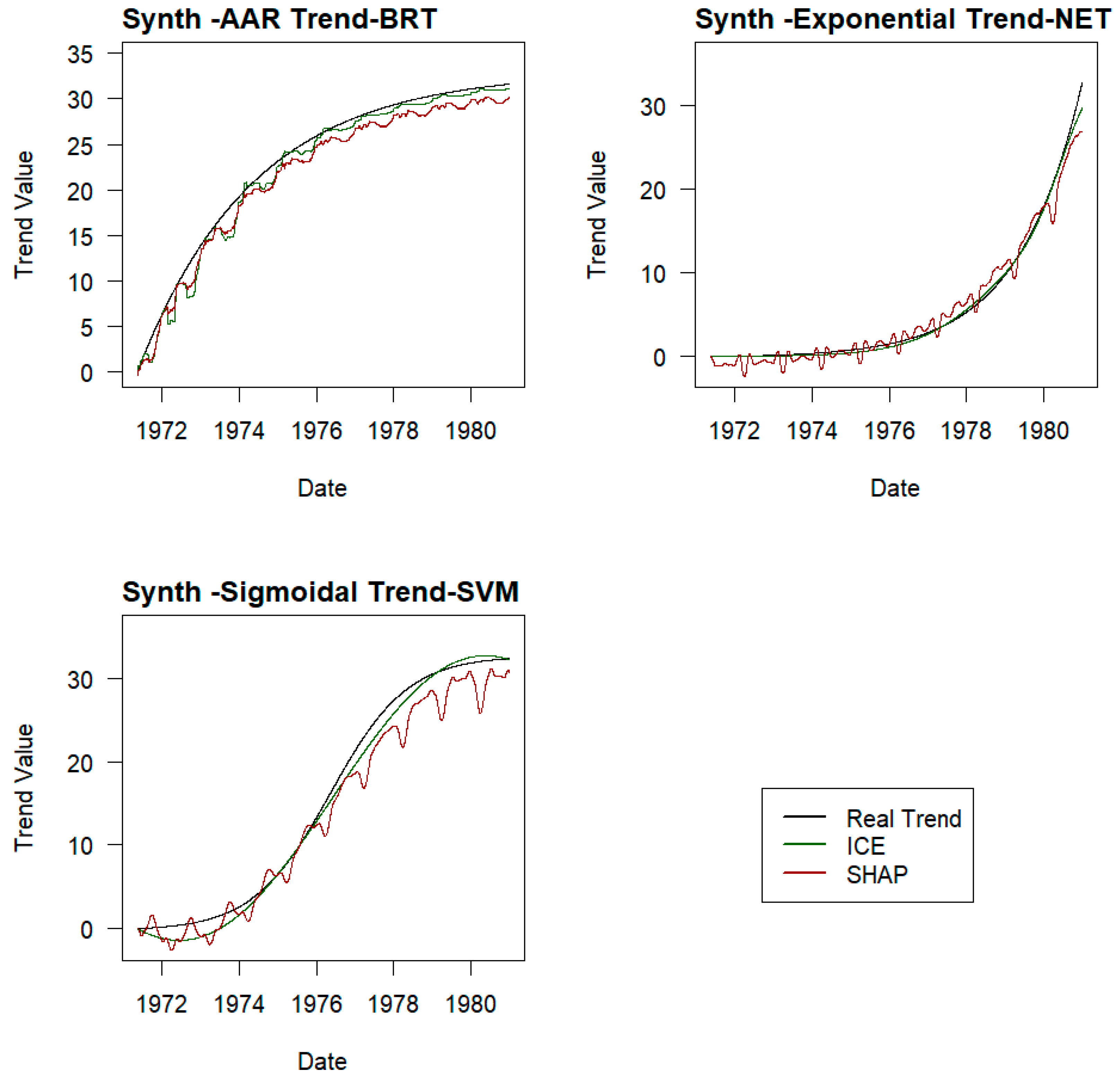
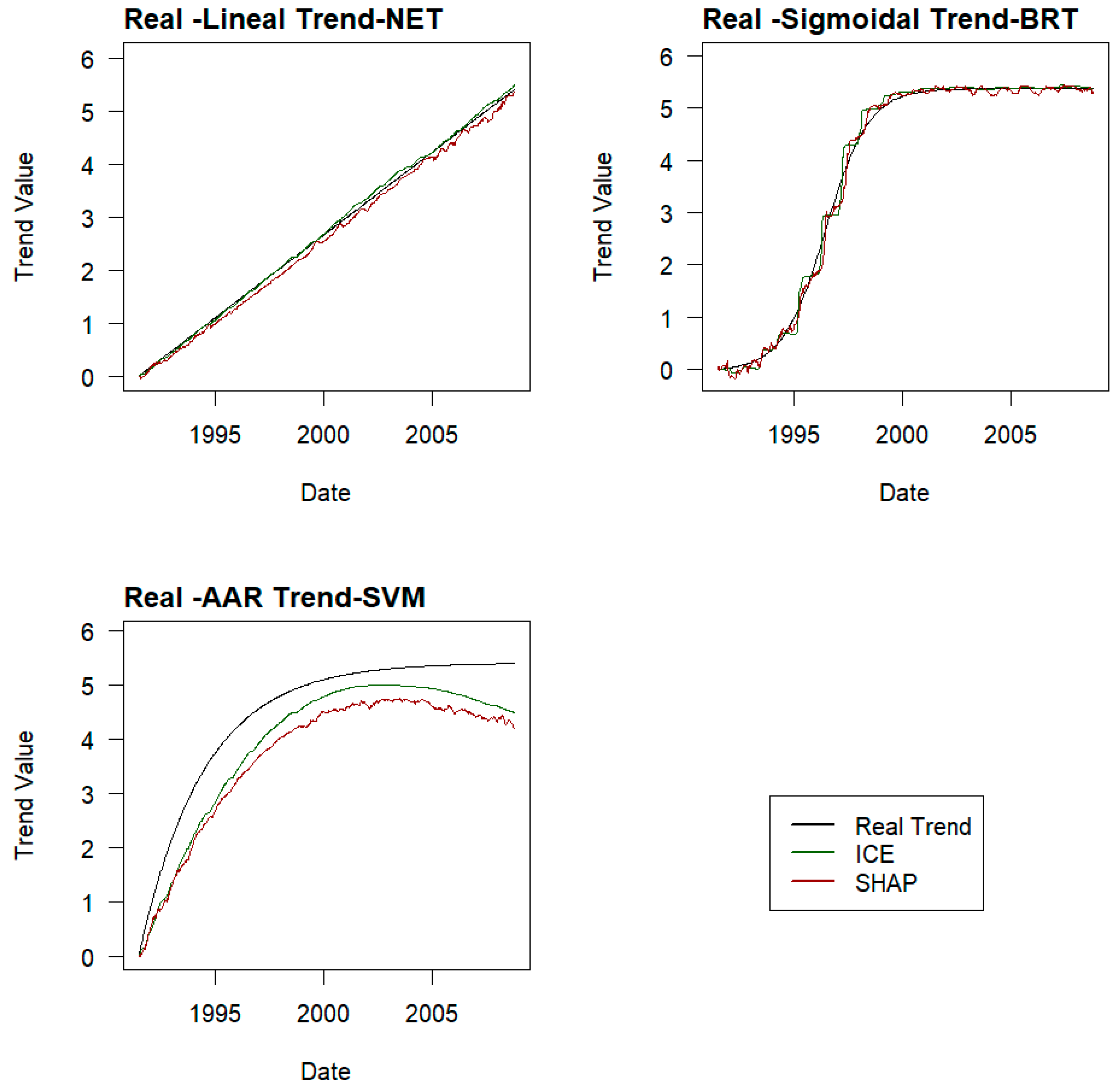
The hypothesis is that the ICE curve with “time” as the mobile explanatory variable, or the SHAP values corresponding to this variable, provides the part of the behaviour captured in the target variable that cannot be explained through the remaining explanatory variables, namely, the part that depends solely on time, the trend.
The determination of the trend based on the ICE curves relative to time in the different models is carried out following the following process.
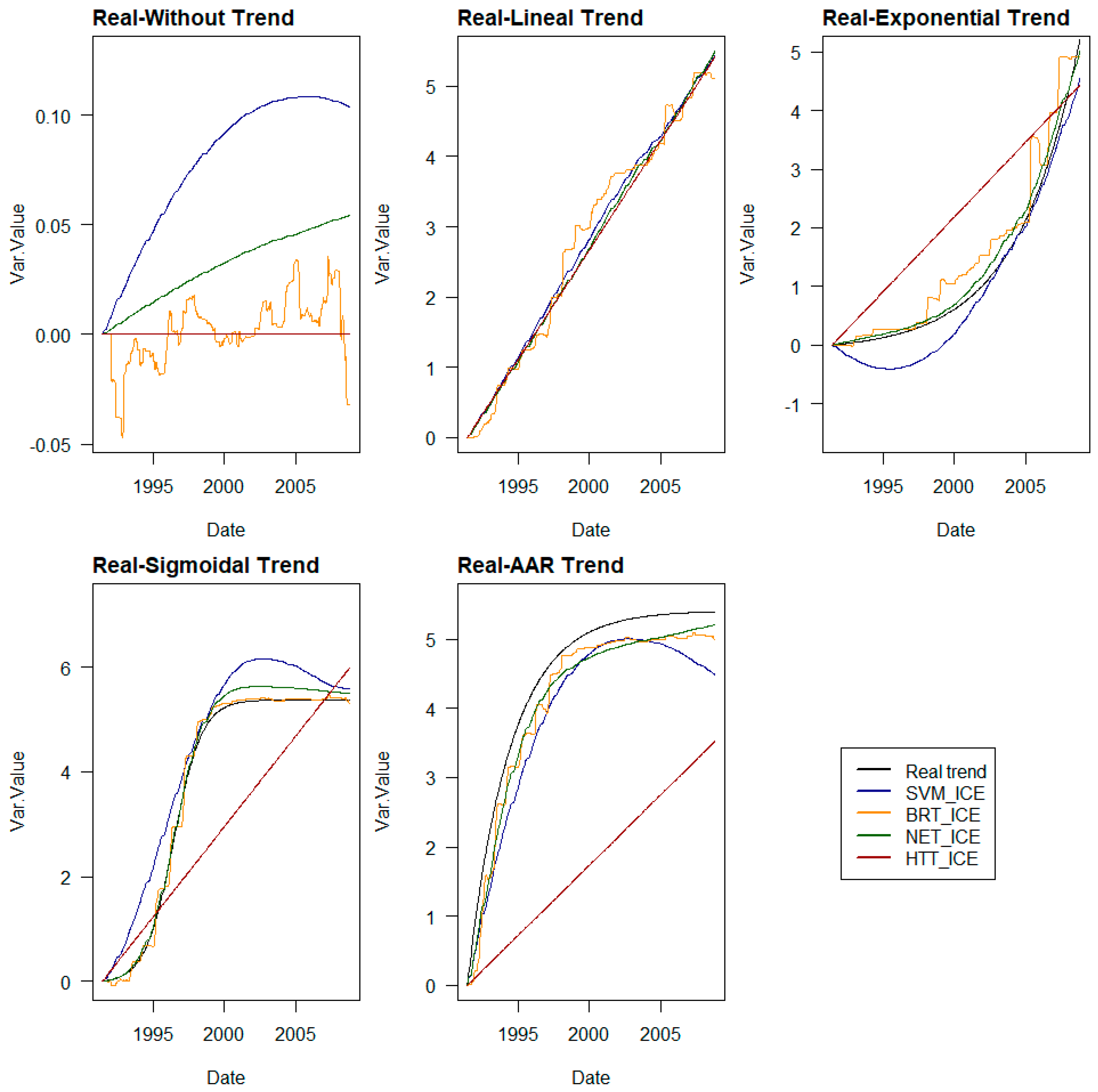
For each record in the dataset, the target variable is predicted with the trained models, while keeping all explanatory variables constant, except for the time variable, which varies throughout its domain in the data set. This provides a set of as many curves as there are records in the dataset, reflecting the variation of the model’s response when only the time variable changes, while keeping the values of the remaining variables fixed for each record.
For each value of the time variable in the dataset, the average value of the values obtained for that instant in the set of ICE curves is obtained.
The hypothetical trend curve is defined by these averaged values.
In this study, there are strong correlations between explanatory variables, since integrations of level or temperature are used over different time periods. However, the time variable does not show this strong correlation with any of them, and the combinations of values of strongly correlated variables are not altered in the process, making the method of ICE curves applicable. In any case, any doubts are dispelled by observing the procedure’s capability obtained from the test campaign conducted, beyond any theoretical discussion.
SHAP values corresponding to the variable ‘time’ are obtained following this process:
For each instance in the dataset, SHAP values are calculated by performing the following actions:
- ○
Evaluating the prediction of the model when the ‘time’ variable is included (active) and when it is excluded (inactive).
- ○
Compare these predictions to determine the impact of the feature.
- ○
Considering all possible combinations of features to ensure fair attribution.
The SHAP values for the variable ‘time’ represent the average marginal contribution of this feature across all possible combinations of features.
Trends are determined by both methods on a sample of three experiments in each phase. The RMSE, MAE, and R2 values of the trends obtained are compared with the real ones, and the method that provides the best result is selected.
The trends for the remaining experiments in each phase are determined using the selected method.
3.6. Adjustment of ML Trend Laws
The trends obtained with each model will be different from each other and will respond to the nature of each model’s algorithm and the relationships found between the explanatory variables and the target variable. While SVMs, by adjusting hyperplanes, or the employed neural networks (perceptron) provide smoother curves, BRT, being based on decision trees, provides stepped lines.
Adjusting these trend lines to the expected, or more common, trends in dam behaviour described in
Section 3.2 is carried out with the following coefficients as the variables to be adjusted:
Linear Trend: Coef.: m, kl
Exponential Trend: Coef.: d, p, ke
Sigmoidal Trend: Coef.: q, k1, k2, ks
Expansive Reaction Trend: Coef.: B, p, C, ka
Adjustment of the trend lines to these laws is carried out using the Grey Wolf Optimiser (GWO) algorithm [
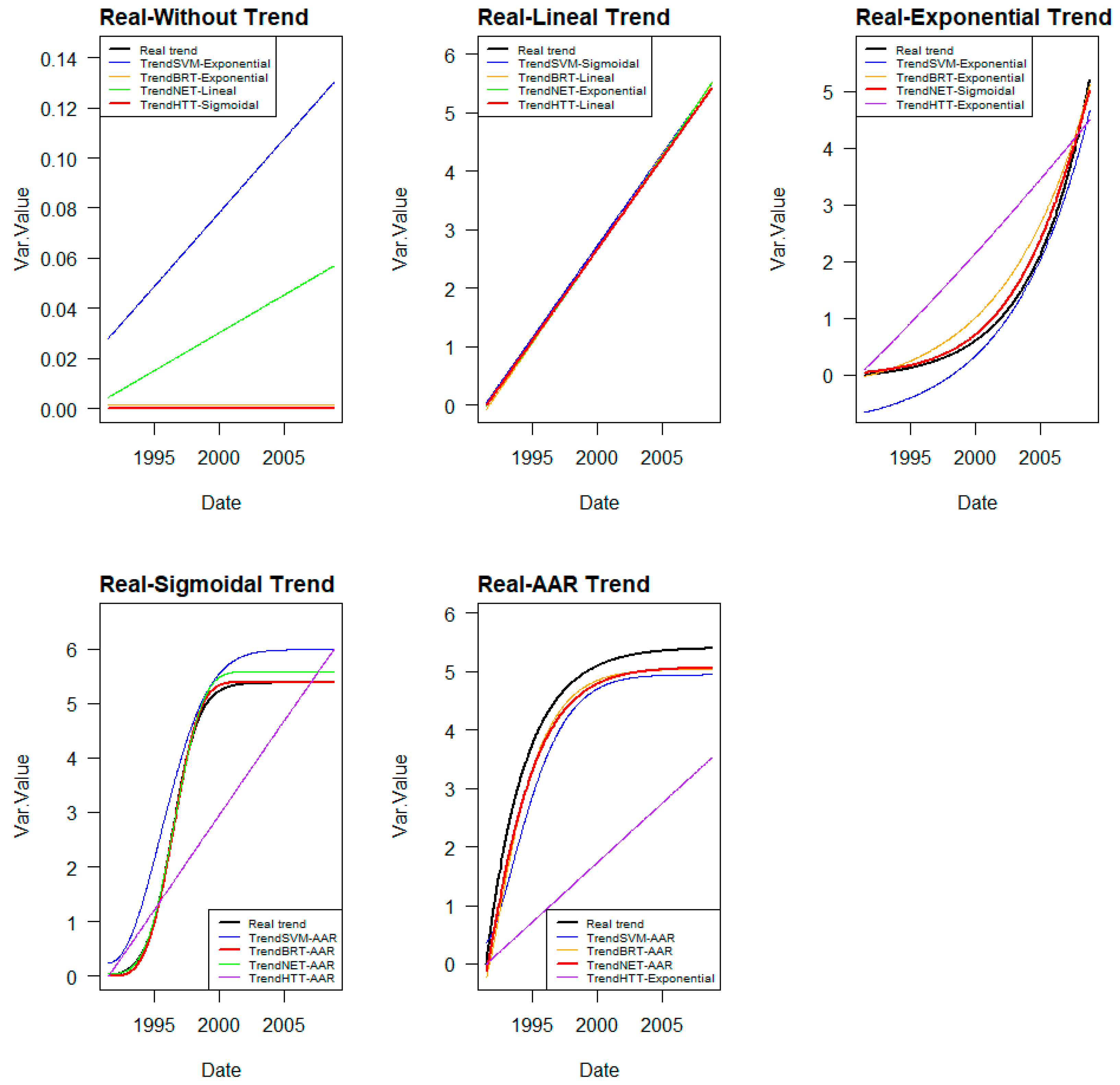
33]. For each trend extracted from the ML models, the four laws are fitted, and the RMSE, MAE, and R
2 of each fit are measured. The trend with the lowest errors and better performance is selected as the most plausible. The correctness of the trend selection is analysed.
3.7. Determining Error in Real Trends
Once the type of law that best fits each trend line extracted from the different ML models is selected, they are compared with the real trends introduced in the base series, measuring RMSE, MAE, and R
2.
where
represents the predicted values,
represents the mean of the actual values,
yi represents the i
th actual value, and
n is the number of records in the sample.

