Greedy Weighted Stacking of Machine Learning Models for Optimizing Dam Deformation Prediction

Abstract

Dam safety monitoring is critical due to its social, environmental, and economic implications. Although conventional statistical approaches have been used for surveillance, advancements in technology, particularly in Artificial Intelligence (AI) and Machine Learning (ML), offer promising avenues for enhancing predictive capabilities. We investigate the application of ML algorithms, including Boosted Regression Trees (BRT), Random Forest (RF), and Neural Networks (NN), focussing on their combination by Stacking to improve prediction accuracy on concrete dam deformation using radial displacement data from three dams. The methodology involves training first-level models (experts) using those algorithms, and a second-level meta-learner that combines their predictions using BRT, a Linear Model (LM) and the Greedy Weighted Algorithm (GWA). A comparative analysis demonstrates the superiority of Stacking over traditional methods. The GWA emerged as the most suitable meta-learner, enhancing the optimal expert in all cases, with improvement rates reaching up to 16.12% over the optimal expert. Our study addresses critical questions regarding the GWA’s expert weighting and its impact on prediction precision. The results indicate that the combination of accurate experts using the GWA improves model reliability by reducing error dispersion. However, variations in optimal weights over time necessitate robust error estimation using cross-validation by blocks. Furthermore, the assignment of weights to experts closely correlates with their precision: the more accurate a model is, the more weight that is assigned to it. The GWA improves on the optimal expert in most cases, including at extreme values of error, with improvement rates up to 41.74%. Our findings suggest that the proposed methodology significantly advances AI applications in infrastructure monitoring, with implications for dam safety.

1. Introduction and Background

Monitoring dam behaviour has maintained a transcendental significance role, given the significant social, environmental, and economic implications that its deterioration and failure could entail. Throughout time, conventional statistical approaches have served as surveillance systems, affording operators the requisite capabilities to identify irregularities and anomalies.

The advancement of technology and engineering has led to the creation of devices proficient in accumulating substantial volumes of monitoring data, thus instigating emerging requirements in the domain of dam safety.

The growing evolution of artificial intelligence, specifically within the domain of Machine Learning, introduces novel techniques that address these requirements in a comprehensive way [1]. Through Machine Learning, the development of accurate and robust predictive models is achievable. The applications of Machine Learning span diverse domains, encompassing even the intricate field of dam safety. Within this context, these models demonstrate significant efficacy in foreseeing dam behaviour, relying on their ability to integrate external conditions and past records. Such predictions, when quantitatively compared with empirical data, facilitate the determination of emergency thresholds based on observed disparities [2]. Thus, the imperative to maximise precision gains notable relevance.

The first-level models used in this research have different natures and have proven to be robust and accurate in making predictions in different domains.

Boosting Regression Trees (BRT) and Random Forest (RF) are Machine Learning algorithms based on decision trees for making predictions. While BRT constructs multiple trees sequentially, focussing on correcting errors in the previous model, RF constructs trees independently and averages their predictions to reduce variance [3]. Both algorithms are known for their ability to handle complex relationships in data and are commonly used in regression and classification problems. However, BRT may be prone to overfitting if not properly tuned, while RF may suffer from increased computational complexity with a large number of trees.

On the other hand, Neural Networks (NNs) are deep learning models inspired by the human brain. Composed of multiple layers of interconnected neurones, neural networks are capable of capturing complex and nonlinear relationships in data [4,5]. Although powerful, neural networks require large amounts of training data and hyperparameter tuning.

In the field of dam engineering, the Hydrostatic–Season–Time (HST) model has been extensively employed to assess dam safety by leveraging the impact of temperature through sinusoidal harmonic functions. However, despite its simplicity and interpretability, this methodology does not account for other external factors that can influence dam behaviour [6,7,8].

To address this limitation, several researchers have turned to Machine Learning techniques, whose algorithms enable the modelling of dam behaviour based on external conditions and historical trends. In this context, Fernando Salazar has frequently utilised ensemble decision tree algorithms in various studies, producing excellent results [9,10,11]. They compare ML models with conventional statistical models, and they concluded that BRT outperforms the alternatives, followed by RF and NNs [9]. They also demonstrate that BRT not only serves to make robust predictions, but also serves as a tool for the interpretation. The behaviour of dams can be seen as a function of environmental factors through the predictive importance of the variables that the BRT can generate [11]. Furthermore, they propose a method for anomaly detection by training a BRT model and setting a criterion based on its residual density function [2].

Another widely used algorithm is Support Vector Machines (SVMs). Ranković et al. successfully predicted the tangential displacement of a concrete dam using an SVM model [12]. Furthermore, they concluded that this model is significantly influenced by the hyperparameters used in its training process. Mohammad Amin Hariri-Ardebili also adopts the Support Vector Machine (SVM) approach and presents two extensive applications: one for a simplified assessment of the reliability of gravity dams and another for a detailed nonlinear seismic analysis based on the finite element method (FEM), confirming the accuracy of SVMs for these kinds of issue [5,13].

Mata compares a multiple linear regression with NNs, concluding that NNs represent a flexible and robust approach to predicting dam displacement, particularly under extreme temperature conditions [13]. On the other hand, in [14], a novel approach utilizing deep neural networks and optimization algorithms to identify the soil parameters for the accurate modelling of rockfill dams is described. The methodology, applied to a dam in Quebec, involves numerical solutions and inverse analysis using surrogate models. Comparative studies assess material heterogeneity, while stochastic optimization algorithms are evaluated for parameter minimization, demonstrating the effectiveness of the proposed approach [14].

In research practice, investigators commonly employ these algorithms by simulating a standard regression problem, where external conditions and historical information serve as explanatory variables, and the device’s series functions as the target variable. However, this issue can be approached from a time series perspective, as monitoring data follows a temporal structure. Among the most prominent approaches in recent years for time series prediction are Long Short-Term Memory (LSTM) neural networks, which address the memory limitations of conventional neural networks and outperform traditional methods such as ARIMA [15,16].

After reviewing the existing literature, it becomes evident that methods such as BRT, RF, NN, and HST models are widely utilized in various domains and have consistently demonstrated a robust and reliable performance. These methods exhibit diverse characteristics, with BRT and RF being ensemble methods based on decision trees, while NNs and HST represent different modelling approaches. Given their reliability and track record of delivering favourable results, we selected them as experts in our research. However, we acknowledge that algorithms such as LSTM and SVM also yield excellent results. Hence, our intention for future investigations is to broaden the pool of experts by incorporating additional algorithms and optimization strategies.

When models are trained across a range of the aforementioned methods, it becomes evident that disparate models exhibit distinct error patterns. The possibility arises that the optimal model, denoted as “expert” within the context of our study, might not remain consistent over the entirety of the time series.

Combining BRT, NN, RF, and HST models offers a synergistic approach to addressing their individual limitations and capitalize on their complementary strengths. BRT, while powerful, may struggle with overfitting and sensitivity to outliers. Neural Networks, renowned for their ability to capture complex patterns, may face challenges such as the need for large amounts of data to train effectively, susceptibility to vanishing or exploding gradients, and difficulty in providing interpretable results. RFs, known for their robustness, might lack sensitivity to subtle relationships in the data. HST models, although effective for capturing seasonal variations, may overlook spatial dependencies. By integrating these models via ML techniques, we mitigate these shortcomings, harnessing the collective predictive prowess to achieve more accurate and resilient dam deformation predictions.

This realisation underscores the fundamental objective of our research: the orchestration of expert model combination to meticulously enhance precision through the strategic application of Stacking.

The Stacking technique, recognised as stacked generalisation, was originally formulated by Wolpert in 1992. In essence, this methodology revolves around the training of a second-level model, denoted as meta-learner, using the prediction vectors produced by experts obtained through the Cross-Validation procedure [17]. In an illuminating study, Zeroski substantiates the efficacy of this approach, leveraging a comprehensive array of 30 open-source datasets. Empirical evidence underscores that a meta-learner adopting the multiple linear regression or decision tree paradigm excels beyond the strategy of exclusively selecting the most accurate expert model [18].

Wu et al. employ bagging, boosting, and stacking techniques to combine classifiers and improve the accuracy of daily reference evapotranspiration estimates. Their results suggest that all models are suitable for landslide modelling, although the SVM boost model exhibited a higher predictive accuracy [19]. In a similar vein, Dou et al. adopted the same strategy to predict the assessment of landslides. In their case, the SVM boost model outperformed the other models, while the SVM stacking model yielded the lowest performance [20].

Within the domain of dam safety, the literature offers limited instances where the combination of first-level models through the Stacking technique is explored. Some researchers apply Stacking for the purpose of a multitarget prediction [21,22], while others attempt to reveal discernible patterns in model behaviour to delineate the threshold criteria governing the selection of one model over another [23]. Furthermore, certain authors harness predictions derived from statistical and time series models as inputs for a second-level model, meticulously trained using the principles of Extreme Machine Learning [24]. In particular, Lei W. and Wang J. utilize a Stacking ensemble meta-learner to forecast dam displacement, highlighting its superior precision and robustness compared to expert opinions. Their approach incorporates feature selection with PCA-RF, Bayesian optimisation for hyperparameter tuning, and dynamic monitoring indexes, resulting in enhanced accuracy and reliability for the dynamic safety warning of dam deformation [25].

In our paper titled “Prediction of Concrete Dam Deformation through the Combination of Machine Learning Models”, we trained second-level predictive models using Stacking and Blending techniques on radial displacement data from an arch-gravity dam, employing Generalized Linear Regression (GLM). Our findings underscore that the Stacking approach achieves higher precision than first-level models in most scenarios [26].

The majority of Stacking meta-learners are rooted in linear models. Within our research inquiry, we undertake a comparative analysis of diverse algorithms, varying in levels of complexity, to discern the optimal mode of expert combination. Among these algorithms, the Greedy Weighted Algorithm (GWA) has emerged as a particularly effective contender in the domain of Stacking. A case in point is the study by Kurz et al., where a greedy algorithm is implemented across a spectrum of seven data sets that span multifaceted biomedical disciplines, consistently exceeding the performance of the linear model in numerous scenarios [27]. The intricate details of this algorithm are elucidated for the reader in a subsequent section to facilitate the understanding of the research. In our study, we chose this algorithm along with a linear model and BRT to combine experts and determine the most effective approach to improve the precision of the leading expert.

This research stands out for its innovative nature and relevance, as there is limited research into expert combinations in the field of dam safety. To our knowledge, there are no existing articles that compare various meta-learner construction methods in this specific domain.

The structure of the article commences with the introduction, followed by a dedicated section detailing the Greedy Weighted Algorithm (GWA). We have segregated this section because we believe it holds particular significance within the research, being the integrator that yields the best results. Therefore, we aim for its functioning to be well comprehended. Subsequently, we have the sections “General approach”, which succinctly summarises the methodology, serving as a guide for the reader to navigate through the research, and “Dam Cases”, where the data are described. Next, we delve into the core methodology and results, divided into two sections: “Predictive modelling with meta-learners” and “Three questions about weight estimation”. Within each, we have included two subsections: methodology and results. Finally, we conclude with the conclusions section.

2. Greedy Weighted Algorithm

Among the algorithms used for the combination of models, the Greedy Weighted Algorithm (GWA) [27] deserves a more comprehensive explanation due to its optimal meta-learner properties, as elucidated in forthcoming sections.

The GWA operates as a weight-assignment model, where the ultimate prediction of the response variable is a combination of previously trained experts, following the mathematical formulation:

$$\widehat{y}=\sum _{i=1}^k{\beta }_i\ast p_i;$$

(1)

where $k$ represents the total number of experts, ${\beta }_i$ denotes the weight assigned to expert i, and $p_i$ corresponds to the prediction vector of the same expert.

The algorithm iteratively assigns weights to different experts, with the aim of building combinations by selecting the one exhibiting the lowest error. In the initial iteration, no combinations are formed; rather, the expert with the lowest Root-Mean-Square Error (RMSE) is chosen. Subsequently, in each iteration, an increased weight is assigned to the selected expert. This process continues, ultimately determining the final weight for each expert. The final weight of an expert results from a voting procedure, in which the number of times an expert achieved the lowest error is counted and divided by the total number of votes, which is equal to the number of defined iterations [27].

Algorithm 1 outlines the steps involved. However, before delving into the algorithm, it is necessary to define the elements associated with its execution:

Algorithm 1: The greedy weighting algorithm [27]

$X \left(mxk\right)$: A matrix containing the predictions of experts, where m is the number of rows and k is the number of experts. $Y$: A vector representing the response variable. $weights$: A vector initialised with zeros containing the weights for each expert. The number of entries corresponds to the number of experts. $Z \left(mxk\right)$: A zero initialised matrix that holds the updated prediction vectors based on the assigned weights. $s$: A parameter controlling the number of iterations, determining the total number of times the weights are updated. $e$: A vector of RMSEs for each expert. The number of entries matches the number of experts. Result: $\mathrm{Vector} w$ with the weights of each expert.   1. $\mathrm{Initialize} weights$ to a vector of 0.   2. $\mathrm{Initialize} Z$ to a matrix of 0.   3. $\mathrm{Initialize} s$ to 0.   4. WHILE $(s<iter$) DO: $s=s+1;$ $Z=\left(Z+X\right)\ast \raisebox{1ex}{$1$}\!\left/ \!\raisebox{-1ex}{$s$}\right.;$ $e=RMSE\left(Z,Y\right);$ $best=which\left[\min \left(e\right)\right];$ $Z=Z\left[,best\right]\ast s;$   5. END WHILE   6. $w=\raisebox{1ex}{$weights$}\!\left/ \!\raisebox{-1ex}{$s$}\right.$

To provide a more detailed description of the Algorithm 1 and facilitate its interpretation, presented here is an example illustrating the combination of three experts: BRT, NN, and HST, over five iterations.

• During the initial iteration, the algorithm identifies the expert with the lowest error as the selected candidate.
• In the subsequent iteration, the algorithm combines the previous optimal solution with each expert by assigning them a weight of 1/2. For example, if BRT is determined as the best expert, the expression for the HST column would be 1/2BRT + 1/2HST. Consequently, each expert represents a combination of itself with the optimal expert identified above. Subsequently, the error of each combination is computed and the combination with the lowest Root-Mean-Square Error (RMSE) is chosen. The selected combination is then multiplied by the total number of weights (in this case, 2), resulting in a new vector representation. For example, if HST is the optimal expert, the updated vector would be (1/2BRT + 1/2HST) × 2 = BRT + HST.
• In the subsequent iteration, the algorithm augments the previous vector, BRT + HST, by combining it with each expert while assigning a weight of 1/3 to each. Thus, for NNs, the resulting combination would be 1/3BRT + 1/3HST + 1/3NN, and the same principle applies to the remaining experts. Following this, the error of each combination is calculated, and the combination with the lowest RMSE is selected. The optimal combination is then multiplied by the total number of weights. Should the combination involving NNs yield the best result, the updated vector would be (1/3BRT + 1/3HST + 1/3NN) × 3 = BRT + HST + NN.
• The subsequent iteration involves adding the previous vector, BRT + HST + NN, to each expert while assigning a weight of 1/4 to each expert. For example, for BRT, the resulting combination would be 1/4BRT + 1/4HST + 1/4NN + 1/4BRT, and the same procedure applies to the remaining experts. Subsequently, the error of each combination is calculated, and the combination with the lowest error is selected. The optimal combination is then multiplied by the total number of weights. If the combination involving BRT is determined as the best, it can be expressed as (1/4BRT + 1/4HST + 1/4NN + 1/4BRT) × 4 = BRT + HST + NN + BRT = 2BRT + HST + NN.
• In the final iteration, the algorithm adds the previous vector, 2BRT + HST + NN, to each expert while assigning a weight of 1/5 to each. For example, for BRT, the resulting combination would be 2/5BRT + 1/5HST + 1/5NN + 1/5BRT, and the same procedure is applied to the remaining experts. Subsequently, the error of each combination is calculated, and the combination with the lowest error is selected. The optimal combination is then multiplied by the total number of weights. If the combination involving BRT is determined as the best, the resulting expression would be (2/5BRT + 1/5HST + 1/5NN + 1/5BRT) × 5 = 2BRT + HST + NN + BRT = 3BRT + HST + NN.

In the final weight counter vector, BRT accumulates three votes from iterations 1, 4, and 5, HST accumulates one vote from iteration 2, and the NN accumulates one vote from iteration 3. Ultimately, the total weight of each expert is determined by dividing the number of votes by the total number of iterations (votes). Thus, the final weights for each expert would be 3/5 for BRT, 1/5 for HST, and 1/5 for NN.

3. General Approach

This section presents a brief description of the structure of this research. The main objective is to develop a first-level model combination methodology that improves the accuracy of the optimal expert.

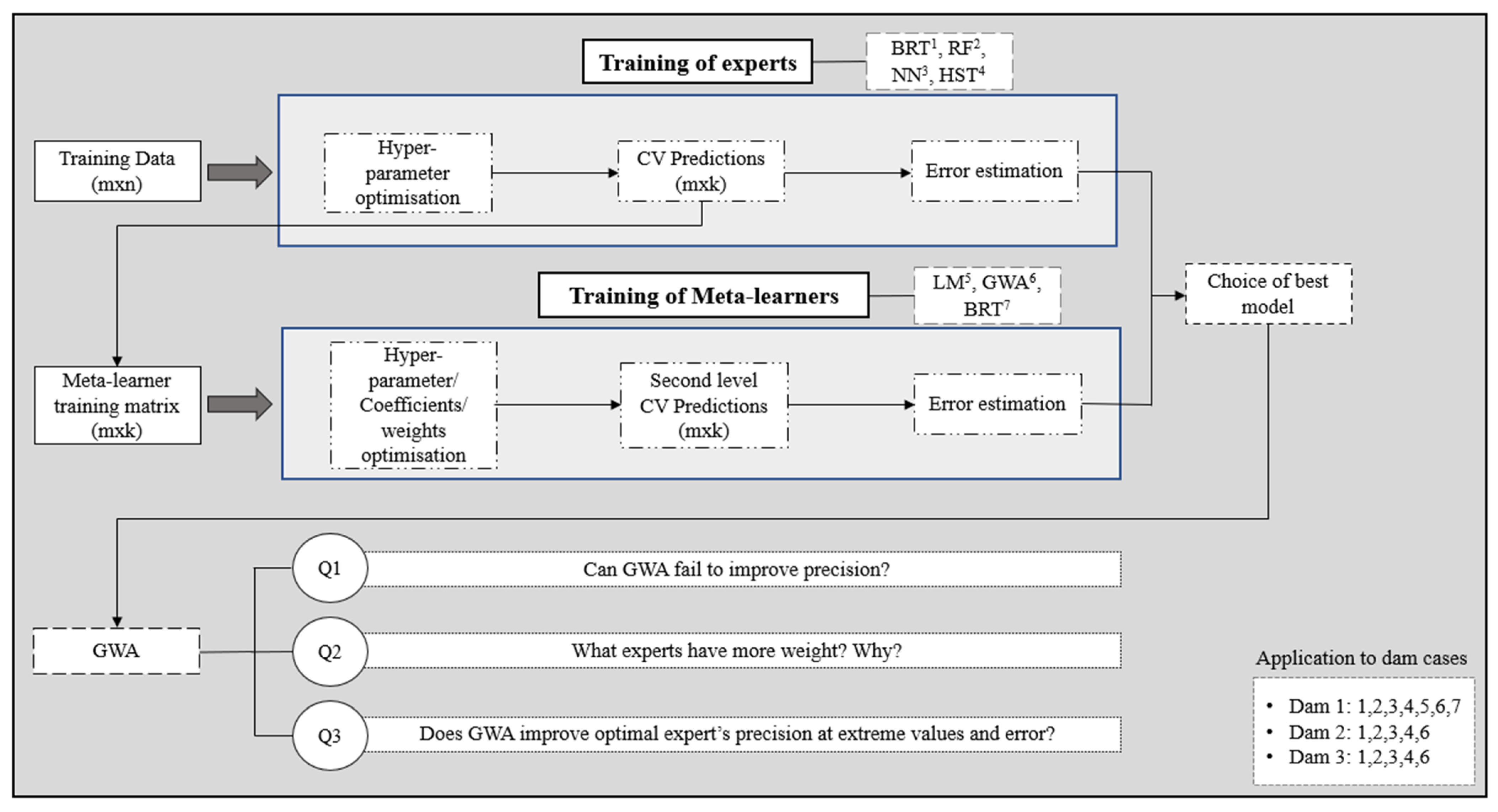
The structure of this paper has been divided into two fundamental parts (Figure 1): the training of experts and meta-learners, and a block of questions that arise when analysing the results of the optimal meta-learner (GWA).

First, the experts were trained with the m × n-dimensional training dataset. In order to cover possible predictive shortcomings of the experts and improve accuracy, algorithms of different natures were selected, such as ensembles of decision trees (BRT and RF), neural networks (NNs), and Hydrostatic–Seasonal–Time (HST).

The Blocked Cross Validation evaluation process was used, where each block equals one year. This provided a method to reach the optimal hyper-parameters and to obtain an estimate of the error in future data. Furthermore, the predictions of each block were obtained, which served as the input data set for the next stage of the research: the training of the meta-learners.

Algorithms of higher and lower complexity were chosen as second-level models: linear models, such as simple Linear Regression (LM) and the Greedy Weighted Algorithm (GWA), and decision tree ensembles (BRT). The predictions obtained during the Blocked CV at this stage were also used to make an error estimate, which was compared with the optimal expert’s error through their relative difference. Following this comparison, the best model was determined.

As will be seen in the analysis and discussion of the results, the best meta-learner was the GWA. At this point, three questions emerged regarding the performance of this algorithm and the increase in precision, which are directly linked to the weight estimation.

The first question arises intuitively, as it is an algorithm that gives weights to each first-level model: Can the GWA fail to improve precision? The reader might give a negative answer, as it seems reasonable to give a weight of 1 to the optimal expert and 0 to the rest in case their combination did not improve the accuracy. To solve this question, the optimal weights of each expert in each fold were calculated and compared with the weights given by the algorithm during the Blocked CV. This will be explained in detail in Section 5.1.

The second issue of concern was which experts had the most weight and why. Since the results already obtained were used to answer this question, the reader will not find a methodology explanation in this section. The response boils down to the comparison of the weights given and the estimated errors during the CV.

To conclude this part of the research, it was studied whether the second-level model improved the predictions of the optimal expert where it made the greatest error. To this end, we extracted errors that were lower than the limit of quartile one and higher than the limit of quartile three. Then, the errors of the expert and the meta-learner were calculated and compared at those values. Additionally, the same methodology was applied to the periods in which extreme values of radial displacement, water level, and temperature are found.

The proposed methodology was applied to three different dams, following a specific order that is relevant to mention. First, the experts and second-level models were trained on the pendulum series of dam 1. The algorithms used were BRT, LM, and GWA. Since the GWA was the best meta-learner, it was selected to train meta-learners on the data of dams 2 and 3. The experts trained on the series of these dams were the same as in the first case.

4. Dam Cases

This section presents the main characteristics of the dam cases, as well as the graphs of the series of the target variables and the external conditions. Data are available for three dams of different types: arch-gravity, gravity, and double curved arch dam, with heights ranging from 45 to 99 m above foundation,

Table 1. Summary of the dams whose data have been used during the research.

Dam	Type	Height	Target	Devices	Instances	Explanatory Variables	Date Range
Dam 1	Arch-gravity	>66 m	Radial movement	4 pendulums	3560	5	2004–2017
Dam 2	Gravity	99 m	Radial movement	2 pendulums	216	4	1992–2020
Dam 3	Double curved arch dam	45 m	Radial movement	2 pendulums	681	3	2000–2012

. The data sources are three different research projects on three different dams, two of them located in Spain and one in France. Due to confidentiality reasons, no details are given on the name of the dam or its exact location.

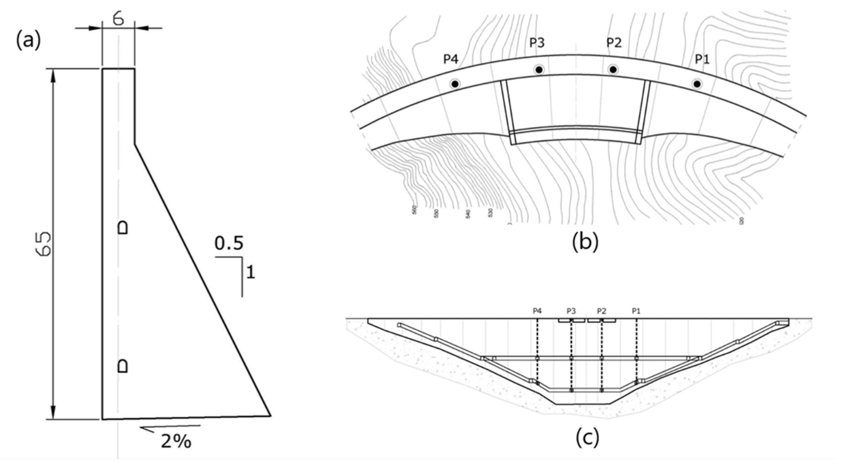
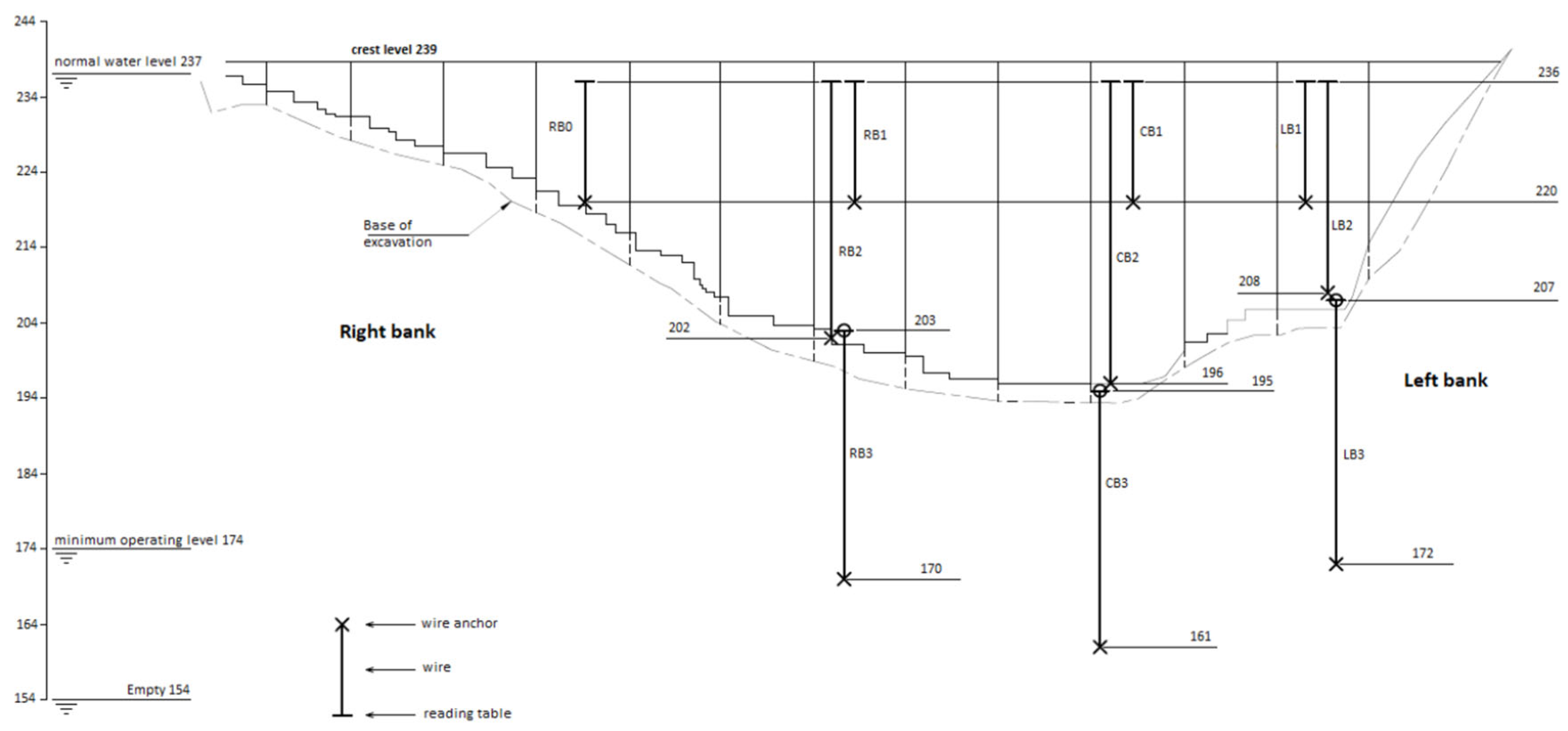
The dams are equipped with various monitoring devices that allow for control of the safety of the dam. Radial displacement of the structure is a reliable measure closely related to the safety of the dam. Therefore, auscultation devices were selected for this purpose for all dams. In the case of dam 1, four pendulums were used, placed in the upper zone and in the horizontal gallery (Figure 2). However, for the second dam, bisection movement sensors were selected at two points located in a downstream overhang close to the crest in the central blocks (Figure 3). The two selected pendulums from dam 3 are located in block CB in Figure 4.

To extrapolate the methodology’s efficacy comprehensively, it is imperative to explore its applicability with other sensors measuring different aspects of dam safety. Future investigations are planned to evaluate the methodology’s performance using diverse sensor types, aiming to provide a more holistic assessment of overall dam safety.

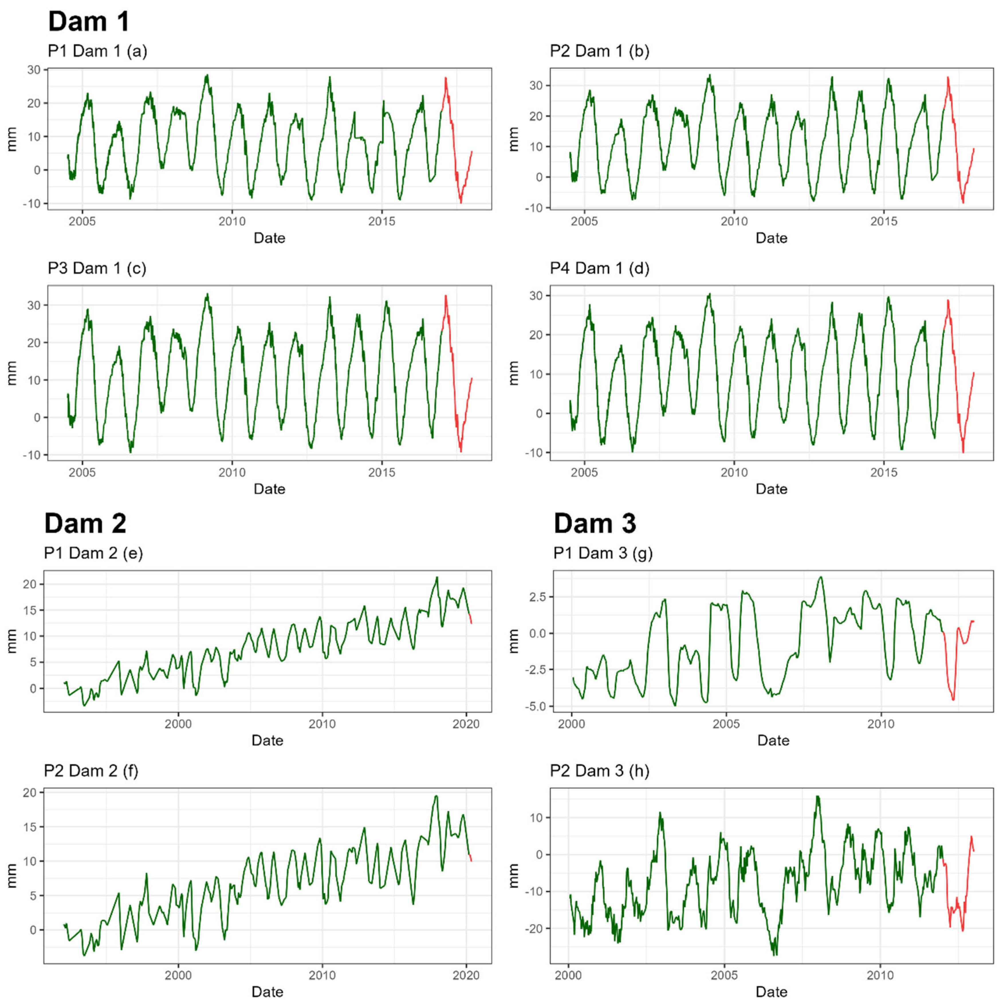
The highest number of available records corresponds to the first dam, with 3560 records, while the lowest number belongs to dam 2, with only 216 records (Table 1). The date ranges available differ depending on the dam, but in all cases the last available year is reserved for the last validation, in red in the figure (Figure 5). However, the errors used for the model comparison are the ones obtained during Cross Validation, as it is a more reliable estimate as it is an average over several years (

Table 2. Cross Validation by Blocks. The green colour represents training folds, while the blue colour represents test folds.

Year	Year1	Year2	…	Yearn
Iteration1
Iteration2
…	…	…	…	…
Iterationn

).

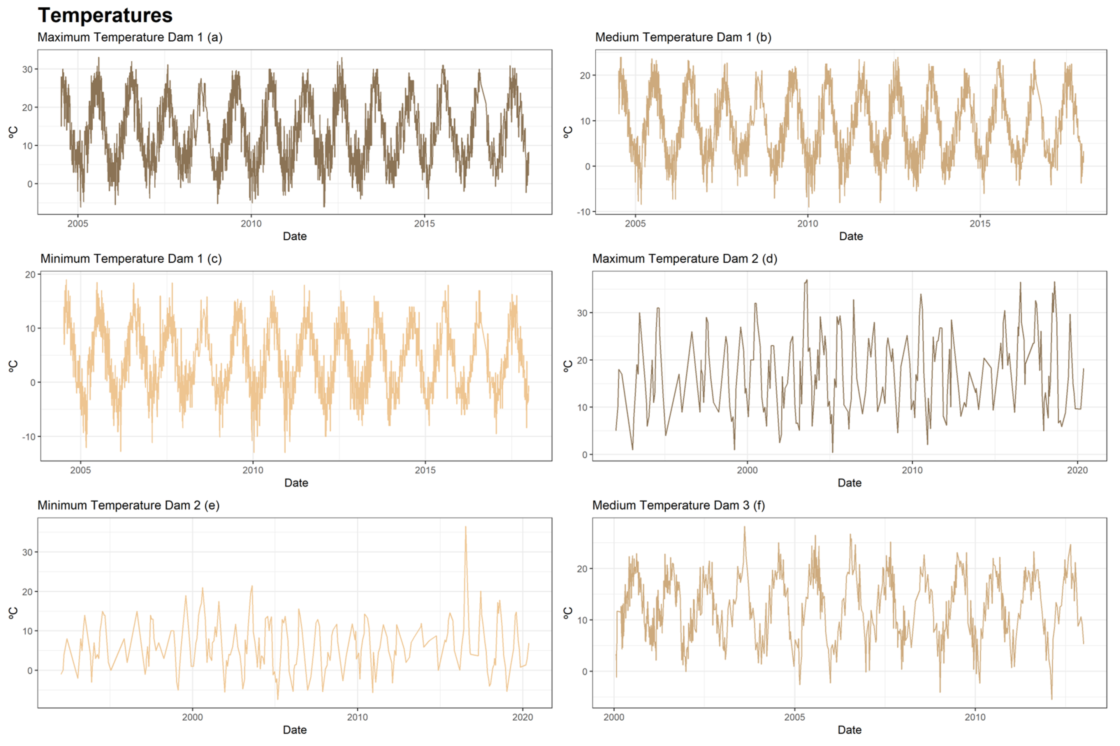
The external conditions that serve as explanatory variables for experts are rainfall (Figure 6), temperatures (Figure 7) and reservoir level (Figure 8). From these, synthetic variables related to the past were calculated for each of them. Moving averages, aggregates, and speeds of variation of different orders (7, 15, 30, 60, 90, 180, and 365 days) were calculated.

5. Predictive Modelling with Meta-Learners

This chapter addresses the training of experts and the development of second-level models. It is structured into two subsections: methodology, wherein the executed actions are elucidated, and results and discussion.

5.1. Methodology

The initial phase of the methodology included the selection of algorithms for expert training. Given the primary goal of enhancing the accuracy of the optimal expert, a diverse range of algorithms were chosen to mitigate their individual limitations through their combination. Each selected model demonstrates a significant level of quality, drawing from both established research and our own empirical insights. Consequently, ensembles of decision trees (specifically BRT and RF), Neural Networks (NNs), and Hydrostatic–Season–Time (HST) were selected.

The data sets used for expert training contain information about the external conditions of the dam. Moreover, to capture the influence of the past behaviour of these variables, moving averages, aggregates, and variation rates were calculated for each of them and added as synthetic variables.

On the other hand, the evaluation process used to reach the optimal hyperparameters and estimate the error on future data was Cross-Validation by blocks, where each block represents a year. Through this procedure, we obtained the prediction vectors of each expert, which shape the training matrix of the meta-learners:

“By joining these vectors to the target variable $Y={\left\{y_1,y_2,...,y_m\right\}}^T$, the following training matrix $[m\times (k+1\left)\right]$ is obtained:

$$D^{\prime }=\left(\begin{array}{cccc}{p}_{11}& \cdots & p_{1k}& y_1\\ ⋮& \ddots & ⋮& ⋮\\ p_{m1}& \cdots & p_{mk}& y_m\end{array}\right),$$

where $p_{ij}$ is prediction $i$ of the expert $j$. The first column in Equation (3) is the prediction vector of expert 1, $p_1\left(Y\right)=\left\{p_{11},p_{21},\dots ,p_{\mathrm{m}1}\right\},$ and so on.” [26].

Once the training set was configured, the meta-learners were trained. Three distinct algorithms of varying complexity were selected: simple linear regression (LM), greedy weight estimation (GWA), and an ensemble of decision trees (BRT). Given the limited number of variables in this new dataset, all of which exhibit linear relationships with the target variable, linear models were considered suitable. Specifically, the weight estimation algorithm was chosen to mitigate potential issues related to multicollinearity. Lastly, BRT was chosen for its predictive quality in standard problems.

An important aspect to be elaborated on is the estimation of the coefficients and weights assigned to the experts. The determination of hyper-parameters for the BRT meta-learner was executed through Blocked Cross Validation, mirroring the approach employed for the BRT expert. Conversely, in the case of the other two second-level models, Cross-Validation does not impact the estimation of final coefficients and weights; rather, it serves solely to estimate the error.

In summary, the challenge encountered in this phase of the research lies in the estimation of coefficients and weights for experts within the training set. The aim is to apply these estimates to the predictions generated by experts on the forthcoming data [27]:

$$\widehat{y}=\sum _{j=1}^k{w}_j{p}_j;$$

(2)

where $w_j$ is the vector of final weights or coefficients of expert $j$, $k$ the total number of experts, and $p_j$ the vector of predictions of expert $j$.

The weights were estimated considering the entirety of the data in matrix $D\prime$, referenced above. However, an error estimate is needed to ensure that the model is accurate and robust. At this point, the usefulness of the CV for the LM and GWA meta-learners arises.

Under the assumption of having have $n$ years available in the data set, the CV will comprise $n$ iterations, as each block represents a year. To estimate the error for the GWA and LM, within each iteration, we computed the weights and coefficients using all years (as indicated by the green entries in Table 2). The exception was one year designated as the test fold (in blue in Table 2). Therefore, for each year, we obtained a vector of weights estimated with the data for the remaining $n-1$ years. We believe that this assessment approach is close to reflecting the actual problem and, therefore, most suitable.

The weights estimated with each training subset were applied to the prediction vectors of the $D\prime$ matrix of the test fold, resulting in an associated error value. Hence, in addition to the vectors of weights and coefficients, we obtained $n$ error values. The selected error measure in this context is the Rooted-Mean-Squared Error (RMSE), a customary choice in machine learning problems:

$$RMSE=\sqrt{\sum _{i=1}^m\frac{{({\widehat{y}}_i-y_i)}^2}{m}};$$

(3)

where ${\widehat{y}}_i$ is the predicted value of $i$, $y_i$ is the observed value of $i$, and $m$ is the total number of records.

The ultimate estimated error is determined by computing the average of the errors observed across all test folds:

$${RMSE}_{cv}=\frac{1}{n}\sum _{i=1}^n{RMSE}_i;$$

(4)

where $n$ is the total number of years and ${RMSE}_i$ is the error over the test fold $i$.

Finally, using the relative difference between them, the optimal expert’s estimate errors were compared with each meta-learner’s estimate errors, which was called “percentage of improvement” (ER) in this study:

$$ER=\frac{{RMSE}_{opt}-{RMSE}_{model}}{{RMSE}_{opt}}\times 100;$$

(5)

where ${RMSE}_{opt}$ and ${RMSE}_{model}$ are the $RMSE$ values of the optimal expert and some other model, respectively.

5.2. Results and Discussion

BRT is the most frequent optimal expert (four out of eight devices), followed by NNs, with relative differences closest to 0% (down to −2.97%), as shown in

Table 3. Results of trained models: $RMSE$ obtained during CV and percentage of improvement. The bold text in the table corresponds to the lowest error values of the error, for ${RMSE}_{cv}$, and the highest for ER.

Dam	Pendulum:		1		2
Dam 1			${RMSE}_{cv}$	$ER$	${RMSE}_{cv}$	$ER$
	Expert	BRT	2.2	−9.02%	1.404	0.00%
		NN	2.018	0.00%	1.446	−2.97%
		RF	2.649	−31.27%	1.925	−37.07%
		HST	2.848	−41.13%	2.080	−48.08%
	Meta-learner	GWA	1.94	3.87%	1.178	16.12%
		LM	2.019	−0.05%	1.201	14.48%
		BRT	2.295	−13.73%	1.253	10.78%
	Pendulum:		3		4
			${RMSE}_{cv}$	$ER$	${RMSE}_{cv}$	$ER$
	Expert	BRT	1.288	0.00%	1.299	0.00%
		NN	1.473	−14.36%	1.416	−9.01%
		RF	1.832	−42.24%	1.652	−27.17%
		HST	2.438	−89.29%	2.436	−87.53%
	Meta-learner	GWA	1.106	14.13%	1.177	9.39%
		LM	1.174	8.85%	1.223	5.85%
		BRT	1.245	3.34%	1.279	1.54%
Dam 2	Device:		1		2
			${RMSE}_{cv}$	$ER$	${RMSE}_{cv}$	$ER$
	Expert	BRT	1.07	−34.93%	1.06	−19.10%
		NN	1.201	−51.45%	1.192	−33.93%
		RF	1.631	−105.67%	1.527	−71.57%
		HST	0.793	0.00%	0.89	0.00%
	Meta-learner	GWA	0.765	3.53%	0.794	10.79%
Dam 3	Pendulum:		1		2
			${RMSE}_{cv}$	$ER$	${RMSE}_{cv}$	$ER$
	Expert	BRT	0.566	−4.81%	2.377	0.00%
		NN	0.54	0.00%	2.860	−20.32%
		RF	0.624	−15.56%	2.798	−17.71%
		HST	0.594	−10.00%	2.869	−20.70%
	Meta-learner	GWA	0.47	12.96%	2.248	5.43%

. Nevertheless, the HST is the best method to predict the radial displacement of dam 2, while the lowest $ER$ values of the experts tend to belong to the HST, down to −89.29% in pendulum 3 of dam 1.

It is surprising that HST is, in some cases, the best expert. Possible explanations are that data set 2 has only a small number of records. As a result, simpler models are better adapted to radial movement series. However, the BRT and NN models tend to be better as they were fed with information about past external conditions, and its complex nature manages to capture intricate relationships between the data.

Due to the order indicated in Section 2, three different meta-learners can be observed in Table 3 for dam 1. The GWA is always the best meta-learner and always improves the precision of the optimal expert, reaching improvements of up to 16.12% in the predictions of pendulum 2 of dam 1. The lowest ER values of the GWA are found in case 1 of dams 1 and 2: 3.87% and 3.53%, respectively. BRT and LM also manage to improve precision in all cases except pendulum 1 of dam 1 ($ER$ values of −0.05% and −13.73%), which may be due to a device failure in 2014 that can be seen in the graph P1 Dam1 (a) of Figure 5. The LM follows the GWA in terms of accuracy, while the BRT, despite being the best expert, is the least accurate meta-learner overall.

These results may indicate that simpler algorithms, which capture linear relationships between prediction vectors in a straightforward manner, are more appropriate for making expert combinations. The BRT, with its complex nature of ensembles of decision trees, in addition to requiring more time to train, does not capture these relationships any better than a simple linear model.

Once the mean error results were obtained, the error distribution of each model was studied (Figure 9). The measure taken as reference was the difference between the observed and predicted values.

It was noted above that, on average, GWA’s RMSE is lower than that of other models. However, the median of experts is lower than the median of the GWA in some of the cases. For example, in the case of pendulum 1 of the second dam, the median of the BRT is lower than the GWA and its optimal expert HST. This indicates that the error value that leaves above and below 50% of the records is lower in the BRT, but as the rest of the error values are higher, this is not met on average. This can be seen in the width of the boxes. In all cases, the GWA box is narrower than the rest, implying a lower dispersion in the error (Figure 9).

In conclusion, the GWA manages to reduce the mean error and its dispersion, making it the best model for prediction.

Figure 10 shows parts of the series of devices where the GWA outperforms the optimal expert in accuracy. It can be seen that the meta-learner is closer to the observed values.

Overall, the combination of experts through the GWA meta-learner manages to improve the accuracy of the optimal experts in all cases. The success of the GWA raised several questions about this algorithm and the results obtained, which are presented and answered in the following section.

6. Three Questions about Weight Estimation

The analysis of the results of the optimal meta-learner (GWA) generated three questions that are addressed in this section, all related to the estimation of weights:

• Q1: Can GWA fail to improve precision?
• Q2: What experts have a higher weight? Why?
• Q3: Does GWA improve the optimal precision of the expert at extreme values and error?

Each of these is divided into two further subsections, methodology, and results and discussion. The second question has no methodology subsection, as results already obtained in the previous section were used to answer it.

6.1. Q1: Can GWA Fail to Improve Precision?

This question arises when analysing the possibility of failure of the GWA. The reader may intuitively arrive at a negative answer to the question, as weight 1 could be assigned to the optimal expert and 0 to the rest in case the combination of models does not increase accuracy. However, the answer is affirmative, and the key lies in estimating the weights and the error during CV.

6.1.1. Methodology

As explained in the previous section, the weights are estimated with all the data available in the meta-learner training matrix. To replicate the real problem, the blocked CV is used to calculate the error in future data by estimating the weights with the training folds and calculating the error on the test fold (Table 2).

This strategy allows us to estimate the error of the meta-learner, but does not ensure an optimal solution for the test folds. It is known that external conditions that affect the dam might behave differently depending on the year. The same is applicable for the behaviour of the expert prediction series. It is possible for an expert to be optimal for one year, or fold in the CV, but not for the rest. In fact, this is the main motivation for the investigation.

To demonstrate this, the optimal weights for each year of the data set were approximated and applied to the same year, as shown in the table (

Table 4. Estimation of weights for question 1 (Q1). GWA by Fold. The green colour shows the fold used for weight estimation, which is also the test fold, coloured in blue. As the same fold serves as both train and test, the colours overlap. The rest of the folds, in grey, are not used.

Year	Year1	Year2	…	Yeark
Iteration1
Iteration2
…	…	…	…	…
Iterationk

). In theory, by estimating the weights and testing the new function on the same set, the new model should not give an error larger than the optimal expert in any case.

The weights estimated in each of the iterations, for each of the folds, were compared with the weights calculated through the standard CV (Table 2).

6.1.2. Results and Discussion

The following images show the RMSE results obtained in each year for each model. The y-axis represents the RMSE value, and the x-axis represents the corresponding year.

All subfigures of Figure 11 reveal that the optimal expert varies depending on the year. In the case of pendulum 2 of the first dam (Figure 11b), the optimal expert is BRT. However, the optimal expert in several years is the NN (2005, 2006, 2008, 2009, 2010, and 2013). Furthermore, the graph shows that the GWA does not always improve the optimal expert, as is the case in the years 2004, 2007, 2008, 2014, and 2015. On the contrary, the GWA per fold (Table 4) manages to improve the optimal expert or, otherwise, to achieve the same RMSE in all cases.

The differences observed between the weights estimated in Table 2 and Table 4 show that the optimal weights estimated on a data set may not be the optimal solution for future years. Therefore, the error made by the meta-learner may be larger than the one made by the optimal expert.

6.2. Q2: What Experts Have More Weight and Why?

This subsection arose from questioning which experts were the most interesting to construct the meta-learner and whether the similarity in the nature of the experts influence the choice of experts for their combination.

6.2.1. Methodology

As mentioned above, in this case we do not specify any methodology because the results obtained in previous steps were used to solve the question.

6.2.2. Results and Discussion

The comparison between RMSE and the weight assigned to each expert reveals that the algorithm tends to give more weight to the most accurate experts (Figure 12). In the case of dam 3, the HST is the expert with the highest weight in both devices (0.714 and 0.545). On the other hand, experts NN and BRT have the highest weight in the case of dam 2, with weights of 0.441 and 0.589, respectively, for devices 1 and 2. The same phenomenon is observed in the first dam due to its higher accuracy.

Another important point to note is the estimation of the weights of the RF expert in the different sensors (Figure 12). It can be noted that in most cases (75%), the algorithm disregards this expert, giving it a weight of 0 or very close to 0, as in the case of the remaining 25%. The correlation plots between the errors of the first-level models of the different devices are shown to seek an explanation.

The correlation between the BRT and RF errors is high in all cases, reaching its maximum in device 1 of dam 1 with 82% (Figure 13). For the rest of the devices, the correlation varies between 54% and 76%. The remaining experts tend to have a correlation below 50%, indicating a low direct relationship between their errors. It is worth noting the atypical case of the first device of dam 1, where the correlations are higher due to a failure of the device in 2014, which increases the similarity between the errors.

We hypothesised that the nature of the RF is very similar to that of the BRT, the latter being significantly more accurate. Therefore, since both experts are wrong in a similar way, their combination did not provide new information and the algorithm selected the most accurate model. The high correlation values observed between them seem to indicate that the hypothesis proposed could be correct.

6.3. Q3: Does GWA Improve Optimal Expert’s Precision at Extreme Values and Error?

A further aspect that we found interesting to investigate was whether the combination of experts improved the optimal first-level model in the periods where the expert makes a larger error. We also analysed whether this was also true for the extreme values of the device series, the temperature, and the reservoir level.

6.3.1. Methodology

Outliers were values below quartile 1 (q1) and above quartile 3 (q3) for each selected measurement. These values were calculated for temperatures, reservoir levels, absolute error, and sensor series, and values outside the range were identified. Because the absolute value has a minimum value of 0, we only looked at errors greater than q3.

The measures calculated for the analysis, in addition to the values of q1 and q3 values, are as follows:

• %times: percentage of times the meta-learner improves the optimal expert when the values are outside the range ($x<q1 \& x>q3$).
• $\mathrm{E}\mathrm{R}$: percentage improvement of the meta-learner over the optimal expert when the values are outside the range.

Finally, it should be mentioned that, for the devices of the third dam, a previous step had to be taken, which consisted of eliminating the trend of the series so that the external values considered would be correct.

6.3.2. Results and Discussion

The results obtained are shown in

Table 5. Improvement at extreme values of error, reservoir level, and temperature of the GWA over the optimal expert. NA represents an empty value.

Dam	Variable	Measure	q1	q3	%Times	$\mathit{E}\mathit{R}$
1	P1	Observed	−0.29	15.69	60.80%	8.68%
		Absolute Error	NA	1.73	72.10%	12.80%
	P2	Observed	2.14	20.25	59.76%	19.70%
		Absolute Error	NA	0.16	92.23%	41.74%
	P3	Observed	1.1	20.45	55.49%	11.79%
		Absolute Error	NA	1.50	85.31%	31.72%
	P4	Observed	0.40	18.79	54.16%	5.35%
		Absolute Error	NA	1.55	80.07%	23.50%
	Water Level	Observed	1302	1311	56.04%	7.13%
	Temperature	Observed	3.00	15.00	53.26%	7.44%
2	P1	Observed	−2.80	2.13	60.00%	6.40%
		Absolute Error	NA	0.68	77.16%	19.32%
	P2	Observed	−14.29	−1.13	55.90%	2.17%
		Absolute Error	NA	2.66	73.17%	12.33%
	Water Level	Observed	214.9	233.2	62.65%	10.37%
	Temperature	Observed	7.85	18.15	59.81%	9.25%
3	P1	Observed	−1.68	1.93	50.93%	3.27%
		Absolute Error	NA	0.90	68.52%	8.51%
	P2	Observed	−1.96	2.06	50.00%	8.84%
		Absolute Error	NA	1.05	85.19%	27.29%
	Water Level	Observed	663.3	676.3	53.98%	4.32%
	Temperature	Observed	5.47	16.50	53.77%	4.72%

.

The results obtained on the absolute error stand out, where, in all cases, the meta-learner upgrades the optimal expert in the extreme values of the error. It improves up to 92.23% of extreme values in device 2 of the first dam, with an improvement percentage of 41.74%, while its value in the total series was 16.12%. The lowest percentage is found in the first pendulum of the third dam, where the optimal expert is improved 68.52% of the time, with an improvement percentage of 8.51%.

On the other hand, the percentage of improvement in the extreme values of the other variables (temperature, level, and series) is always positive, but the percentage of records where the meta-learner is better varies between 50% and 62.5%.

The results suggest that the combination of experts beats the optimal expert when it makes a larger error, but no direct relationship of the improvement with the extreme values of the other variables was found.

7. Conclusions

This study successfully utilized a combination of expert models employing various algorithms to predict the movement of three dams. The findings highlight the Greedy Weighted Algorithm (GWA) as the most effective meta-learner for this combination. Among the experts, Boosted Regression Trees (BRT) emerged as the optimal choice in four out of eight devices, closely followed by Neural Networks (NNs) and the Hydrostatic–Season–Time (HST) model. Notably, HST demonstrated superior accuracy in dam 2, particularly due to the limited sample size available.

We compared three different algorithms—BRT, Linear Model (LM), and GWA—to train second-level models on dam 1 data. The GWA consistently outperformed the optimal expert across all cases, with BRT and LM failing to improve accuracy in the first pendulum of dam 1, possibly attributable to a device malfunction in 2014. GWA exhibited the most promising results, achieving an improvement percentage of up to 16.12%, followed closely by the simple linear model. These findings underscore the efficacy of simple models capable of capturing linear relationships between prediction vectors for expert combination. Consequently, the GWA was employed to train models for the remaining two dams.

Additionally, error distributions of experts and the GWA were scrutinized, revealing that combining experts using the GWA not only reduces average error but also decreases its dispersion, thereby enhancing model reliability. Section 6 highlighted the potential for the GWA to yield larger errors than the optimal expert, attributed to variations in optimal weights over time, as evidenced in Figure 11 of Section 6.1.2. However, Cross-Validation offers a means to provide robust error estimates for the GWA in future data.

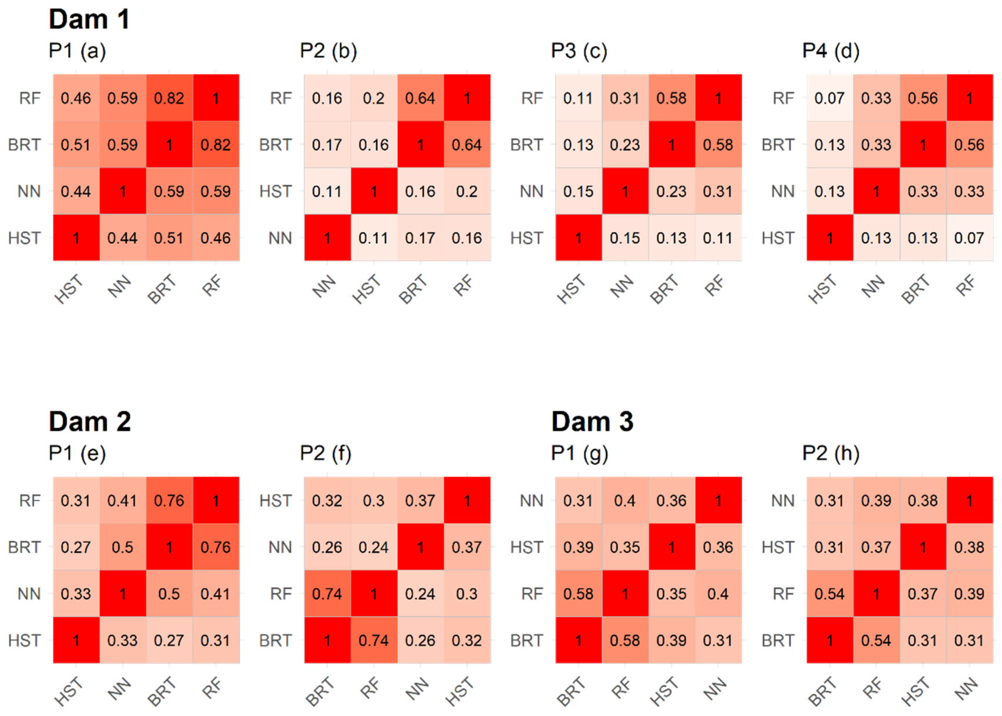
The weight assigned to each expert correlates closely with their accuracy, with greater weight typically allocated to experts exhibiting lower Root-Mean-Square Error (RMSE). Furthermore, the correlation between expert errors, serving as a measure of algorithmic similarity, influences the chosen combination. This phenomenon is exemplified by the BRT and RF weights, which exhibit high error correlation, with BRT proving the more accurate of the two.

The GWA demonstrates the ability to enhance precision, particularly for data records with higher expert error rates. Notably, significant improvement was observed, particularly in the second device of dam 1, with an improvement percentage of 92.23%, compared to the overall improvement percentage of 16.12%. However, no significant improvement was observed in extreme values of the other variables analysed, such as apparatus series, temperature, and reservoir level.

In conclusion, this research underscores the potential benefits of combining accurate experts of varying natures using the Greedy Weighted Algorithm to enhance the precision and reliability of first-level models. Future studies should explore clustering predictions into groups and applying optimised weights based on each record’s group affiliation.