Abstract
In 2030, the world population will exceed 8.5 billion, increasing the challenges to satisfy basic needs for food, shelter, water, and/or energy. Irrigation plays a vital role in productive and sustainable agriculture. In the current context, it is determined not only by water availability but also by optimal management. Several authors have attempted to measure the performance of irrigation networks through various approaches in terms of technical indicators. To improve the sustainability in the pipe sizing of the pressurised irrigation networks, 25 different models were evaluated to discuss the advantages and disadvantages to consider in future methodologies to size water systems, which guarantee the network operation but contribute to improving the sustainability. They enable water managers to use them as tools to reduce a complex evaluation of the performance of a system, and focusing on better management of resources and sustainability indicators for agricultural ecosystems are clear and objective values.
1. Introduction
By 2030, the world’s population will be above 8500 million. Over 800 million inhabitants will add to the current quantity in less than ten years [1]. These substantial increases present several challenges for cover inputs, such as food, shelter, water, and energy. To satisfy them, the United Nations Organisation (UN) estimated necessary increases of 35% in the food supply, 40% in water resources, and 50% in energy to prevent the consequences of several human crises [2,3]. Undeniably, access to available resources is crucial in a rising demand scenario to accomplish the required tasks.
According to experts, in terms of quantity, roughly 3% of the total water on the planet is available for human activities [4]. Among these, the agricultural sector remains the largest consumer of freshwater (Figure 1). Its consumption is around 70% of withdrawals and 90% of consumptive usages, compared to 10% required for municipal purposes or 20% for industrial processes [2,5,6]. For example, rice produced requires around 3400 L of water per kilo. Considering daily water requirements per person are about 100 L, this consumption is equivalent to the domestic needs of 34 people [7,8].
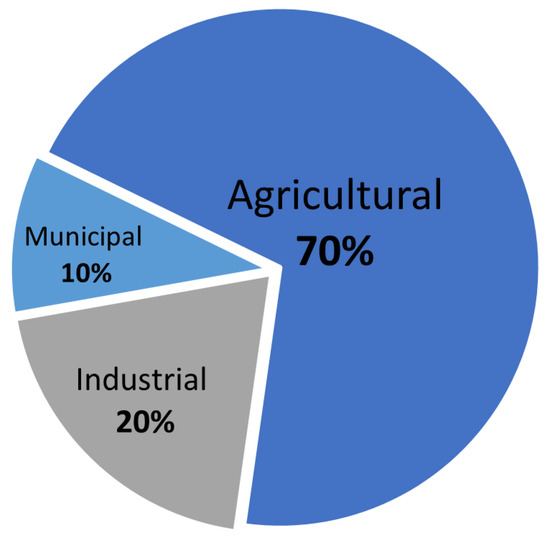
Figure 1.
World freshwater allocation sectors.
Water and energy are inextricably linked; for instance, the water sector is a heavy energy consumer in all life cycle phases: withdrawal, purification, storage, distribution, and treatment. At the same time, the energy generation sector uses extensive amounts of water for all its stages and processes [9,10]. In Europe, an estimated 18% of the total water consumed in energy production is used for cooling [11,12,13]. With a growing population, urbanisation, and rising living standards in many countries, the future picture implicates increased energy use and water consumption [13]. However, several factors can affect the predictions, including efficient and renewable technologies and water-smart energy choices, to achieve a more sustainable integrated water cycle [14,15,16].
Direct and indirect energy inputs are also crucial for the whole chain in agriculture. Supply agri-food production accounts for 30% of the world’s total energy consumption. Irrigated pumping has revolutionised food production, providing 40% of worldwide cereal demand [17]. Nevertheless, despite intensification providing higher efficiency rates, it is directly connected with more energy demands and elevated GHG emissions, putting human mitigation and adaptation aspiration at risk [18,19]. Improving a “climate-smart agriculture” behind and beyond the “farm gate” can achieve substantial savings in water–energy areas, reducing the impact of the food supply system on the environment [18,20,21].
As the environment establishes the initial conditions, societies expand and climate changes; therefore, the vision on energy and water concerns must shift, too. The Paris Agreement and the 2030 Agenda recognise that humanity’s long-term development depends on the sustainable management of resources [22,23]. According to the data, considering a 75% population benefit, the irrigation sector is critical in a sustainable goal contributing to the world’s GDP and global food security [24].
Irrigation plays a vital role in productive and sustainable agriculture [25]. Currently, it is determined not only by water availability since optimal management from project idea to building is necessary for the entire system life cycle [26]. Increasing knowledge about irrigation systems and underlying internal processes improved our understanding of how new conditions affect the systems and how the systems affect the environment. It can provide detailed information and a solid base for a decision maker to develop smart strategies towards a goal.
1.1. Irrigation Water Use
Agriculture is the way to provide the additional billion tons of food needed for consumption shortly. Irrigation is vital for food security in most crops globally, especially in arid and semiarid areas. Furthermore, artificial rainfall makes it possible to provide the required water, nutrition, and pest control with crop growth [27,28,29], as well as diminish drought losses, frost hazards, and climate variability [30].
Moreover, irrigation is a crucial component of rural economies, especially in areas that maintain sustainable local small-scale production and the Mediterranean region [31,32]. Figure 2 shows the world’s irrigated area divided into three groups: developed, developing, and least developing countries, in which the developing countries have a significant role in food production [33]. Nevertheless, poor management represents a high extraction of freshwater resources and energy investment. Likewise, it carries a process of progressive deterioration of the environment. Pollution of wastewater, groundwater table reduction, eutrophication, soil salinisation, displacement of native diversity, significant greenhouse gas emissions (GHGs), and micro-residual pollutants, among other consequences, can lead to unsustainability [34,35].
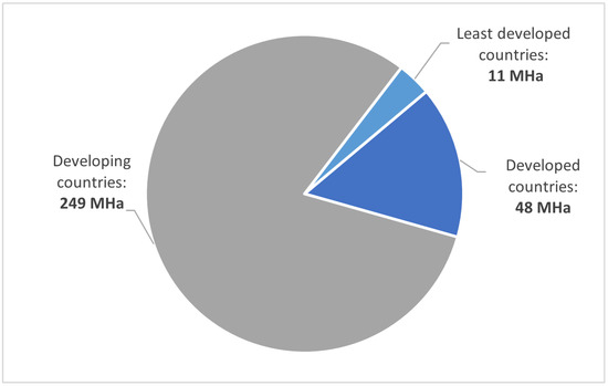
Figure 2.
World irrigated area data from 2021 using data from [33].
Figure 3 shows the different uses (i.e., agricultural, industrial, and urban) in the different continents. It shows that agricultural use represents between 20 and 70% of the consumption. Water use and pollution of resources for growing agriculture will reinforce global water competition for municipal and industrial sectors.
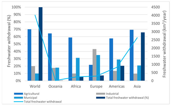
Figure 3.
World water withdrawal. Data obtained from [36].
It is essential to pay attention to discrepancies between low rainfall regions where the water resources are already in sustainable borders, such as Spain’s Mediterranean regions and emerging or developing countries with significant water potential [36,37,38].
Figure 4 shows the high pressure in Mediterranean Europe in the freshwater, especially in Spain.
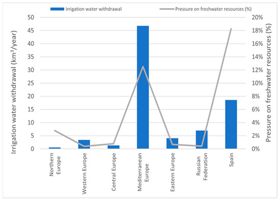
Figure 4.
Water withdrawal. Data obtained from Europe [37] and the world [36,39].
In the unclear future, the key to success relies on the availability of the resources to satisfy user’s needs—enough demand, disposable energy, and acceptable cost for pumping water—without neglecting the environmental premise, which currently must be at the forefront of all the actors involved, especially water decision makers [40].
1.2. Environmental Implications
As an undeniable reality, climate change accelerated due to the current development model built upon fossil energy consumption [41]. High climate variability (temperatures and precipitation patterns), prolonged episodes of drought, and extreme events are recurrent. Those scenarios increase the insecurity in the future management of crop areas, making it necessary to develop models and tools that allow farm viability within a sustainable use of resources [38].
Considering the high stress on non-renewable resources and crop, classical economic criteria must not be the only performance evaluation parameters [42]. Measuring productivity only as a rate between income benefits and inverted monetary inputs in a food production process keeps the misunderstanding of an integral process where multiple costs and benefits interact with economic, environmental, social, and cultural variables in the short, medium, and long term [43].
Given the impossible dissociation between human beings and their surroundings, the stakeholders should introduce performance monitoring instruments to manage complexity in our new paradigm [44]. Identifying components of food supply challenges within agriculture ecosystems, their relationships and boundaries, and the socioeconomic, environmental, and cultural context lets water managers understand the production process because of multiple interconnected factors [45].
As a tool for reducing a complex assessment of a system’s performance, focused on better management of resources, sustainability indicators for agricultural ecosystems are a clear and objective value [46]. Moreover, they also include the correlation between water–energy factors (WF-EFs), the environment (climatic factors (CFs), soil factors (SFs)), socio-cultural factors (SCFs), trade factors (TFs), and gender factors (GFs), among others [18,47,48].
An accurate indicator diagnosis can effectively align exigencies and vulnerabilities, identifying patterns, tendencies, and cause–effect relations in irrigation activities [49]. Indicator benchmarks improve the efficient use of resources, the effectiveness of activities and decisions, equity and the environmental, and the reduction in social impacts. The goal is to ensure long-term resilience systems and sustainable user welfare [50,51,52,53].
The global dimension of water–energy management leads to evaluating the environmental footprint in food production and the entire set of negative and positive responses that agriculture systems impose [54]. Special attention to irrigation systems is justified because these are required in more places. However, its non-negligent critical water needs, inherent pollution, and our uncertain context impose clear boundaries [55].
Considering limitations in environmental and sustainable terms, holistic knowledge of irrigation systems brings a framework to reflect the wide margins of water and energy savings in irrigated agriculture. For instance, in Spain, savings have increased by more than 70% in 15 years [56,57]. Quantifying the performance and constraints of irrigation systems provides a global view of a present system condition and the possible further achievements according to the targets and criteria for appraising the improvements within the water–energy–human nexus. It implies the evaluation of the different sustainability indicators based on different targets of the Sustainable Development Goals [58].
Several authors attempted to measure the performance of irrigation networks by several approaches, such as benchmarking analysis [59], flow-driven deliveries and pressure studies [60,61,62], conventional energy and cost reduction [56], water and energy correlations [63], loss quantification [64], and, finally, water footprint, water use performance, and water savings in environmental and economic viability criteria utilising the effective sustainability irrigation indicators [65,66,67,68,69,70,71].
The present investigation is an evaluation of the different existing methods for estimating peak flow rates to address the design of installations. This stage is crucial not only in the investment of infrastructures but it also impacts the estimation of the evaluation of the different targets of the Sustainable Development Goals (SDGs). Also, approaching the estimation of flow rates with different methodologies can lead to differences in the assessment of sustainability indicators and energy audits that address the installation of micro-hydro generation.
2. Evaluation Methodology and Materials
The research methodology is established in different steps, according to Figure 5.
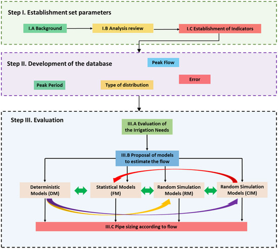
Figure 5.
Evaluation methodology of the models to estimate the circulate flow.
Step I.—Establishment of the parameters. This set is divided into three parts, and a background review is developed to search for the maximum number of proposal models, enabling peak flow estimation. The second step of this block, called I.B analysis review, elaborates a parameter list in which the main variables and characteristics are discretised in the database by indicators or variables (Step I.C).
Step II.—Database development. A database was established using information and data gathered from the consulted bibliographic sources. The indicators utilised in the other examined case studies were chosen to populate the database, encompassing not only measurements and variables but also reference values. It is noteworthy that certain indicators were employed across multiple case studies discussed in the published research. The main variables were peak flow, error between estimation and experimental data, peak period, and type of distribution, among others.
Step III.—This third block constitutes the main block of the research. In the first part (Step III.A), an estimation of the evapotranspiration and possible inputs allowing the development of the different models to determine the peak flow, addressed in Step III.B, was carried out. In this block, a detailed analysis of four different typologies was carried out. A discussion was established evaluating different deterministic, statistical, random, and artificial intelligence models.
According to the review of the background, 45 references were analysed, obtaining 25 different models distributed in Europe, according to Figure 6.
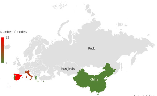
Figure 6.
Distribution of the different analysed models.
3. Determination of Flows to Design Irrigation Water Networks
Whereas measuring water consumed in the municipal sector is usual in most countries and almost essential in the industrial sector, water control in agriculture is not a strict requirement [72]. Nevertheless, assessing water needs is a fundamental part of sustainable water resource use to avoid losses and obtain “more crop per drop” [73,74]. In addition, operating losses throughout the life cycle of the network are difficult to identify and quantify [64].
The lack of control, absence, or inaccuracy causes inefficient use of irrigation, affects expected crops, and generates unnecessary environmental expenses. Boosting food production in uncertain conditions calls for effective and sustainable irrigation management and flexible supplies, which means full appraisal of water–energy deliveries. Qualifying the systems and approaching the knowledge about demands initially imposed on the design process can allow for implementation strategies and plans to improve the profit margin of water–energy inversion [75,76].
Flow and pressure in the network are highly variable throughout the day and the operation cycle. Said variations are closely connected to established area limitations of irrigation systems and decision management in the phenological cycle determined by agroclimatic variables and farmers’ perceptions. The real flows may differ from prior requirements assumed at the design stage, causing operation problems impacting network capacity, demand forecast, and environmental resilience [77].
3.1. Parameters of Study
A realistic approach to the dynamic interactions between water irrigation and sustainability requires modelling the conditions and relations in a farm [78]. These are relative to the cropping patterns demands over the growing process, hydrant discharges, established network design, environmental conditions and reactions, irrigation technology available, and crop responses, as well as user habits along different temporary and spatial scales [79].
To understand these complex interactions in agricultural, biological, and environmental systems and enhance our ability to make predictions, decision makers should study the interconnected components rather than isolating them [80]. A machine learning approach was developed to represent diverse Earth systems models through mathematical relations and schematic concepts nourished with extracted interpretable information from uncountable data sources [81].
Systems models play a primary role in the development of sustainable agroecosystems. Several crop models with different scales of complexity and limitations are available to understand the interaction between soil–water–plant–atmosphere [82]. Different tools have been developed to estimate yield production and the effects of crops that interact with weather resources and management practices [83]. Scientific and decision/policy makers have underpinned the different approaches for increasing the understanding of growing crop processes and the interaction of soil–water–nitrogen along the life cycle, as well as the impacts of cropping patterns and irrigation distribution under climate variability [77,84,85,86].
Different issues emerged in agricultural model sciences developed for researchers and decision maker stakeholders, reinforced by the available data, technology and supporting tools, cost–benefit relation, expected results, and specific targets. Purposeful development of the model, increasing scientific tools, and decision/policy support lead to understanding the agroecological systems improve under research questions about processes control and agroclimatic interactions [85]. Description process, understanding relations, and forecast tools motivate the development of models, which target simplifying complex processes where more of the hypothesis and assumptions are not linked with real cases but decrease uncertainty for reasonable results compared with data from the field.
There are models, which consider the soil–water process, reflected in crop water space–time requirements and water balance [87]. They include calculating the inputs and outputs of the system, effective rainfall, evapotranspiration, and crop requirements using soil, climate, and crop data [88]. Soil moisture varies dynamically and at any time in a crop cycle. Therefore, it is crucial to never drop below the wilting point without exceeding the field capacity [89].
The Penman–Monteith and Priestley–Taylor equations for soil–water relation modelling are highly simplified but widely applicable. According to FAO’s functional model, the physically based approach, FAO-56, allows for the soil–water balance to be obtained following Equation (1) [90].
where rainfall (), irrigation (), and capillary rise () are the inputs of the system. Surface runoff (), water loss out of the root due to deep percolation (), and crop evapotranspiration () are the outputs that compute the soil moisture change ().
Evapotranspiration () is the most important variable in the balance [91]. These phenomenological processes correlate soil evaporation and plant transpiration, which depend on the climate factors, crop characteristics, and water availability in the soil.
In 1998, the FAO-56 ET model was launched. Several definitions and simulation procedures are broadly used following the advances in computing calculation, modern techniques, and tools [92,93].
Climate factors are introduced in this methodology by estimating the daily potential evapotranspiration of a hypothetical parameterised surface—reference evapotranspiration —using Penman–Monteith, described in Equation (2) [90,94].
where detailed energy and aerodynamic data are required, and shortwave radiation at crop surface (), soil heat flux (), air temperature (), wind speed (, psychrometric constant (), relative humidity by saturation vapour pressure deficit (), the slope vapour pressure curve () are found in the equation. Although it is currently used and widely implemented for decades, the accuracy of this method depends on the available data.
Other approaches imply evaluating the reference evapotranspiration when lacking in measures required. The Hargreaves method is proposed as an alternative for assessing with fewer data, only air temperature, as shown in Equation (3) [95,96].
The advantage of this method is that the average daily temperature () and temperature range () are the only values that require a dataset of measures (maximum and minimum daily temperatures). Extraterrestrial radiation () is a tabulated value. This method is recommended for use, especially in the absence of existing data or dubious quality [97].
Secondly, for assessing crop evapotranspiration, the FAO-56 method integrates the crop characteristics (crop type and growth phases) via . This is the dual coefficient that combines soil transpiration and crop evaporation along the development stages [90]. This coefficient is mainly connected to the canopy dynamics, leaf area, and ground cover [98]. Although can be evaluated, crop coefficient tables and curves reported in the literature adjusted to local conditions and midseason periods are widely used [99,100,101].
Thus, it is possible to calculate potential evapotranspiration for a given crop at any moment of its growth following Equation (4).
Another parameter in irrigation that needs quantification is effective rainfall (Pe), a fraction of total valuable rainfall for meeting the water needs to be used by crops, excluding surface runoff, deep percolation, and soil surface evaporation from Equation (1) [102]. FAO-25 describes several approaches for calculating it by the fixed percentage method, the potential evapotranspiration/precipitation ratio method, Renfro equation, empirical relationships, the US Bureau of Reclamation method, and the USDA SCS method [103].
The simplest methodology generally applies a percentage between 70 and 90% of the monthly rainfall. The FAO manual proposes maximum slops in the 4–5% range for Equation (5).
where rainfall or precipitation, in mm, is represented as (, and effective rainfall, mm/month, is .
Equation (6) is used to determine the irrigation net water needs. It shows how these descriptive, empirical, and functional models allow researchers to better understand the relationships between agro-environmental pieces combining physical and biological components and mechanisms, permitting an approach to the possible system’s responses due to certain strategies and decisions adopted within simplified scenarios.
In another approach, dynamic systems can integrate conceptual physical models and mathematical equations with the data collected and provide outputs related to time changes and responses to different externalities, such as climate change or users’ practices [104,105]. Sometimes highly complex, although robust, these models need experts to achieve interpretable results and adapt them to specific issues. However, it is not always a straightforward task due to knowledge gaps, and unavailable data add uncertainty to the outputs [70,106]. Examples of such crop models related to irrigation crop water supply, among others, are FAO agronomic models CROPWAT [107], AquaCrop [69], DSSAT [108], CropSyst [109], and software tools [93].
There is extensive experience developing agroecosystem models, science, and analytics tools [110]. The gaps are primarily related to accurately integrating analytical knowledge into the user’s decision tools [111]. Moreover, various factors are needed to build an integrative agricultural approach, such as the interactions between crops, farms, socioeconomic, cultural, and landscape context, climatic, environmental, and ecological variables, trades, and agro-economic business on different scales [112].
Food security crises, sustainability concerns, technology and computer advances, open information and data accessibility, interdisciplinary and transboundary science, and user-adapted models summarise a new context that must lead to a new generation model focused on management for sustainability and productivity [113].
Agro-crop modelling under an irrigation environment forecasts the amount of water needed, which determines irrigation scheduling, such as when and how much water quantity is necessary to irrigate [114]. Therefore, it is necessary to have integral knowledge of the internal crop process and system input/output estimable responses to decrease uncertainties. Achieving an accurate system’s behaviour characterisation allows the implementation of measures to reduce the water–energy quota invested without the possible detriment of production results expected by farmers.
However, despite the substantial advances in system modelling, the disparity between calculated and real flow demanded is frequently observed. This discrepancy is most often attributable to unpredictable weather conditions, users’ practices, and local management in the present new context of uncertainties [77,115].
3.2. Proposed Methods: Forecasting Irrigation Demand Flow
To determine the flow rate in a distribution system, the complexity of the agricultural ecosystems mentioned must be taken into account [116]. Additionally, particular consideration of the relationships between crop pattern, crop growth stage, water and energy requirements, weather conditions, and users’ interactions must be given. They are several approaches considered for studying the distribution of water discharges and irrigation scheduling for on-demand irrigation networks [117].
Space–time analysis of the randomness process in irrigation was introduced for the flexibility of use and very low probability for a simultaneous operation of all hydrants in a network, which allowed a mathematical approach for calculating the flow distribution. Of all the methods developed, Clément’s first formula (CFF) has had great acceptance since its publication [118].
This formula introduces a statistical analysis for the calculation, implementing a distribution law of probabilities for hydrants’ operation in the network. Given the simple application of the algorithm, this methodology has transcended until today. Despite several errors in simulated flow distribution (since the assumed simplifications are not entirely assured), it is the most widely used method [62,119,120,121]. Nevertheless, the accuracy of these calculations has significant implications for the overall sustainability of the system assessment, such as economic, energetic, hydric budget, flexibility, and safety parameters in all stages, from construction to operation management.
Different approaches have been implemented recently due to technological and computational developments that improve forecasting results. Generally called black box methods, these computational methodologies allow correlating physical parameters with advanced statistical routines to integrate existing uncertainties when correlating inputs and outputs.
Table 1, Table 2, Table 3 and Table 4 summarise some of the most significant research work. According to the methodological approach to influence data and involved variables in the circulating flows forecast, with predictive and management purposes, the methods are differentiated into four groups: deterministic models (D), statistical models (F), random simulation models (R) and computational intelligence models (CI).
3.2.1. Deterministic Models (D)
The deterministic conceptual models—empirical, functional, or mechanistic—assume that uncertainties are external to the process [122]. These models aim to establish a relationship between variables and constants that are well known or measurable and aim to produce “accurate” results under specific facts and considerations. Their theoretical approach does not include random methods [123]. This model entirely determines flow rates by inputs and initial and boundary conditions, and since the model does not contain any haphazard approach to the phenomena, it is necessary to understand and define the problem through a vast set of existing information. Moreover, the methodologies described must gather as much information as possible and use complex models to determine those that cannot be measured directly or introduce any uncertainty.
Ref. [124] simulated the flow distribution in the network using the SIMODIS methodology, where remote sensing satellite data worked under techniques of temporal space evaluation of soil–water balance by the numerical soil–water flow model (SWARP). The studied network was in Gromola (southern Italy) using a daily forecast horizon, a one-year temporal dataset and a 33-day peak period. The model assumes that the network’s hydrograph is a product of implicit needs and boundaries related to biophysical parameters concerning crop water requirements—vegetation status, crop pattern and stage, potential evapotranspiration rates, surface reflectance, soil properties, groundwater interactions, and hydraulic capacity of the network, among others. Comparing the total irrigation daily values from the irrigation season to the simulated data, the method underestimated the volumes by 9%.
Refs. [125,126] conducted two studies, in 2006 and 2008, in a network in Sicily (Italy) with different goals. In the first, the main goal was to create geohydrological models for improving water management in irrigation. Instead, the latter tried to create a distributed model for the assessment of water in irrigation networks. The irrigation phase is scheduled based on two parameters: soil–water pressure head threshold and soil–water deficit to be refilled. Several exposed case studies were conducted, and the outcomes for a simulated Sicilian district were compiled, resulting in overestimating the modelled flows.
Ref. [120] developed a model centred on water balance, simulating the whole irrigation season by calculating the circulating flows through the network at any time based on the soil moisture deficit. This network was in Santaella, Córdoba (southern Spain), with a daily forecast horizon and two years’ worth of data accompanied by a 2-week peak period. Using several climatic and study area characteristics (crop, network, system type, farmer practices) as inputs, the model performs a complete simulation of the irrigation season and provides an hourly consumption on each farm and the operation probability for each event. After evaluating the simulated data and the seasonal volume by year, this method overestimated the demand by 11.6%. The evaluation for each study is summarised in Table 1.

Table 1.
Summarised deterministic models articles reviewed.
Table 1.
Summarised deterministic models articles reviewed.
| ID | Reference | Main Results |
|---|---|---|
| D.1 | [124] |
|
| D.2 | [126] |
|
| D.3 | [120] |
Human behaviour affects uniform probability prediction. |
| D.4 | [125] |
|
3.2.2. Statistical Models (F)
More extended statistical models aim to find a relative frequency associated with different flows during the irrigation season [127]. Through the assumption of certain hypotheses and, despite the random behaviours of some variables, it is possible to arrive at a particular degree of accuracy by utilising an adequate problem definition [128].
These models focus on finding hydrants’ operation probability at a given period, often during peak periods, in the function of maximum crop requirements and own parameters of the probability distribution that describe the system’s behaviour to meet a determined water demand for a given supply [129].
Granados [130] made a detailed description of principal statistical methodologies: Clément, [118,131], de Boissezon and Haït, [132], and Mavropoulos, [133]. Also, he summarised various research works where authors contrast mathematical flows and calibrate parameter implications with real or simulated flows in real irrigation networks.
Clément proposed that flows circulating into the network follow the normal distribution when the number of outlets is significant enough by associating farmers’ activities with hydrant usage as a binomial variable in a Bernoulli experiment, assuming uniform open probability and uniform nominal flow rate downstream of a line section [118,131].
According to Clément’s first formula (CFF), it is possible to determine the downstream flow for a study section using a standardised outlet flow under a service guarantee, as shown in Equation (7).
where the variables are flow to forecast , fixed flow assignment of an outlet , probability operation hydrant and guaranteed service level . The subscript indicates the group of outlets with the same flow assignment and probability.
Mavropoulos [133] changed the perspective and described the system’s performance by defining the oversaturation of the network based on the rate of recurrence of demands in the network, for instance, how unusual or recurrent demand requests are.
The time between two successive irrigation calls, defined as a random variable (r.v.), follows an exponential distribution and is associated with the flow discharged at any time during a peak period using a Weibull distribution. This distribution was selected due to its high flexibility, making it possible to adapt in several flow distribution cases. Equation (8) shows the generalised formula proposed by Mavropoulos and Lotidi [134].
The equation considers variables such as the number of outlets with the same assigned flow , open hydrant probability , shape parameter of the Weibull distribution related to available time use of the network , outlet flow assignment , the time between two demands , and = index that groups uniform population outlets.
Between the articles that pursue the analysis, validation, and contrast of these equations, the results that evaluate the theoretical hypothesis assumed for the models are crucial for future developments.
An entirely random variable is not a precise definition for an open hydrant demand because external factors can influence it. Pulido-Calvo et al. [119] analysed energy tariff constraints that affect farmers’ decisions in the township of Cordoba located in Southwest Spain, using data from 8 years. Their work shows that the probability of outlet operation cannot be the same over the day and defines different probabilities according to different energy cost rates.
Monserrat et al. [121] analysed the CFF model’s hypothesis in networks located in the Ebro River basin (northeast Spain), concluding that only the independent operation of the outlets is satisfied. Setting the daytime irrigation as a preference rejects the random probability. As a result, the calculated flow was underestimated compared to the observed data; a higher standard deviation than calculated in real data, especially connected with human irrigation preferences, is observed.
Ref. [120] also concluded that human behaviour affects predicted probability and shows a more significant deviation in distribution flows due to a greater probability of higher flows. The normal distribution is only shown in a peak period, not according to CFF. Furthermore, after simulating a complete irrigation season in a case study, the gamma distribution was proposed as a better fit with elevated suppleness.
The same appreciation was established by [135] in the network and peak period analysed, where a larger hydrant group operated during weekends in contrast with low cumulative operation on weekdays. This behaviour is justified due to a higher time availability for the farmers and lower energy costs; also, a variable hourly probability operation avoided costly and high evaporation periods.
For Mavropoulos’ method validation, the author published the verification through a real network with registered data for monthly peak irrigation. Despite the good fit found with Weibull’s asymmetric distribution, the uniform probability assumed in the model could not be corroborated. Therefore, introducing λ3, a correction factor, is necessary, representing the non-random farmer’s behaviour and other uncertainties [134].
Unsuccessful demand forecasting and the assumed hypothesis for CFF are also disclosed in the work of Soler et al. [136]. The authors also mention that the flow rate cannot be assumed as a random variable if the number of outlets is not large enough or the operating conditions are not homogeneous.
Ref. [137] conducted various tests to compare CFF’s calculated distribution with observed flow data compiled from a real system. The results showed that the expected normal distribution did not match the observed data in any month of the analysis period. The records had a strong right skew, showing that other distribution functions, such as GEV, could be a better fit. Farmers’ behaviour and preferences like duration, quantity, and hourly and weekly trends can explain the gap between data. As exposed by Pérez-Sánchez et al. [138], human influence determines irrigation patterns, and it is unreasonable to consider uniform probability as a valid hypothesis for forecasting irrigation flows.
Table 2.
Summarised statistical models articles reviewed.
Table 2.
Summarised statistical models articles reviewed.
| ID | Reference | Type | Main Results |
|---|---|---|---|
| S.1 | [119] | Statistical |
|
| S.2 | [121] | Frequentist |
Moreover, the model with Clément’s first formula seems robust enough in the conditions studied, so using more complicated models is unnecessary |
| S.3 | [120] | Deterministic |
|
| S.4 | [134] | Statistical |
|
| S.5 | [135] | Random Simulation |
The underestimation caused by the Clément methodology is due to using the average opening hydrant probability concept. |
| S.6 | [137] | Statistical |
|
3.2.3. Random Simulation Models (R)
Random simulation models focus on system behaviour analysis through a random approach. The target is a model configuring the relations between variables associated with the portion of the irrigation problem that cannot be known accurately, thus introducing uncertainty to the results.
Some parameters influenced by uncertainties are defined randomly within established assumptions and scopes. Often used for performance analyses of existing networks, these models propose considering stochastic flow variability due to farmers’ management strategies. Defined by the users’ decisions related to the perception of crop stage, the number and location of open hydrants define the complete system performance [139]. Also, the flow rate is a product of a random computer simulation, a random variable within a sample space of possible events, which can include potential combinations satisfying the corresponding constraints and integral network spatial–time variability.
After considering the CFF model, Soler et al. [136] proposed calculating the flow rate distribution as a non-normalised random variable; they implemented two random methods based on the number of downstream outlets of the section analysed. Thus, the first step was to create a complete sample space of irrigation events. Associates knew the constant operation probability for each hydrant, the corresponding nominative discharge with a randomly generated vector, and the operational state of the hydrant (on/off) configured by 1 or 0, respectively.
When the number of hydrants is sufficient, the authors used the Monte Carlo approach to build an incomplete sample space according to known probability and discharge rates.
where the jth-event on/off vector is , the total number of event vectors is the probability for the event is the nominal flow rate is , and the index for each hydrant is .
where is the discrete random variable flow vector, is the probability density function, and is the cumulative distribution function.
On the other hand, Labye [140] introduced it as part of the design process considering the temporal variability of flows circulating through the network and the importance of Several Flow Regimes (SFR approach). Likewise, as opposed to the “only a single flow”, Lamaddalena et al. [141] provide a Random Generated Model (RGM) for obtaining different combinations of hydrants simultaneously open among the total of hydrants in the network, satisfying a given discharge and considering an upstream demand hydrograph at the end of the network as an input.
The flow circulating in a specific section is calculated by adding the discharges withdrawn from the downstream open hydrants. This tool serves different purposes, such as analysing an existing network or designing a new one while computing the upstream end demand input by a CFF-based model.
In a different approach, without considering an average operation probability, Moreno et al. [135] assumed a random starting opening time for the hydrants and the irrigation set time for each one according to the cropping requirements and the crop yield characteristics. The method builds vast Random Daily Demand Curves through a dataset of open hydrants and the operation time of the network.
Adding these open hydrants makes it possible to calculate the total demand upstream of the study section in a determined time. Obtaining the main line flow associated with an operational quality service is possible. The case study provides a good fit between measured and calculated data.
Table 3.
Summarised random models.
Table 3.
Summarised random models.
| ID | Reference | Conclusions |
|---|---|---|
| R.1 | [141] |
|
| R.2 | [142] |
|
| R.3 | [143] |
|
| R.4 | [135] |
|
| R.5 | [144] |
|
| R.6 | [136] |
|
| R.7 | [145] |
|
Hybrid models exposed by Khadra et al. [139,141], Calejo et al. [142], Zaccaria et al. [144], and Fouial et al. [145] are a combination of deterministic and random stochastic models. They assume the presence of variables within the model requiring random treatment due to wider spatial–temporary variability, higher uncertainty contribution in the process, and low viability to assess an accurate soil–water balance.
Deterministic components, water budget, and crop requirements are estimated utilising the soil–water balance at the plot irrigated level. Uncertainties and variability of some parameters, such as those introduced by the farmers’ management decisions—seed day, irrigation depths, irrigation efficiencies, and starting irrigation time—are modelled by a stochastic approach.
Similarly, Pérez-Sánchez et al. [138] proposed a new methodology for determining flow allocations, crop water demand, and consumption patterns, which are considered by a deterministic approach. Assuming indeterminate irrigation farmers’ habits are the stochastic part, and the model included weekly and hourly trends and the irrigation duration using information about users’ behaviour obtained from farm interviews.
3.2.4. Computational Intelligence Models (CI)
Fourthly, some proposals face the complex problem of flow distribution in the networks in a varying and uncertain environment under the influence of knowing computational intelligence models. Focused on understanding systems’ behaviour through the design of “intelligent agents” that represent real problems, these models propose applications that exhibit an ability to learn from historical data and adapt it to predict new data, inspired by the biological and organisational models [146,147].
The branches composing the computational intelligence that promotes efficient forecasting solutions include fuzzy logic, decision trees, neural networks, and evolutionary algorithm models [148].
Krupakar et al. [149] performed a comparative analyses of a broad spectrum of methods regarding the performance and accuracy of predictions. Some of the analysed methods are summarised below.
A Computational Neural Network, CNN, is a non-linear mathematical structure that tries to reproduce the human brain’s performance to solve problems and its ability to replicate complex non-linear problems, finding patterns and correlations. Learning from the relations between inputs and outputs allows it to apply the knowledge acquired to solve different situations in a new context [150,151].
The performance of CNN models in predicting water irrigation demands was presented by Pulido Calvo et al. [152], taking past and present data on water demands and climatic and crop parameters as inputs.
In a four-layer feed-forward CNN structure (i.e., in a model where the previous information travels only in one way from the input to output layers and with hidden layers), a learning–training algorithm to determine the interconnecting weights between the nodes and neurons of each layer is implemented.
Activation functions were linear, and sigmoidal non-linear functions were used for the output layer and hidden layers, respectively. The controlled index chosen for the model was the determination coefficient ().
Fuzzy logic rules (FL) introduce the mathematics of fuzzy theory [153], which allows one to study and describe the systems within a scale that includes partial values, such as the Boolean logic of zeros (0) and ones (1), gaining knowledge of the information that involves a certain degree of uncertainty.
This alternative to the binary systems resembles the human decision procedure that can make a choice based on the information with much imprecision, such as “it is warm” or “it is wet”, traducing it in clear values through the assigned relation functions [154]. Genetic algorithms (GAs) are used to find the optimum solution to complex problems. This approach is inspired by natural selection and heritage principles, where through crossovers, selection, and mutation rules, the initial populations defined “evolve” to better individuals as a better solution, improving their characteristics generation after generation.
A defined objective function evaluates the fitness of each new individual generated, and a constraint set penalises those who violate them [155].
Multiple regression models are used to obtain a linear equation that explains the phenomena targeted to predict dependent variables by knowing independent variables and the assigned contributions of each one to these estimations [156].
Pulido-Calvo et al. [157] implemented multiple regression for predicting daily water consumed as a dependent variable in irrigation models. In a best-proposed model, the water demand of the previous two days was recorded on a farm by a telemetry system installed as input knowing variables. Equation (11) shows the linear equation obtained for a calibrated analysis period for olive crop farms.
where is the estimated consumption on day t and and are the observed demands at one and two days before t, respectively.
Large amounts of information and variables can complicate any model and reduce the precision due to high correlations between its components. Wang et al. [158] implemented a regression analysis method to face this problem using Principal Component Analysis (PCA) methods to identify the main factors influencing water demand, keeping as much information as possible while reducing the large amounts of inputs in a multiple-factor irrigation space.
Results show that the contribution of precipitation and irrigated areas have the strongest influence among the analysed factors. Both are used in a linear regression method in addition to a water-saving coefficient representing the human influence on irrigation demand.
This coefficient includes planting structure adjustment and water-saving technologies, which can change the water demand required year by year. Equation (12) represents the function of the water demand for irrigation.
where is the predicted amount of water, is the precipitation, is the irrigation area, is the annual average water saving coefficient, is the forecasting year, and is the data series corresponding to the first year.
To capitalise on the strength of several models and enhance their entire performance, combining them to create hybrid models is possible. Ref. [151] developed a model combining different paradigms from CI, such as a feed-forward CNN, fuzzy logic, and genetic algorithms, to forecast daily irrigation district demands, taking only the historical data series as the input. According to the authors, the predictive capacity of this model is explained by its remarkable ability to extract the highly variable and unstable underlying patterns of the time series data.
In further work, Ref. [159] opted for the Evolutionary Robotic method (ER), which obtains the best CNN and integrates the capacity of the GA to improve precision. This method created an optimal ANGN (Artificial Neuro-Genetic Network) for a short-term (daily) forecast of irrigation demands at the district level. A GA was used to achieve the optimal parameters that structure the CNN to forecast with maximal accuracy and minimal error estimation.
After correlation analysis, the model reduced the data to twenty-seven possible weather inputs and daily historical water register data and selected seven of the best inputs to achieve the singular water demand output.
Although the model has excellent performance, matching observed and simulated data with small datasets and simulation time shows that for the peak demands, the lack of accuracy is present for the three best CNNs. The article refers to various reasons, such as a lack of adequately trained patterns with extreme values.
In another hybrid method, Ref. [160] predicted the amount of water applied on a farm. Likewise, this work combines the three methodologies (CNN, FL, and GA). Fuzzy logic was used to select relevant inputs from the vast irrigation space information and to model farmers’ behaviour related to local practices, empirical thermal sensation, or holiday appreciation. Genetic algorithms were implemented to optimally split the linguistic universe for each variable (e.g., “it is warm”) to be transformed in a range of mathematical inference sets.
Input variables that directly correlate with applied water forecast were, for this work, irrigation depth water from the previous and two previous days; the thermal sensation can also condition farmers’ irrigation decisions. Trained with three different crops in an irrigation district, the analysis model shows that cultural and local practices defined for users’ demands can differ for each crop, even when the irrigation system stays the same.
Accenting the relations between dataset attributes inputs and expected forecast outputs, decision tree models (DT) are structures with internal and external nodes, decision functions, and terminal data results, connected by branches that search for understanding logic rules between them.
Ref. [161] used the DT model to focus attention on when the irrigation event occurs at the farm level. As a binary occurrence problem capable of better-replicating farmers’ behaviour, a DT was built starting with an irrigation process input vector, which included weather, phenological plant state, local practices, and daily hydrant operation, and was explicitly selected for a case study and split into two main classes.
A multi-objective GA selected the optimal tree structure. The accuracy of predicted event occurrences for the best DT designed was very high, between 90 and 100% of irrigation events in a real network.
Table 4.
Summarised computer intelligence models articles reviewed.
Table 4.
Summarised computer intelligence models articles reviewed.
| ID | Reference | Model Type | Conclusions |
|---|---|---|---|
| CI.1 | [152] | Computational Neural Networks (CNNs) |
|
| CI.2 | [157] | Linear Regressions and Computational Neural Networks (CNNs) |
|
| CI.3 | [151] | Hybrid Computational Neural Networks + Fuzzy Logic + Genetic Algorithm (CNNs + FL + GA) |
|
| CI.4 | [159] | Artificial Neuro-Genetic Networks (ANGNs) |
|
| CI.5 | [158] | Principal Component Analysis (PCA) + Regression Analysis Methods |
|
| CI.6 | [160] | Hybrid Computational Neural Networks + Fuzzy Logic + Genetic Algorithm (CNNs + FL + GA) |
|
| CI.7 | [161] | Decision Trees + Genetic Algorithm (DTs + GA) |
|
3.3. Flow Pipe Sizing: Indicators
The use of the different methodologies, as well as the study of opening probabilities as a function of the flow assessment and the estimation model, allows water managers to obtain different flow distributions over time. These distributions, which are different according to the chosen method (different colours), are represented schematically in Figure 7. Defining the design value and the best estimate is crucial in the design and subsequent management of water infrastructure.
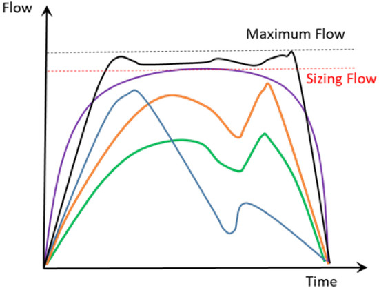
Figure 7.
Distribution of flow over time.
As shown in Table 5, which includes 20 different distribution networks, the uniqueness of the network and its topology implies that the values of flow, leakage, and energy consumed (and thus CO2 emitted) are different. Therefore, the analysis of flow distributions is crucial to address the design and subsequent management of distribution systems.
Table 5.
Variation of the flow, leakage, and annual consumed energy in irrigation networks.
Flow distributions not only involve energy consumption and CO2 water footprint, but the construction of the network itself involves CO2 emissions for each metre of pipeline installed when taking into account the creation, excavation, transport, and execution of the irrigation system works, as shown in Figure 8,which shows that the variation of CO2 emitted varies between 50 and 150% as a function of the diameter and the material.
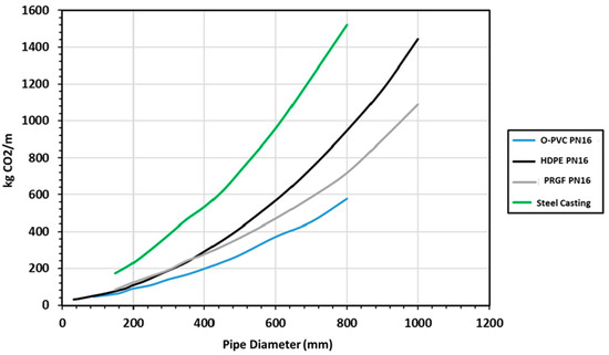
Figure 8.
Distribution of the different analysed models.
4. Conclusions
To accurately forecast irrigation demands, agronomic variables have a key role. Moreover, relationships between crop patterns, crop group stage, water and energy requirements, weather conditions, and user interactions should be considered. Various approaches have been developed, resulting in different methodologies showing the different methods to estimate the maximum flow to size the different pipes of water irritation networks.
This paper shows some of the most important articles supporting different methods for forecasting irrigation demand. Based on the variables involved, the methods are classified into four groups: (i) deterministic models (D), in which it is assumed that uncertainties are external to the process, and they need to gather as much information as possible, and (ii) statistical models (F), which aim to determine the relative frequency corresponding to different flows during the irrigation season. The main goal is obtaining the operation probability of the hydrants at a given period. (iii) Random simulation models (R) consider a random approach of variables by creating and assuming relationships with the components associated with the portion of the irrigation that cannot be known accurately. They be influenced by uncertainties or within established assumptions and scopes. (iv) Computational intelligence models (CI) can learn from historical data and use them to predict new values based on patterns and series inspired by the biological and organisational models. The comparison of the different methods was focused on the adjustment of the function and a better definition of the maximum flow rate that allows the design flow rate to be established. Addressing and/or knowing the best flow frequency distribution function according to statistical function settings can lead to improved irrigation network design and management methods in terms of sustainability and investment.
Computer intelligence science is implemented in many fields and transforming water management concepts. Progress in this area and data collection technology allow modelling variables, such as human behaviour, thus finding relationships between expected water demands and weather conditions, water applied in previous days, and even the users’ thermal sensations.
It is powerful to learn from experience and quickly adapt to new information. Moreover, it is used to create robust models for getting into advanced irrigation management, saving considerable water volumes and energy and leading to better planning for each irrigation season and day-to-day operation time.
A study of the influence of flow distribution in distribution networks, considering its influence on energy consumption, the possible installation of micro-hydraulic generation systems, and its sustainability in terms of infrastructure implementation and operation, is necessary to address sustainable management of irrigated agriculture.
Author Contributions
Conceptualisation, F.-J.S.-R. and M.P.-S.; methodology, M.A.G.-E. and M.P.-S.; formal analysis, M.A.G.-E.; investigation, M.A.G.-E.; writing—original draft preparation, M.A.G.-E. and M.P.-S.; visualisation, P.A.L.-J.; supervision, M.P.-S. All authors have read and agreed to the published version of the manuscript.
Funding
This research was funded by 2017–2020 PID2020-114781RA-I00 and MCIN/AEI/10.13039/501100011033.
Data Availability Statement
Data are contained within the article.
Conflicts of Interest
The authors declare no conflicts of interest.
Abbreviation
List of acronyms and abbreviations used in this article.
| CFF | Clément’s first formula |
| CNNs | Computer Neuronal Networks |
| DESA | Department of Economic and Social Affairs |
| DESA | Department of Economic and Social Affairs |
| FAO | Food and Agriculture of the United Nations |
| EEA | European Environmental Agency |
| ICID | International Commission on Irrigation and Drainage |
| IPCC | International Panel on Climate Change |
| IWMI | International Water Management Institute |
| RGM | Random Generated Model |
| SFRs | Several Flow Regimes |
| UN | United Nations |
| UN | United Nations |
| WEF | World Economic Forum |
| WWAP | United Nations World Water Assessment Programme |
| WWDR | World Water Development Report |
| Shape parameter of the Weibull distribution | |
| Annual average water saving coefficient | |
| Soil moisture change | |
| Slope vapour pressure | |
| Psychrometric constant | |
| Outlet flow assignment of group i | |
| Water loss out of the root due to deep percolation | |
| Fixed flow assignment of outlet group i | |
| Crop evapotranspiration | |
| Reference evapotranspiration | |
| Relative humidity by saturation vapour pressure deficit | |
| Irrigation area | |
| Cumulative distribution function (cdf) | |
| Probability density function | |
| Soil heat flux | |
| Irrigation | |
| Net irrigation water needs | |
| Crop coefficient | |
| Vector representing the jth event | |
| Total number of vectors analysed | |
| Number of outlets with the same assigned flow at group i | |
| Precipitation; rainfall | |
| Effective rainfall | |
| Probability of Q being Qi | |
| Probability of the operation of hydrant group i | |
| Discrete random variable flow vector | |
| Estimated water demand in day t | |
| Flow to forecast (Clément’s first formula) | |
| Observed water demand in day t − 1 | |
| Observed water demand in day t − 2 | |
| Nominal flow rate of vector i | |
| Surface runoff | |
| Extraterrestrial radiation | |
| Radiation at crop surface | |
| Rainfall | |
| Air temperature | |
| Temperature range | |
| Average daily temperature | |
| Forecasting year | |
| Data series corresponding to the first year | |
| Time between two demands in group i | |
| Guaranteed service level of group i | |
| Wind speed | |
| Predicted amount of water demanded | |
| Capillary rise |
References
- United Nations. World Population Prospects 2019—Highlights; Department of Economic and Social Affairs: New York, NY, USA, 2019. [Google Scholar]
- WWDR; UN. Water and Energy, The United Nations World Water Development Report 2014 (2 Volumes). UN World Water Assessment Programme; UNESCO: Paris, France, 2014; Available online: http://unesdoc.unesco.org/images/0022/002257 (accessed on 25 March 2024).
- World Economic Forum. The Global Risks Report 2018 13th Edition; World Economic Forum: Geneva, Switzerland, 2013; Volume 14. [Google Scholar]
- FAO. Water for Sustainable Food and Agriculture a Report Produced for the G20 Presidency of Germany; FAO: Rome, Italy, 2017. [Google Scholar]
- Zhang, D.D.; Lee, H.F.; Wang, C.; Li, B.; Pei, Q.; Zhang, J.; An, Y. The Causality Analysis of Climate Change and Large-Scale Human Crisis. Proc. Natl. Acad. Sci. USA 2011, 108, 17296–17301. [Google Scholar] [CrossRef] [PubMed]
- UNESCO World Water Assessment Program. The United Nations World Water Development Report 2019: Leaving No One Behind; UNESCO: Paris, France, 2019. [Google Scholar]
- Harper, C.; Snowden, M. Environment and Society: Human Perspectives on Environmental Issues; Routledge: New York, NY, USA, 2017; pp. 1–447. [Google Scholar] [CrossRef]
- Chapagain, A.K.; Hoekstra, A.Y. The Blue, Green and Grey Water Footprint of Rice from Production and Consumption Perspectives. Ecol. Econ. 2011, 70, 749–758. [Google Scholar] [CrossRef]
- Flammini, A.; Puri, M.; Pluschke, L.; Dubois, O. Walking the Nexus Talk: Assessing the Water-Energy-Food Nexus in the Context of the Sustainable Energy for All Initiative; FAO: Rome, Italy, 2014; ISBN 9251084874. [Google Scholar]
- Bauer, D.; Philbrick, M.; Vallario, B.; Battey, H.; Clement, Z.; Fields, F. The Water-Energy Nexus: Challenges and Opportunities; US Department of Energy: Washington, DC, USA, 2014. [Google Scholar]
- EEA. The European Environment: State and Outlook 2020: Knowledge for Transition to a Sustainable Europe; European Environment Agency: Copenhagen, Denmark, 2019; ISBN 978-92-9480-090-9. [Google Scholar]
- EEA. Use of Freshwater Resources in Europe—European Environment Agency. Available online: https://www.eea.europa.eu/ims/use-of-freshwater-resources-in-europe-1?utm_source=EEASubscriptions&utm_medium=RSSFeeds&utm_campaign=Generic (accessed on 4 August 2022).
- Del Borghi, A.; Moreschi, L.; Gallo, M. Circular Economy Approach to Reduce Water–Energy–Food Nexus. Curr. Opin. Environ. Sci. Health 2020, 13, 23–28. [Google Scholar] [CrossRef]
- Kohli, A.; Frenken, K. Cooling Water for Energy Generation and Its Impact on National-Level Water Statistics; Food and Agriculture Organization: Rome, Italy, 2011. [Google Scholar]
- Averyt, K.B.; Fisher, J.B.; Huber-Lee, A.T.; Lewis, A.; Macknick, J.; Madden, N.T.; Rogers, J.; Tellinghuisen, S. Freshwater Use by US Power Plants Electricity’s Thirst for a Precious Resource: A Report of the Energy and Water in a Warming World Initiative; NREL/TP-6A20-53273; Union of Concerned Scientists: Cambridge, MA, USA, 2011; 62p. [Google Scholar]
- Kanakoudis, V.; Tsitsifli, S.; Zouboulis, A.I. WATERLOSS Project: Developing from Theory to Practice an Integrated Approach towards NRW Reduction in Urban Water Systems. Desalination Water Treat. 2015, 54, 2147–2157. [Google Scholar] [CrossRef]
- FAO. Energy-Smart Food for People and Climate; FAO: Rome, Italy, 2011. [Google Scholar]
- FAO. Climate-Smart Agriculture Sourcebook; Palombi, L., Sessa, R., Eds.; FAO: Rome, Italy, 2014; ISBN 978-92-5-107720-7. [Google Scholar]
- Daccache, A.; Ciurana, J.S.; Rodriguez Diaz, J.A.; Knox, J.W. Water and Energy Footprint of Irrigated Agriculture in the Mediterranean Region. Environ. Res. Lett. 2014, 9, 124014. [Google Scholar] [CrossRef]
- Tilman, D.; Clark, M. Food, Agriculture & the Environment: Can We Feed the World & Save the Earth? Daedalus 2015, 144, 8–23. [Google Scholar] [CrossRef]
- Godfray, H.C.J.; Beddington, J.R.; Crute, I.R.; Haddad, L.; Lawrence, D.; Muir, J.F.; Pretty, J.; Robinson, S.; Thomas, S.M.; Toulmin, C. Food Security: The Challenge of Feeding 9 Billion People. Science (1979) 2010, 327, 812–818. [Google Scholar] [CrossRef] [PubMed]
- United Nations. Transforming Our World: The 2030 Agenda for Sustainable Development United Nations United Nations Transforming Our World: The 2030 Agenda for Sustainable Development; United Nations: New York, NY, USA, 2015. [Google Scholar]
- United Nations. Adoption of the Paris Agreement. In Proceedings of the Conference of the Parties on Its Twenty-First Session, Paris, France, 30 November–13 December 2015. [Google Scholar]
- Rai, R.K.; Singh, V.P.; Upadhyay, A. Planning and Evaluation of Irrigation Projects: Methods and Implementation; Academic Press: Cambridge, MA, USA, 2017. [Google Scholar]
- Wang, Y.; Zhou, Y.; Franz, K.J.; Zhang, X.; Qi, J.; Jia, G.; Yang, Y. Irrigation Plays Significantly Different Roles in Influencing Hydrological Processes in Two Breadbasket Regions. Sci. Total Environ. 2022, 844, 157253. [Google Scholar] [CrossRef] [PubMed]
- Ben-Alon, L.; Loftness, V.; Harries, K.A.; Cochran Hameen, E. Life Cycle Assessment (LCA) of Natural vs Conventional Building Assemblies. Renew. Sustain. Energy Rev. 2021, 144, 110951. [Google Scholar] [CrossRef]
- Chartzoulakis, K.; Bertaki, M. Sustainable Water Management in Agriculture under Climate Change. Agric. Agric. Sci. Procedia 2015, 4, 88–98. [Google Scholar] [CrossRef]
- FAO. The State of the World’s Land and Water Resources for Food and Agriculture (SOLAW). Available online: https://www.fao.org/nr/solaw/solaw-home/en/ (accessed on 4 August 2022).
- de Vrese, P.; Hagemann, S.; Claussen, M. Asian Irrigation, African Rain: Remote Impacts of Irrigation. Geophys. Res. Lett. 2016, 43, 3737–3745. [Google Scholar] [CrossRef]
- Olayide, O.E.; Tetteh, I.K.; Popoola, L. Differential Impacts of Rainfall and Irrigation on Agricultural Production in Nigeria: Any Lessons for Climate-Smart Agriculture? Agric. Water Manag. 2016, 178, 30–36. [Google Scholar] [CrossRef]
- Rodríguez Díaz, J.A.; Weatherhead, E.K.; Knox, J.W.; Camacho, E. Climate Change Impacts on Irrigation Water Requirements in the Guadalquivir River Basin in Spain. Reg. Environ. Change 2007, 7, 149–159. [Google Scholar] [CrossRef]
- Moragues-Faus, A. How Is Agriculture Reproduced? Unfolding Farmers’ Interdependencies in Small-Scale Mediterranean Olive Oil Production. J. Rural Stud. 2014, 34, 139–151. [Google Scholar] [CrossRef]
- ICID. World Irrigated Area—2021. Available online: https://icid-ciid.org/Knowledge/world_irrigated_area/ (accessed on 4 August 2022).
- García-Tejero, I.F.; Durán-Zuazo, V.H.; Muriel-Fernández, J.L.; Rodríguez-Pleguezuelo, C.R. Water and Sustainable Agriculture; Springer: Dordrecht, The Netherlands, 2011; pp. 1–94. [Google Scholar] [CrossRef]
- Fernández-Cirelli, A.; Arumí, J.L.; Rivera, D.; Boochs, P.W. Environmental Effects of Irrigation in Arid and Semi-Arid Regions. Chil. J. Agric. Res. 2009, 69, 27–40. [Google Scholar] [CrossRef]
- Frenken, K.; Gillet, V. Irrigation Water Requirement and Water Withdrawal by Country; FAO: Rome, Italy, 2012. [Google Scholar]
- Eliasson, Å.; Faurès, J.-M.; Frenken, K.; Hoogeveen, J. AQUASTAT—Getting to Grips with Water Information for Agriculture; FAO: Rome, Italy, 2003; Available online: https://www.fao.org/statistics/methods-and-standards/general/en (accessed on 15 January 2024).
- IPCC. Climate Change and Land; IPCC: Geneva, Switzerland, 2019. [Google Scholar]
- FAO. AQUASTAT—FAO’s Global Information System on Water and Agriculture. Available online: https://www.fao.org/aquastat/en/ (accessed on 4 August 2022).
- Kehrein, P.; Van Loosdrecht, M.; Osseweijer, P.; Garfí, M.; Dewulf, J.; Posada, J. A Critical Review of Resource Recovery from Municipal Wastewater Treatment Plants—Market Supply Potentials, Technologies and Bottlenecks. Environ. Sci. 2020, 6, 877–910. [Google Scholar] [CrossRef]
- Corwin, D.L. Climate Change Impacts on Soil Salinity in Agricultural Areas. Eur. J. Soil Sci. 2021, 72, 842–862. [Google Scholar] [CrossRef]
- Roga, S.; Bardhan, S.; Kumar, Y.; Dubey, S.K. Recent Technology and Challenges of Wind Energy Generation: A Review. Sustain. Energy Technol. Assess. 2022, 52, 102239. [Google Scholar] [CrossRef]
- O’Donnell, C.J. Measuring and Decomposing Agricultural Productivity and Profitability Change. Aust. J. Agric. Resour. Econ. 2010, 54, 527–560. [Google Scholar] [CrossRef]
- Arduini, S.; Manzo, M.; Beck, T. Corporate Reputation and Culture: The Link between Knowledge Management and Sustainability. J. Knowl. Manag. 2023. ahead-of-print. [Google Scholar] [CrossRef]
- Sharma, R.; Kamble, S.S.; Gunasekaran, A.; Kumar, V.; Kumar, A. A Systematic Literature Review on Machine Learning Applications for Sustainable Agriculture Supply Chain Performance. Comput. Oper. Res. 2020, 119, 104926. [Google Scholar] [CrossRef]
- Olabi, A.G.; Obaideen, K.; Elsaid, K.; Wilberforce, T.; Sayed, E.T.; Maghrabie, H.M.; Abdelkareem, M.A. Assessment of the Pre-Combustion Carbon Capture Contribution into Sustainable Development Goals SDGs Using Novel Indicators. Renew. Sustain. Energy Rev. 2022, 153, 111710. [Google Scholar] [CrossRef]
- Alvarez Morales, Y. Evaluación de Indicadores de Sustentabilidad Agroecológica En Sistemas de Producción Agrícola de Baja California Sur, México; CIBNOR: La Paz, Mexico, 2015. [Google Scholar]
- Seager, J. Sex-Disaggregated Indicators for Water Assessment, Monitoring and Reporting; UNESCO Publishing: Paris, France, 2015; ISBN 9231001191. [Google Scholar]
- Islam, M.S.; Rahman, M.N.; Ritu, N.S.; Rahman, M.S.; Sarker, M.N.I. Impact of COVID-19 on Urban Environment in Developing Countries: Case Study and Environmental Sustainability Strategy in Bangladesh. Green Technol. Sustain. 2024, 2, 100074. [Google Scholar] [CrossRef]
- Nogueira Vilanova, M.R.; Filho, P.M.; Perrella Balestieri, J.A. Performance Measurement and Indicators for Water Supply Management: Review and International Cases. Renew. Sustain. Energy Rev. 2015, 43, 1–12. [Google Scholar] [CrossRef]
- UNDP Human Development Index | Human Development Reports. Available online: https://hdr.undp.org/data-center/human-development-index#/indicies/HDI (accessed on 4 August 2022).
- Delang, C.O.; Yu, Y.H. MEASURING WELFARE BEYOND ECONOMICS: The Genuine Progress of Hong Kong and Singapore; Routledge: New York, NY, USA, 2019; ISBN 9780367332853. [Google Scholar]
- Schepelmann, P.; Goossens, Y.; Makipaa, A. Towards Sustainable Development: Alternatives to GDP for Measuring Progress; Wuppertal Spezial: Wuppertal, Germany, 2009; ISBN 3929944812. [Google Scholar]
- Wang, X.C.; Jiang, P.; Yang, L.; Van Fan, Y.; Klemeš, J.J.; Wang, Y. Extended Water-Energy Nexus Contribution to Environmentally-Related Sustainable Development Goals. Renew. Sustain. Energy Rev. 2021, 150, 111485. [Google Scholar] [CrossRef]
- Tucker, K.; Stone, W.; Botes, M.; Feil, E.J.; Wolfaardt, G.M. Wastewater Treatment Works: A Last Line of Defense for Preventing Antibiotic Resistance Entry Into the Environment. Front. Water 2022, 4, 883282. [Google Scholar] [CrossRef]
- Carrillo-Cobo, M.T.; Camacho-Poyato, E.; Montesinos, P.; Rodriguez-Diaz, J.A. Assessing the Potential of Solar Energy in Pressurized Irrigation Networks. The Case of Bembézar MI Irrigation District (Spain). Span. J. Agric. Res. 2014, 12, 838–849. [Google Scholar] [CrossRef]
- Tarjuelo, J.M.; Rodriguez-Diaz, J.A.; Abadía, R.; Camacho, E.; Rocamora, C.; Moreno, M.A. Efficient Water and Energy Use in Irrigation Modernization: Lessons from Spanish Case Studies. Agric. Water Manag. 2015, 162, 67–77. [Google Scholar] [CrossRef]
- Garcia, C.; López-Jiménez, P.A.; Sánchez-Romero, F.J.; Pérez-Sánchez, M. Assessing Water Urban Systems to the Compliance of SDGs through Sustainability Indicators. Implementation in the Valencian Community. Sustain. Cities Soc. 2023, 96, 104704. [Google Scholar] [CrossRef]
- Rodríguez-Díaz, J.A.; Camacho-Poyato, E.; López-Luque, R.; Pérez-Urrestarazu, L. Benchmarking and Multivariate Data Analysis Techniques for Improving the Efficiency of Irrigation Districts: An Application in Spain. Agric. Syst. 2008, 96, 250–259. [Google Scholar] [CrossRef]
- Fernández García, I.; Rodríguez Díaz, J.A.; Camacho Poyato, E.; Montesinos, P. Optimal operation of pressurized irrigation networks with several supply sources. Water Resour. Manag. 2013, 27, 2855–2869. [Google Scholar] [CrossRef]
- Pereira, L.S.; Calejo, M.J.; Lamaddalena, N.; Douieb, A.; Bounoua, R. Design and Performance Analysis of Low Pressure Irrigation Distribution Systems. Irrig. Drain. Syst. 2003, 17, 305–324. [Google Scholar] [CrossRef]
- Calejo, M.J.; Lamaddalena, N.; Teixeira, J.L.; Pereira, L.S. Performance analysis of pressurized irrigation systems operating on-demand using flow-driven simulation models. Agric. Water Manag. 2008, 95, 154–162. [Google Scholar] [CrossRef]
- Rodríguez Díaz, J.A.; Camacho Poyato, E.; Blanco Pérez, M. Evaluation of Water and Energy Use in Pressurized Irrigation Networks in Southern Spain. J. Irrig. Drain. Eng. 2011, 137, 644–650. [Google Scholar] [CrossRef]
- Lorenzini, G.; de Wrachien, D. Performance Assessment of Sprinkler Irrigation Systems: A New Indicator for Spray Evaporation Losses. Irrig. Drain. 2005, 54, 295–305. [Google Scholar] [CrossRef]
- Manoliadis, O.G. Environmental Indices In Irrigation Management. Environ. Manag. 2001, 28, 497–504. [Google Scholar] [CrossRef] [PubMed]
- Pereira, L.S.; Cordery, I.; Iacovides, I. Improved Indicators of Water Use Performance and Productivity for Sustainable Water Conservation and Saving. Agric. Water Manag. 2012, 108, 39–51. [Google Scholar] [CrossRef]
- Romero, L.; Pérez-Sánchez, M.; López-Jiménez, P.A.; Romero, L.; Pérez-Sánchez, M.; López-Jiménez, P.A. Improvement of Sustainability Indicators When Traditional Water Management Changes: A Case Study in Alicante (Spain). AIMS Environ. Sci. 2017, 4, 502–522. [Google Scholar] [CrossRef]
- Darouich, H.; Gonçalves, J.M.; Muga, A.; Pereira, L.S. Water Saving vs. Farm Economics in Cotton Surface Irrigation: An Application of Multicriteria Analysis. Agric. Water Manag. 2012, 115, 223–231. [Google Scholar] [CrossRef]
- Raes, D.; Steduto, P.; Hsiao, T.C.; Fereres, E. Chapter 1: FAO Crop-Water Productivity Model to Simulate Yield Response to Water; AquaCrop; Version 6.0-6.1: Reference Manual; FAO: Rome, Italy, 2018; 19p. [Google Scholar]
- Zoidou, M.; Tsakmakis, I.D.; Gikas, G.D.; Sylaios, G. Water Footprint for Cotton Irrigation Scenarios Utilizing CROPWAT and AquaCrop Models. Eur. Water 2017, 59, 285–290. [Google Scholar]
- van Halsema, G.E.; Vincent, L. Efficiency and Productivity Terms for Water Management: A Matter of Contextual Relativism versus General Absolutism. Agric. Water Manag. 2012, 108, 9–15. [Google Scholar] [CrossRef]
- Molden, D. Water for Food Water for Life: A Comprehensive Assessment of Water Management in Agriculture; Routledge: New York, NY, USA, 2013. [Google Scholar]
- Kang, S.; Hao, X.; Du, T.; Tong, L.; Su, X.; Lu, H.; Li, X.; Huo, Z.; Li, S.; Ding, R. Improving Agricultural Water Productivity to Ensure Food Security in China under Changing Environment: From Research to Practice. Agric. Water Manag. 2017, 179, 5–17. [Google Scholar] [CrossRef]
- Giordano, M.; Rijsberman, F.R.; Saleth, R.M. More Crop Per Drop—Revisiting a Research Paradigm: Results and Synthesis of IWMI’s Research 1996–2005. Water Intell. Online 2015, 6, 9781780402284. [Google Scholar] [CrossRef]
- Bigas, H.; Morris, T.; Sandford, B.; Adeel, Z. The Global Water Crisis: Addressing an Urgent Security Issue; UNU-INWEH: Hamilton, ON, Canada, 2012. [Google Scholar]
- Green, S.R.; Kirkham, M.B.; Clothier, B.E. Root Uptake and Transpiration: From Measurements and Models to Sustainable Irrigation. Agric. Water Manag. 2006, 86, 165–176. [Google Scholar] [CrossRef]
- Pérez Urrestarazu, L.; Smout, I.K.; Rodríguez Díaz, J.A.; Carrillo Cobo, M.T. Irrigation Distribution Networks’ Vulnerability to Climate Change. J. Irrig. Drain. Eng. 2009, 136, 486–493. [Google Scholar] [CrossRef]
- Cao, X.; Xu, Y.; Li, M.; Fu, Q.; Xu, X.; Zhang, F. A Modeling Framework for the Dynamic Correlation between Agricultural Sustainability and the Water-Land Nexus under Uncertainty. J. Clean. Prod. 2022, 349, 131270. [Google Scholar] [CrossRef]
- Foster, T.; Mieno, T.; Brozović, N. Satellite-Based Monitoring of Irrigation Water Use: Assessing Measurement Errors and Their Implications for Agricultural Water Management Policy. Water Resour. Res. 2020, 56, e2020WR028378. [Google Scholar] [CrossRef]
- Uralovich, K.S.; Toshmamatovich, T.U.; Kubayevich, K.F.; Sapaev, I.B.; Saylaubaevna, S.S.; Beknazarova, Z.F.; Khurramov, A. A Primary Factor in Sustainable Development and Environmental Sustainability Is Environmental Education. Casp. J. Environ. Sci. 2023, 21, 965–975. [Google Scholar] [CrossRef]
- Reichstein, M.; Camps-Valls, G.; Stevens, B.; Jung, M.; Denzler, J.; Carvalhais, N. Prabhat Deep Learning and Process Understanding for Data-Driven Earth System Science. Nature 2019, 566, 195–204. [Google Scholar] [CrossRef]
- Gavasso-Rita, Y.L.; Papalexiou, S.M.; Li, Y.; Elshorbagy, A.; Li, Z.; Schuster-Wallace, C. Crop Models and Their Use in Assessing Crop Production and Food Security: A Review. Food Energy Secur. 2024, 13, e503. [Google Scholar] [CrossRef]
- Schauberger, B.; Jägermeyr, J.; Gornott, C. A Systematic Review of Local to Regional Yield Forecasting Approaches and Frequently Used Data Resources. Eur. J. Agron. 2020, 120, 126153. [Google Scholar] [CrossRef]
- di Paola, A.; Valentini, R.; Santini, M. An Overview of Available Crop Growth and Yield Models for Studies and Assessments in Agriculture. J. Sci. Food Agric. 2016, 96, 709–714. [Google Scholar] [CrossRef]
- Jones, J.W.; Antle, J.M.; Basso, B.; Boote, K.J.; Conant, R.T.; Foster, I.; Godfray, H.C.J.; Herrero, M.; Howitt, R.E.; Janssen, S.; et al. Brief History of Agricultural Systems Modeling. Agric. Syst. 2017, 155, 240–254. [Google Scholar] [CrossRef]
- Siad, S.M.; Iacobellis, V.; Zdruli, P.; Gioia, A.; Stavi, I.; Hoogenboom, G. A Review of Coupled Hydrologic and Crop Growth Models. Agric. Water Manag. 2019, 224, 105746. [Google Scholar] [CrossRef]
- Lopez-Jimenez, J.; Vande Wouwer, A.; Quijano, N. Dynamic Modeling of Crop–Soil Systems to Design Monitoring and Automatic Irrigation Processes: A Review with Worked Examples. Water 2022, 14, 889. [Google Scholar] [CrossRef]
- Narmilan, A.; Sugirtharan, M. Application of FAO-CROPWAT Modelling on Estimation of Irrigation Scheduling for Paddy Cultivation in Batticaloa District, Sri Lanka. Agric. Rev. 2020, 42, 73–79. [Google Scholar] [CrossRef]
- Saleem, S.K.; Delgoda, D.K.; Ooi, S.K.; Dassanayake, K.B.; Liu, L.; Halgamuge, M.N.; Malano, H. Model Predictive Control for Real-Time Irrigation Scheduling. IFAC Proc. Vol. 2013, 46, 299–304. [Google Scholar] [CrossRef]
- Allen, R.G.; Pereira, L.S.; Raes, D.; Smith, M. Crop Evapotranspiration—Guidelines for Computing Crop Water Requirements (No. 56); FAO: Rome, Italy, 1998. [Google Scholar]
- Gong, L.; Xu, C.Y.; Chen, D.; Halldin, S.; Chen, Y.D. Sensitivity of the Penman–Monteith Reference Evapotranspiration to Key Climatic Variables in the Changjiang (Yangtze River) Basin. J. Hydrol. 2006, 329, 620–629. [Google Scholar] [CrossRef]
- Pereira, L.S.; Allen, R.G.; Smith, M.; Raes, D. Crop Evapotranspiration Estimation with FAO56: Past and Future. Agric. Water Manag. 2015, 147, 4–20. [Google Scholar] [CrossRef]
- Kisekka, I.; DeJonge, K.C.; Ma, L.; Paz, J.; Douglas-Mankin, K. Crop Modeling Applications in Agricultural Water Management. Trans. ASABE 2017, 60, 1959–1964. [Google Scholar] [CrossRef]
- Allen, R.G.; Walter, I.A.; Elliott, R.; Howell, T.A.; Itenfisu, D.; Jensen, M.E. The ASCE Standardized Reference Evapotranspiration Equation; American Society of Civil Engineers: Reston, VA, USA, 2005. [Google Scholar]
- Hargreaves, G.H.; Samani, Z.A. Reference Crop Evapotranspiration from Temperature. Appl. Eng. Agric. 1985, 1, 96–99. [Google Scholar] [CrossRef]
- Berti, A.; Tardivo, G.; Chiaudani, A.; Rech, F.; Borin, M. Assessing Reference Evapotranspiration by the Hargreaves Method in North-Eastern Italy. Agric. Water Manag. 2014, 140, 20–25. [Google Scholar] [CrossRef]
- Hargreaves, G.H.; Asce, F.; Allen, R.G. History and Evaluation of Hargreaves Evapotranspiration Equation. J. Irrig. Drain. Eng. 2003, 129, 53–63. [Google Scholar] [CrossRef]
- Farg, E.; Arafat, S.M.; Abd El-Wahed, M.S.; El-Gindy, A.M. Estimation of Evapotranspiration ETc and Crop Coefficient Kc of Wheat, in South Nile Delta of Egypt Using Integrated FAO-56 Approach and Remote Sensing Data. Egypt. J. Remote Sens. Space Sci. 2012, 15, 83–89. [Google Scholar] [CrossRef]
- Allen, R.G.; Pereira, L.S. Estimating Crop Coefficients from Fraction of Ground Cover and Height. Irrig. Sci. 2009, 28, 17–34. [Google Scholar] [CrossRef]
- Martínez-Cob, A. Necesidades Hídricas En Cultivos Hortícolas. Rev. Hortic. 2004, 177, 34–40. [Google Scholar]
- Mateos, L.; González-Dugo, M.P.; Testi, L.; Villalobos, F.J. Monitoring Evapotranspiration of Irrigated Crops Using Crop Coefficients Derived from Time Series of Satellite Images. I. Method Validation. Agric. Water Manag. 2013, 125, 81–91. [Google Scholar] [CrossRef]
- Brower, C.; Heibloem, M. Irrigation Water Management Training Manual No. 3: Irrigation Water Management: Irrigation Water Needs. FAO, Inter-national Support Program for Irrigation Water Management. In Land and Water Development Division; FAO: Rome, Italy, 1986. [Google Scholar]
- Dastane, N.G. Effective Rainfall in Irrigated Agriculture. In Bulletins FAO d’Irrigation et de Drainage (FAO)-Estudios FAO; FAO: Rome, Italy, 1978. [Google Scholar]
- DeJonge, K.C.; Thorp, K.R. Implementing Standardized Reference Evapotranspiration and Dual Crop Coefficient Approach in the DSSAT Cropping System Model. Trans. ASABE 2017, 60, 1965–1981. [Google Scholar] [CrossRef]
- Wallach, D.; Makowski, D.; Jones, J.W.; Brun, F. Working with Dynamic Crop Models: Methods, Tools and Examples for Agriculture and Environment, 2nd ed.; Academic Press: Cambridge, MA, USA, 2014; pp. 1–487. [Google Scholar] [CrossRef]
- Dzotsi, K.A.; Basso, B.; Jones, J.W. Development, Uncertainty and Sensitivity Analysis of the Simple SALUS Crop Model in DSSAT. Ecol. Modell. 2013, 260, 62–76. [Google Scholar] [CrossRef]
- FAO CropWat | Land & Water | Food and Agriculture Organization of the United Nations | Land & Water | Food and Agriculture Organization of the United Nations. Available online: https://www.fao.org/land-water/databases-and-software/cropwat/en/ (accessed on 4 August 2022).
- Jones, J.W.; Hoogenboom, G.; Porter, C.H.; Boote, K.J.; Batchelor, W.D.; Hunt, L.A.; Wilkens, P.W.; Singh, U.; Gijsman, A.J.; Ritchie, J.T. The DSSAT Cropping System Model. Eur. J. Agron. 2003, 18, 235–265. [Google Scholar] [CrossRef]
- Stöckle, C.O.; Kemanian, A.R.; Nelson, R.L.; Adam, J.C.; Sommer, R.; Carlson, B. CropSyst Model Evolution: From Field to Regional to Global Scales and from Research to Decision Support Systems. Environ. Model. Softw. 2014, 62, 361–369. [Google Scholar] [CrossRef]
- Prost, L.; Martin, G.; Ballot, R.; Benoit, M.; Bergez, J.E.; Bockstaller, C.; Cerf, M.; Deytieux, V.; Hossard, L.; Jeuffroy, M.H.; et al. Key Research Challenges to Supporting Farm Transitions to Agroecology in Advanced Economies. A Review. Agron. Sustain. Dev. 2023, 43, 1–19. [Google Scholar] [CrossRef]
- Ara, I.; Turner, L.; Harrison, M.T.; Monjardino, M.; deVoil, P.; Rodriguez, D. Application, Adoption and Opportunities for Improving Decision Support Systems in Irrigated Agriculture: A Review. Agric. Water Manag. 2021, 257, 107161. [Google Scholar] [CrossRef]
- Mouratiadou, I.; Wezel, A.; Kamilia, K.; Marchetti, A.; Paracchini, M.L.; Bàrberi, P. The Socio-Economic Performance of Agroecology. A Review. Agron. Sustain. Dev. 2024, 44, 19. [Google Scholar] [CrossRef]
- Antle, J.M.; Basso, B.; Conant, R.T.; Godfray, H.C.J.; Jones, J.W.; Herrero, M.; Howitt, R.E.; Keating, B.A.; Munoz-Carpena, R.; Rosenzweig, C.; et al. Towards a New Generation of Agricultural System Data, Models and Knowledge Products: Design and Improvement. Agric. Syst. 2017, 155, 255–268. [Google Scholar] [CrossRef]
- Hussain, S.B.; Karagiannis, E.; Manzoor, M.; Ziogas, V. From Stress to Success: Harnessing Technological Advancements to Overcome Climate Change Impacts in Citriculture. Crit. Rev. Plant Sci. 2023, 42, 345–363. [Google Scholar] [CrossRef]
- Dehghan, Z.; Fathian, F.; Eslamian, S. Climate Change Impact on Agriculture and Irrigation Network. In Climate Change Management; Springer: Cham, Switzerland, 2019; pp. 333–354. [Google Scholar] [CrossRef]
- Zhai, Z.; Martínez, J.F.; Beltran, V.; Martínez, N.L. Decision Support Systems for Agriculture 4.0: Survey and Challenges. Comput. Electron. Agric. 2020, 170, 105256. [Google Scholar] [CrossRef]
- Akbari Variani, H.; Afshar, A.; Vahabzadeh, M.; Molajou, A. A Review on Food Subsystem Simulation Models for The Water-Food-Energy: Development Perspective. Environ. Sci. Pollut. Res. 2022, 30, 95197–95214. [Google Scholar] [CrossRef]
- Clément, R. Calcul Des Débits Dans Les Réseaux d’irrigation Fonctionnant à La Demande. La Houille Blanche 1966, 52, 553–576. [Google Scholar] [CrossRef]
- Pulido-Calvo, I.; Roldán, J.; López-Luque, R.; Gutiérrez-Estrada, J.C. Water Delivery System Planning Considering Irrigation Simultaneity. J. Irrig. Drain. Eng. 2003, 129, 247–255. [Google Scholar] [CrossRef]
- Rodríguez Díaz, J.A.; Camacho Poyato, E.; López Luque, R. Model to Forecast Maximum Flows in On-Demand Irrigation Distribution Networks. J. Irrig. Drain. Eng. 2007, 133, 222–231. [Google Scholar] [CrossRef]
- Monserrat, J.; Poch, R.; Colomer, M.A.; Mora, F. Analysis of Clément’s First Formula for Irrigation Distribution Networks. J. Irrig. Drain. Eng. 2004, 130, 99–105. [Google Scholar] [CrossRef]
- Srikrishnan, V.; Lafferty, D.C.; Wong, T.E.; Lamontagne, J.R.; Quinn, J.D.; Sharma, S.; Molla, N.J.; Herman, J.D.; Sriver, R.L.; Morris, J.F.; et al. Uncertainty Analysis in Multi-Sector Systems: Considerations for Risk Analysis, Projection, and Planning for Complex Systems. Earths Future 2022, 10, e2021EF002644. [Google Scholar] [CrossRef]
- Tangirala, A.K. Principles of System Identification: Theory and Practice; CRC Press: Boca Raton, FL, USA, 2018; ISBN 1315222507. [Google Scholar]
- D’Urso, G. Simulation and Management of On-Demand Irrigation Systems: A Combined Agrohydrological and Remote Sensing Approach. Ph.D. Thesis, Wageningen University, Wageningen, The Netherlands, 2001. [Google Scholar]
- Minacapilli, M.; Iovino, M.; D’Urso, G. A Distributed Agro-Hydrological Model for Irrigation Water Demand Assessment. Agric. Water Manag. 2008, 95, 123–132. [Google Scholar] [CrossRef]
- Minacapilli, M.; Iovino, M.; D’Urso, G. Crop And Irrigation Water Management Using High Resolution Remote Sensing And Agrohydrological Models. AIP Conf. Proc. 2006, 852, 99. [Google Scholar] [CrossRef]
- Cui, S.; Zhang, J.; Wang, X.; Wu, M.; Cao, X. Fuzzy Composite Risk Assessment of Water-Energy-Food-Carbon Nexus in the Dispark Pumped Irrigation System. J. Hydrol. 2023, 624, 129879. [Google Scholar] [CrossRef]
- Valizadeh, N.; Rezaei-Moghaddam, K.; Hayati, D. Analyzing Iranian Farmers’ Behavioral Intention towards Acceptance of Drip Irrigation Using Extended Technology Acceptance Model. J. Agric. Sci. Technol. 2020, 22, 1177–1190. [Google Scholar]
- Naderi, M.M.; Mirchi, A.; Bavani, A.R.M.; Goharian, E.; Madani, K. System Dynamics Simulation of Regional Water Supply and Demand Using a Food-Energy-Water Nexus Approach: Application to Qazvin Plain, Iran. J. Environ. Manag. 2021, 280, 111843. [Google Scholar] [CrossRef]
- Granados García, A. Criterios Para el Dimensionamiento de Redes de Riego Robustas Frente a Cambios en la Alternativa de Cultivos. Ph.D. Thesis, Universidad Politécnica de Madrid (UPM), Madrid, Spain, 2013. [Google Scholar]
- Clément, R. Le Calcul Des Débits Dans Les Canalisations d’irrigation [The Calculation of Flows in Irrigation Pipes]. Association Amicale des Ingenieurs du Genie Rural, journees d’ etudes sur l’irrigation, 1955. (In French) [Google Scholar]
- de Boissezon, J.; Haït, J.-R. Calcul Des Débits Dans Les Réseaux d’irrigation. La Houille Blanche 1965, 51, 159–164. [Google Scholar] [CrossRef]
- Mavropoulos, T.I. Development of a New Demand Formula for Determination of the Peak Discharges in Irrigation Networks Operating On-Demand. Irrig. Dren. 1997, 44, 27–35. [Google Scholar]
- Mavropoulos, T.I.; Lotidi, P.A. Validity of the Theory of Probability in On-Demand Irrigation Networks. J. Irrig. Drain. Eng. 2016, 142, 04016048. [Google Scholar] [CrossRef]
- Moreno, M.A.; Planells, P.; Ortega, J.F.; Tarjuelo, J. New Methodology to Evaluate Flow Rates in On-Demand Irrigation Networks. J. Irrig. Drain. Eng. 2007, 133, 298–306. [Google Scholar] [CrossRef]
- Soler, J.; Latorre, J.; Gamazo, P. Alternative Method to the Clément’s First Demand Formula for Estimating the Design Flow Rate in On-Demand Pressurized Irrigation Systems. J. Irrig. Drain. Eng. 2016, 142, 04016024. [Google Scholar] [CrossRef]
- Pérez-Sánchez, M.; Carrero, L.M.; Sánchez-Romero, F.J.; Amparo López-Jiménez, P. Comparison between Clément’s First Formula and Other Statistical Distributions in A Real Irrigation Network. Irrig. Drain. 2018, 67, 429–440. [Google Scholar] [CrossRef]
- Pérez-Sánchez, M.; Sánchez-Romero, F.J.; Ramos, H.M.; López-Jiménez, P.A. Modeling Irrigation Networks for the Quantification of Potential Energy Recovering: A Case Study. Water 2016, 8, 234. [Google Scholar] [CrossRef]
- Khadra, R.; Lamaddalena, N.; Inoubli, N. Optimization of on Demand Pressurized Irrigation Networks and On-Farm Constraints. Procedia Environ. Sci. 2013, 19, 942–954. [Google Scholar] [CrossRef]
- Labye, Y. Design and Optimization of Irrigation Distribution Networks, 44th ed.; FAO: Rome, Italy, 1988; ISBN 9251026661. [Google Scholar]
- Lamaddalena, N.; Sagardoy, J.A. Performance Analysis of On-Demand Pressurized Irrigation Systems; FAO: Rome, Italy; CIHEAM-IAMB: Rome, Italy, 2000; ISBN 92-5-104437-6. [Google Scholar]
- Calejo, M.J.; Teixeira, J.L.; Pereira, L.S.; Lamaddalena, N. Modelling the Irrigation Demand Hydrograph in a Pressurized System. In Proceedings of the EFITA/WCCA 2005, Vila Real, Portugal, 25–28 July 2005. [Google Scholar]
- Khadra, R.; Lamaddalena, N. A Simulation Model to Generate the Demand Hydrographs in Large-Scale Irrigation Systems. Biosyst. Eng. 2006, 93, 335–346. [Google Scholar] [CrossRef]
- Zaccaria, D.; Lamaddalena, N.; Neale, C.M.U.; Merkley, G.P.; Palmisano, N.; Passarella, G. Simulation of Peak-Demand Hydrographs in Pressurized Irrigation Delivery Systems Using a Deterministic-Stochastic Combined Model. Part I: Model Development. Irrig. Sci. 2013, 31, 209–224. [Google Scholar] [CrossRef]
- Fouial, A.; Lamaddalena, N.; Díaz, J.A.R. Generating Hydrants’ Configurations for Efficient Analysis and Management of Pressurized Irrigation Distribution Systems. Water 2020, 12, 204. [Google Scholar] [CrossRef]
- Engelbrecht, A.P. Computational Intelligence: An Introduction, 2nd ed.; Wiley: Hoboken, NJ, USA, 2007; ISBN 978-0-470-03561-0. [Google Scholar]
- Poole, D.; Mackworth, A.; Goebel, R. Computational Intelligence; Oxford University Press: Oxford, UK, 1998. [Google Scholar]
- Palit, A.K.; Popović, D. Computational Intelligence in Time Series Forecasting: Theory and Engineering Applications; Springer Science and Business Media: Berlin/Heidelberg, Germany, 2005. [Google Scholar]
- Krupakar, H.; Jayakumar, A. A Review of Intelligent Practices for Irrigation Prediction. arXiv 2016, arXiv:1612.02893. [Google Scholar] [CrossRef]
- Ponce Cruz, P. Inteligencia Artificial Con Aplicaciones a La Ingeniería; Marcombo: Barcelona, Spain, 2011. [Google Scholar]
- Pulido-Calvo, I.; Gutiérrez-Estrada, J.C. Improved Irrigation Water Demand Forecasting Using a Soft-Computing Hybrid Model. Biosyst. Eng. 2009, 102, 202–218. [Google Scholar] [CrossRef]
- Pulido-Calvo, I.; Roldán, J.; López-Luque, R.; Gutiérrez-Estrada, J.C. Demand Forecasting for Irrigation Water Distribution Systems. J. Irrig. Drain. Eng. 2003, 129, 422–431. [Google Scholar] [CrossRef]
- Yadav, J. Fuzzy Logic and Fuzzy Set Theory: Overview of Mathematical Preliminaries; Wiley: Hoboken, NJ, USA, 2023; pp. 13–29. [Google Scholar] [CrossRef]
- Zhang, Q.; Wu, C.H.; Tilt, K. Application of Fuzzy Logic in an Irrigation Control System. In Proceedings of the IEEE International Conference on Industrial Technology (ICIT’96), Shanghai, China, 2–6 December 1996; pp. 593–597. [Google Scholar] [CrossRef]
- Michalewicz, Z. Genetic Algorithms + Data Structures = Evolution Programs; Springer: Berlin/Heidelberg, Germany, 1996. [Google Scholar]
- Laurent, C.; Oger, B.; Taylor, J.A.; Scholasch, T.; Metay, A.; Tisseyre, B. A Review of the Issues, Methods and Perspectives for Yield Estimation, Prediction and Forecasting in Viticulture. Eur. J. Agron. 2021, 130, 126339. [Google Scholar] [CrossRef]
- Pulido-Calvo, I.; Montesinos, P.; Roldán, J.; Ruiz-Navarro, F. Linear Regressions and Neural Approaches to Water Demand Forecasting in Irrigation Districts with Telemetry Systems. Biosyst. Eng. 2007, 97, 283–293. [Google Scholar] [CrossRef]
- Wang, X.; Lei, X.; Guo, X.; You, J.; Wang, H. Forecast of Irrigation Water Demand Considering Multiple Factors. IAHS-AISH Proc. Rep. 2015, 368, 331–336. [Google Scholar] [CrossRef][Green Version]
- González Perea, R.; Camacho Poyato, E.; Montesinos, P.; Rodríguez Díaz, J.A. Irrigation Demand Forecasting Using Artificial Neuro-Genetic Networks. Water Resour. Manag. 2015, 29, 5551–5567. [Google Scholar] [CrossRef]
- González Perea, R.; Camacho Poyato, E.; Montesinos, P.; Rodríguez Díaz, J.A. Prediction of Applied Irrigation Depths at Farm Level Using Artificial Intelligence Techniques. Agric. Water Manag. 2018, 206, 229–240. [Google Scholar] [CrossRef]
- González Perea, R.; Camacho Poyato, E.; Montesinos, P.; Rodríguez Díaz, J.A. Prediction of Irrigation Event Occurrence at Farm Level Using Optimal Decision Trees. Comput. Electron. Agric. 2019, 157, 173–180. [Google Scholar] [CrossRef]
- Ramos, J.S.; Ramos, H.M. Sustainable Application of Renewable Sources in Water Pumping Systems: Optimized Energy System Configuration. Energy Policy 2009, 37, 633–643. [Google Scholar] [CrossRef]
- Perez-Sanchez, M.; Lopez-Jimenez, P.A.; Sanchez-Romero, F.J. ¿Cuál es la mejor consigna para operar con bombas trabajando como turbinas? In Proceedings of the EN VI Jornadas de Ingeniería del Agua (JIA 2019), Toledo, Spain, 22–25 October 2019. [Google Scholar]
- Pérez Urrestarazu, L.; Rodríguez Díaz, J.A.; Camacho Poyato, E.; Lopez Luque, R. Quality of Service in Irrigation Distribution Networks: Case of Palos de La Frontera Irrigation District (Spain). J. Irrig. Drain. Eng. 2009, 135, 755–762. [Google Scholar] [CrossRef]
- Daccache, A.; Lamaddalena, N.; Fratino, U. Assessing Pressure Changes in an On-Demand Water Distribution System on Drip Irrigation Performance—Case Study in Italy. J. Irrig. Drain. Eng. 2009, 136, 261–270. [Google Scholar] [CrossRef]
- Pardo, M.A.; Riquelme, A.J.; Jodar-Abellan, A.; Melgarejo, J. Water and Energy Demand Management in Pressurized Irrigation Networks. Water 2020, 12, 1878. [Google Scholar] [CrossRef]
- Pérez-Sánchez, M.; Sánchez-Romero, F.J.; López-Jiménez, P.A.; Ramos, H.M. PATs Selection towards Sustainability in Irrigation Networks: Simulated Annealing as a Water Management Tool. Renew. Energy 2018, 116, 234–249. [Google Scholar] [CrossRef]
- Díaz, J.R.; Luque, R.L.; Cobo, M.C.; Montesinos, P.; Poyato, E.C. Exploring energy saving scenarios for on-demand pressurised irrigation networks. Biosyst. Eng. 2009, 104, 552–561. [Google Scholar] [CrossRef]
- Cabrera, E.; del Teso, R.; Gómez, E.; Estruch-Juan, E.; Soriano, J. Quick Energy Assessment of Irrigation Water Transport Systems. Biosyst. Eng. 2019, 188, 96–105. [Google Scholar] [CrossRef]
- Cabrera, E.; Cabrera, E.; Cobacho, R.; Soriano, J. Towards an Energy Labelling of Pressurized Water Networks. Procedia Eng. 2014, 70, 209–217. [Google Scholar] [CrossRef]
- Stamouli, P.; Dercas, N.; Baltas, E. Performance Analysis of On-Demand Pressurized Irrigation Networks—Case Study in Greece. Water Util. J. 2017, 16, 39–55. [Google Scholar]
- Karimov, A.; Molden, D.; Khamzina, T.; Platonov, A.; Ivanov, Y. A Water Accounting Procedure to Determine the Water Savings Potential of the Fergana Valley. Agric. Water Manag. 2012, 108, 61–72. [Google Scholar] [CrossRef]
- García Morillo, J.; McNabola, A.; Camacho, E.; Montesinos, P.; Rodríguez Díaz, J.A. Hydro-Power Energy Recovery in Pressurized Irrigation Networks: A Case Study of an Irrigation District in the South of Spain. Agric. Water Manag. 2018, 204, 17–27. [Google Scholar] [CrossRef]
- Adhau, S.P.; Moharil, R.M.; Adhau, P.G. Mini-Hydro Power Generation on Existing Irrigation Projects: Case Study of Indian Sites. Renew. Sustain. Energy Rev. 2012, 16, 4785–4795. [Google Scholar] [CrossRef]
- Moreno, M.A.; Carrión, P.A.; Planells, P.; Ortega, J.F.; Tarjuelo, J.M. Measurement and Improvement of the Energy Efficiency at Pumping Stations. Biosyst. Eng. 2007, 98, 479–486. [Google Scholar] [CrossRef]
- Al-Smairan, M. Application of Photovoltaic Array for Pumping Water as an Alternative to Diesel Engines in Jordan Badia, Tall Hassan Station: Case Study. Renew. Sustain. Energy Rev. 2012, 16, 4500–4507. [Google Scholar] [CrossRef]
- Cabrera, E.; Gómez, E.; Cabrera, E.; Soriano, J.; Espert, V. Energy Assessment of Pressurized Water Systems. J. Water Resour. Plan. Manag. 2015, 141, 04014095. [Google Scholar] [CrossRef]


Disclaimer/Publisher’s Note: The statements, opinions and data contained in all publications are solely those of the individual author(s) and contributor(s) and not of MDPI and/or the editor(s). MDPI and/or the editor(s) disclaim responsibility for any injury to people or property resulting from any ideas, methods, instructions or products referred to in the content. |
© 2024 by the authors. Licensee MDPI, Basel, Switzerland. This article is an open access article distributed under the terms and conditions of the Creative Commons Attribution (CC BY) license (https://creativecommons.org/licenses/by/4.0/).