Abstract
The present work explores the process of mathematical representation for the complex geometry of a wide alluvial river with high braiding intensities. It primarily focuses on an approach to developing a numerical solution algorithm for representing the complex channel geometry of the braided Brahmaputra River. Traditional elliptic PDEs with boundary-fitted coordinate transformation were deployed, converting the non-uniform physical plane into a transformed uniform orthogonal computational plane. This study was conducted for the river channel reach with upstream and downstream nodes at Pandu and Jogighopa (reach length ~100 km), respectively, within the Assam flood plain in India, with fourteen measured river cross-sections for the year of 1997. The geo-referenced image covering the river stretch in 1997 was delineated using a ArcGIS software 9.0 tool by digitizing the bank lines. Stream bed interpolation was conducted by interpolating bed elevation from a bathymetrical database onto code-generated mesh nodes. Discretization of the domain was performed through the developed computer code, and the bed-level matrix was generated by the IDW method as well as the MATLAB tool using the nearest neighborhood technique. A mathematical representation of a digital terrain model was thus developed. This generated model was employed as a geometrical data input to simulate secondary flow utilizing 2D depth-averaged equations with the flow dispersion stress tensor as an extra source component, coming from curvilinear flow patterns caused by severe river braiding. The developed model may further be useful in mathematically representing the geometrical complexities of braided rivers with a relatively realistic assessment of the various parameters involved if deployed with improved river modeling with morphometric evolution.
1. Introduction
The Brahmaputra River is a trans-Himalayan River. All along its course, it registers significant changes in discharges and planform [1]. The river runs for 2880 km through China, India, and Bangladesh. In Assam’s alluvial plains, the river has a braided channel throughout its course. The variation in the bank line causes shifting confluences with its tributaries. The river gradient at Dibrugarh is around 0.09–0.17 m/km. It then drops to around 0.1 m/km at Pandu in the Assam flood plain. The Brahmaputra in the Assam valley flows from east to west for 640 km before it enters Bangladesh. Figure 1 depicts the Brahmaputra River’s position in India. In this stretch, it receives 103 tributaries: 65 on the right (north) bank and 38 on the left (south) bank. The Brahmaputra, along with the drainage network of its tributaries, controls the geomorphic regime of the region.
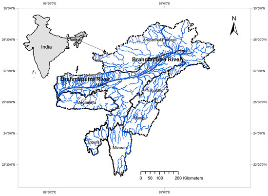
Figure 1.
Location map of the Brahmaputra River in Assam, India.
Two sets of Survey of India toposheets (1914 and 1975) and a set of IRS satellite photos encompassed the cloud-free time to study a portion of the Brahmaputra’s reach [2]. The area of Majuli Island has shrunk by 39.30 km2 in the Brahmaputra valley over the last 12 years [3]. Studies are being reported from time to time for a better understanding of the morphodynamics of the Brahmaputra River.
Braided River Modeling
Secondary flow structures associated with bed topography and water surface gradients exist in rivers that braid and are induced by planform changes. When there are considerable flow changes in cross-stream directions, such as those caused by flow curvature or turbulence, computational hydraulic analysis with topographic 1D modeling fails. As a result, 1D models may accurately predict the volume and timing of bank flow. However, when it comes to interest within reach flows with cross-stream flow changes, a 2D, if not a 3D, treatment is required [3,4].
Secondary flows exist in the plane perpendicular to the dominant flow’s axis. They are the result of interactions between primary flow and gross channel characteristics [5]. A vertical change in main flow velocity causes an imbalance between the transverse water surface gradient force and centrifugal forces over depth, resulting in a secondary transverse flow [3]. Most channel changes in braided rivers are linked to changes in bed morphology, which occur at high flows when observation is difficult [6]. Several attempts have been made to simulate the realistic flow field, including transverse components in complex geometry like bends and curves [5,7,8,9,10]. More recently, the hydrodynamic model has been used to represent the evolution mechanism of a meandering river [11]. However, the assessment of flow fields in braided rivers with ‘secondary flow correction’ in complex morphometry is yet to be fully understood. Many researchers have attempted to represent braided river morphodynamics to understand the physical processes involved. Braided channels do not explicitly originate simultaneously with the braided channel network, but rather through a protracted process of channel migration and avulsion [12]. It is observed that, due to the intricate system of channels and bar formation processes, there are significant local and transient changes in bedload transit rates. Recent advancements in image processing, sensor technology, and portable remote-sensing systems provide the opportunity to create terrain models with survey-quality data at a fraction of the cost and without the traditional deployment and logistical challenges. They studied distributed, depth-averaged flows in a broad, shallow, gravel-bed braided river using higher-dimensional hydrodynamic modeling. Digital elevation models (DEMs) created by utilizing optical bathymetric mapping and structure-from-motion on two linked stretches of the Ahuriri River in New Zealand formed the basis for the topography used in the simulations conducted [13]. These simulations reportedly facilitated a powerful demonstration of the suitability of terrain models for hydrodynamic applications. Similarly, in braided rivers, Ref. [14] investigated the morphodynamic impacts of rising yearly peak discharges. The chosen study site was a braiding stretch of the Upper Yellow River. They assessed the effects on floodplains, smaller-scale bars, channel branching, and the overall channel structure. From the model results, the influence of median grain size was found to have a negligibly small impact on the modeled channel pattern, which was found to be particularly sensitive to the parametrization of the bed slope effect [14]. Time-lapse images of the proglacial, gravel-braided Sunwapta River in Canada were used to evaluate planimetric change on daily hydrographs over two meltwater seasons [15]. The outcomes demonstrated the possible use of planimetric change measurements using time-lapse imaging as a low-cost, high-frequency monitoring tool for braiding dynamics and also as a stand-in for bedload transport measurement. Similarly, researchers further investigated the crucial role dunes play in regulating processes at the bar and channel scales, as well as river morpho-dynamics [16]. With implications for morphodynamic modeling, the findings of a numerical modeling and field monitoring study that were integrated to isolate the influence of dunes on depth-averaged and near-bed flow structures were presented. They concluded that models must take into account the impact of near-bed flow and sediment transport resulting from both dune- and bar-scale morphology. More recently, Ref. [17] published a study on the effects of climate change on the Qinghai–Tibet Plateau (QTP), which accelerated the melting of glaciers and caused significant changes in water and sediment flux in the Yangtze River’s Source Region (SRYR). The research provided insight into how braided rivers on the QTP are changing morphologically in response to runoff changes that are mostly brought on by climate change.
The transnational Brahmaputra River originates in China, flows through India, and eventually falls into the Bay of Bengal in Bangladesh. As stated earlier, the severe braiding, numerous laterals, mid-channel bars, and islands of this large river’s mid-reaches, which extend up to around 622 km, are located in the Assam flood plains of the northeastern region of Indian territory. Previous research on the Brahmaputra River relied significantly on field observations and physical modeling due to these features. Similarly, relations between stream power, braiding intensities, and bank erosion with a quantitative assessment of the spatiotemporal behavior of the channel braiding process in certain stretches of the Brahmaputra River were reported based on the spatial analysis of remote sensing images for the discrete years of 1990, 1997, and 2007 [18]. After the 1980s, numerical modeling, particularly 1D modeling, was extensively used in the Brahmaputra River for flow simulation and silt prediction. However, the actual use of 2D depth-averaged modeling in Brahmaputra River reaches in the Assam Plains is rare due to topographical difficulties and the difficulty of numerically replicating geometric data. Several attempts were made by researchers to transform and incorporate complex geometries into mathematical models for different but specific types of engineering problems. Some works, such as [19,20,21,22], can be referred to. According to [19], a continuum technique was attempted that used shock waves that were either captured or fitted. Although shock-capturing codes have straightforward algorithms, they frequently experience numerical issues, which become especially problematic when shocks are powerful and the grids are unstructured. They demonstrated how recent developments in computational mesh generation enable the alleviation of some of the challenges associated with shock capture and contribute to making shock fitting on unstructured meshes a versatile technique. The modeling and meshing of such a fractured network system are typically time-consuming and challenging due to the geometric complexity of the computational domain brought on by the existence and extension of fractures [20]. The method was reportedly applied to model two- and three-dimensional discrete fractured network (DFN) systems in geological problems to demonstrate its effectiveness and high efficiency. A three-dimensional manifold cutting program algorithm was developed by [21], and it can produce any three-dimensional manifold element under tetrahedral and hexahedral mesh covers. It can, however, result in numerical complexity and is restricted to smaller-scale flow regions. Researchers proposed a derivative-free mesh optimization algorithm, aiming to enhance the mesh’s worst element quality [22]. More recently, an analytical–numerical model for predicting the evolution of gravel bars in conditions of dynamic equilibrium was reported [23]. Numerical results showed that the proposed mesh optimization algorithm outperforms the existing mesh optimization algorithm in terms of improving the worst element quality and eliminating inverted elements on the mesh. There have been numerous attempts at complex mesh creation algorithms featuring complex geometries; nonetheless, mesh generation with complex morphometries and a very large-scale flow domain is still limited. In other words, efficient mesh generation for a highly complex river planform of a braided river with highly varied bed elevations, such as the Brahmaputra River, is hardly found in the literature.
Hence, this paper explores an attempt to develop a mathematical model for the highly complex planform of a braided river with a relatively realistic assessment of its geometric features. The model was then tested on a 100 km river stretch using a numerical 2D depth-averaged model with an improved flow dispersion stress tensor as an additional source term. To simulate the flow field, the model employs a finite-volume method with the SIMPLEC algorithm and Rhie and Chow’s momentum interpolation technique [24] on a curvilinear, non-staggered grid to solve non-homogeneous Poisson’s equations for boundary-fitted domain discretization. In order to simulate the river’s braiding process, the wetting and drying process [10] was added to the model.
2. Materials and Methods
2.1. Grid Generation Algorithm
The governing differential equations for engineering problems are derived and expressed in a Cartesian (rectangular) coordinate system. We must discretize the continuous physical space into a uniform orthogonal computational space to solve these differential equations [25]. A detailed flow chart is presented in Figure 3.
However, the applications of boundary conditions require that the boundaries of the physical space fall on the coordinate lines (surfaces) of the coordinate system. Furthermore, accurate solutions necessitate that grid points be dispersed in small-gradient regions and clustered in large-gradient regions. The general procedure adopted for grid generation was widely referred from [25]. For mapping the body-fitted, non-uniform physical plane (x, y, t) onto the transformed uniform orthogonal computational plane (ϕ, ψ, t), the following elliptic PDE (Poisson’s equation) was used for grid generation.
where and are non-homogeneous terms. Coordinates () are known and () are not known. The objective of the grid generation process is to determine the grid in the x, y space. The inverse transformation is
One can obtain the transformed equations in following condensed form as
where, , , ; , , ,, .
Furthermore, for the orthogonal condition [21], one has .
2.1.1. Numerical Discretization and Algorithm
These are elliptic PDEs with Dirichlet boundary conditions. Writing the equation in finite-difference form using second-order centered-difference approximations of the exact partial derivatives, one may obtain the following final numerical equations (based on finite-difference grid shown in Figure 2) (considering ):
For x direction:
For y-direction:
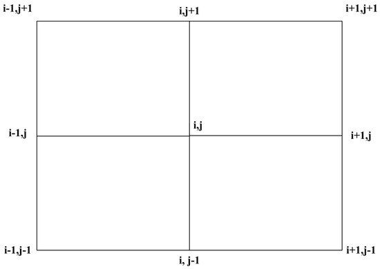
Figure 2.
Finite-difference grid for discretization at node P.
Using the ADI (Alternating-Direction Implicit–Explicit) scheme, one can obtain Equations (5a) and (5b) in tridiagonal matrix form for unknowns (row-wise):
Similarly, one can obtain Equations (6a) and (6b) in tridiagonal matrix form (column-wise):
- (a)
- Convergence Criteria
Iteration continues until the following condition is fulfilled:
where is the number of iterations.
Using appropriate terminologies, Equations (5a) and (5b) can be written in the following format.
At the th iteration,
where is evaluated on the latest best-known values of x and y and , .
One can compute intermediate variables (TDMA) to obtain the solution. The solution in steps are as follows: (i) assign a number of boundaries and constraints; (ii) select the corresponding degree of polynomial; (iii) generate simultaneous equations of Ai, Bi, Ci, Oi, Pi, and so on by putting boundary values in polynomial equations; (iv) solve simultaneous equations through matrix inverse multiplication for Ai, Bi, Ci, and Pi; (v) using polynomials, determine the value of x for corresponding integer values in the range of (fixed by the user appropriately to obtain the desired mesh resolution); (vi) evaluate the corresponding values of y from cubic interpolation of the curve data; (vii) the same procedure is adopted if the boundary is aligned by and large along the y axis. One can refer the detailed flow chart as shown in Figure 3.
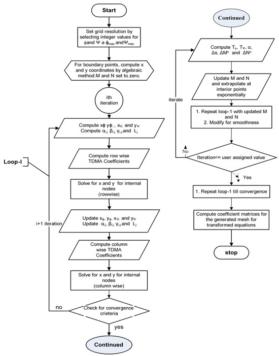
Figure 3.
Flow chart of grid generation algorithm.
2.1.2. Numerical Computation of Non-Homogeneous Terms
- (a)
- Interior grid point control.
Poisson’s equation that is used in grid generation essentially contains non-homogeneous terms M and N. The finite-difference forms also naturally contain these terms. To optimize orthogonality, one must choose specific functional forms to control the interior grid points to the desired level of their distribution [25]. The literature has found numerous numerical approaches to address this specific problem. For detail, readers may refer to [26,27,28]. The technique for implementing the interior grid control was implemented in [28], although it is not absolute. It is an iterative approach that is quite comfortably implemented to evaluate M(ϕ, ψ) and N (ϕ, ψ). After the values are determined at the boundaries, interior values are extrapolated exponentially to achieve the desired effect in the interior grid points as follows:
Initially, M (ϕ, ψ) and N (ϕ, ψ) are not known. So, the initial values of M and N are set to zero and Poisson’s equation is solved to obtain interior points and updated recursively while evaluating M and N for each iteration as follows:
Let us say that at the nth iteration, M and N are and .
So, at the n + 1th iteration, the new values of M and N will be
n denotes the iteration level. The initial values of M and N are set to zero.
Let us define some terminologies:
= Tangent vector to the -line at the boundary. = Tangent vector to the -line at the boundary. The dot product will give the angle between tangent vectors.
One then has
Let α* be the desired angle of intersection. Then, the required correction to is
To make the line orthogonal to α*, is taken. The spacing ΔS between the boundary point and the first interior point on the line is given by
Let be the desired spacing; then, the required correction to is
ΔS* may be set as per the domain resolution or may conveniently be taken by the user as the smallest permissible spacing of the domain between the boundary point and the first interior point on the ϕ-line. Either or both of the corrections ΔMn. and ΔNn. can be over-relaxed or under-relaxed.
- (b)
- Top boundary implementation.
For the top boundary, one can calculate and as follows:
where and are unit vectors along the x and y axis. and can be determined as follows:
After computing and , one can compute from Equation (10b) and from Equation (11). Using the value of from Equation (15), is computed. Then, M and N for the next step are updated.
- (c)
- Bottom boundary implementation.
For the bottom boundary, one can calculate and as follows:
where and are unit vectors along the x and y axis. and can be determined as follows:
After computing and , one can compute from Equation (10b) and from Equation (11). Using the value of from Equation (19), is computed. Then, M and N for the next step for the bottom boundary are updated.
- (a)
- Extrapolation of boundary values to interior points.
Extrapolation of the boundary values of and (,) into interior points of the domain is performed to achieve the desired effect in the interior grid points. For this, exponential extrapolation is adopted herein [25].
where the first term represents the boundary control on the bottom boundary and the second term represents the boundary control on the top boundary. A large value of the exponential term gives rapid decay and vice versa. In this model, the adopted values of coefficients were 9.0. Similarly, for downstream, upstream boundaries M and N were evaluated and extrapolated. M and N were averaged to include the effect of all four boundaries of the domain.
- (e)
- Improved mesh generation system.
A good balance of orthogonality and smoothness without distortion and overlapping is represented in the method proposed by [29], which was applied by introducing the effect control factor on non-homogeneous terms M and N as follows.
For each grid point factor, (1−rm) and (1−rn) were applied to the terms M and N to obtain improved M and N for incorporation of smoothness as
In Equations (9a) and (9b),
where and are improved terms, and and are locally averaged scale factors along the and directions.
2.1.3. Quality of the Generated Grid
There are three indices to evaluate the quality of a mesh system: uniformity, orthogonality, and adaptivity [29]. Uniformity indicates how uniform the mesh spacing is; orthogonality is a measure of to what extent the mesh lines are perpendicular to each other; and adaptivity indicates the degree of the mesh density distributed in areas where higher resolution and accuracy are desired. These are measured by the following functions:
where Iw, Is, and Io are measures for adaptivity, uniformity, and orthogonality, respectively. The Jacobian I represent the area of a mesh cell in two dimensions and is the weighing factor. When this integral is minimized, (with ) should have a uniform distribution, so when the weighting function is large, the mesh size should be small. The weighting function is often formulated using water depth or bed bathymetry to handle complex hydrodynamic problems. If the numerical solutions such as the concentration or the velocity gradients are selected, the mesh shall be adaptive dynamically with the numerical solution [29]. The factor is added to enforce the orthogonality with higher weighting for large cells in Equation (11c). If the three indices approach their minimum values, the mesh would have the optimal combination of uniformity, orthogonality, and adaptivity. In general, a mesh can be generated by minimizing the sum of the three integrals with a relative weighing factor with each integral. Since it is impossible to achieve optimized weighing factors at the same time, for a particular mesh, one needs to select the appropriate combination of these coefficients. In this study, orthogonality was emphasized more than other indices for the numerical ease of hydrodynamic solution. It should be mentioned here that topographical variations were irregular and large, and the mesh used in this study was of fixed domain. Hence, optimizing indices like adaptivity and uniformity may increase complications in obtaining feasible mesh generation with nearly orthogonal grids.
2.1.4. Mesh Evaluation
Several indices to quantitatively evaluate mesh quality by several indicators were suggested [29]. These were the Maximum Deviation Orthogonality (MDO), Averaged Deviation from Orthogonality (ADO), Maximum Aspect Ratio (MAR), and average grid aspect ratio (AAR), as given in the following equations:
where and are the maximum number of mesh lines in the and directions, respectively; and is defined as
For the generated mesh to be perfectly orthogonal, ADO and MDO should be 1.57(π/2). For a perfectly smooth mesh, MAR and AAR should be the same.
2.1.5. Computation of Coefficient Matrices for the Generated Curvilinear Mesh
Difference formulas for derivatives were developed to compute coefficient matrices, which are various derivatives or combinations of derivatives between independent variables x and y with ϕ and ψ depending upon the availability of neighborhood nodes.
C++ computer code was developed using the finite-difference method with the algorithm presented in the previous section, and it was coupled with the flow simulation numerical scheme to facilitate a prime input for domain geometry variables and coordinate transformation coefficients to be used in the governing equations for flow simulation on the boundary-fitted domain. Arbitrarily chosen curvilinear domains with known boundary coordinates and mesh evaluation are presented in Figure 4 from the developed computer code.
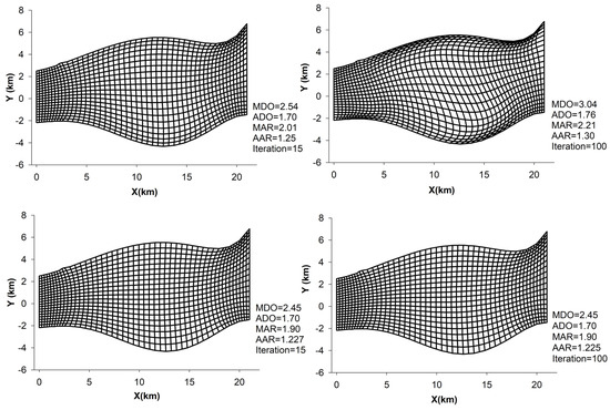
Figure 4.
Mesh generation for a given curvilinear domain using the developed C++ code.
2.2. Depth-Averaged Flow Model
The governing equations are RANS (Reynolds-averaged Navier–Stokes) equations with a depth-averaged approximation of continuity and momentum equations (Equations (28a)–(28c)) in the Cartesian coordinate system [30].
where and are depth-averaged velocity components in the x and y directions; t is time; is the density of water (kg/m3); H is water surface elevation; h is the depth of the flow; g is the acceleration of gravity; f is the frictional stress coefficient (for friction shear stress at the bottom in the x and y directions) and is with n = Manning’s coefficient and = eddy viscosity. The components of dispersion stress terms in Cartesian coordinates which can be included in momentum transport equations are , , and . These terms can be expressed as follows [31,32]:
where z0 is the zero-velocity level.
Cohesive terms are insignificant in an open-channel free-surface gravity flow and can be ignored. For the turbulence term, the depth-averaged parabolic eddy viscosity model (zero-equation model) is used. Equation (30) estimates the depth-averaged eddy viscosity.
where is the von Karman’ coefficient and V* (Shear velocity) = .
The transformed governing equations in the curvilinear coordinate system (, , τ) (Equations (31a)–(31c)) are derived as follows [33]:
In Equations (31a)–(31c), ( = ϕ, ψ) are the components of velocity in the curvilinear coordinate system (,,) which are related to Vx, Vy as
Numerical Solution
The finite volume method was used to discretize the controlling partial differential equations described in the previous section on a curvilinear, non-staggered grid. In the curvilinear coordinate system, the mass and momentum equation may be stated in conservative tensor notation. Readers can refer to [33] for the complete numerical scheme to solve the above sets of equations with implemented boundary conditions.
3. Mathematical Representation of Complex Morphometry: Study River Reach
For application of the developed hydrodynamic model, the reach between measured cross-section numbers 22 (location at Pandu near Guwahati) and 9 (Jogighopa) released by the Brahmaputra Board, Government of India (spanning over about 100 km in the state of Assam in Indian Territory), was chosen as the flow domain and extracted from a satellite image of the study reach. Fourteen measured cross-section data points (cross-section 22 to cross-section 9) for the year of 1997 were used. The location of the study reach of the Brahmaputra River is shown in Figure 5. The flow domain (Primary Flood Plain) of the study area is delineated from a geo-referenced satellite image (IRS-LISS-III satellite imagery) from 1997 using GIS tools. Figure 5 displays the delineated image of the river’s study reach. Figure 6 depicts the geo-referenced image of the extracted flow domain for further pre-processing.
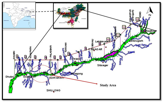
Figure 5.
Location map of the study area.
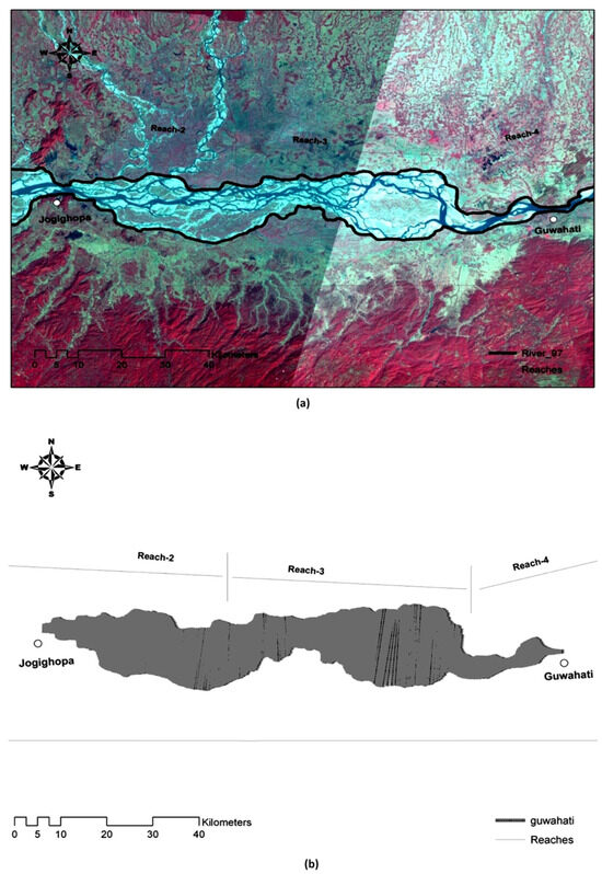
Figure 6.
Delineated study area from satellite image. (a) Adapted with permission from reference [33]. Copyright 2024, Springer, Singapore. (b) Reprinted with permission from reference [33]. Copyright 2024, Springer, Singapore.
Along the Brahmaputra River, there are three to four restricted nodal sites where the cross-sections remain constant in time and space. Therefore, due to its division by well-defined nodal points (with invariant width), the Brahmaputra reach presents a relatively simple 2D mathematical model application for both upstream and downstream border implementations. The existence of various 3D flow structures inside the flow domain makes the process of modeling a fully evolved braided stream a difficult undertaking. This analysis was conducted using data sets for a river stretch with two restricted nodal points, namely Pandu and Jogighopa, of roughly 100 km in reach length of the Brahmaputra River, with fourteen measured river cross-sections and 1997 hydrological data points.
3.1. Hydrographic Data
As stated, domain boundaries (main channel and largely low flood plain) for the study period were extracted in a geographical coordinate system from the remote sensing imagery shown in Figure 6 and transformed into a Cartesian coordinate system to accurately represent the domain in the Cartesian plane (Figure 7). The main waterway, low flood plains, and high flood plains were all cross-sectioned. Some segments within the river study stretch have dikes built for flood protection purposes. Poor maintenance often leads to breaches in these dikes during high-flood seasons. Low- and medium-flood periods result in inundation of the main channel and low flood plains. Keeping this in view, care was taken to extract the flow domain to include the primary flood plain, and then cross-sections were fitted.
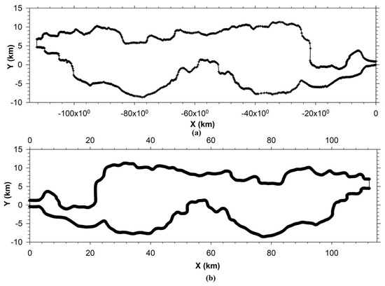
Figure 7.
Domain in (a) transformed coordinate system and (b) reorientation in positive x-direction with upstream nodal point as origin.
The bank lines were delineated on a geo-referenced image covering the river reach in the year of 1997 through identifying river sandy bed fringes with vegetative cover along the bank lines. The coordinate system of the geo-referenced image was WGS 84 (Word Geodetic System 1984). Thus, x and y of the boundary grid points were obtained.
Additionally, boundary grid points were uniformly redistributed using an algebraic approach into 451 points along the positive x-axis (south and north limits) and 51 points along the y-axis. For convenience of sign convention, the domain was re-oriented with the positive x-axis aligned with the flow direction. Some of the extreme grid points upstream and downstream of the flow domain were corrected and rectified to fit the measured cross-section in the given orientation, which may have crept in due to a manual digitization error. Boundaries were slightly smoothed through a three-point finite Fourier transform (FFT) using math-processing software to generate an efficient mesh without changing the basic characteristics of the domain (Figure 7).
The reduced levels of the river cross-sections of the post-monsoon period for the year of 1997 were collected for all fourteen pre-defined river cross-sections from the Brahmaputra Board, Government of India. The positioning of the measured cross-sections and mid-central line (in blue) into the domain is represented in Figure 8 and are depicted in graphical form in Figure 9. The data were normalized. The bearing at cross-section 22 (C/s-22) was zero and was the physically identified position on the imagery used to extract the domain. Taking reference to C/S-22, cross-sections could be positioned and oriented if chainage and bearing were known. To characterize the flow-carrying capacity of a stream and its associated floodplain, measured cross-sections were placed at intervals along the stream as per their orientations. They extended across the entire floodplain and were perpendicular to the anticipated flow lines. Every effort was made to obtain interpolated stream bed data at mesh nodes based on these measured cross-sections so that the data would accurately represent the stream and floodplain geometry. The adopted process of bed interpolation appropriate for the available data set is discussed in subsequent sections.
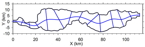
Figure 8.
Positioning of measured cross-sections and mid-central line (in blue color) into the domain.
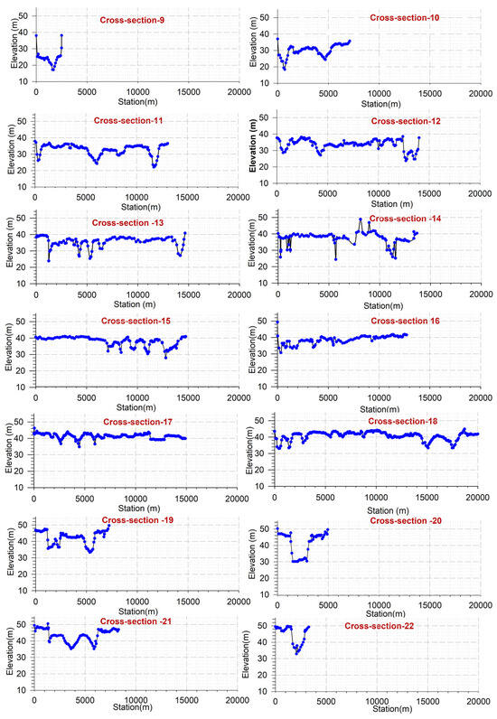
Figure 9.
Measured cross-sectional data points for reach cross-sections of the study reach.
As discussed earlier, cross-sections were fit at the position and bearing as per Table 1. The measured cross-sectional data from the left bank of the river were normalized, and 101 points were extracted through the linear interpolation technique to obtain nodal points for a structured matrix for bed interpolation, discussed in the subsequent section.

Table 1.
Study reaches of Jogighopa–Pandu of Brahmaputra River.
3.2. Stream Bed Interpolation
Stream bed interpolation is a way to add bed elevations from a topology or bathymetrical database to mesh nodes. Several methods and algorithms are available in the literature. For the type of observed data available, the Inverse Distance Weighing (IDW) method with a structured database was applied as described by [29]. Refinement was performed by normalizing and expanding to desired data points in the transverse direction along each cross-section using linear interpolation. Thereafter, each cross-section was divided into three parts, left over bank (LoB), main channel, and right over bank (RoB), appropriately as per the cross-section configuration. An equal number of points in these three parts was distributed. Furthermore, the database in the longitudinal direction between cross-sections was normalized and expanded to the desired data points between cross-sections. Linear interpolation was used between the corresponding parts of each cross-section to obtain interpolated data points. Adopting this procedure, a ‘structured matrix’ of data points from the measured data points was generated. Now, from the quadrilateral formed from these matrix elements, each grid points to be interpolated was identified, and using the IDW method, bed elevation was determined for known x and y coordinates. As discussed above, the cross-section was positioned and oriented as per the chainage and bearing given in Table 1, numbered from cross-section 9 (downstream) to 22 (upstream) in Figure 8. Out of the measured data for each cross-section, data were normalized, and 101 equally distanced data points were extracted for each cross-section.
From the normalized data point of each cross-section, 21 data points were linearly interpolated for each set of two adjacent cross-sections through HEC-RAS (Hydrological Engineering Center-River Analysis System) geometric interpolation application software [34] to interpolate the data along the deepest bed level, ensuring flow continuity in the main channel. Thus, a structured matrix of dimension 101 × 261 data points was generated. It is presented graphically in Figure 10a, and the corresponding contour plot of bed-elevation is presented in Figure 10b.
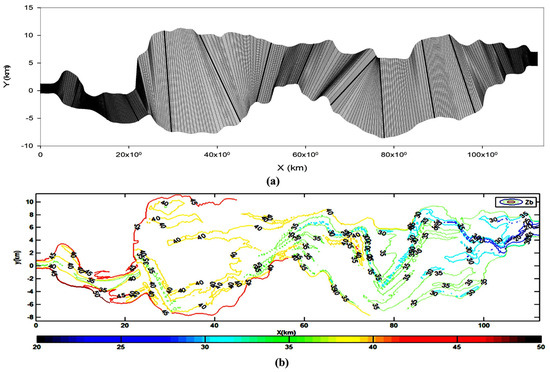
Figure 10.
(a) Data points and (b) contour plot of structured matrix.
Discretization of the domain was performed through the developed computer code (Figure 11a) using the method described in the previous section, and a bed-level matrix (51 × 451) was generated using the IDW (Inverse Distance Weighting) method. Bed interpolation was also performed for discretized array [x, y] using the MATLAB tool using the ‘nearest neighborhood technique’ for comparing and checking the accuracy of the interpolated bed elevation using the IDW method. Data generated by the IDW method did contain some localized discrepancies in comparison to the ‘nearest neighborhood technique’ as generated from MATLAB code. Hence, a MATLAB-generated matrix was preferred and is presented in Figure 11b as a contour map with interpolated bed elevation, further presented in Figure 12 as a 3D view for clarity. Thus, the flow domain was discretized, and an appropriate digital terrain model with a chosen meshing array and fineness was generated.
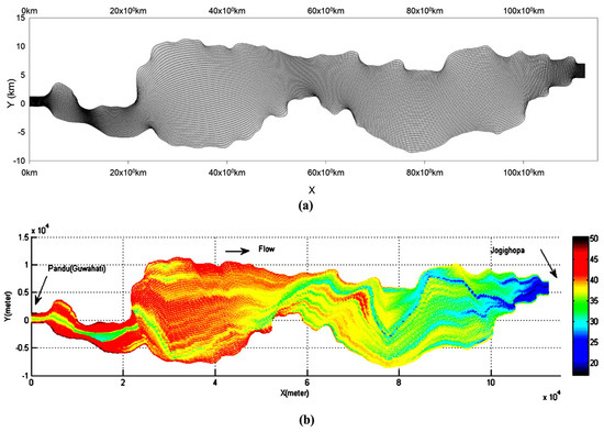
Figure 11.
(a) Domain discretization in Cartesian coordinate system. (b) Interpolated bed-elevation for study domain using MATLAB code. (Reprinted subfigure (a) (adapted) with permission from reference [33]. Copyright 2024, Springer, Singapore.)
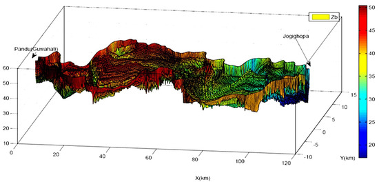
Figure 12.
Three-dimensional surface plot of generated bed level of the flow domain (bed level in m).
4. Results and Discussion
The hydrologic data are composed of water discharges and flow durations. The discharge hydrograph is approximated by a sequence of steady inflow discharges, each of which occurs for a specified number of days or hours, depending upon the acquisition of data. Water surface profiles are computed by using the 2D depth-averaged mass momentum equations.
The river geometry of the study stretch is reproduced mathematically using the available observed field cross-sectional data. Bed interpolation is performed mathematically to determine the bed elevation at each grid point of the generated mesh for the study flow domain, which is otherwise impossible to acquire from the field for grid points with such a fine grid spacing in both stream-wise and transverse directions.
The developed grid generation for the complex geometry of Brahmaputra River was successfully tested and verified using the 2D depth-averaged improved hydrodynamic model underlined in Section 2.2. The Brahmaputra follows an aligned channel arrangement throughout this study. Long stretches of the river have a three-dimensional flow that is practically unsteady. Simulating the 2D flow for such a long reach with widths ranging from 2 km to 22 km requires a large amount of data. The data required to model unsteady flow in 2D for a large alluvial river like the Brahmaputra are difficult to come by. Nonetheless, a steady flow simulation utilizing a 2D model for a large alluvial river gives valuable information and a sufficient grasp of actual flow conditions for practical engineering applications. Comparing observed water levels at Pandu (upstream node) with model-simulated water levels for the implemented stage discharge rating curve at the downstream node was utilized to validate the model.
In channels characterized by sloping banks, sandbars, and islands, the water’s boundary undergoes continual change over time, potentially leaving portions of the area exposed. Various strategies have been documented in the literature to address this issue. One such approach is the utilization of a ‘fixed grid’ method, which encompasses the largest submerged area (primary floodplain) and considers dry regions as part of the computational domain [10]. This method incorporates the ‘small imaginary depth’ technique, which employs a minimum flow depth threshold (e.g., 0.02 m in natural waterways and 0.001 m in controlled flumes) to determine the presence of dry or wet conditions at each time interval. Dry regions are assigned zero velocity, and the interface between dry and wet zones is treated as an internal boundary where the wall function methodology is applied. Similarly, the dry zones in the flow domain were simulated for various flow discharges using the wetting and drying technique.
The wetting and drying technique was incorporated to judge whether an individual grid was wet or dry by assigning a threshold depth of 0.02 m. In the pressure solver, all wet and dry grids participated in the solution. While computing water surface elevation, the H value of those nodes where the computed WSL was less than or equal to the bed elevation (i.e., H ≤ zb) was assigned a numerical threshold value of 0.02 m for solving momentum equations. In the final results, for practical purposes, H values of 0.02 or less were considered dry nodes with a water depth assigned to zero. Figure 13 shows the correlation of WSL for upstream location and discharge for downstream location when compared with the observed values suggesting the accuracy and validation. Figure 14 depicts the dry zones with zero water depth in black hues. Looking at Figure 14, it was observed that braiding intensity increased with decreasing discharges, and more and more braid bars and side bars evolved, thereby increasing the proportionate flow zone in the flow domain. Even though the flow-fields at channel bifurcations are essentially three-dimensional, the developed model with a computer-generated flow domain was able to approximate braid bars or side bars with reasonable accuracy through implementing wetting and drying techniques without developing a numerically more expensive 3D model for such a macro-scale flow field scenario.
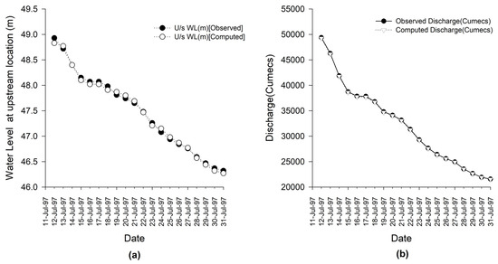
Figure 13.
(a) Observed versus computed WSL plot for u/s location (b) discharge for d/s location for the study reach of Brahmaputra River during receding flood of the year of 1997. (Reprinted (adapted) with permission from reference [33]. Copyright 2024, Springer, Singapore.)
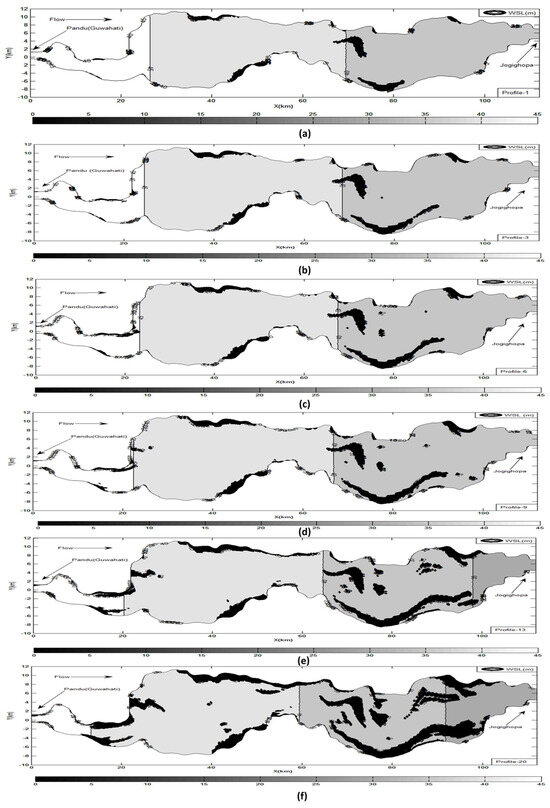
Figure 14.
(a–f) Model-simulated braid bars/side bars of the study reach with receding flood. (d–f) Reprinted (adapted) with permission from reference [33]. Copyright 2024, Springer, Singapore.
5. Conclusions
- This work establishes a stepwise, freshly developed procedure and algorithm to mathematically evolve mathematic-fit boundary-fitted bathymetric mesh generation with quality and chosen fineness for a braided river flow domain with highly complex morphometric structures with realistic assessment to create intensive geometric data for multidimensional river flow/sediment transport modeling with bank erosion and morphological changes.
- A realistic assessment of bank erosion and riverbed development/braid bars for alluvial rivers could be conducted using enhanced and realistic flow-field estimates and secondary flow correction in terms of dispersion stress tensors and developed morphometric data as major inputs. Braiding was found to intensify when the incoming discharge into the reach diminishes over time.
Author Contributions
Conceptualization, M.P.A. and C.S.P.O.; methodology, M.P.A. and C.S.P.O.; validation, M.P.A., C.S.P.O. and N.S.; formal analysis, M.P.A.; investigation, M.P.A., C.S.P.O. and N.S.; resources, data curation, N.S. and M.P.A.; writing—original draft preparation, M.P.A., P.S. and S.K.; writing—review and editing, M.P.A., P.S. and S.K.; visualization, M.P.A. and C.S.P.O.; supervision, C.S.P.O. and N.S. All authors have read and agreed to the published version of the manuscript.
Funding
This research received no external funding.
Data Availability Statement
The data presented in this study are available on request from the corresponding author.
Acknowledgments
The National Disaster Management Authority of India (NDMA, Govt. of India), New Delhi, provided some of the specific field data used in this study, which is graciously acknowledged here. During the preparation of this work, the author(s) used MATLAB (Matrix Laboratory) and HEC-RAS (Hydrological Engineering Center-River Analysis System) tools in order to analyze morphometric data of Brahmaputra River. After using this tool, the authors reviewed and edited the content as needed and are graciously acknowledged for the same for using abovementioned packages.
Conflicts of Interest
The authors declare no conflicts of interest.
References
- WAPCOS. Morphological Studies of River Brahmaputra; WAPCOS: New Delhi, India, 1993. [Google Scholar]
- Kotoky, P.; Bezbaruah, D.; Baruah, J.; Sarma, J.N. Nature of Bank Erosion along the Brahmaputra River Channel, Assam, India. Curr. Sci. 2005, 88, 634–640. [Google Scholar]
- Sankhua, R.N. ANN Based Spatio-Temporal Morphological Model of the River Brahmaputra. Ph.D. Thesis, Department of Water Resources Development & Management, Indian Institute of Technology Roorkee, Uttarakhand, India, 2005. [Google Scholar]
- Bates, P.D.; Lane, S.N.; Ferguson, R.I. Computational Fluid Dynamics: Applications in Environmental Hydraulics; Wiley & Sons: Hoboken, NJ, USA, 2005; ISBN 978-0-470-84359-8. [Google Scholar]
- Seo, I.W.; Lee, M.E.; Baek, K.O. 2D Modeling of Heterogeneous Dispersion in Meandering Channels. J. Hydraul. Eng. 2008, 134, 196–204. [Google Scholar] [CrossRef]
- Smith, N.D. The Braided Stream Depositional Environment: Comparison of the Platte River with Some Silurian Clastic Rocks, North-Central Appalachians. GSA Bull. 1970, 81, 2993–3014. [Google Scholar] [CrossRef]
- Lien, H.C.; Hsieh, T.Y.; Yang, J.C.; Yeh, K.C. Bend-Flow Simulation Using 2D Depth-Averaged Model. J. Hydraul. Eng. 1999, 125, 1097–1108. [Google Scholar] [CrossRef]
- Majumdar, S.; Rodi, W.; Zhu, J. Three-Dimensional Finite-Volume Method for Incompressible Flows with Complex Boundaries. J. Fluids Eng. 1992, 114, 496–503. [Google Scholar] [CrossRef]
- Odgaard, A.J. River-Meander Model. I: Development. J. Hydraul. Eng. 1989, 115, 1433–1450. [CrossRef]
- Wu, W. Computational River Dynamics; CRC Press: London, UK, 2007; ISBN 978-0-429-22428-7. [Google Scholar]
- Liu, L.; Zhu, H.; Huang, C.; Zheng, L. Evolution Mechanism of Meandering River Downstream Gigantic Hydraulic Project I: Hydrodynamic Models and Verification. Math. Probl. Eng. 2018, 2018, e5980609. [Google Scholar] [CrossRef]
- Ashmore, P. 9.17 Morphology and Dynamics of Braided Rivers. In Treatise on Geomorphology; Shroder, J.F., Ed.; Academic Press: San Diego, CA, USA, 2013; pp. 289–312. ISBN 978-0-08-088522-3. [Google Scholar]
- Javerick, L.; Hicks, D.M.; Measures, R.; Caruso, B.; Brasington, J. Numerical Modelling of Braided Rivers with Structure from Motion Derived Terrain Models. Available online: https://onlinelibrary.wiley.com/doi/abs/10.1002/rra.2918 (accessed on 7 February 2024).
- Schuurman, F.; Ta, W.; Post, S.; Sokolewicz, M.; Busnelli, M.; Kleinhans, M. Response of Braiding Channel Morphodynamics to Peak Discharge Changes in the Upper Yellow River. Earth Surf. Process. Landf. 2018, 43, 1648–1662. [Google Scholar] [CrossRef]
- Middleton, L.; Ashmore, P.; Leduc, P.; Sjogren, D. Rates of Planimetric Change in a Proglacial Gravel-Bed Braided River: Field Measurement and Physical Modeling. Earth Surf. Process. Landf. 2018, 44, 752–765. [Google Scholar] [CrossRef]
- Unsworth, C.A.; Nicholas, A.P.; Ashworth, P.J.; Best, J.L.; Lane, S.N.; Parsons, D.R.; Sambrook Smith, G.H.; Simpson, C.J.; Strick, R.J.P. Influence of Dunes on Channel-Scale Flow and Sediment Transport in a Sand Bed Braided River. J. Geophys. Res. Earth Surf. 2020, 125, e2020JF005571. [Google Scholar] [CrossRef]
- Lu, H.; Li, Z.; Hu, X.; Chen, B.; You, Y. Morphodynamic Processes in a Large Gravel-Bed Braided Channel in Response to Runoff Change: A Case Study in the Source Region of Yangtze River. Arab. J. Geosci. 2022, 15, 377. [Google Scholar] [CrossRef]
- Akhtar, M.P.; Sharma, N.; Ojha, C.S.P. Braiding Process and Bank Erosion in the Brahmaputra River. Int. J. Sediment Res. 2011, 26, 431–444. [Google Scholar] [CrossRef]
- Bonfiglioli, A.; Paciorri, R.; Di Mascio, A. The Role of Mesh Generation, Adaptation, and Refinement on the Computation of Flows Featuring Strong Shocks. Model. Simul. Eng. 2012, 2012, e631276. [Google Scholar] [CrossRef]
- Sun, S.; Sui, J.; Chen, B.; Yuan, M. An Efficient Mesh Generation Method for Fractured Network System Based on Dynamic Grid Deformation. Math. Probl. Eng. 2013, 2013, e834908. [Google Scholar] [CrossRef]
- Li, H.F.; Zhang, G. Researches on the Generation of Three-Dimensional Manifold Element under FEM Mesh Cover. Math. Probl. Eng. 2014, 2014, e140180. [Google Scholar] [CrossRef]
- Kim, J.; Shin, M.; Kang, W. A Derivative-Free Mesh Optimization Algorithm for Mesh Quality Improvement and Untangling. Math. Probl. Eng. 2015, 2015, e264741. [Google Scholar] [CrossRef]
- Pannone, M.; Vincenzo, A.D. Theoretical Investigation of Equilibrium Dynamics in Braided Gravel Beds for the Preservation of a Sustainable Fluvial Environment. Sustainability 2021, 13, 1246. [Google Scholar] [CrossRef]
- Rhie, C.; Chow, W. A Numerical Study of the Turbulent Flow Past an Isolated Airfoil with Trailing Edge Separation. In Proceedings of the 3rd Joint Thermophysics, Fluids, Plasma and Heat Transfer Conference, Fluid Dynamics and Co-Located Conferences, St. Louis, MO, USA, 7–11 June 1982; American Institute of Aeronautics and Astronautics: Reston, VA, USA, 1982. [Google Scholar]
- Hoffman, J.D. Numerical Methods for Engineers and Scientists, 2nd ed., Rev. expanded.; Marcel Dekker: New York, NY, USA, 2001; ISBN 978-0-8247-0443-8. [Google Scholar]
- Thomas, P.D.; Middlecoff, J.F. Direct Control of the Grid Point Distribution in Meshes Generated by Elliptic Equations. AIAA J. 1980, 18, 652–656. [Google Scholar] [CrossRef]
- Steger, J.L.; Sorenson, R.L. Use of Hyperbolic Partial Differential Equations to Generate Body Fitted Coordinates; NASA: Washington, DC, USA, 1 January 1980. [Google Scholar]
- Hilgenstock, A. A Fast Method for the Elliptic Generation of Three-Dimensional Grids with Full Boundary Control. Numer. Grid Gener. Comput. Fluid Mech. 1988, 1988, 137–146. [Google Scholar]
- Zhang, Y.; Jia, Y. CCHE2D Mesh Generator User’s Manual–Version 2.6; National Center for Computational Hydroscience and Engineering: Oxford, MS, USA, 2005. [Google Scholar]
- Duan, J.G. Simulation of Flow and Mass Dispersion in Meandering Channels. J. Hydraul. Eng. 2004, 130, 964–976. [Google Scholar] [CrossRef]
- Kalkwijk, J.P.T.; De Vriend, H.J. Computation of the Flow in Shallow River Bends. J. Hydraul. Res. 1980, 18, 327–342. [Google Scholar] [CrossRef]
- Zhu, J.; Rodi, W. A Low Dispersion and Bounded Convection Scheme. Comput. Methods Appl. Mech. Eng. 1991, 92, 87–96. [Google Scholar] [CrossRef]
- Sharma, N.; Akhtar, M.P. Prospects of Modeling and Morpho-Dynamic Study for Brahmaputra River. In River System Analysis and Management; Sharma, N., Ed.; Springer: Singapore, 2017; pp. 189–209. ISBN 978-981-10-1472-7. [Google Scholar]
- Brunner, G.W. HEC-RAS River Analysis System: Hydraulic Reference Manual; Hydrologic Engineering Center: Davis, CA, USA, 1997. [Google Scholar]
Disclaimer/Publisher’s Note: The statements, opinions and data contained in all publications are solely those of the individual author(s) and contributor(s) and not of MDPI and/or the editor(s). MDPI and/or the editor(s) disclaim responsibility for any injury to people or property resulting from any ideas, methods, instructions or products referred to in the content. |
© 2024 by the authors. Licensee MDPI, Basel, Switzerland. This article is an open access article distributed under the terms and conditions of the Creative Commons Attribution (CC BY) license (https://creativecommons.org/licenses/by/4.0/).