1. Introduction
Groundwater is a critical natural resource that helps sustain billions of livelihoods across the globe. Rapid urbanization, increased population growth, and climate change have strained several important aquifers across the world [
1,
2,
3]. Moreover, effective groundwater management is a crucial global issue that has far-reaching effects across multiple domains.
Over the past two decades, there has been a significant increase in the application of machine learning (ML) techniques in groundwater modeling. Researchers have utilized ML models to forecast groundwater quality indices and water table elevations with notable success [
4,
5]. A diverse array of ML algorithms, encompassing artificial neural networks (ANNs), fuzzy logic, autoregressive models, and support vector machines, has been employed in groundwater studies [
6,
7,
8]. These models demonstrate a promising capacity for generating reasonable numerical representations of groundwater systems, facilitating informed water management and decision-making processes.
However, comprehensive in situ groundwater level data are lacking in many regions. Thus, the ability to implement ML models for groundwater management is limited. Consequently, the development of simulation tools capable of accurately approximating realistic groundwater levels in the absence of extensive real data could be valuable.
Synthetic time series data have proven to be an invaluable resource in various domains, allowing researchers and practitioners to address challenges arising from limitations in data availability, quality, or confidentiality [
9]. In finance, synthetic time series data have been used to simulate stock prices or exchange rate fluctuations, facilitating the development and testing of trading algorithms, risk management strategies, and forecasting models without exposing them to real market data [
10]. In hydrology, synthetic rainfall data have been generated to assess the performance of watershed models or flood prediction systems under a range of meteorological conditions, ensuring robustness and reliability in real-world applications [
11,
12,
13].
In meteorology, synthetic weather data generators have been applied in studies related to climate change impact assessments, risk analysis, water resource management, agricultural planning, and renewable energy forecasting [
14]. These generators produce realistic weather scenarios based on historical data, enabling researchers and decision-makers to evaluate potential outcomes and implications under various conditions or policies. In the energy sector, synthetic data representing electricity consumption or renewable energy production have been used to optimize power grid management, evaluate the impact of different demand scenarios, or assess the feasibility of integrating renewable sources into existing infrastructure [
15,
16].
Furthermore, in the healthcare domain, synthetic time series data mimicking vital signs or physiological parameters have been employed to train machine learning algorithms for early diagnosis or anomaly detection, circumventing privacy and ethical constraints associated with real patient data [
17,
18].
Despite the widespread use of synthetic time series data in various fields, there is a significant lack of research on generating synthetic data related to groundwater management [
19]. This research paper aims to address this gap by presenting a novel method for generating synthetic groundwater levels using advanced ML techniques. The ability to generate realistic synthetic well data has the potential to significantly enhance the understanding and management of groundwater resources. This approach will enable the development of effective strategies for sustainable groundwater management and planning, even in regions constrained by limited observational data. Moreover, this approach will bolster the capacity of researchers to refine their current methods, improving the quantification of uncertainties, model validation, and calibration, leading to more informed decision-making in groundwater management (
Figure 1).
1.1. Overview of Existing ML Models for Generating Synthetic Time Series
The application of ML models for synthetic time series generation has gained significant attention in recent years due to the ability of these models to effectively simulate complex patterns, relationships, and temporal dynamics. In this literature review, we present a few popular ML models employed for synthetic time series generation, highlighting their underlying principles, strengths, and limitations.
1.1.1. Generative Adversarial Networks (GANs)
GANs consist of two neural networks, a generator and a discriminator, which compete during training [
20]. The generator creates synthetic data samples, while the discriminator distinguishes between real and synthetic data. The strengths of GANs include their ability to generate new data that resemble training data, their flexibility in generating data for various applications, and their ability to learn from unstructured data [
21,
22,
23]. GANs have been applied to various environmental data generation tasks, such as creating synthetic weather data, simulating climate change scenarios, and producing synthetic oceanographic data. However, a few shortcomings of GANs include the difficulty in training them, the instability of the training process, and the possibility of generating biased data [
21,
24,
25,
26].
1.1.2. Echo State Networks (ESNs)
ESNs are a type of recurrent neural network that use a reservoir computing algorithm of randomly initialized hidden units [
27]. ESNs have been successfully applied to tasks such as predicting river flow [
28], modeling air quality [
29], and forecasting wind speed [
30]. The strengths of ESNs include their ability to handle nonlinear relationships, efficient training process, and scalability for large datasets [
31,
32]. However, the limitations of ESNs include sensitivity to hyperparameter settings [
33], the requirement of sufficient training data to avoid overfitting, and potential challenges in interpreting the internal states of the reservoir [
34].
1.1.3. Variational Autoencoders (VAEs)
Variational autoencoders (VAEs) are generative models that combine deep learning and probabilistic graphical modeling to generate synthetic time series data. By encoding input data into a lower-dimensional latent space and subsequently decoding it back to the original space, VAEs generate new, similar data samples [
35]. VAEs have been applied to various time series-related applications [
36,
37]. The strengths of VAEs include their ability to model complex, nonlinear relationships [
38]; generate diverse data samples [
39]; and handle multivariate time series data [
40]. Additionally, VAEs provide a probabilistic framework, allowing for the quantification of uncertainty in the generated data. However, the limitations include the need for substantial amounts of training data [
41], sensitivity to hyperparameter settings, and challenges in capturing long-range dependencies in the data [
42].
1.1.4. Gaussian Processes (GPs)
Gaussian processes (GPs) [
43] are probabilistic modeling approaches often used for regression and classification tasks; however, they can generate synthetic time series data. GPs model the relationships between data points using a mean function and a covariance function, also known as a kernel. They have been employed in various environmental data generation scenarios, such as sea surface temperature modeling [
44] and simulating rainfall patterns [
45]. The strengths of GPs include their ability to model complex, nonlinear relationships and provide uncertainty measures for predictions. They can also handle multivariate time series data and incorporate prior knowledge about the underlying process. However, GPs have limitations, such as computational complexity for large datasets and the complexity of selecting suitable kernel functions and hyperparameters [
46,
47].
1.2. Study Objective
The application of machine learning (ML) models for generating synthetic time series in groundwater management is nascent. This study introduces ‘Synthetic Wells’, a comprehensive workflow that streamlines the development, assessment, and comparison of ML models for creating synthetic groundwater time series data. The source code for this framework is available on GitHub, facilitating its reproduction and customization for various regions. We demonstrated the efficacy of the workflow in Mississippi, USA, highlighting its adaptability. Additionally, this study features a user-friendly Streamlit [
48] application designed to enable researchers and practitioners to easily generate and download synthetic datasets specific to their study areas. Built on reliable and well-tested open-source packages, ‘Synthetic Wells’ provides a versatile and user-friendly blueprint for advancing groundwater management.
2. Materials and Methods
2.1. Data
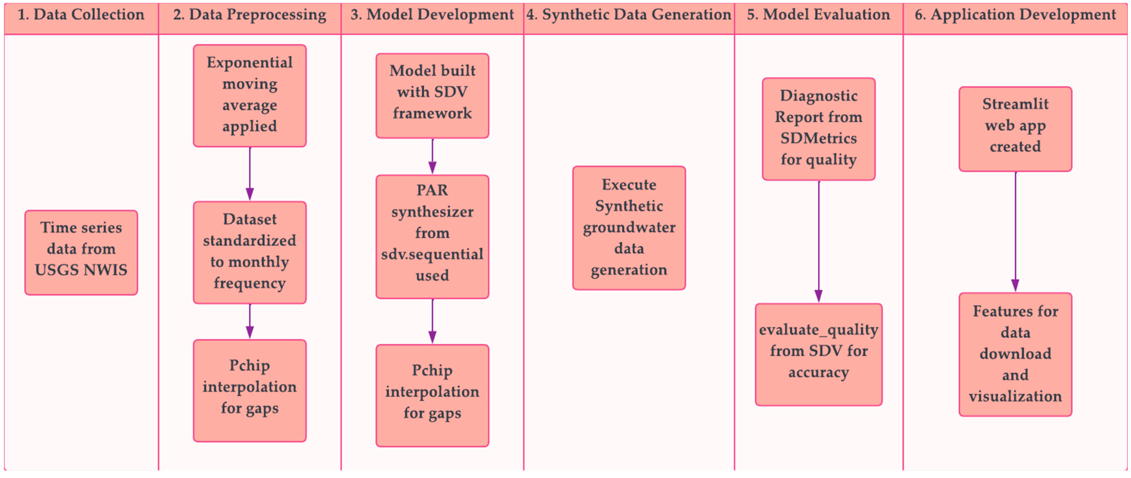
Time series of the groundwater well data for the state of Mississippi were sourced from the United States Geological Survey’s National Water Information System (USGS NWIS), encompassing the period from 1900 to the present. This dataset offers a comprehensive historical perspective on groundwater levels. Wells with fewer than ten observations were excluded to ensure reliability, as such limited data could skew trend analysis.
An exponential moving average with a weighting factor (alpha) of 0.9 was applied to the data for smoothing, chosen to effectively reduce random fluctuations while preserving significant trends.
The dataset was standardized to a monthly frequency, involving the aggregation or interpolation of data points to fit this interval. To fill gaps in the time series, the pchip interpolation method was utilized because of its ability to maintain the inherent characteristics and trends of the data, creating a continuous and realistic dataset for in-depth analysis.
The integrity of the model inputs directly influences the quality of the results, a principle that holds true, especially in the realm of supervised machine learning models where the output is as robust as the input data. In line with this, our approach requires the inputs to be tabular in shape. The data, sourced from USGS NWIS, underwent a rigorous refinement process to meet this requirement. Wells with minimal data records were excluded to ensure a higher level of data integrity (
Table 1). The application of exponential moving averages further refined the data, enhancing its suitability for the machine learning models employed in our ‘Synthetic Wells’ workflow. This dataset, which emphasizes unique well identifiers and smoothed groundwater measurements, is tailored for the specific purpose of meeting our predictive modeling objectives. This approach represents a critical step in our workflow and lays a solid foundation for the innovative methodologies and analyses that follow.
In formulating our approach to simulate groundwater levels across Mississippi, we were met with the challenge of sparse and unevenly distributed data. This situation necessitated a strategy that could make the most of the available information, acknowledging the state’s varied aquifer systems, from the dynamic Mississippi River Valley alluvial aquifer (MRVAA) to the more stable, confined aquifers. Our initial analysis revealed a dataset that was largely representative of the MRVAA. Given this skew, we chose to proceed with a broad dataset for our model’s initial training phase.
This approach was guided by the goal of leveraging the existing data to its fullest extent, recognizing that our model’s output would primarily reflect the characteristics observed in the MRVAA data. This decision was strategic, aimed at laying a groundwork for developing a robust framework capable of handling synthetic data generation. The intent was not to capture every nuance of the aquifer systems but rather to create a versatile dataset that would support the early stages of model development and subsequent refinements.
The development of our method highlights the critical need for specificity and adaptability in groundwater studies, especially when accounting for the distinct hydrogeological features of different aquifers. It is designed to be flexible, allowing researchers to tailor synthetic data generation to the unique attributes of their study areas. This approach not only facilitates methodological refinement but also enhances the relevance and accuracy of models used in groundwater management. By adopting this strategy, we aim to strike a balance between the creation of a comprehensive dataset and the goal of achieving precision in modeling the specific groundwater level fluctuations of various aquifer systems.
2.2. Model
The model for simulating groundwater levels was developed using the Synthetic Data Vault (SDV) framework [
49]. A noteworthy aspect of the SDV is its licensing under the business source license, which is not classified as an open-source license. As per the license, while the SDV is not initially open source, it is likely to become available under an open-source license in the future. Despite this licensing restriction, the SDV was chosen because it is widely recognized and used in the field of data science. Since our study is research oriented, our use of the SDV falls within permissible limits. Its suite of tools and functionalities make it one of the most popular frameworks for handling and generating synthetic time series data.
The SDV is particularly valuable because of its array of helper tools and functions that facilitate the efficient handling and analysis of data. These tools include but are not limited to the SingleTableMetadata class, which is crucial for obtaining a comprehensive understanding and effective structuring of the metadata of the input data. Such capabilities of the SDV framework are pivotal for ensuring that the synthetic time series data that are generated are optimally prepared for further machine learning applications.
The Probabilistic AutoRegressive (PAR) synthesizer model [
50] from the sdv.sequential module was used due to its specialized capabilities in processing sequential, time series data. The PAR model is a neural network-based approach designed to generate new sequences of multidimensional data. Its strength lies in conditioning on consistent, context-specific values, enabling the creation of diverse and realistic data sequences. This feature is particularly beneficial for simulating groundwater levels, as it adeptly handles the multidimensional and temporal nature of the data, aligning closely with the objectives of this study.
In the initial model training, overfitting was a notable issue. Overfitting, a common challenge in machine learning, undermines a model’s ability to perform well on new datasets. This happens when a model excessively learns from the specific details and noise of the training data. To combat this, the training strategy involved limiting the number of epochs. An epoch, a complete pass through the training dataset, influences how well a model learns patterns. While more epochs can improve learning, they also increase the risk of overfitting. In this case, reducing the number of epochs helped the model focus on learning key patterns without absorbing the noise in the data.
In creating the model for groundwater level simulation, the efficiency and utility of the Synthetic Data Vault (SDV) framework were particularly noteworthy. With just a few lines of code, we were able to generate a synthetic time series model. This ease of use underscores the framework’s user-friendly design, enabling the rapid development and deployment of complex models.
Furthermore, the SDV offers an additional module specifically designed for evaluating synthetic data. This module is invaluable for ensuring the quality and accuracy of synthetic time series, providing an essential step in validating the model’s performance. The availability of this evaluation tool within the SDV framework further highlights its comprehensive nature, making it a highly beneficial tool in the realm of data science, particularly for any workflows that require a thorough analysis and validation of synthetic data.
2.3. Web Application
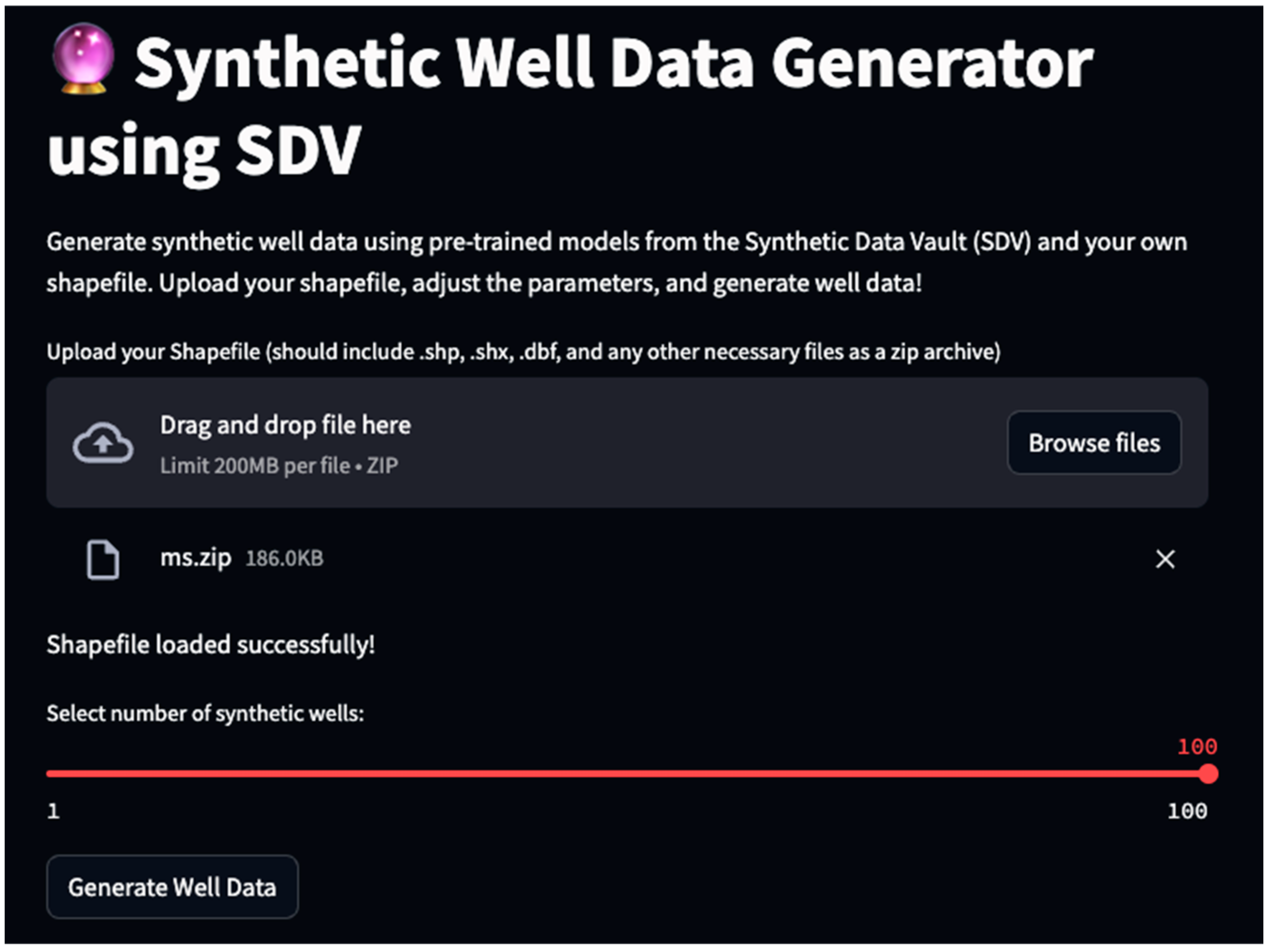
A pivotal component of this research was the creation of a Streamlit-based web application [
48] designed to facilitate the generation and evaluation of synthetic groundwater data. The choice of Streamlit as the platform for this application was driven by its ability to enable the rapid development of user-friendly web apps using Python (v. 3.12). With Streamlit, the entire application was developed in less than 150 lines of code; a feat that would have required more substantial effort and complexity had another framework been used.
Streamlit’s simplicity and efficiency eliminated the need to address the intricacies often associated with web development, such as handling frontend–backend integration, managing multiple frameworks, or delving into JavaScript for interactivity. This approach allowed for a direct focus on the application’s functionality, particularly on leveraging the SDV framework and its PAR model.
Upon initialization, the application loads a pretrained PAR model and sets up necessary metadata using the SingleTableMetadata class, derived from an input CSV file. This ensures the alignment of synthetic data with real-world data structures. Users interact with the application through an intuitive interface, uploading shapefiles to define geographical boundaries for the generation of synthetic well data.
The generate_data function plays a crucial role in creating spatially relevant synthetic data points within a user-defined geographical area. The app allows users to specify the number of synthetic wells, enhancing its flexibility. After generation, the quality of the synthetic dataset is evaluated against real data, ensuring its validity and reliability for representing real-world groundwater dynamics.
For added utility, the application provides options for downloading synthetic data and visualizing specific well time series data. These features, coupled with the app’s ease of use and the efficiency of Streamlit, make this web application a highly effective tool for researchers and practitioners in hydrology. Moreover, combining advanced data science tools with user-centric application design is vital, as this approach offers a comprehensive and accessible solution for analyzing synthetic time series data in groundwater studies.
The current iteration (version 1.0) of the ‘Synthetic Wells’ web application allows users to generate synthetic groundwater datasets tailored to specified geographic regions (
Figure 2 and
Figure 3). However, it is currently limited in its ability to discern and segregate data from multiple aquifers within these regions. To ensure the integrity and specificity of the synthetic datasets, users are encouraged to upload data corresponding to a single aquifer at a time. This practice will help avoid the potential dilution of dataset precision that may occur when data from different aquifers are inadvertently mixed.
Understanding the importance of generating aquifer-specific datasets, there is an ongoing consideration for enhancing the application with a feature that can automatically identify multiple aquifers within the uploaded data. Once identified, the application could then offer users the option to subset the data based on aquifer distinctions. This proposed functionality would significantly refine the application’s ability to produce highly targeted synthetic datasets, thereby enhancing the relevance and applicability of the research outputs.
Implementing such a feature would represent a significant advancement in the application’s capabilities, enabling a more nuanced approach to synthetic dataset generation. It would facilitate a more precise simulation of groundwater levels across diverse hydrological environments, thus supporting the hydrology research community with tools that are not only sophisticated but also highly adaptable to specific research needs.
3. Results
Following the successful compilation of the model, synthetic time series data were generated for approximately 100 wells, each encompassing approximately 35 timesteps. This section presents the findings regarding the model’s performance, focusing on specific metrics and output results derived from the synthetic data. To evaluate the quality and accuracy of the synthesized time series, tools such as evaluate_quality from the Synthetic Data Vault (SDV) and DiagnosticReport from SDMetrics were used. These tools provided insights into the fidelity and statistical properties of synthetic data compared to those of the original datasets. The ensuing analysis offers a critical assessment of the model’s capability to replicate realistic groundwater level dynamics, highlighting the effectiveness of the synthetic data generation process.
3.1. Model Metrics
After generating synthetic time series data for approximately 100 wells, each with approximately 35 timesteps, the performance of the models was evaluated using DiagnosticReport from SDMetrics and evaluate_quality from the SDV. This evaluation focused on the adherence of the synthetic data to the real data’s min/max boundaries and its uniqueness.
The synthetic data adhered to more than 90% of the real data’s min/max boundaries, indicating a high level of fidelity in capturing the range of values. However, more than 10% of the numerical data were missing in the real data, suggesting room for improvement in terms of representing the full variability. A critical observation was that more than 50% of the synthetic rows were identical to the real data, highlighting the need for enhancement of the model’s ability to generate unique data points.
The overall quality score was calculated to be 70.94%. The average of the column shape score and the column pair trend score was 53.97%, indicating only moderate similarity in distribution shapes between the synthetic and real data. The score for column pair trends was more promising at 87.91%, reflecting a strong alignment in trends and relationships between column pairs.
The results occasionally varied, sometimes yielding data with no danger warnings, suggesting a degree of randomness in the model’s output. This variability indicates that, while the model can achieve high-quality outputs, consistency remains an area for improvement.
Future enhancements to the model could involve increasing the size and diversity of the training dataset to enrich the learning process. Additionally, fine-tuning the model parameters and exploring advanced neural network architectures may further improve the model’s ability to generate more diverse and realistic synthetic data. These improvements aim to reduce the occurrence of direct data replication, thereby increasing the overall quality and utility of the synthetic dataset for comprehensive hydrological analysis.
3.2. Effective Use of the Web Application in Data Synthesis
The Streamlit web application was instrumental in this research, particularly because of its ability to generate synthetic groundwater data tailored to user-defined parameters. A standout feature of the application is its flexibility in allowing users to specify the number of wells and select their geographic region of interest. This adaptability ensures that the generated datasets are region specific and can also vary in size based on the user’s needs.
Users have the advantage of inputting their geographic data into the app, leading to the creation of synthetic time series data that align closely with the chosen areas. This level of customization in data generation represents a significant advancement in creating relevant and practical synthetic datasets.
In addition to data generation, the integration of quality assessment tools from the SDV played a crucial role in the prompt validation of synthetic data. This feature provided immediate and actionable feedback, enhancing the trustworthiness and precision of the datasets created. Additionally, the app’s data visualization functionalities allowed for an in-depth exploration of groundwater level trends and patterns in selected wells.
This web application stands as an asset not only for this study but also for the hydrology research community at large. This study highlights the seamless application of sophisticated data science techniques in hydrological research, offering a user-friendly platform for the generation and analysis of customized synthetic data. The tool can be found at the following URL:
https://github.com/igwm/synthetic_wells (accessed on 20 March 2024) [
51].
3.3. Case Study: Enhancing Groundwater Level Forecasts Using Synthetic Data
While the previous sections of this research have emphasized the generation and initial evaluation of synthetic groundwater level data, the following section aims to demonstrate the effectiveness of synthetic data in improving the accuracy of time series forecasting models. Given the challenges of obtaining sparse and irregular real-world data, the integration of synthetic data is a promising solution.
3.3.1. Methodology
The case study employed two datasets: historical groundwater measurements of 1306 wells across the State of Mississippi and synthetic groundwater level data for 100 wells across the MRVAA. The synthetic dataset was generated using the SDV as described in the methods section, thus ensuring realistic and contextually relevant data. To assess the impact of synthetic data, we focused on the time series forecasting model ARIMA.
The ARIMA model was selected due to its established effectiveness in time series analysis, especially in hydrological studies. Its ability to model the temporal dynamics, trends and seasonality of groundwater levels aligns well with this study’s goals. ARIMA’s broad acceptance in hydrology offers a solid foundation for quantifying the improvements synthetic data bring to forecasting accuracy, highlighting the benefits of integrating advanced machine learning techniques in water resource management [
52,
53].
The analysis was conducted in two primary stages:
Data preparation: This stage involved merging the historical and synthetic datasets, with a focus on key columns essential for time series analysis, namely, GW_measurement and Date. To align the data across different wells, the data were aggregated monthly, creating a standardized and uniform temporal framework for subsequent analysis. When a well had multiple measurements in a month, the mean of these values was calculated to standardize the dataset to a monthly frequency. This ensured each well was consistently represented by a single, average measurement per month.
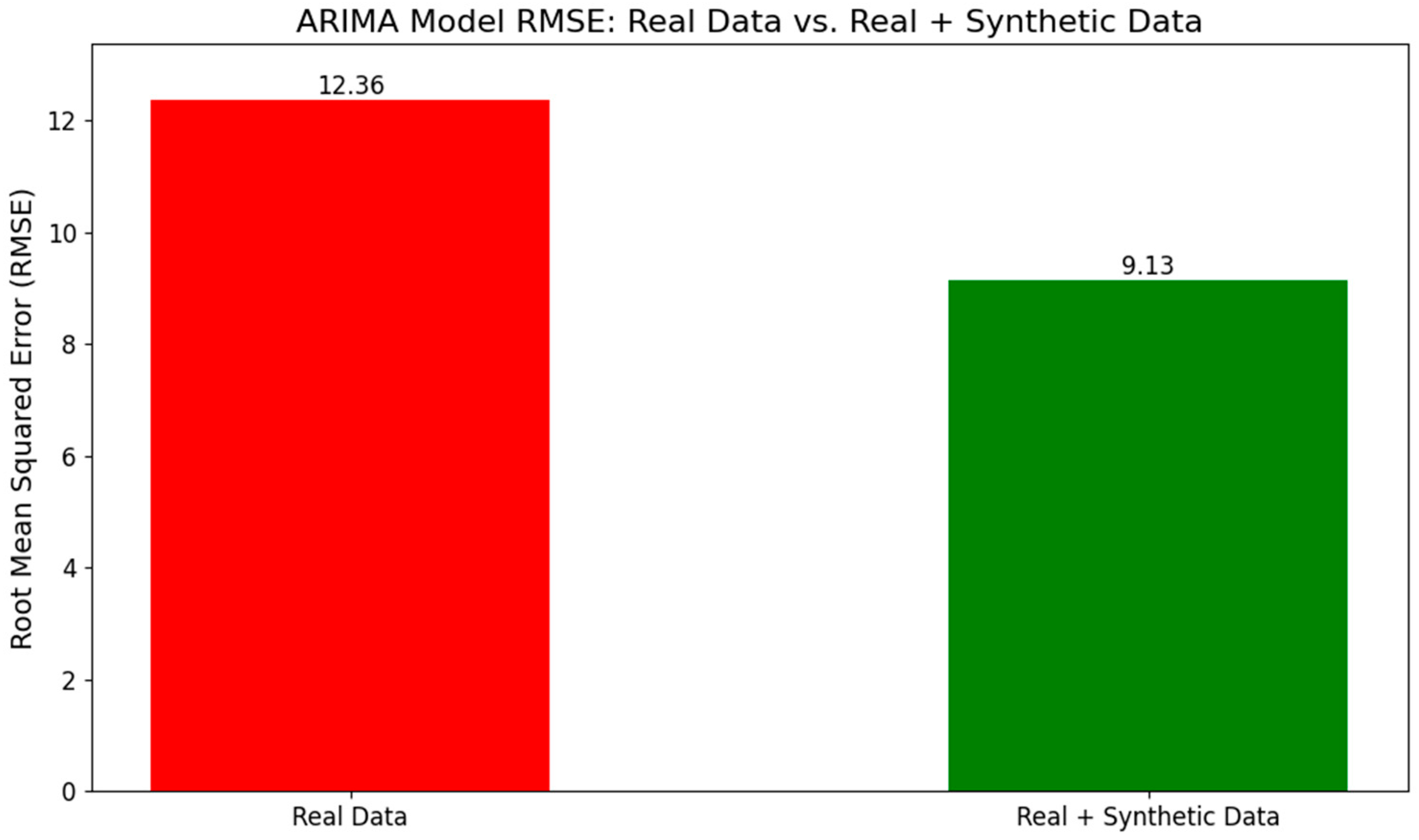
Model training and evaluation: In this stage, two separate ARIMA models were developed and assessed. The first model utilized the merged dataset comprising both real and synthetic data, while the second model was trained exclusively on real data. These models were evaluated based on their root mean squared error (RMSE) performance, which provides a quantitative measure of forecasting accuracy.
3.3.2. Results
Incorporating a combination of real and synthetic data into the ARIMA model yielded a significant improvement in model performance, as evidenced by the marked reduction in the root mean squared error (RMSE) from approximately 12.36 ft when relying solely on real data to approximately 9.13 ft (
Figure 4). This result underscores the potential of synthetic data to enhance the precision of time series forecasting models, a particularly valuable advantage in regions with limited data availability. The synthetic data effectively serve as a bridge, bolstering the overall reliability of the dataset.
Including synthetic data has broadened the model’s capacity to detect and analyze a diverse array of temporal patterns, thereby elevating its predictive accuracy in groundwater management. This improvement in analytical capabilities holds significant promise, especially in regions where data scarcity has historically hindered robust decision-making processes. Furthermore, this advancement not only refines strategies for groundwater conservation and utilization but also marks the beginning of an innovative approach to advance predictive analytics in the field.
4. Discussion
The integration of synthetic time series data into machine learning workflows for groundwater modeling, as presented in this study, represents a significant advance in the utilization of data science techniques within the realm of hydrology. This discussion aims to contextualize our findings within the broader scope of existing methods, highlight the challenges encountered, and outline potential future research directions.
Our approach to generating synthetic time series data represents a response to the pervasive challenge of data scarcity in groundwater studies. The success of this methodology in simulating realistic groundwater level variations demonstrates its potential as a valuable tool in hydrological modeling. This study extends the application of synthetic data, which are traditionally used in fields such as finance and healthcare, to address specific challenges in groundwater management, thereby enriching the dataset and enhancing model accuracy in scenarios where real data are limited or nonexistent.
One of the primary limitations of this study is its focus on existing time series data, without incorporating additional environmental variables such as precipitation, temperature, and land use changes. This approach, while foundational, limits the model’s ability to fully encapsulate the complex interactions affecting groundwater levels.
Furthermore, the generalizability of the findings may be constrained by the specific characteristics of the dataset employed. The dynamics of groundwater can vary widely across different geographical areas and aquifer systems, influenced by diverse geological formations and hydrological cycles. This study’s model, primarily trained on data from Mississippi, USA, may not capture these variations accurately when applied to other regions without further adaptation.
Another critical limitation is this study’s temporal resolution and coverage. The dataset’s span and granularity might not adequately represent long-term groundwater trends or the intricacies of seasonal variations, especially in areas subject to significant climatic variability. This limitation could potentially impact the model’s predictive accuracy for future groundwater levels under scenarios of changing climate conditions.
The development and application of the ‘Synthetic Wells’ workflow highlights the need for methodological refinement in the generation of synthetic data. Achieving a balance between replicating the fidelity of real-world data and ensuring the diversity of synthetic outputs was a key challenge. Future efforts should focus on enhancing the algorithms to more accurately capture the intricate patterns of groundwater level variability while also generating data points that are distinct yet representative of real-world scenarios.
The potential applications of this approach are not confined to groundwater modeling alone. The method can be adapted to other environmental and geospatial studies where data limitations are prevalent. Looking forward, exploring the use of synthetic time series data in conjunction with other types of environmental data, such as satellite imagery or sensor readings, could provide a more comprehensive understanding of various natural processes. Future research should focus on enhancing the dataset with additional environmental variables to capture the multifaceted influences on groundwater levels more comprehensively. There is also a critical need to test and refine the model across different geographical areas and aquifer systems to improve its generalizability. Expanding the dataset to include longer time series with higher resolution, alongside incorporating future climate scenarios, will significantly enhance the model’s predictive accuracy. These steps will ensure that the synthetic data generated are more robust and applicable for advanced groundwater management and planning efforts in the face of climate change.
The practical implications of employing synthetic time series data in groundwater studies include enhanced decision-making and policy formulation in water resource management. By providing a more robust and comprehensive dataset, this approach supports the development of more accurate models, which are crucial for effective water resource planning and management, especially in the face of climate change and increasing water demand. The integration of advanced data synthesis techniques in hydrological models holds promise for informing policy decisions and ensuring sustainable water resource management.
This study highlights the significant potential of incorporating synthetic time series data to profoundly enhance algorithms and model development in groundwater modeling. Tackling the prevalent issue of data scarcity in hydrology, this method markedly improves the predictive accuracy of groundwater level models, representing a key innovation in the field. This approach expands the scope of analytical tools available for groundwater research and aids in driving more data-informed decisions in water resource management and policy. This study sets the groundwork for future exploration, signaling further progress in applying machine learning techniques in environmental studies. This advancement is pivotal for deepening our understanding and effective management of water resources, leading to more efficient and sustainable methods.
Author Contributions
Conceptualization, H.Y. and S.T.P.; methodology, S.T.P.; software, S.T.P.; validation, S.T.P. and L.D.Y.; formal analysis, S.T.P.; data curation, S.T.P.; writing—original draft preparation, S.T.P.; writing—review and editing, H.Y. and L.D.Y.; project administration, H.Y. and L.D.Y.; funding acquisition, H.Y. All authors have read and agreed to the published version of the manuscript.
Funding
This work was funded by a research grant awarded by the National Science Foundation (Award No.: OIA 2019561).
Data Availability Statement
Data are contained within the article.
Conflicts of Interest
The authors declare no conflicts of interest. The funders had no role in the design of the study; in the collection, analyses, or interpretation of data; in the writing of the manuscript; or in the decision to publish the results.
References
- Famiglietti, J.S. The Global Groundwater Crisis. Nat. Clim. Chang. 2014, 4, 945–948. [Google Scholar] [CrossRef]
- McDonough, L.K.; Santos, I.R.; Andersen, M.S.; O’Carroll, D.M.; Rutlidge, H.; Meredith, K.; Oudone, P.; Bridgeman, J.; Gooddy, D.C.; Sorensen, J.P.R.; et al. Changes in Global Groundwater Organic Carbon Driven by Climate Change and Urbanization. Nat. Commun. 2020, 11, 1279. [Google Scholar] [CrossRef] [PubMed]
- Misra, A.K. Impact of Urbanization on the Hydrology of Ganga Basin (India). Water Resour. Manag. 2011, 25, 705–719. [Google Scholar] [CrossRef]
- Tao, H.; Hameed, M.M.; Marhoon, H.A.; Zounemat-Kermani, M.; Heddam, S.; Kim, S.; Sulaiman, S.O.; Tan, M.L.; Sa’adi, Z.; Mehr, A.D.; et al. Groundwater Level Prediction Using Machine Learning Models: A Comprehensive Review. Neurocomputing 2022, 489, 271–308. [Google Scholar] [CrossRef]
- Sun, A.Y. Predicting Groundwater Level Changes Using GRACE Data. Water Resour. Res. 2013, 49, 5900–5912. [Google Scholar] [CrossRef]
- Ahmadi, A.; Olyaei, M.; Heydari, Z.; Emami, M.; Zeynolabedin, A.; Ghomlaghi, A.; Daccache, A.; Fogg, G.E.; Sadegh, M. Groundwater Level Modeling with Machine Learning: A Systematic Review and Meta-Analysis. Water 2022, 14, 949. [Google Scholar] [CrossRef]
- Fabio, D.N.; Abba, S.I.; Pham, B.Q.; Islam, A.R.M.T.; Talukdar, S.; Francesco, G. Groundwater Level Forecasting in Northern Bangladesh Using Nonlinear Autoregressive Exogenous (NARX) and Extreme Learning Machine (ELM) Neural Networks. Arab. J. Geosci. 2022, 15, 647. [Google Scholar] [CrossRef]
- Jasechko, S.; Seybold, H.; Perrone, D.; Fan, Y.; Shamsudduha, M.; Taylor, R.G.; Fallatah, O.; Kirchner, J.W. Rapid Groundwater Decline and Some Cases of Recovery in Aquifers Globally. Nature 2024, 625, 715–721. [Google Scholar] [CrossRef] [PubMed]
- Jordon, J.; Szpruch, L.; Houssiau, F.; Bottarelli, M.; Cherubin, G.; Maple, C.; Cohen, S.N.; Weller, A. Synthetic Data—What, Why and How? arXiv 2022, arXiv:2205.03257. [Google Scholar]
- Rizzato, M.; Wallart, J.; Geissler, C.; Morizet, N.; Boumlaik, N. Generative Adversarial Networks Applied to Synthetic Financial Scenarios Generation. Soc. Sci. Res. Netw. 2022, 623, 128899. [Google Scholar] [CrossRef]
- Borgomeo, E.; Farmer, C.L.; Hall, J.W. Numerical Rivers: A Synthetic Streamflow Generator for Water Resources Vulnerability Assessments. Water Resour. Res. 2015, 51, 5382–5405. [Google Scholar] [CrossRef]
- Benoit, L.; Mariethoz, G. Generating Synthetic Rainfall with Geostatistical Simulations. WIREs Water 2017, 4, e1199. [Google Scholar] [CrossRef]
- McAfee, S.A.; Pederson, G.T.; Woodhouse, C.A.; McCabe, G.J. Application of Synthetic Scenarios to Address Water Resource Concerns: A Management-Guided Case Study from the Upper Colorado River Basin. Clim. Serv. 2017, 8, 26–35. [Google Scholar] [CrossRef]
- Kilsby, C.G.; Jones, P.D.; Burton, A.; Ford, A.C.; Fowler, H.J.; Harpham, C.; James, P.; Smith, A.; Wilby, R.L. A Daily Weather Generator for Use in Climate Change Studies. Environ. Model. Softw. 2007, 22, 1705–1719. [Google Scholar] [CrossRef]
- Zhang, C.; Kuppannagari, S.R.; Kannan, R.; Prasanna, V.K. Generative Adversarial Network for Synthetic Time Series Data Generation in Smart Grids. In Proceedings of the 2018 IEEE International Conference on Communications, Control, and Computing Technologies for Smart Grids (SmartGridComm), Aalborg, Denmark, 29–31 October 2018; pp. 1–6. [Google Scholar]
- Zheng, X.; Xu, N.; Trinh, L.; Wu, D.; Huang, T.; Sivaranjani, S.; Liu, Y.; Xie, L. A Multi-Scale Time-Series Dataset with Benchmark for Machine Learning in Decarbonized Energy Grids. Sci. Data 2022, 9, 359. [Google Scholar] [CrossRef] [PubMed]
- Chen, R.J.; Lu, M.Y.; Chen, T.Y.; Williamson, D.F.K.; Mahmood, F. Synthetic Data in Machine Learning for Medicine and Healthcare. Nat. Biomed. Eng. 2021, 5, 493–497. [Google Scholar] [CrossRef] [PubMed]
- Dahmen, J.; Cook, D. SynSys: A Synthetic Data Generation System for Healthcare Applications. Sensors 2019, 19, 1181. [Google Scholar] [CrossRef] [PubMed]
- Menichini, M.; Franceschi, L.; Raco, B.; Masetti, G.; Scozzari, A.; Doveri, M. Groundwater Modeling with Process-Based and Data-Driven Approaches in the Context of Climate Change. Water 2022, 14, 3956. [Google Scholar] [CrossRef]
- Goodfellow, I.J.; Pouget-Abadie, J.; Mirza, M.; Xu, B.; Warde-Farley, D.; Ozair, S.; Courville, A.; Bengio, Y. Generative Adversarial Networks. arXiv, arXiv:1406.2661.
- Karras, T.; Laine, S.; Aila, T. A Style-Based Generator Architecture for Generative Adversarial Networks. In Proceedings of the 2019 IEEE/CVF Conference on Computer Vision and Pattern Recognition (CVPR), Long Beach, CA, USA, 15–20 June 2019. [Google Scholar] [CrossRef]
- Pan, Z.; Yu, W.; Yi, X.; Khan, A.; Yuan, F.; Zheng, Y. Recent Progress on Generative Adversarial Networks (GANs): A Survey. IEEE Access 2019, 7, 36322–36333. [Google Scholar] [CrossRef]
- Gong, X.; Chang, S.; Jiang, Y.; Wang, Z. AutoGAN: Neural Architecture Search for Generative Adversarial Networks. In Proceedings of the 2019 IEEE/CVF International Conference on Computer Vision (ICCV), Seoul, Republic of Korea, 27 October–2 November 2019. [Google Scholar] [CrossRef]
- Lee, S.; Kim, J.; Lee, G.; Hong, J.; Bae, J.H.; Lim, K.J. Prediction of Aquatic Ecosystem Health Indices through Machine Learning Models Using the WGAN-Based Data Augmentation Method. Sustainability 2021, 13, 10435. [Google Scholar] [CrossRef]
- Oyelade, O.N.; Ezugwu, A.E.; Almutairi, M.S.; Saha, A.K.; Abualigah, L.; Chiroma, H. A Generative Adversarial Network for Synthetization of Regions of Interest Based on Digital Mammograms. Sci. Rep. 2022, 12, 6166. [Google Scholar] [CrossRef] [PubMed]
- Saxena, D.; Cao, J. Generative Adversarial Networks (GANs). ACM Comput. Surv. 2021, 54, 1–42. [Google Scholar] [CrossRef]
- Jaeger, H. The “Echo State” Approach to Analysing and Training Recurrent Neural Networks—With an Erratum Note; GMD Technical Report 148; German National Research Center for Information Technology: Bonn, Germany, 2001; p. 13. [Google Scholar]
- Sacchi, R.; Ozturk, M.C.; Principe, J.C.; Carneiro, A.A.F.M.; da Silva, I.N. Water Inflow Forecasting Using the Echo State Network: A Brazilian Case Study. In Proceedings of the 2007 International Joint Conference on Neural Networks, Orlando, FL, USA, 12–17 August 2007; pp. 2403–2408. [Google Scholar]
- Hung, M.D.; Dung, N.T. Application of Echo State Network for the Forecast of Air Quality. Vietnam J. Sci. Technol. 2016, 54, 54–63. [Google Scholar] [CrossRef]
- de Aquino, R.R.B.; Neto, O.N.; Souza, R.B.; Lira, M.M.S.; Carvalho, M.A.; Ludermir, T.B.; Ferreira, A.A. Investigating the Use of Echo State Networks for Prediction of Wind Power Generation. In Proceedings of the 2014 IEEE Symposium on Computational Intelligence for Engineering Solutions (CIES), Orlando, FL, USA, 9–12 December 2014; pp. 148–154. [Google Scholar]
- De Vos, N.J. Echo State Networks as an Alternative to Traditional Artificial Neural Networks in Rainfall–Runoff Modelling. Hydrol. Earth Syst. Sci. 2013, 17, 253–267. [Google Scholar] [CrossRef]
- Deihimi, A.; Showkati, H. Application of Echo State Networks in Short-Term Electric Load Forecasting. Energy 2012, 39, 327–340. [Google Scholar] [CrossRef]
- Ribeiro, G.T.; Sauer, J.G.; Fraccanabbia, N.; Mariani, V.C.; Coelho, L.d.S. Bayesian Optimized Echo State Network Applied to Short-Term Load Forecasting. Energies 2020, 13, 2390. [Google Scholar] [CrossRef]
- Dan, J.; Guo, W.; Shi, W.; Fang, B.; Zhang, T. Deterministic Echo State Networks Based Stock Price Forecasting. Abstr. Appl. Anal. 2014, 2014, 137148. [Google Scholar] [CrossRef]
- Kingma, D.P.; Welling, M. Auto-Encoding Variational Bayes. arXiv 2022, arXiv:1312.6114. [Google Scholar]
- Koneripalli, K.; Lohit, S.; Anirudh, R.; Turaga, P. Rate-Invariant Autoencoding of Time-Series. In Proceedings of the ICASSP 2020—2020 IEEE International Conference on Acoustics, Speech and Signal Processing (ICASSP), Barcelona, Spain, 4–8 May 2020; pp. 3732–3736. [Google Scholar] [CrossRef]
- Kavran, D.; Žalik, B.; Lukač, N. Time Series Augmentation Based on Beta-VAE to Improve Classification Performance. In Proceedings of the 14th International Conferenceon Agents and Artificial Intelligence (ICAART 2022), Online, 3–5 February 2022; pp. 15–23. [Google Scholar]
- Ma, X.; Raginsky, M.; Cangellaris, A.C. A Machine Learning Methodology for Inferring Network S-Parameters in the Presence of Variability. In Proceedings of the 2018 IEEE 22nd Workshop on Signal and Power Integrity (SPI), Brest, France, 22–25 May 2018; pp. 1–4. [Google Scholar]
- Goubeaud, M.; Joußen, P.; Gmyrek, N.; Ghorban, F.; Schelkes, L.; Kummert, A. Using Variational Autoencoder to Augment Sparse Time Series Datasets. In Proceedings of the 2021 7th International Conference on Optimization and Applications (ICOA), Wolfenbüttel, Germany, 19–20 May 2021; pp. 1–6. [Google Scholar]
- Yokkampon, U.; Mowshowitz, A.; Chumkamon, S.; Hayashi, E. Robust Unsupervised Anomaly Detection With Variational Autoencoder in Multivariate Time Series Data. IEEE Access 2022, 10, 57835–57849. [Google Scholar] [CrossRef]
- Interpretation for Variational Autoencoder Used to Generate Financial Synthetic Tabular Data. Available online: https://www.mdpi.com/1999-4893/16/2/121 (accessed on 19 January 2024).
- Shao, H.; Yao, S.; Sun, D.; Zhang, A.; Liu, S.; Liu, D.; Wang, J.; Abdelzaher, T. Controllable Variational Autoencoder. arXiv 2020, arXiv:2004.05988v5. [Google Scholar]
- Rasmussen, C.E.; Williams, C.K.I. Gaussian Processes for Machine Learning; The MIT Press: Cambridge, MA, USA, 2005; ISBN 978-0-262-18253-9. [Google Scholar]
- Zhang, S.; Bai, Y.; He, X.; Jiang, Z.; Li, T.; Gong, F.; Yu, S.; Pan, D. Spatial and Temporal Variations in Sea Surface pCO2 and Air-Sea Flux of CO2 in the Bering Sea Revealed by Satellite-Based Data during 2003–2019. Front. Mar. Sci. 2023, 10, 1099916. [Google Scholar] [CrossRef]
- Paton, F.; McNicholas, P.D. Detecting British Columbia Coastal Rainfall Patterns by Clustering Gaussian Processes. Environmetrics 2020, 31, e2631. [Google Scholar] [CrossRef]
- Berns, F.; Hüwel, J.; Beecks, C. Automated Model Inference for Gaussian Processes: An Overview of State-of-the-Art Methods and Algorithms. SN Comput. Sci. 2022, 3, 300. [Google Scholar] [CrossRef] [PubMed]
- Wu, F.; Stevens, N.; Strycker, L.D.; Rottenberg, F. Comparative Study of Gaussian Processes, Multi Layer Perceptrons, and Deep Kernel Learning for Indoor Visible Light Positioning Systems. In Proceedings of the 2023 13th International Conference on Indoor Positioning and Indoor Navigation (IPIN), Nuremberg, Germany, 25–28 September 2023; pp. 1–6. [Google Scholar]
- Streamlit Docs. Available online: https://docs.streamlit.io/ (accessed on 19 January 2024).
- Patki, N.; Wedge, R.; Veeramachaneni, K. The Synthetic Data Vault. In Proceedings of the 2016 IEEE International Conference on Data Science and Advanced Analytics (DSAA), Montreal, QC, Canada, 17–19 October 2016; pp. 399–410. [Google Scholar]
- Zhang, K.; Patki, N.; Veeramachaneni, K. Sequential Models in the Synthetic Data Vault. arXiv 2022, arXiv:2207.14406. [Google Scholar]
- Integrated Groundwater Management Project. Code. Available online: https://github.com/igwm/synthetic_wells (accessed on 20 March 2024).
- Harvey, A.C.; Pierse, R.G. Estimating Missing Observations in Economic Time Series. J. Am. Stat. Assoc. 1984, 79, 125–131. [Google Scholar] [CrossRef]
- Kaur, J.; Parmar, K.S.; Singh, S. Autoregressive Models in Environmental Forecasting Time Series: A Theoretical and Application Review. Environ. Sci. Pollut. Res. 2023, 30, 19617–19641. [Google Scholar] [CrossRef]
| Disclaimer/Publisher’s Note: The statements, opinions and data contained in all publications are solely those of the individual author(s) and contributor(s) and not of MDPI and/or the editor(s). MDPI and/or the editor(s) disclaim responsibility for any injury to people or property resulting from any ideas, methods, instructions or products referred to in the content. |
© 2024 by the authors. Licensee MDPI, Basel, Switzerland. This article is an open access article distributed under the terms and conditions of the Creative Commons Attribution (CC BY) license (https://creativecommons.org/licenses/by/4.0/).


