Interpretation for Variational Autoencoder Used to Generate Financial Synthetic Tabular Data

Abstract

Synthetic data, artificially generated by computer programs, has become more widely used in the financial domain to mitigate privacy concerns. Variational Autoencoder (VAE) is one of the most popular deep-learning models for generating synthetic data. However, VAE is often considered a “black box” due to its opaqueness. Although some studies have been conducted to provide explanatory insights into VAE, research focusing on explaining how the input data could influence VAE to create synthetic data, especially for tabular data, is still lacking. However, in the financial industry, most data are stored in a tabular format. This paper proposes a sensitivity-based method to assess the impact of inputted tabular data on how VAE synthesizes data. This sensitivity-based method can provide both global and local interpretations efficiently and intuitively. To test this method, a simulated dataset and three Kaggle banking tabular datasets were employed. The results confirmed the applicability of this proposed method.

1. Introduction

The past decades have witnessed the production of new data faster than ever in history [1]. In the banking industry, a large amount of complex data, including continuous and categorical data, is generated daily, and stored in a tabular format [2]. Banks could use their stored tabular data to extract actionable business insights to improve their products and services. However, real data usage is sometimes limited because of customer privacy concerns. Due to the high sensitivity of financial data and the restrictions of regulatory norms, the banking industry is a representative field where, in many scenarios, real data is not accessible for analysis [2].

One possible solution to resolve the concerns of violating customers’ privacy is to replace real data with synthetic data, which is artificially generated by computer programs rather than being created by real-world events. Creating synthetic data that captures as many of the complexities of the original data as possible, such as dependencies and distributions in real data, could also bring many other benefits [3]. The advantages of synthetic data in the banking industry include, but are not limited to, the ability to overcome real data usage limitations, to provide more training data for machine learning (ML) models to improve performance and reduce bias, and to simulate future scenarios through data augmentation [4].

There exist many approaches for synthetic tabular data generation. A straightforward approach is to use statistical techniques, such as masking, which replaces parts of a dataset with random information; coarsening, which reduces the precision of some data in a dataset; and mimicking, which adds randomness to a dataset [4]. However, one significant disadvantage of these statistical techniques is that the relationship between different columns cannot be well preserved. Hence, the method of sampling new data from joint distributions learned from an original dataset was proposed [5]. Although joint distributions can capture some potential connections between columns in a tabular dataset, the difficulty of learning all the joint distributions and relationships of a tabular dataset would increase as the complexity of the dataset increases. Even though statistical approaches, playing dominant roles in synthetic data generation for a long time in the past, are fast and easy to implement, a more robust model to tackle the complexity of data is especially needed for the banking industry, where the datasets are usually complex. Recent advancements in deep learning have made generative algorithms more popular for data synthesis [5]. Variational Autoencoders (VAEs) and Generative Adversarial Networks (GANs) are two deep-learning models that are commonly used for synthetic data generation [6]. Although GANs have been proven to generate more realistic images compared with VAEs in synthetic image data generation, the same cannot be assumed for synthetic tabular data generation in financial applications [7]. A study compares the performance of VAEs and GANs in generating synthetic tabular data, showing that while GANs outperform VAEs in synthesizing mostly categorical data types, VAEs perform better in synthesizing continuous data types and datasets with a mix of continuous and categorical data [8]. As financial datasets are often mixed datasets containing continuous data and categorical variables, this paper focuses on studying VAEs for synthetic tabular data generation.

Despite their superior performance, deep-learning models such as the VAE are usually labelled as “black boxes” due to their opaqueness [9]. Data scientists cannot explain the reasons behind the decisions made by the deep-learning models to the fullest extent. However, in reality, the interpretability of deep-learning models is crucial for the scientists who invent the model, the software developers who implement the model, and the clients influenced by the model. This calls for building trust toward the deep-learning models [10]. In VAEs, understanding the decision-making process or the synthetic data generation process is inextricably linked to the latent representation/space of a VAE since synthetic data is produced by using the latent representation that captures the critical information of input data [11]. Being able to understand the relationship between input features in an original dataset and the resulting latent representation in a VAE can enhance the reliability and trustworthiness of synthetic data. More importantly, by identifying which parts of the real dataset are most influential in the latent space, one can improve computational efficiency by removing unnecessary features when generating synthetic tabular data, particularly in the case of banking data that contains many features. Thus, this paper aims to study the impact of each input feature in an original financial tabular dataset on the latent representation of a VAE used to generate synthetic data.

Although little research has been conducted to investigate how each input feature in a tabular dataset could affect the latent space of a VAE, a similar research topic discussing approaches to explain how input variables influence outputs in a Multilayer Perceptron (MLP) can be found in papers related to sensitivity analysis [12]. As the encoder of a VAE can be treated as an MLP, we could leverage the idea of sensitivity to interpret the latent space in VAE. The contributions of this paper can be summarized as follows:

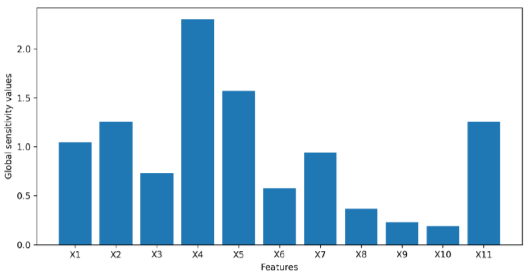
• We extend the idea of first-order sensitivity to a generative model, VAE, to assess the input feature importance when a VAE is used to generate financial synthetic tabular data. As experimental results in this paper show, measuring feature importance by sensitivity can provide both global and local explanations for how a VAE synthesizes tabular data intuitively and efficiently.
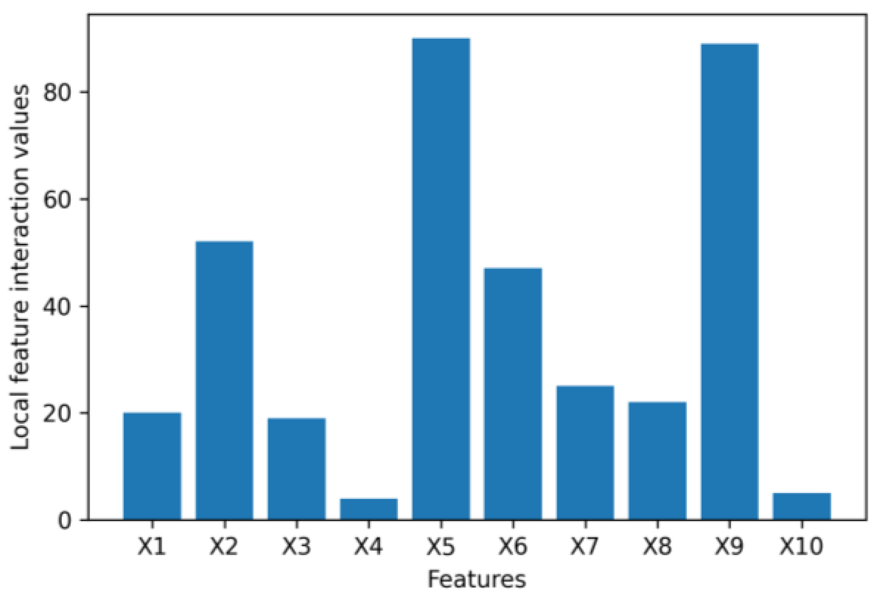
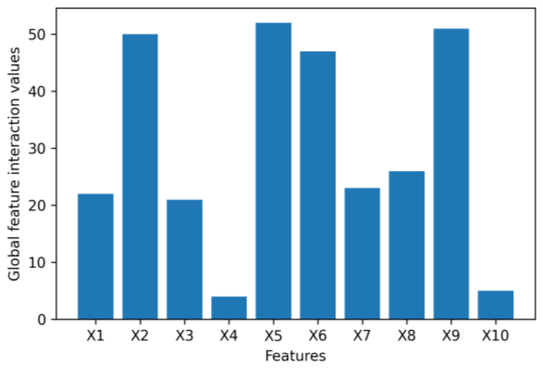
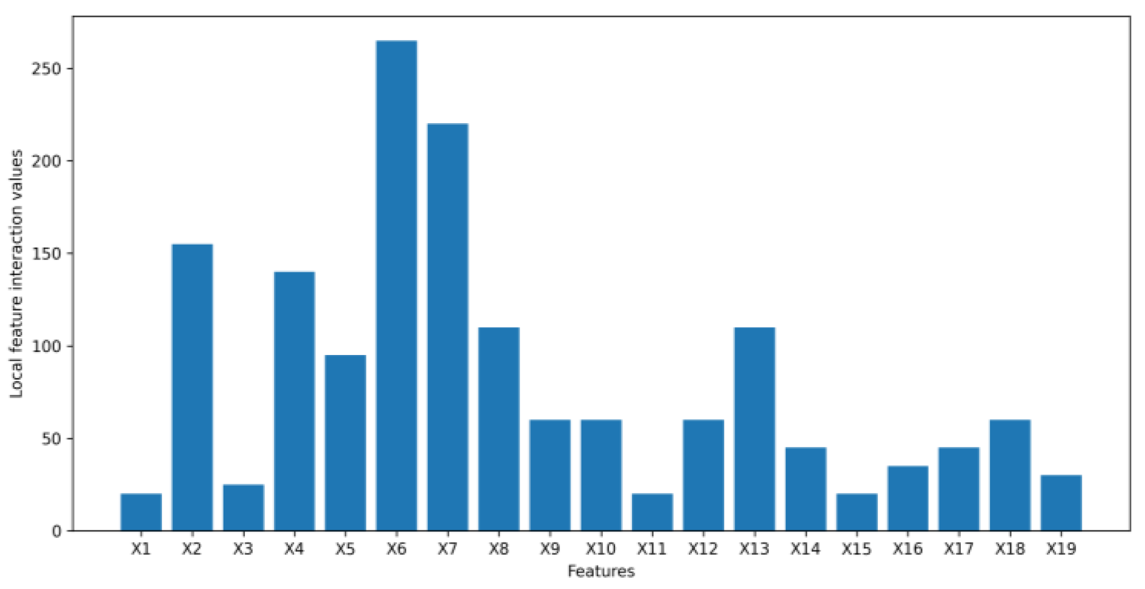
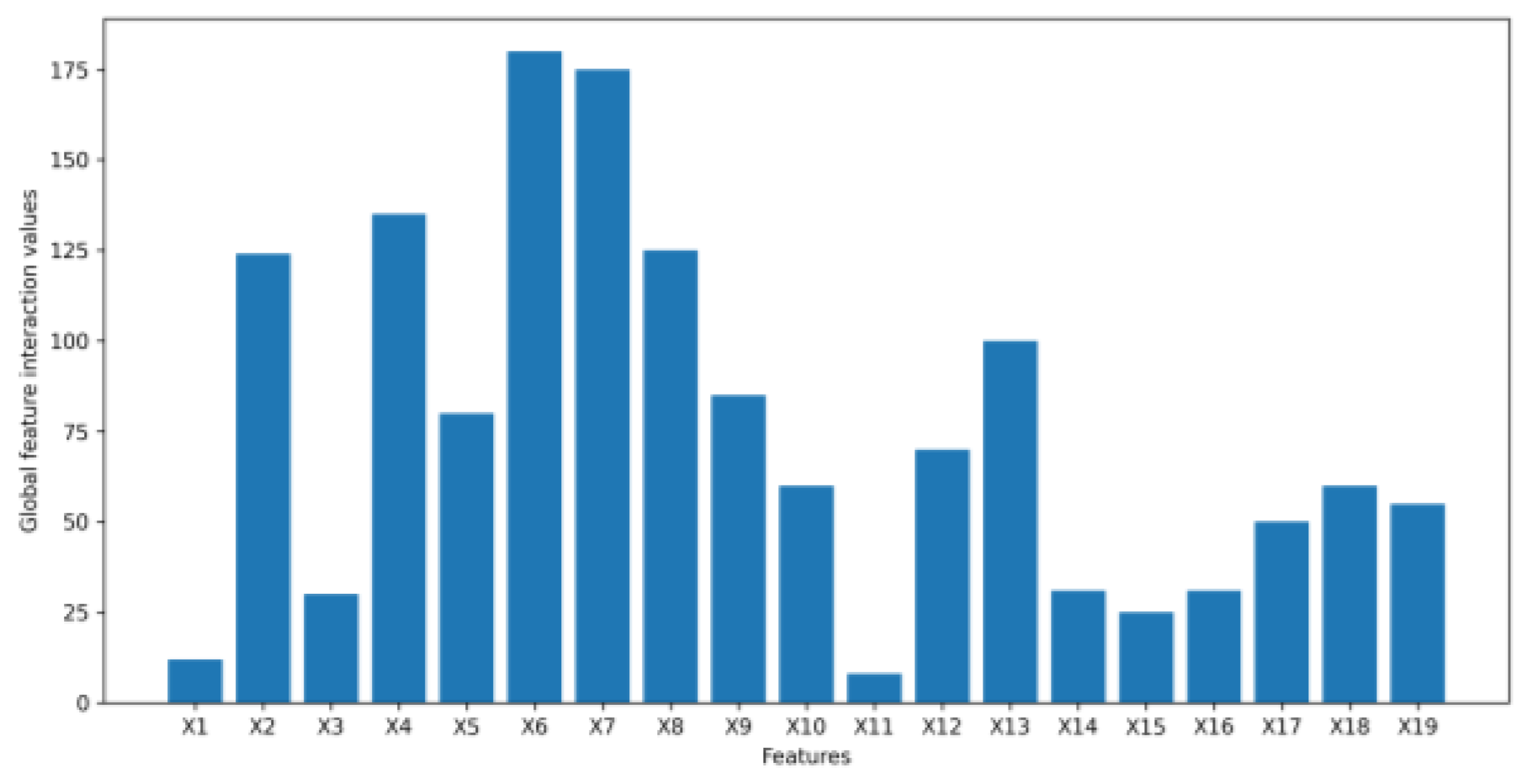
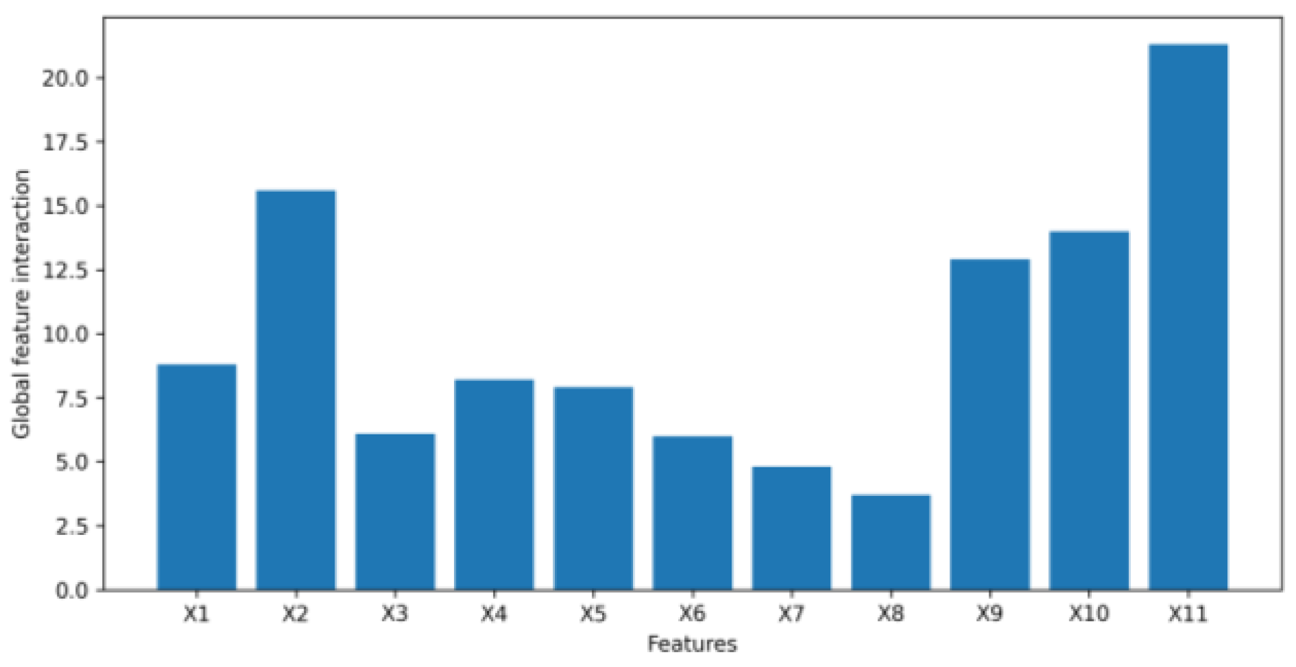
• We leverage the idea of a second-order partial derivative test to investigate feature interactions in an original tabular dataset that goes into a VAE to synthesize data. Measuring the feature interactions of a feature with the rest of the features can help us determine if we can safely remove the feature from a tabular dataset to reduce the dimensionality of the dataset to speed up the process of generating synthetic data without affecting the quality of the synthetic data being generated.

The remaining part of this paper is organized as follows: Section 2 reviews state-of-the-art methods that could provide explanatory insights into VAE data synthesis and the literature, which inspired the authors to design the methodology. Section 3 describes a detailed methodology and four experiments to test the method. Section 4 demonstrates the results obtained using the method described in Section 3. Section 5 discusses the results and future improvements which can be made to this research topic. Section 6 concludes and summarizes this paper.

2. Literature Review

This section reviews existing methodologies, including TabNet, PCA, VEGA, and SOM-VAE, that can interpret the impact of individual input features in a dataset on how VAE generates synthetic data and sensitivity analysis of MLP, which can be utilized to investigate how each input feature in a tabular dataset influences the latent space.

Recently, various TabNet-based deep learning architectures have been developed to effectively identify salient features of a dataset for a given task, enabling interpretability [13]. TabNet, an interpretable ML model created by Google AI, is designed to efficiently handle large amounts of tabular data by using an attention mechanism to select important features for a specific task [14]. While the attention mechanism in TabNet allows for automatic feature selection, interpreting the mechanism and understanding why certain features are considered more important can be challenging. Additionally, fine-tuning the hyperparameters of TabNet to accurately capture the most salient features can be time consuming. It is expected that a novel method will be proposed that not only assists in selecting important features in a dataset for removing potentially unnecessary features but also provides explanatory insights into how a well-trained VAE synthesizes data based on the significance of different input features, thereby increasing confidence and trust in the results generated by the VAE among stakeholders.

To interpret the latent space of a VAE, some researchers have proposed the visualization of latent vectors. If the dimensionality of the latent space is set to be 2D, latent vectors can be directly plotted [15]. However, if latent vectors are high-dimensional, visualization of these vectors with more than two or three dimensions can be difficult. To aid visualization, the dimensions must be reduced in some way. Principal component analysis (PCA), as one of the dimensionality reduction techniques, can be applied to transform latent vectors into a 2D space so that latent vectors can be visualized in scatter plots [16]. If the number of input features put into a VAE model is controlled, interpretations can be achieved by observing changes in visualizations of the latent space. Differences between two plots, one with all features and one with one feature removed, may suggest the importance of the removed feature. A substantial change in the plot after removing a feature could indicate its significant impact on the overall result. However, visualizing latent vectors does not provide any quantitative results or measurements. In addition, visualizations of latent space may vary considerably if PCA is used to further reduce the dimensions of latent vectors since the key information extracted by PCA could be different every time. Different visualizations will introduce uncertainties to our understanding and interpretation of the latent space of a VAE.

Another method to explain how input data could influence the latent space is to enable the intrinsic interpretability of a VAE by modifying the architecture of the VAE. However, modified VAE models usually have their constraints, preventing us from using these models for financial tabular data synthesis and interpretability. For example, VEGA, a novel VAE model enhanced by gene annotations, has a modified decoder part of providing direct interpretability to latent vectors [17]. However, VEGA was only designed for applications in biological contexts [17]. SOM-VAE, which integrates a Markov model in the latent space, was developed to provide explanatory insights into time series and static data [18].

To investigate the impact of each input feature in a tabular dataset on the latent space of a VAE, sensitivity analysis, which has been used to explain relationships between input features and outputs in an MLP, can be a good approach. Sensitivity analysis measures the importance of each input feature put into an MLP by calculating the first-order partial derivative of every MLP output with respect to every input [12]. Unlike visualization methods mentioned above, sensitivity analysis analytically calculates the sensitivities of every output due to changes in each input feature, which intuitively reflects feature importance [19]. Besides, sensitivity analysis has been proven to be computationally inexpensive, meaning it is fast to compute [20]. Both global and local interpretations are possible by using this method [20]. As long as the outputs have enough precision, interpretations will remain consistent [19]. Therefore, this paper focuses on extending the idea of sensitivity analysis to VAEs. By measuring the significance of different input features, we could better understand how a VAE produces synthetic data based on input features in an original tabular dataset.

3. Materials and Methods

This section starts by introducing the benefits of choosing feature importance as an interpretability method to explain a VAE model in Section 3.1. Section 3.2 reviews the architecture of a VAE model to enhance readers’ understanding of why a sensitivity-based technique can be applied. Section 3.3 presents the details of the sensitivity-based approach, which assesses the contributions of each input feature in a tabular dataset toward the latent space of a VAE by calculating feature importance and feature interactions. Section 3.4 discusses how this sensitivity-based technique should be applied to VAEs to make interpretation possible. To test the sensitivity-based method, Section 3.5 introduces a numerical example and three banking dataset examples.

3.1. Feature Importance

To enable interpretability, there are a variety of different interpretation methods. This paper concentrates on feature importance since it is one of the most popular interpretation techniques for humans to understand decisions made by ML models [21].

Feature importance calculates a score for each feature in a dataset [22]. A feature is considered to be more important if its score is higher [21]. In this paper, the feature with a higher score represents that this feature has a larger impact on the latent representation of a VAE, which means that the VAE may rely more heavily on this feature to generate synthetic data. In financial institutions, having a high-dimensional tabular dataset is common. With unimportant features being removed based on feature importance scores, the computing time of generating synthetic data could be reduced without sacrificing the quality of synthetic data. In the next subsection, the structure of a VAE model will be discussed before introducing a sensitivity-based method to calculate the feature importance for a tabular dataset.

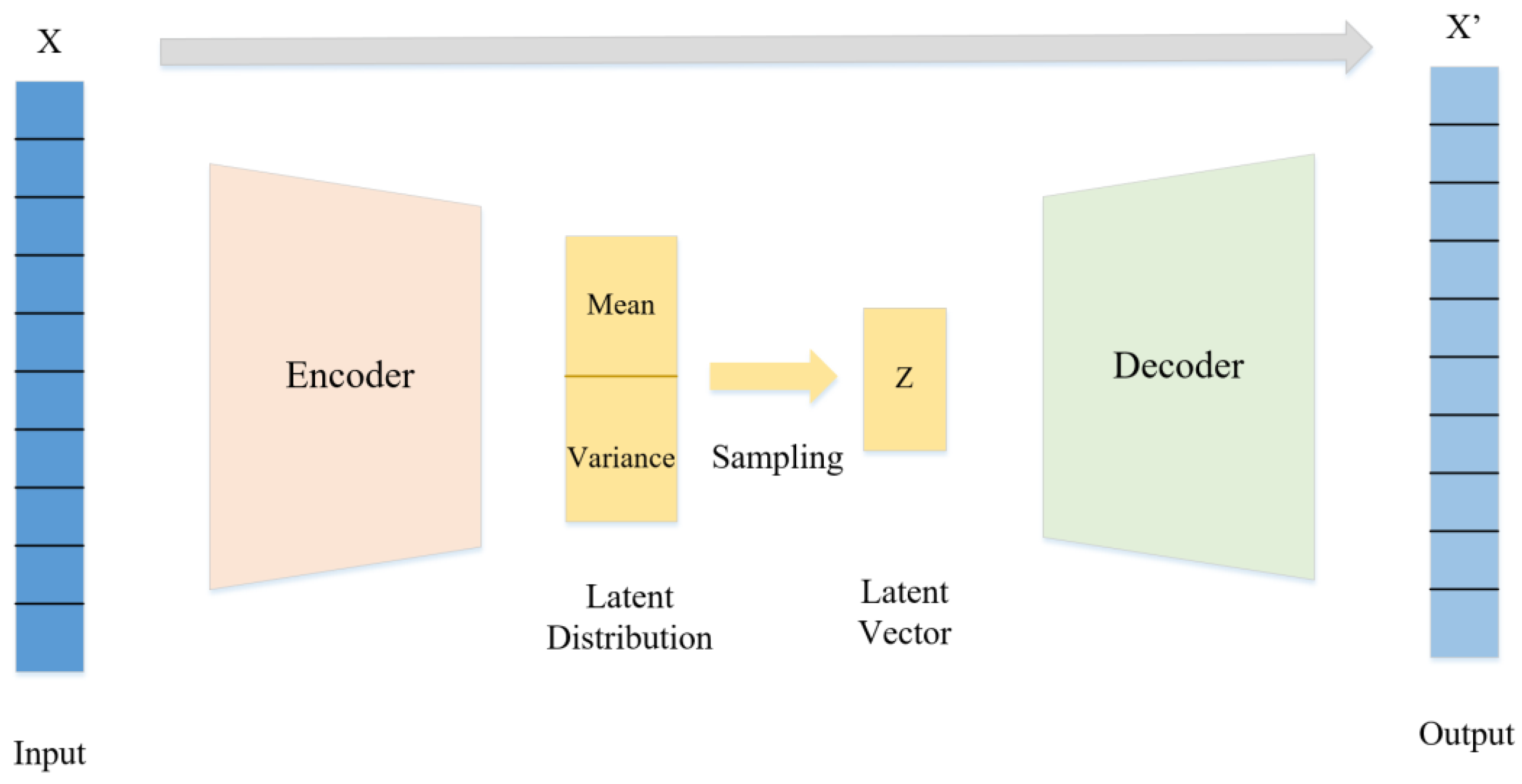
3.2. Structure of the VAE

As Figure 1 illustrates, a VAE consists of two main components: an encoder network and a decoder network. The encoder transforms the input data into a lower-dimensional latent space represented by multi-normal distributions. The Gaussian distribution is the most commonly used distribution type in VAE [23]. Every Gaussian distribution in the latent space is defined by two parameters: the mean and standard deviation, which determine the center and spread of the distribution, respectively [15]. The latent vectors, which are sampled from the multi-normal distributions in the latent space, are then passed through the decoder network to produce the final output [15]. As the multi-normal latent distributions are defined by two parameters, the mean and standard deviation, analyzing the sensitivity of these two parameters to changes in input features can provide insight into how the latent distributions will be affected by different input features. The methodology for this analysis is further explained in the following steps in Section 3.3.

3.3. Sensitivity Analysis

The essence of a sensitivity analysis is taking first-order partial derivatives of outputs with respect to inputs in a neural network. First-order partial derivative, measuring changes in an output due to changes in an input, is also known as sensitivity:

$$s_{uv}\left(x_n\right)=\frac{\partial y_u}{\partial x_v} ,$$

(1)

where $x_n$ represents the nth data sample in the dataset; and $s_{uv}$ represents the sensitivity of the uth neuron in the output layer ($y_u$) with respect to the vth neuron in the input layer ($x_v$) [19]. The notation used throughout the rest of the paper is outlined in

Table 1. Notations used in Section 3.3.

Symbol	Meaning
N	total number of data points in a dataset
M	total number of input features
H	total number of means or standard deviations in the latent space of a VAE where 2H will be the layer size
$x_n$	a random data sample
$x_m$	mth input feature
$x_o$	Other input features except mth feature
$s_m\left(x_n\right)$	sensitivity of the latent space with respect to mth input feature for the data sample $x_n$
$s_{m,\mu }\left(x_n\right)$	sensitivity of means in the latent space of a VAE with respect to mth input feature for the data sample $x_n$
$s_{m,\sigma }\left(x_n\right)$	sensitivity of standard deviations in the latent space of a VAE with respect to mth input feature for the data sample $x_n$
$s_{hm,\mu }\left(x_n\right)$	sensitivity of hth mean in the latent space of a VAE (${\mu }_h$) with respect to mth input feature for the data sample $x_n$
$s_{hm,\sigma }\left(x_n\right)$	sensitivity of hth standard deviation in the latent space of a VAE (${\sigma }_h$) with respect to mth input feature for the data sample $x_n$
$S_{m,\mu }^{sq}$	mean squared sensitivity of means in the latent space with respect to mth input feature for the entire dataset
$S_{m,\sigma }^{sq}$	mean squared sensitivity of standard deviations in the latent space with respect to mth input feature for the entire dataset
$S_{hm,\mu }^{sq}$	mean squared sensitivity of hth mean in the latent space of a VAE (${\mu }_h$) with respect to mth input feature for the entire dataset
$S_{hm, \sigma }^{sq}$	mean squared sensitivity of hth standard deviation in the latent space of a VAE (${\sigma }_h$) with respect to mth input feature for the entire dataset
$S_m^{sq}$	mean squared sensitivity of the latent space with respect to mth input feature for the entire dataset
$F_m$	relative feature importance
$c$	normalization factor
$S_m$	$s_m\left(x_n\right)$ at a local level or $S_m^{sq}$ at a global level
$i_m\left(x_n\right)$	interactions between the feature $x_m$ and other features $x_o$ for the data sample, $x_n$, in a tabular dataset
$I_m$	global interactions between mth feature and other features

.

Step 1 (Sensitivity):

To adapt a sensitivity analysis to fit into an encoder of a VAE, the sensitivity can be modified as:

$$s_{hm,\mu }\left(x_n\right)=\frac{\partial {\mu }_h}{\partial x_m} ,$$

(2)

$$s_{hm, \sigma }\left(x_n\right)=\frac{\partial {\sigma }_h}{\partial x_m},$$

(3)

where h is the index of means and standard deviations in the latent space of a VAE; m is the index of input features; $s_{hm,\mu }\left(x_n\right)$ refers to the sensitivity of hth mean in the latent space of a VAE (${\mu }_h$) with respect to mth input feature ($x_m$) for the data sample $x_n$; and $s_{hm,\sigma }\left(x_n\right)$ refers to the sensitivity of hth standard deviation in the latent space of a VAE (${\sigma }_h$) with respect to mth input feature ($x_m$) for the data sample $x_n$.

Step 2 (Local Feature Importance):

A local interpretation of each input feature refers to the case that only a single data sample in the dataset is studied. In this paper, we determine the effects of each input feature on the latent representation for a specific data sample by considering both the overall sensitivity of mean and the overall sensitivity of standard deviation with respect to each input feature:

$$\begin{array}{cc}{s}_m\left(x_n\right)& =s_{m,\mu }\left(x_n\right)+s_{m,\sigma }\left(x_n\right)\\ & ={\displaystyle {\displaystyle \sum }_{h=1}^H}\left|s_{hm, \mu }\left(x_n\right)\right|+{\displaystyle {\displaystyle \sum }_{h=1}^H}\left|s_{hm, \sigma }\left(x_n\right)\right| ,\end{array}$$

(4)

where $s_m\left(x_n\right)$ represents the sensitivity of the latent space to input feature $x_m$ for data sample $x_n$ and H is the total number of means or standard deviations in the latent space of a VAE. Taking the absolute values of $s_{hm, \mu }\left(x_n\right)$ and $s_{hm, \sigma }\left(x_n\right)$ is designed to prevent cancellation of positive sensitivity values with negative ones.

Step 3 (Global Feature Importance):

In order to obtain a global interpretation, the mean squared sensitivity introduced by Zurada et al. in 1994 is modified to fit a VAE model [24]:

$$S_{hm,\mu }^{sq}=\sqrt{\frac{{{\displaystyle \sum }}_{n=1}^N(s_{hm, \mu }{\left(x_n)\right)}^2}{N} },$$

(5)

$$S_{hm, \sigma }^{sq}=\sqrt{\frac{{{\displaystyle \sum }}_{n=1}^N(s_{hm, \sigma }{\left(x_n)\right)}^2}{N} ,}$$

(6)

where N is the total number of data points in the dataset. Equations (5) and (6) are designed to assess the sensitivity of hth mean or hth standard deviation in the latent space of a VAE with respect to mth input feature across the entire dataset.

Then, $S_{hm,\mu }^{sq}$ for different mean neurons, and $S_{hm,\sigma }^{sq}$ for different standard deviation neurons in the latent space are designed to be summed up, respectively:

$$S_{m,\mu }^{sq}={\displaystyle \sum }_{h=1}^H{S}_{hm,\mu }^{sq},$$

(7)

$$S_{m,\sigma }^{sq}={\displaystyle \sum }_{h=1}^H{S}_{hm,\sigma }^{sq}.$$

(8)

This counts the overall effects of the feature $x_m$ on means or standard deviations in the latent space of a VAE. Here, $S_m^{sq}$ is defined as representing the sensitivity of the latent space with respect to a specific input feature in this paper and can be obtained by adding the sensitivity of means in the latent space with respect to that specific feature and the sensitivity of standard deviations in the latent space with respect to that specific feature together:

$$S_m^{sq}=S_{m,\mu }^{sq}+S_{m,\sigma }^{sq}.$$

(9)

If the sensitivity $S_m^{sq}$ is close to 0, it indicates that changes in the input feature $x_m$ have a negligible impact on the outputs, meaning this input feature may be irrelevant. However, if the sensitivity $S_m^{sq}$ is significantly greater or smaller than 0, the input feature $x_m$ can be considered an important one since a minor change in this input feature might cause significant changes in outputs.

Step 4 (Relative Feature Importance):

Ranking features at a local or global level can be achieved by calculating the relative feature importance $F_m$ for each feature [20]:

$$F_m=c·S_m ,$$

(10)

where $S_m$ can be $s_m\left(x_n\right)$ at a local level and $S_m^{sq}$ at a global level and c is a normalization factor. The product of the normalization factor and the sum of the sensitivities for all features in a dataset should be equal to 100 [20]:

$$c·{\displaystyle \sum }_{m=1}^M{S}_m=100 ,$$

(11)

where M is the total number of features in a dataset so that the relative feature importance for each feature can be represented as a percentage.

Step 5 (Feature Interaction):

Most studies analyze the first-order relationship between the input and output in an MLP without further exploring the second-order effects [12]. However, a feature with a first-order partial derivative being close to zero does not necessarily mean the feature is not important. In practice, when a dataset is complex, there might exist some correlations between features, which could be measured by calculating the second-order mixed partial derivatives [12].

In VAE synthetic data generation, the interactions between the feature $x_{m,n}$ and other features for a data sample $x_n$ in a tabular dataset, can be measured by the following designed equation:

$$i_m\left(x_n\right)={\displaystyle \sum }_{o=1,o\ne m}^M{\displaystyle \sum }_{h=1}^H\left|\frac{\partial }{\partial x_m}\left(\frac{\partial {\mu }_h}{\partial x_o}\right)\right|+{\displaystyle \sum }_{o=1,o\ne m}^M{\displaystyle \sum }_{h=1}^H\left|\frac{\partial }{\partial x_m}\left(\frac{\partial {\sigma }_h}{\partial x_o}\right)\right|,$$

(12)

where $x_m$ represents the mth feature of a data sample; $x_o$ represents the oth feature of a data sample. $\frac{\partial }{\partial x_m}\left(\frac{\partial {\mu }_h}{\partial x_o}\right)$ measures the changes of the sensitivity of the mean ${\mu }_h$ in the latent space with respect to the feature $x_o$ with respect to the changes of the feature $x_m.$ Similarly, $\frac{\partial }{\partial x_m}\left(\frac{\partial {\sigma }_h}{\partial x_o}\right)$ measures the changes of the sensitivity of the standard deviation ${\sigma }_h$ in the latent space with respect to the feature $x_o$ with respect to the changes of the feature $x_m$. Recall that H is the total number of means or standard deviations in the latent space of a VAE and M is the total number of input features in a tabular dataset. Taking absolute values of the second-order partial derivative is to avoid the cancellation of positive values with negative ones. In this paper, to capture global feature interaction for each feature, the second-order derivatives are averaged across all data samples:

$$I_m=\frac{{{\displaystyle \sum }}_{n=1}^N{i}_m\left(x_n\right)}{N} .$$

(13)

If the second-order partial derivative $I_m$ is close to 0, it indicates that interactions between the feature $x_m$ and other features are weak. Changing $x_m$ will not cause the impacts of other features on the latent space to change significantly. In this case, $x_m$ can be considered an unimportant feature that can be safely removed to reduce the complexity of a dataset if the first-order partial derivative with respect to $x_m$ is close to 0 as well. The next equation will discuss how a sensitivity analysis can be applied to analyze the contributions of each input feature to the latent representation of a VAE model in practice.

3.4. Framework Design

In the area of ML, the assumption of random variables being independently and identically distributed (IID) is essential to the majority of ML models [25]. This paper assumes IID input data, as in the first VAE paper by Kingma and Welling [15]. Considering the data type being investigated in this paper is tabular data, the IID assumption allows us to only consider the relationship between column features rather than relations between data samples presented in rows.

Before applying a sensitivity analysis, input data will be normalized to avoid misleading results of extremely large or small values of partial derivatives calculated during the sensitivity analysis. As Figure 2 illustrates, the input data and the parameters that determine the latent distributions after training (means and standard deviations) will be utilized to evaluate the significance of each input feature by calculating their feature importance values using the methods outlined in Section 3.3. A feature will be considered important if its feature importance value is far away from 0. However, if a feature has a feature importance value close to 0, a feature interaction analysis, as described in Section 3.3, will be conducted to assess the interactions between this feature and other features in the dataset. If the feature interaction value is notably away from 0, then this feature is considered to be relevant due to its strong interactions with other features. Otherwise, the feature is considered to be insignificant and can be removed to reduce the complexity of the dataset as it has a minimal impact on both outputs and other features.

3.5. Experiment Preparation

To verify the robustness of the sensitivity-based method described in Section 3.3 and Section 3.4, a numerical example and three Kaggle banking datasets were utilized to show how this method can be applied to explain the importance of different inputs toward outputs.

3.5.1. Numerical Example

A numerical example where we can design the relative importance of each input feature was used to prove whether sensitivity analysis can be used to calculate feature importance. Assuming the following function:

$$Y=X_1+3X_2+X_1·X_2+5X_3-6X_4+7X_5+0.05X_6+0.01X_6·X_7 ,$$

(14)

where $Y$ represents the output generated from 7 input features from $X_1$ to $X_7$. Each input feature contains 3000 values which are randomly generated from a standard normal distribution. Hence, there are 3000 outcomes generated by 3000 data samples with each data sample made of 7 features. This example will concentrate on providing global interpretations to see if they can match the feature importance set in Equation (14).

3.5.2. Application Examples

To test the methodology outlined in Section 3.3 and Section 3.4, three real-world datasets were downloaded from an open source Kaggle, which are publicly available. This study concentrates on tabular banking data, making the tabular data as the chosen data type for examining the effect of each input feature on the latent space when VAE is used to synthesize data.

Dataset 1 comprises 10,000 rows representing various data samples (clients) and 13 columns representing different client information. This dataset is divided into two classes based on whether clients will retain their bank accounts. Dataset 2, from a marketing campaign of a Portuguese banking institution, includes approximately 41,000 data samples and 20 columns. This dataset is categorized into two classes based on whether clients will subscribe to a term deposit. Dataset 3 comprises approximately 164,000 rows and 14 columns. This dataset is grouped into 3 categories based on the customer’s interest rates for loans, 1%, 2%, and 3%. The number of data samples in each category for the three datasets is illustrated in Figure 3, Figure 4 and Figure 5.

During data preprocessing, columns, including “row number”, “customer ID number”, and “name”, are removed from the three datasets as they do not provide useful customer information. Columns with a significant amount of missing data are also dropped, which results in the total number of input features for the three datasets being 10, 19, and 11, respectively. To make the categorical features recognizable by a VAE, target encoding is used to transform them into numerical values. Lastly, to ensure that the VAE does not give more weight to larger values regardless of their unit measurements, three banking datasets are rescaled through normalization using the scikit-learn object MinMaxScaler.

Since this research focuses on using interpretability techniques to explain decisions made by an ML model rather than solely achieving optimal performance, model hyperparameters are adjusted to ensure the interpretations generated are both accurate and stable. To prevent overfitting while maintaining good learning capacity, the dimensions of input features for all three datasets were compressed to 75% of their original sizes and stored in the latent space of VAEs. Through experimentation, it was found that learning rates of 0.01 for dataset 1 and dataset 3 and 0.05 for dataset 2 work well for optimizing the VAE. The same VAE structure, consisting of a 4-layer encoder and 4-layer decoder, was used to synthesize data for three datasets. For each dataset, VAE was trained for 300 epochs. After fine-tuning the hyperparameters, the final loss values, calculated as the sum of similarity loss and KL Divergence, decreased from 71.43 to 13.48 for dataset 1, from 34.97 to 12.65 for dataset 2, and from 53.12 to 9.46 for dataset 3.

4. Results

This section provides experimental results for both the numerical and application examples.

4.1. Numerical Example Results

The sensitivities of output to each input feature (a first-order partial derivative of output Y with respect to each input feature) for each data sample were calculated. The mean squared sensitivity for each feature can be formulated by using Equation (5) or Equation (6) in Section 3:

$$S_m^{sq}=\sqrt{\frac{{{\displaystyle \sum }}_{n=1}^{3000}(s_m{\left(x_{m,n})\right)}^2}{3000} } ,$$

(15)

where $m$ ∈ {1,2,3…,7} and n ∈ {1,2,3…,3000}. Recall that $S_m^{sq}$ represents the sensitivity for each feature, and $x_{m,n}$ represents a feature of a data sample in the simulated dataset. Then the mean squared sensitivity for each feature, which can be seen in Figure 6, was multiplied by a normalization factor so that relative feature importance values sum up to 100. As Figure 7 demonstrates, the relative importance of feature $X_4$ is 1.2 times that of feature $X_3$ as anticipated. The relative importance of feature $X_5$ is 1.4 times that of feature $X_3$. The relationships between features $X_3$ and $X_5$ and the output $Y$ is linear. For features from $X_3$ to $X_5$, as the magnitude of an input feature coefficient increases, the first-order partial derivative of the input feature also increases, leading to a higher relative feature importance. Both Figure 6 and Figure 7 indicate that features $X_6$ and $X_7$ have insignificant effects on output $Y$, since values of sensitivity and relative feature importance for features $X_6$ and $X_7$ are so small they can barely be seen in the figures.

Based on the methodology described in Section 3, a second-order partial derivative test was applied to measure interactions between features. After calculating the feature interactions for all the possible pairs of features, feature interaction values for each feature with other features are illustrated in Figure 8. For example, interactions of feature $X_4$ with any other features can be calculated by using Equation (12) in Section 3:

$$M_4={\displaystyle \sum }_{o=1,o\ne 4}^8\frac{\partial }{\partial X_4}(\frac{\partial Y}{\partial X_o}) ,$$

(16)

where $M_4$ is feature interactions between $X_4$ and any other features $X_o$. As Figure 8 shows, $X_1$ and $X_2$ have the strongest interactions with others while the remaining features in Equation (14) have very weak interactions with other features. We can see the feature interaction values for $X_1$ and $X_2$ is around 1.0 while the interaction values for the rest of features are either 0 or close to 0. Since $X_6$ and $X_7$ have an insignificant impact on the output and weak interactions with other features, $X_6$ and $X_7$ can be considered as two unimportant features in this numerical example. The output, $Y$, would not be largely affected with $X_6$ and $X_7$ being removed.

4.2. Application Example Results

By applying the methodology described in Section 3, the following results were obtained. The variables on the x-axis in all figures in Section 4.2 represent different features in banking datasets 1, 2, or 3 as outlined in

Table 2. Variables on x-axis and their corresponding feature names for dataset 1.

Variable	Feature Name	Variable	Feature Name
X1	credit score	X6	balance
X2	geography	X7	number of products
X3	gender	X8	if the client has a credit card
X4	age	X9	if the client is an active member
X5	tenure	X10	estimated salary

,

Table 3. Variables on x-axis and their corresponding feature names for dataset 2.

Variable	Feature Name	Variable	Feature Name
X1	age	X11	number of contacts performed during this campaign
X2	job	X12	number of days since the client was contacted from a previous campaign
X3	marital status	X13	number of contacts performed before this campaign
X4	education	X14	outcome of previous campaign
X5	if has credit in default	X15	employment variation rate
X6	if has housing loan	X16	consumer price index
X7	if has personal loan	X17	consumer confidence index
X8	communication type	X18	Euribor 3-month rate
X9	last contact month	X19	number of employees
X10	last contact day

and

Table 4. Variables on x-axis and their corresponding feature names for dataset 3.

Variable	Feature Name	Variable	Feature Name
X1	requested loan amount	X7	debt to income ratio
X2	length of employment	X8	number of inquiries in last 6 months
X3	ownership of a house	X9	number of open accounts
X4	annual income	X10	number of total accounts
X5	if income is verified	X11	gender
X6	purpose of loan

.

The Figure 9, Figure 10, Figure 11, Figure 12, Figure 13 and Figure 14 provide local and global interpretations of feature importance in the banking datasets 1, 2, and 3. Figure 9, Figure 11 and Figure 13 display the sensitivity of the latent space with respect to each feature for a single data sample, while Figure 10, Figure 12 and Figure 14 show the sensitivity of the latent space with respect to each feature considering all the data samples. The y-axis of these figures represents local and global sensitivity values for each feature, respectively. The y-axis can also be used to represent the relative feature importance by multiplying feature importance values with a normalization factor, as described in Section 3.

For dataset 1, the feature “if the client is an active member” (X9) with the highest global importance value is found to be the most important feature for VAE to synthesize the data, which is classified based on whether the client will keep their bank accounts. However, “age” (X4) may be considered insignificant as it has the lowest global importance value close to 0. In dataset 2, “if the client has personal loan” (X7) is the most significant feature for the VAE to generate synthetic data, which is grouped based on whether the client will subscribe to a term deposit as it has a much higher global importance value than other features, while the feature “number of contacts performed during this campaign” (X11) may be considered unimportant as it has the lowest global importance value close to 0. For dataset 3, both local and global feature importance shows that “annual income” (X4) is the most important feature that has the largest impact on the latent space of the VAE to synthesize the data, which is divided based on clients’ interest rates for loans. “Requested loan amount” (X1), “length of employment” (X2), “if income is verified” (X5), and “gender” (X11) can also be considered to be significant features. However, “number of inquiries in last six months” (X8), “number of open accounts” (X9), and “number of total accounts” (X10) with feature importance values or first-order partial derivative values close to 0 may be considered as three irrelevant features in this banking dataset. In order to confirm that “age” (X4) in dataset 1, “number of contacts performed during this campaign” (X11) in dataset 2, and “number of inquiries in last 6 months” (X8), “number of open accounts” (X9), and “number of total accounts” (X10) in dataset 3 are not contributing significantly to the VAE data synthesis, a second-order partial mixed derivative test was performed to investigate interactions of each feature with the other features in the banking dataset 1, 2 or 3.

The Figure 15, Figure 16, Figure 17, Figure 18, Figure 19 and Figure 20 present feature interaction values of every feature in the banking dataset 1, 2 and 3 at the local and global level. For dataset 1, it is determined that the feature “age” (X4) is insignificant as it has a low feature importance value and minimal interaction with other features on a global scale. For dataset 2, “number of contacts performed during this campaign” (X11) is also found to have little to no interaction with other features at a global level, indicating that its removal from the dataset would not greatly affect the synthetic data generated by the VAE. For dataset 3, it is noticeable that the “number of open accounts” (X9) has strong interactions with other features in the banking dataset, as well as “number of total accounts” (X10). However, “number of inquiries in last 6 months” (X8) illustrates weak interactions with other features. Therefore, we would expect that removing “number of inquiries in last 6 months” (X8) will have a minor impact on the latent space of the VAE and the final quality of synthetic data.

5. Discussion

Through four experiments, the sensitivity-based method shows three major advantages compared with the visualization method mentioned in Section 2. First, the method can intuitively demonstrate feature importance and interaction numerically and graphically. Second, the experimental results prove that the proposed approach can provide both local and global interpretations. Third, the method is computationally inexpensive. The computational time to calculate either feature importance (first-order partial derivatives) or feature interaction (second-order partial mixed derivatives) in the application examples is on the order of seconds on a Google cloud platform. Although computational time will increase as the dataset size increases, this sensitivity-based method is still expected to explain the impacts of features on the latent space of a VAE in a very efficient way.

However, this sensitivity-based method also has some restrictions. One limitation is that after calculating the sensitivity, relative importance, and feature interaction, data scientists still need to use their domain knowledge and experience to determine threshold values for the first and second derivatives to eliminate features. Another limitation is this sensitivity-based method heavily relies on the training of a VAE, unlike TabNet which can be used as a preprocessing step to identify important features. The proposed method requires fine-tuning of VAE hyperparameters for accurate interpretations. If the latent space of a VAE fails to generalize well and extract the key information from an input dataset, interpretations may not be able to provide any useful information. In addition, the proposed method may generate different results due to factors such as random initialization, data variability and VAE hyperparameter tuning. However, these differences can be minimized by using a fixed seed for initializing the weights, stabilizing the random selection of data samples in mini-batch updates, and maintaining consistent VAE hyperparameters..

As emphasized in Section 1, the main objective of this paper was to study the impact of input features in an original tabular dataset on learning the latent representation of the tabular dataset in a VAE model, which is used to generate synthetic data. This paper concentrates on extending sensitivity analysis to assess the contributions of different features in an input dataset to the latent representation of a VAE. Below are some future work proposals.

Interpretations will have practical meanings only when a VAE model has a relatively good performance. A well-learned latent space makes interpretation results more meaningful. In the application example, the loss value may be further reduced by tuning hyperparameters to train a better latent representation. To ensure a good VAE model performance before implementing interpretability techniques, one potential research direction could be to investigate if there are any possibilities for designing a better loss function to describe the performance of a VAE model.

Since financial data usually contain sensitive information, using synthetic data to replace real data is becoming more favorable within banks. VAE is one of the most popular deep-learning models for synthesizing data [2]. Understanding how VAE generates synthetic data is important. In this context, apart from feature importance calculated by sensitivity analysis introduced in this paper, more tools or methodologies can be designed to provide additional explanations of synthetic data generation using a VAE model in the future.

The proposed method in this paper can be expanded to other industries beyond finance, such as education and healthcare, where VAE can be utilized to generate synthetic data for protecting the privacy of students and patients and obtaining more training data. In education, various Explainable AI (XAI) techniques has been applied to extract more comprehensive information from student agency data to enhance teachers’ pedagogical awareness and reflection [26]. Combining VAE with the proposed method can serve as an alternative approach to help teachers recognize and comprehend the diverse perspectives of student agency in their courses and provide suggestions for pedagogical planning while producing synthetic data. In healthcare, XAI is employed to enhance decision-making by providing physicians and patients with more accurate and interpretable predictions and recommendations [27]. The proposed method can also be used to explain the significance of different input features when VAE is used to synthesize data to mitigate privacy concerns of patients and produce more training data for ML models for a given task.

The presented work is specifically designed for the situation that latent distributions are commonly used Gaussian distributions, but the same concept behind the proposed methodology can be extended to different distributions, such as Bernoulli distributions. By determining the sensitivities of parameters that define the latent distributions to each input feature, the impact of each input feature on VAE data synthesis can be understood.

6. Conclusions

This paper proposes to use a sensitivity-based interpretation technique to assess how each input feature in a tabular dataset could impact the latent space of VAEs used to generate synthetic data. Since synthetic data is generated based on the latent space of a VAE model, knowing the contributions of each feature towards the latent representation helps us better understand what features are more heavily relied on to generate synthetic data. The contributions and relative importance of a feature can be measured by taking first-order partial derivatives of the outputs of an encoder with respect to the input feature. If a feature has a first-order partial derivative far away from zero, then this feature is an important one. Suppose a feature has a first-order partial derivative close to zero. This indicates the feature may not be significant since this feature has a negligible impact on the outputs of the encoder, which are means and standard deviations in the latent space. To filter irrelevant features from a dataset, second-order partial derivatives need to be performed to check the interactions between the features considered unimportant in the first-order partial derivative test and other features. Only features with low feature importance and weak feature interactions with other features can be removed from a dataset. The four experiments in Section 3 and Section 4 demonstrate this sensitivity-based method can provide explanatory insights into the contributions of each input feature in a tabular dataset on the latent space by identifying essential features and discovering relationships between input features.

References

1. Alabdullah, B.; Beloff, N.; White, M. Rise of Big Data–Issues and Challenges. In Proceedings of the 2018 21st Saudi Computer Society National Computer Conference (NCC), Riyadh, Saudi Arabia, 25–26 April 2018; pp. 1–6. [Google Scholar] [CrossRef]
2. Assefa, S.A.; Dervovic, D.; Mahfouz, M.; Tillman, R.E.; Reddy, P.; Veloso, M. Generating synthetic data in finance: Opportunities, challenges and pitfalls. In Proceedings of the First ACM International Conference on AI in Finance, New York, NY, USA, 15–16 October 2020; pp. 1–8. [Google Scholar] [CrossRef]
3. Tucker, A.; Wang, Z.; Rotalinti, Y.; Myles, P. Generating high-fidelity synthetic patient data for assessing machine learning healthcare software. NPJ Digit. Med. 2020, 3, 147. [Google Scholar] [CrossRef] [PubMed]
4. Joseph, A. We need Synthetic Data. Available online: https://towardsdatascience.com/we-need-synthetic-data-e6f90a8532a4 (accessed on 26 March 2022).
5. Christoph, M. How do You Generate Synthetic Data? Available online: https://www.statice.ai/post/how-generate-synthetic-data (accessed on 26 March 2022).
6. Mi, L.; Shen, M.; Zhang, J. A Probe Towards Understanding GAN and VAE Models. arXiv 2018, arXiv:1812.05676. [Google Scholar] [CrossRef]
7. Singh, A.; Ogunfunmi, T. An Overview of Variational Autoencoders for Source Separation, Finance, and Bio-Signal Applications. Entropy 2022, 24, 55. [Google Scholar] [CrossRef] [PubMed]
8. van Bree, M. Unlocking the Potential of Synthetic Tabular Data Generation with Variational Autoencoders. Master’s Thesis, Tilburg University, Tilburg, The Netherlands, 2020. [Google Scholar]
9. Shankaranarayana, S.M.; Runje, D. ALIME: Autoencoder Based Approach for Local. arXiv 2019, arXiv:1909.02437. [Google Scholar] [CrossRef] [Green Version]
10. Xu, F.; Uszkoreit, H.; Du, Y.; Fan, W.; Zhao, D.; Zhu, J. Explainable AI: A Brief Survey on History, Research Areas, Approaches and Challenges. In Natural Language Processing and Chinese Computing, Proceedings of the 8th CCF International Conference, NLPCC, Dunhuang, China, 9–14 October 2019; Springer International Publishing: Manhattan, NY, USA, 2019; Volume 11839, pp. 563–574. [Google Scholar] [CrossRef]
11. Bengio, Y.; Courville, A.; Vincent, P. Representation Learning: A Review and New Perspectives. arXiv 2013, arXiv:1206.5538. [Google Scholar] [CrossRef] [PubMed] [Green Version]
12. Yeh, I.-C.; Cheng, W.-L. First and second order sensitivity analysis of MLP. Neurocomputing 2010, 73, 2225–2233. [Google Scholar] [CrossRef]
13. Shah, C.; Du, Q.; Xu, Y. Enhanced TabNet: Attentive Interpretable Tabular Learning for Hyperspectral Image Classification. Remote Sens. 2022, 14, 716. [Google Scholar] [CrossRef]
14. Arik, S.Ö.; Pfister, T. TabNet: Attentive Interpretable Tabular Learning. arXiv 2020, arXiv:1908.07442. [Google Scholar] [CrossRef]
15. Kingma, D.P.; Welling, M. Auto-Encoding Variational Bayes. arXiv 2014, arXiv:1312.6114. [Google Scholar] [CrossRef]
16. Spinner, T.; Körner, J.; Görtler, J.; Deussen, O. Towards an Interpretable Latent Space. In Proceedings of the Workshop on Visualization for AI Explainability, Berlin, Germany, 22 October 2018. [Google Scholar]
17. Seninge, L.; Anastopoulos, I.; Ding, H.; Stuart, J. VEGA is an interpretable generative model for inferring biological network activity in single-cell transcriptomics. Nat. Commun. 2021, 12, 5684. [Google Scholar] [CrossRef] [PubMed]
18. Fortuin, V.; Hüser, M.; Locatello, F.; Strathmann, H.; Rätsch, G. Som-vae: Interpretable discrete representation learning on time series. arXiv 2019, arXiv:1806.02199. [Google Scholar] [CrossRef]
19. Pizarroso, J.; Pizarroso, J.; Muñoz, A. NeuralSens: Sensitivity Analysis of Neural Networks. arXiv 2021, arXiv:2002.11423. [Google Scholar] [CrossRef]
20. Mison, V.; Xiong, T.; Giesecke, K.; Mangu, L. Sensitivity based Neural Networks Explanations. arXiv 2018, arXiv:1812.01029. [Google Scholar] [CrossRef]
21. Saarela, M.; Jauhiainen, S. Comparison of feature importance measures as explanations for classification models. SN Appl. Sci. 2021, 3, 272. [Google Scholar] [CrossRef]
22. Terence, S. Understanding Feature Importance and How to Implement it in Python. Available online: https://towardsdatascience.com/understanding-feature-importance-and-how-to-implement-it-in-python-ff0287b20285 (accessed on 26 March 2022).
23. Kingma, D.P.; Welling, M. An Introduction to Variational Autoencoders. Found. Trends R Mach. Learn. 2019, 12, 307–392. [Google Scholar] [CrossRef] [Green Version]
24. Zurada, J.M.; Malinowski, A.; Cloete, I. Sensitivity analysis for minimization of input data dimension for feedforward neural network. In Proceedings of the IEEE International Symposium on Circuits and Systems-ISCAS’94, London, UK, 30 May–2 June 1994; Volume 6, pp. 447–450. [Google Scholar] [CrossRef]
25. Chandran, S. Significance of I.I.D in Machine Learning. Available online: https://medium.datadriveninvestor.com/significance-of-i-i-d-in-machine-learning-281da0d0cbef (accessed on 26 March 2022).
26. Saarela, M.; Heilala, V.; Jääskelä, P.; Rantakaulio, A.; Kärkkäinen, T. Explainable student agency analytics. IEEE Access 2021, 9, 137444–137459. [Google Scholar] [CrossRef]
27. Linardatos, P.; Papastefanopoulos, V.; Kotsiantis, S. Explainable AI: A Review of Machine Learning Interpretability Methods. Entropy 2021, 23, 18. [Google Scholar] [CrossRef] [PubMed]
Figure 1. Architecture of the Variational Autoencoder (VAE).
Algorithms 16 00121 g001
Figure 2. Flow chart of applying sensitivity analysis to interpret VAE.
Algorithms 16 00121 g002
Figure 3. Distribution of dataset 1.
Algorithms 16 00121 g003
Figure 4. Distribution of dataset 2.
Algorithms 16 00121 g004
Figure 5. Distribution of dataset 3.
Algorithms 16 00121 g005
Figure 6. Sensitivity values for simulated data.
Algorithms 16 00121 g006
Figure 7. Relative feature importance for simulated data.
Algorithms 16 00121 g007
Figure 8. Feature interaction for simulated data.
Algorithms 16 00121 g008
Figure 9. Local feature importance values for dataset 1.
Algorithms 16 00121 g009
Figure 10. Global feature importance values for dataset 1.
Algorithms 16 00121 g010
Figure 11. Local feature importance values for dataset 2.
Algorithms 16 00121 g011
Figure 12. Global feature importance values for dataset 2.
Algorithms 16 00121 g012
Figure 13. Local feature importance values for dataset 3.
Algorithms 16 00121 g013
Figure 14. Global feature importance values for dataset 3.
Algorithms 16 00121 g014
Figure 15. Local feature interaction values for dataset 1.
Algorithms 16 00121 g015
Figure 16. Global feature interaction values for dataset 1.
Algorithms 16 00121 g016
Figure 17. Local feature interaction values for dataset 2.
Algorithms 16 00121 g017
Figure 18. Global feature interaction values for dataset 2.
Algorithms 16 00121 g018
Figure 19. Local feature interaction values for dataset 3.
Algorithms 16 00121 g019
Figure 20. Global feature interaction values for dataset 3.
Algorithms 16 00121 g020