1. Introduction
Ethiopia is one of the countries in East Africa that is threatened by water scarcity. In Ethiopia, rainfed agriculture and small farming predominate. A recent study showed that around 95% of the agricultural areas in Ethiopia are rainfed areas [
1]. A Food and Agriculture Organization (FAO) study [
2] showed that small farming families make up 72% of the total population. In total, 74% of Ethiopia’s farmers come from small farming families, and 67% of these live below the national poverty line. About 75% of farmland is devoted to cereals. Maize and wheat dominate, complemented by teff, barley, sorghum, and rice. Drought is a major stressor that reduces cereal yields. Moreover, climate change has induced significant and erratic deviations in rainfall patterns over the year and across the country, significantly reducing crop yields overall, especially cereals [
3]. To mitigate the impact of water stress and reduce hunger, utilizing groundwater by drilling wells for irrigation is a potential solution to address the problem of increasingly erratic rainfall.
Predictions of groundwater level, or the depth to water table, could support decisions on where to drill wells to extract groundwater. Artificial intelligence (AI) has been widely used to predict both the surface [
4,
5,
6,
7,
8,
9,
10] and groundwater [
11,
12,
13,
14,
15,
16,
17,
18,
19,
20,
21] levels globally. Regarding surface water level prediction, Khan and Coulibaly [
4] used a Support Vector Machine (SVM) to examine the long-term water level in Lake Erie in North America based on mean monthly water level data from 1918 to 2001. The authors compared SVM with a multilayer perceptron (MLP) and with a conventional multiplicative seasonal autoregressive model. They found that the SVM outperformed the other two models with an overall RMSE of less than 0.25 m. Liang et al. [
5] applied SVM and a deep learning model based on a Long Short-Term Memory (LSTM) network to predict daily surface water levels in Dongting Lake in China. They found that the LSTM has better accuracy than the SVM model with less than 0.1 m RMSE. A river water level study performed by Chen and Qiao in 2021 [
6] also confirms that LSTM has good performance in predicting surface water levels. Choi et al. [
7] used four machine learning algorithms, including artificial neural networks (ANN), decision tree, random forest (RF), and SVM based on the daily water level from 2009 to 2013, to predict water levels from 2013 to 2015 in Upo wetlands, South Korea. They found that random forest outperformed the other three algorithms, with a 0.09 RMSE.
Regarding groundwater level prediction, in 2013, Sahoo and Jha [
11] constructed seventeen site-specific AI models to predict groundwater levels in Japan. Compared to multiple linear regression (MLR) models, ANN-predicted groundwater levels have a better agreement with RMSE values, ranging from 0.04 to 0.4 m for 17 sites. Sahoo et al. [
12] developed a modeling framework using Multilayer Perceptron (MLP) network architecture to simulate groundwater level changes in two agricultural regions in the US. They found ANN performed better than the MLR and multivariate nonlinear regression model with RMSE less than 2 m for both the agricultural regions. Zhang et al. [
13] developed a new model based on LSTM to predict groundwater levels, which outperformed feed-forward neural networks and double LSTM with a 0.14 m RMSE. In 2021, Liu et al. [
14] applied SVM combined with the data assimilation (DA) technique for predicting changes in groundwater level. The researchers predicted the change in groundwater levels at 1- to 3-month time scales for 46 wells located in the northeast United States and found that both the SVM and SVM with DA can adequately predict groundwater levels with RMSE less than 4 m. Hikouei et al. [
15] demonstrated that Extreme Gradient Boosting exhibited superior performance over the RF model for predicting groundwater levels in the tropical peatlands of Indonesia. Many recent studies employed wavelet-transformed analysis [
16,
17] and hybrid AI techniques [
18,
19], which had good performance in groundwater level prediction using time series data. Missing values in groundwater level time series datasets are a frequent occurrence, presenting challenges for accurate forecasting. To address this data gap, previous studies have utilized machine learning frameworks to estimate the missing values in groundwater level data, resulting in enhanced prediction reliability [
22,
23]. Overall, these groundwater level studies provide valuable insights into groundwater dynamics and contribute to more effective resource management.
Most of these studies that use machine learning algorithms employed a large amount of time series data to predict future water levels for lakes [
4,
5,
8], rivers [
6,
9,
10], wetlands [
7], basins [
11,
17,
19], regions [
13,
16,
18,
20], aquifers [
12], and watersheds [
14,
21]. These models generally have good performance with low mean square errors in predictions of water levels. These studies were conducted in regions with high data availability on both the time series of water level data and climate variables. Even when missing values occurred, extensive data availability greatly facilitated the estimation of data gaps [
22,
23]. However, in many regions of interest, a large amount of time series of water level data are unlikely to be available due to the high cost of data collection for local governments or organizations. Many water scarcity areas have a great need for groundwater development for sustainable irrigation, although the lack of good data can make models perform poorly. To the best of our knowledge, there is no research on groundwater level prediction using machine learning based on non-time series data in rainfed agricultural regions. It is much more difficult to predict water levels accurately in the absence of time series data because previous water level is a strong predictor of current water level.
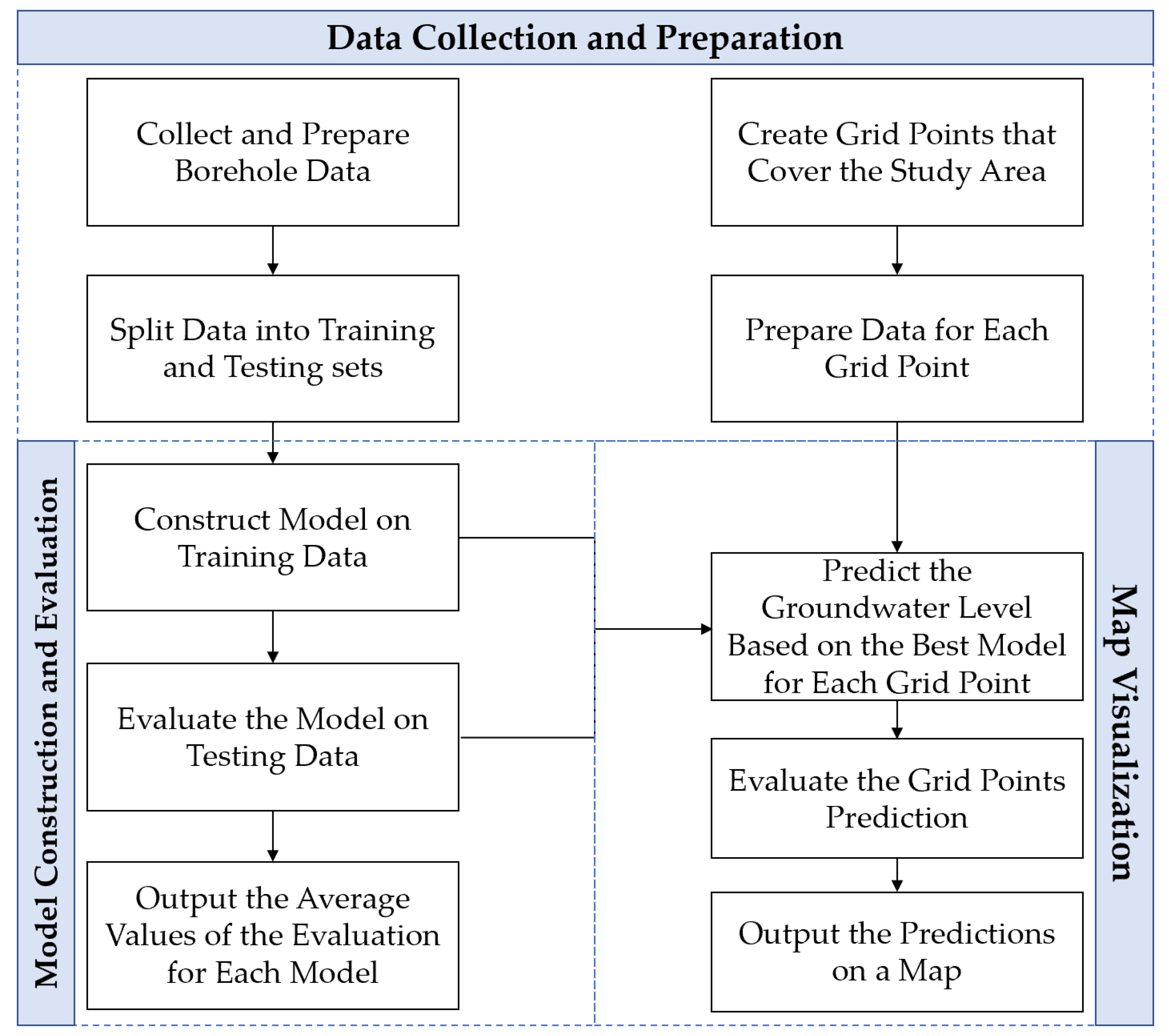
The objective of this study is to use AI to identify suitable drilling locations for sustainable irrigation for subsistence agriculture in water scarcity regions using sparse non-time series data on existing wells. To achieve this objective, five machine learning models were constructed to predict groundwater levels. These include MLR, multivariate adaptive regression splines (MARS), ANN, random forest regression (RFR), and gradient boosting regression (GBR). The models were developed using data from 75 existing boreholes in the Bilate watershed in southern Ethiopia. The best-performing model was used to predict the groundwater level for hundreds of thousands of grid points covering the Bilate region. Finally, a map of predicted water levels was created to provide guidance for decision-making on drilling locations for local individuals and organizations.
Figure 1 shows the workflow of this study.
The rest of the paper is organized as follows.
Section 2 describes the study area, data sources, and methodology used in this study;
Section 3 shows the main results from each of the machine learning models;
Section 4 provides a discussion of the results; and
Section 5 concludes the paper.
2. Materials and Methods
2.1. Study Area
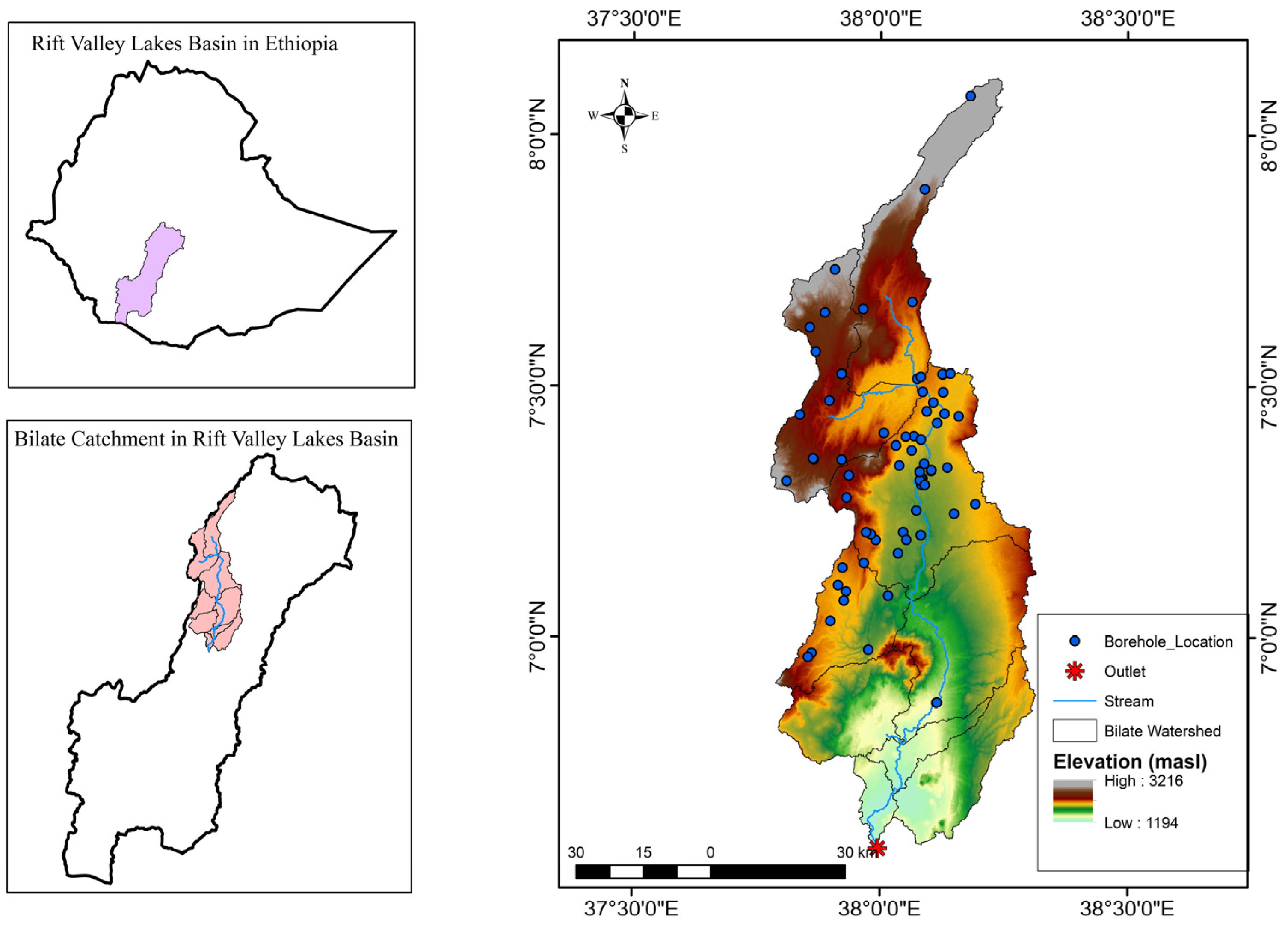
The Bilate watershed is located in southeastern Ethiopia at latitude 6°34′ to 8°6′ N and longitude 37°46′ to 38°18′ E. The total area is 5276.25 km
2. Bilate is one of the largest watersheds in the Ethiopia Rift Valley Basin [
24,
25]. Elevation of the region ranges from 1194 m to 3216 m, as shown in
Figure 2. The Bilate region was classified as a three-season climate type, with major rains from June to September, dry season from October to January, and minor rains from February to May [
26,
27]. In Bilate, the minor rains typically start in March. However, for our analysis, we adhered to the general classification, commencing from February, as referenced in [
24,
25]. The annual average precipitation within the Bilate watershed spans from 769 mm in lower regions to 1339 mm in the highlands. Meanwhile, the mean annual temperature fluctuates between 11 °C and 22 °C in Hossana, situated upstream, and ranges from 16 °C to 30 °C at Bilate Tena, the lower stream of the watershed [
24].
The vegetation density in Bilate can be generally described as sparse to dense vegetation in the minor and major rainy seasons, and sparse vegetation in the dry season. Land in the region is mainly cultivated, grassland, plantation, shrubland, and wetland. The northern and western parts of the study area are mountainous, whereas the southern and eastern parts are lowlands. Distributed lakes in the study area indicate the presence of shallow groundwater. Pyroclastic and volcano-sedimentary rocks are dominant outcrops in the study area. The productivity of the aquifers varies from moderately productive to highly productive with an average transmissivity range between 1.03 × 10
−5 and 2.78 × 10
−1 m/s
2 [
28].
Figure 2.
Bilate watershed (pink region on the lower left plot) belongs to a basin called Rift Valley (light green basin on the upper left plot). The map of Bilate watershed with boreholes and elevation [
29] is shown on the right.
Figure 2.
Bilate watershed (pink region on the lower left plot) belongs to a basin called Rift Valley (light green basin on the upper left plot). The map of Bilate watershed with boreholes and elevation [
29] is shown on the right.
2.2. Data Description
In this study, the dependent variable is the static water level. Field data on 75 boreholes were collected by Arba Minch Water Technology Institute (AWTI) in 2007 [
30]. Although the dataset was collected fifteen years ago, changes in static water level during the intervening years would have very little impact on our analysis. Any change would likely be within a few centimeters, which is small in relation to the accuracy of our analysis. Therefore, the existing historical dataset is useful to demonstrate the value of machine learning for predicting water levels.
Initially, we explored a broader range of variables, identifying a subset that demonstrated greater influence on our predictions. The method we employed for feature selection involved a synergistic approach that combined domain expertise—where we incorporated factors known to be critical in our field—with a backward stepwise feature selection using random forest regression, which iteratively removed the least significant variables based on mean square error criteria on the out-of-bag samples. This directed our attention towards incorporating this subset, resulting in the consideration of twenty independent variables for our modeling and analysis. These included elevation, soil type, meteorological variables (i.e., precipitation, specific humidity, wind speed, and land surface temperature (LST) at day and night time) and vegetation (i.e., NDVI) for the three seasons from October 2005 to September 2007. We chose to use data from a time period that closely aligned with when the static water level was measured. We had the coordinates for each of the 75 boreholes and have extracted the values for each variable from the raw dataset. Given that the resolution varied for different independent variables, borehole points that were close to each other might have the same extracted value, particularly for predictors with sparse resolution. Details on the sources of the dependent and independent variables are summarized in
Table 1 and
Table 2.
Nearly all the borehole points in the data set are located in areas categorized as cultivation or grassland. As mentioned, the purpose of this study is to predict groundwater levels to support decision-making on the optimal borehole drilling locations for agricultural irrigation. Based on the local conditions, it is unusual to place a borehole in a forest, wetland, or shrubland. For this reason, only observations in cultivated and grassland areas were included in the training and testing data sets, and the model does not predict groundwater levels for the forest, wetland, and shrubland.
Machine learning models were built using a training dataset consisting of 63 randomly selected observations. Performance was then evaluated on a testing set made up of the remaining 12 observations. Each algorithm was subjected to fifteen individual experiments. For MLR and MARS, models were constructed based on fifteen diverse and randomly selected training sets. For ANN, RFR, and GBR, five different random data separations were used, and three experiments were carried out for each training dataset. Performing a variety of experiments is important to verify the model’s ability to effectively generalize to unseen data. This paper mainly presents and discusses models with median performance. The model comparisons are based on consistent training and testing data separations across all algorithms. The average performance scores from the fifteen experiments are also reported, providing a comprehensive understanding of each model’s effectiveness.
To predict groundwater levels for a larger area in the Bilate region, we generated a grid with a resolution 100 m × 100 m that covered the Bilate region. The data for twenty independent variables for each grid point were prepared and processed in the same manner as for the original dataset of 75 boreholes. As the resolution of the grid points was relatively high, grid points that fell within the same spatial resolution unit of a variable would have identical extracted values. The primary software tools used for data preparation and visualization were QGIS 3.24.1 [
37] and R 4.1.3 [
38].
2.3. Resampling Methods
2.3.1. Leave-One-Out Cross-Validation
Cross-validation (CV) is a resampling technique to check the generalization ability of a model on a limited sample. The k-fold CV method randomly divides the observations into k groups/folds of approximately equal size [
39]. The first fold is used as the validation set. The remaining folds are used to fit a model. This process repeats k times, and a different fold is used as the validation set each time. The CV estimate is finally computed as the average of the mean square error on each validation set. Leave-one-out CV (LOOCV) is a special case of cross-validation, where k is the number of samples [
39]. In LOOCV, the model is fit based on the entire dataset with one observation excluded. Next, the fitted model is used to predict the one observation that was left out. Then, the process is repeated n times, leaving out a different observation each time, where n is the number of observations in the data set. As the dataset is small, we performed LOOCV across the machine learning models in this study.
2.3.2. Bootstrapping
Bootstrapping is a resampling method that randomly samples values with replacements. It is mainly employed in the construction of RFR models. In the context of RFR, each decision tree within the forest is trained on a distinct dataset, generated by bootstrapping the original training set. This ensures each dataset is of the same size as the original, but composed of a subset of the original data, with some samples likely repeated. This process introduces randomness into the model-building phase, which aids in preventing overfitting and improves model robustness by ensuring that each individual tree within the forest learns from a slightly different sample of the data.
2.4. Machine Learning Algorithms
Machine learning is a branch of AI focused on building systems that learn from data. It has been widely applied in science and engineering. Application areas include hydrogeology [
11,
12,
13,
14,
15,
16,
17,
18,
19,
20,
21,
22,
23,
40], cyber security [
41,
42], transportation [
43,
44], and aerospace engineering [
45,
46,
47]. By identifying patterns in data, the computer can learn a decision rule from data without explicit programming. Over time, with more data, machine learning models can make increasingly accurate predictions or decisions.
2.4.1. Multiple Linear Regression
A multiple linear regression model [
48] was built to identify factors that affected the groundwater level and, therefore, to estimate the groundwater level. The general form of a linear regression model was defined as:
where
is the intercept;
are the coefficients; and
are the predictors. The coefficients
are estimated from the training data to optimize a measure of fit, typically the sum of squared residuals.
2.4.2. Multivariate Adaptive Regression Spline
MARS is a nonparametric regression method that creates a piece-wise linear model so that the relationship between the predictor and the response can be different for different ranges of predictors [
49]. The model begins with a simple constant model and iteratively adds basis functions that best reduce the sum of squared residuals. The basis functions are created using hinge functions that form piecewise linear relationships. A hinge function takes a single variable and a constant as input, returning the difference between the variable and the constant when the variable is greater than the constant, and zero otherwise. For a cut point a, a pair of hinge functions are defined as:
where x is a given variable. Each time a pair of basis functions is added, the model chooses the variable and the constant that minimize the residual sum of squares (RSS). In order to control overfitting, MARS then performs a backward deletion process. It removes basis functions that contribute the least to the model’s predictive power based on the generalized cross-validation (GCV) score or Akaike Information Criterion (AIC) score. The backward pass prunes the model by eliminating the terms one by one until the best subset is found for the model. The one with the lowest GCV or AIC score is usually chosen as the final model.
2.4.3. Artificial Neural Networks
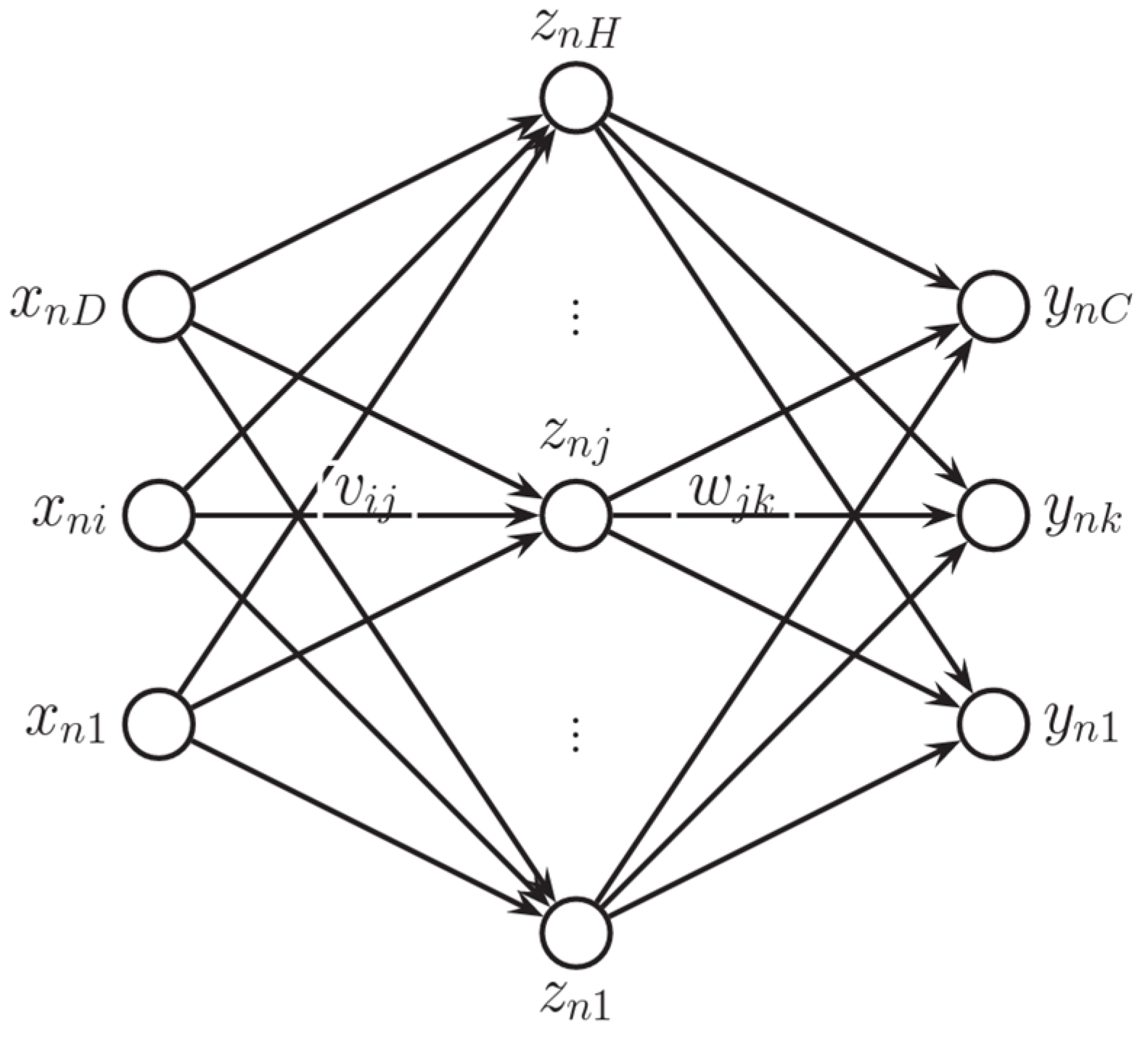
ANN is a machine-learning model inspired by the neural structure of the brain. An ANN model transforms inputs into outputs through a series of hidden layers to an output layer. For a regression model with a single hidden layer, the form of the ANN model [
50] is defined as:
where g is a non-linear activation function; z(x) is the hidden layer, which is a deterministic function of the input; H is the number of hidden units; V is the weight matrix from the inputs to the hidden nodes; and w is the weight vector from the hidden nodes to the output.
Figure 3 shows a simple neural network with only one hidden layer. The weights are typically estimated through an iterative procedure that finds a local minimum of a goodness of fit measure, typically the sum of squared residuals.
2.4.4. Random Forest Regression
The random forest regression algorithm, proposed by Breiman in 2001, is a supervised learning algorithm that produces a forecast based on many decision trees [
51]. Each tree is built based on a bootstrap sample of the training data. At each decision node of each tree, the best split is chosen among the number of randomly selected predictors. The splitting process terminates at a leaf node when a termination criterion is met. To make a prediction at a point, the tree is traversed to find the leaf node corresponding to the independent variables corresponding to the point, and the dependent variables for the data points at the leaf nodes are averaged [
52]. This procedure, creating decision trees based on different bootstrap samples and then averaging the predictions from all the trees, is called bootstrap aggregation, or bagging.
The bagging technique in the RFR model tends to reduce the variance of predictions, but a bias still exists. Specifically, as the prediction is the average of the output from all leaf nodes, observations with small values tend to be overestimated and those with large values tend to be underestimated. This tendency to bias has been identified in previous studies [
53,
54]. Our results showed a bias in the initial RFR model. To correct the bias, a post-processing bias-correcting transformation to the RFR predictions was made [
54]. For the linear transformation, a linear regression model was fitted to find the intercept (β
0) and slope (β
1) of the transformed prediction:
where ŷ is the predicted response value by the initial random forest model on training data; β
0 is the coefficient for the intercept, and β
1 is the coefficient for ŷ. The objective is to find the parameters that minimize the mean square error:
2.4.5. Gradient Boosting Regression
Gradient boosting regression (GBR) is an ensemble learning algorithm that combines multiple weak prediction models, typically decision trees, to create a strong predictive model. Initially, the ensemble is empty. The model starts with an initial prediction, typically the mean of the response variable. The difference between the observed values and the initial prediction, known as the residuals, is calculated. These residuals represent the errors that the model needs to correct. Then, a decision tree is trained to predict the residuals. The tree is constructed to minimize a specific loss function using gradient descent optimization. The loss function we used in this study is defined as:
where
is the i
th observed value;
is the predicted response value; and n is the number of observations. Next, the predictions from the decision tree are combined with the current ensemble’s predictions to obtain an updated prediction. This updated prediction is added to the ensemble. Then, the residuals are recalculated using the updated predictions. The new residuals represent the errors that were not captured by the current ensemble. The process continues for a specified number of iterations or until a certain stopping criterion is met. The final prediction is obtained by summing the predictions from the entire ensemble. By iteratively correcting the errors of the previous models, gradient boosting regression is able to learn complex relationships and improve predictive accuracy.
2.5. Evaluation Metrics
The evaluation metrics presented in this paper include mutual information (MI), root mean square error (RMSE), median absolute error (MAE), and R-squared. In the definitions below, denotes the observed value; denotes the predicted value; and denotes the mean of the observed values.
MI measures the degree of relatedness between the datasets [
55]. A higher MI value shows that the dependent variable (y) has higher relatedness to the corresponding independent variable (x).
where p(x, y) represents the joint probability function of x and y; p(x) and p(y) are the marginal probability functions of x and y, respectively.
RMSE describes how far the predictions deviate from the actual values. A small RMSE represents a good performance of the model.
MAE measures the median of absolute errors between the predicted and observed values. Similar to RMSE, it is also used to describe how well the data fit the model.
R-squared represents how much variation for a dependent variable is explained by an independent variable.
3. Results
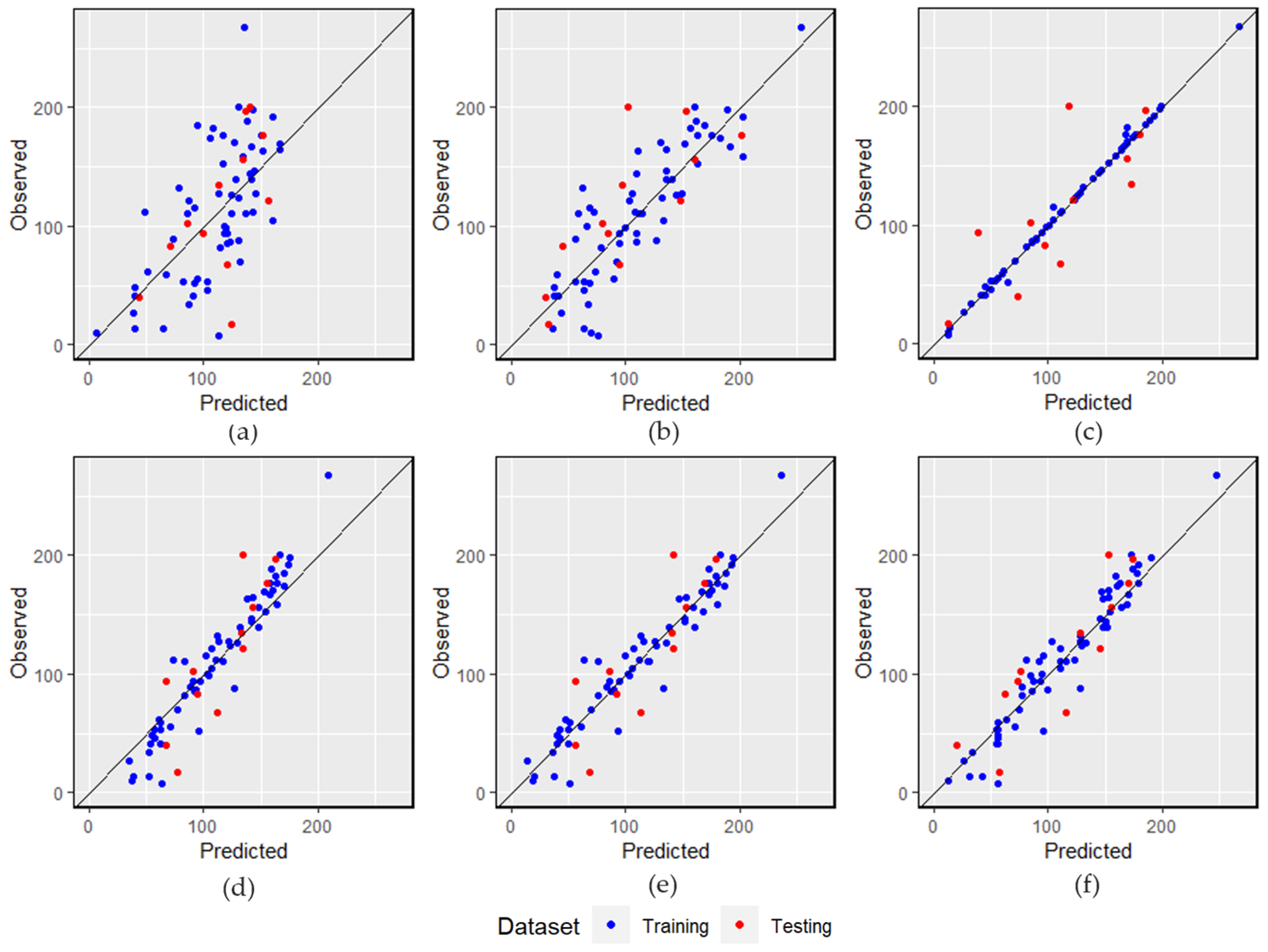
In this section, we detail the mutual information analysis and outcomes from all the implemented methods. We primarily focus on results from one training and testing data partition used consistently across all methods. This training and testing split was chosen because it yielded close to median performance across all models. For the ANN, RFR, and GBR methods, three experiments were conducted for each data partition; of these, the models with median performance were selected. Primary results associated with all algorithms include plots of residuals versus predicted values and observed versus predicted values for both training and testing data. Furthermore, tables are presented summarizing the performance metrics of the models. These include results based on a single experiment with median performance, as well as average scores across the fifteen experiments.
3.1. Mutual Information Analysis
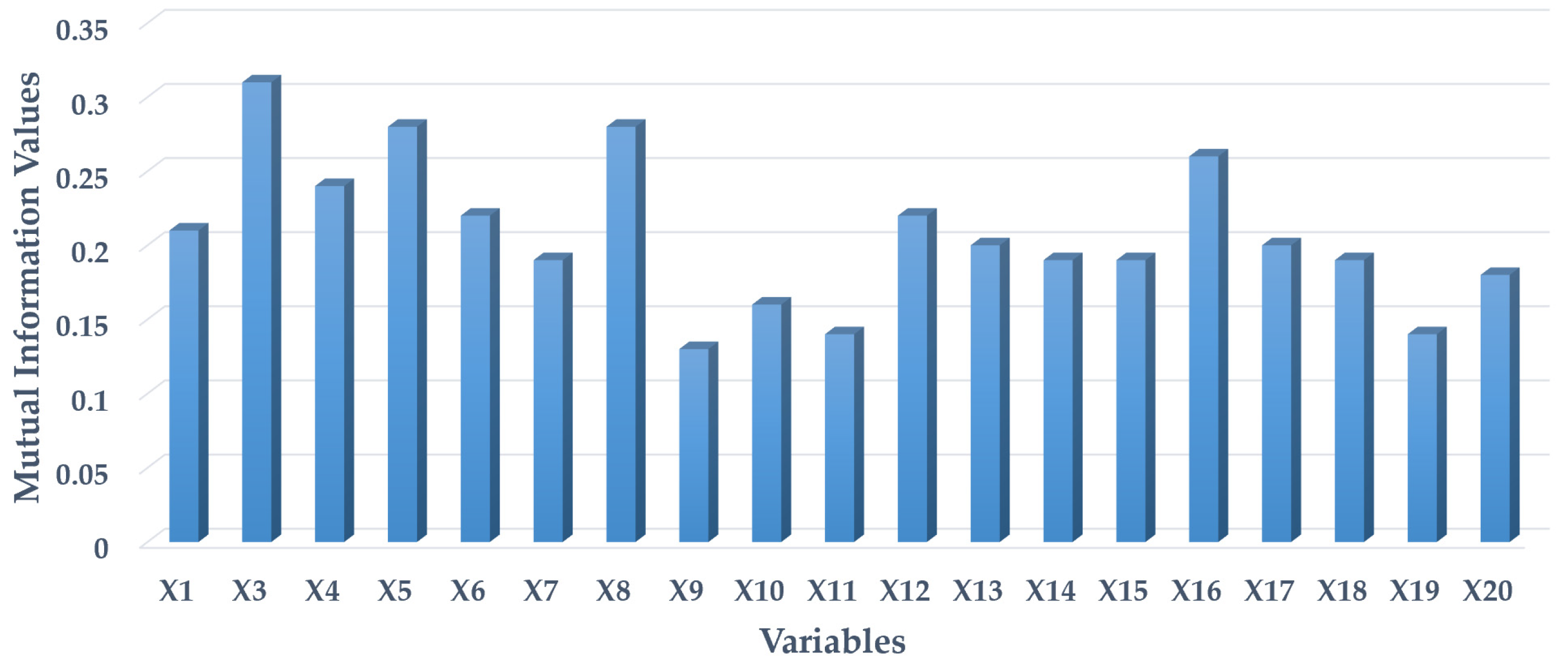
A zero MI value indicates no mutual dependence or relatedness between the specific independent variable and the static water level. A larger MI value represents a stronger relatedness.
Figure 4 shows that the variables precipitation Oct to Jan (X3), precipitation Jun to Aug (X5), and specific humidity Jun to Sep (X8) have relatively stronger relatedness to static water level. On the other hand, Wind speed Oct to Jan (X9), Wind speed Jun to Sep (X11), and NDVI Feb to May (X19) showed weaker relatedness. The soil type (X2) is removed from the mutual information analysis because it is a categorical variable.
3.2. Multiple Linear Regression
Before building the MLR, highly correlated predictors were removed. If a pair of predictors have a correlation equal to or greater than 0.85, the R function
findCorrelation() randomly picks one predictor to remove. The remaining predictors include soil type (X2), precipitation (X3–5), wind speed from Feb to May (X10), LST at daytime from Feb to May (X13), LST at nighttime from Oct to Jan (X15), NDVI from Feb to May (X19), and NDVI from Jun to Sep (X20).
Table 3 shows the predictors remaining after removal along with their coefficients. We found the factors, including the euric vertisols soil type (X2) and NDVI from Jun to Sep (X20), had a significant relationship with the static water level at a 0.05 significance level.
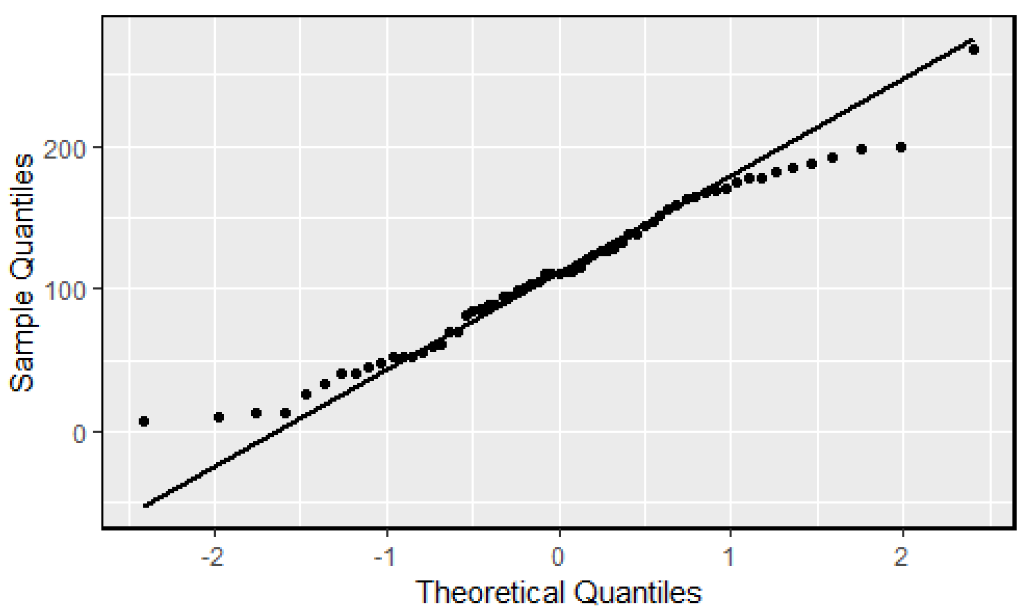
To examine the normality assumption of a linear regression model, we created a Quantile–Quantile (Q–Q) plot and a residual plot. The Q–Q plot shown in
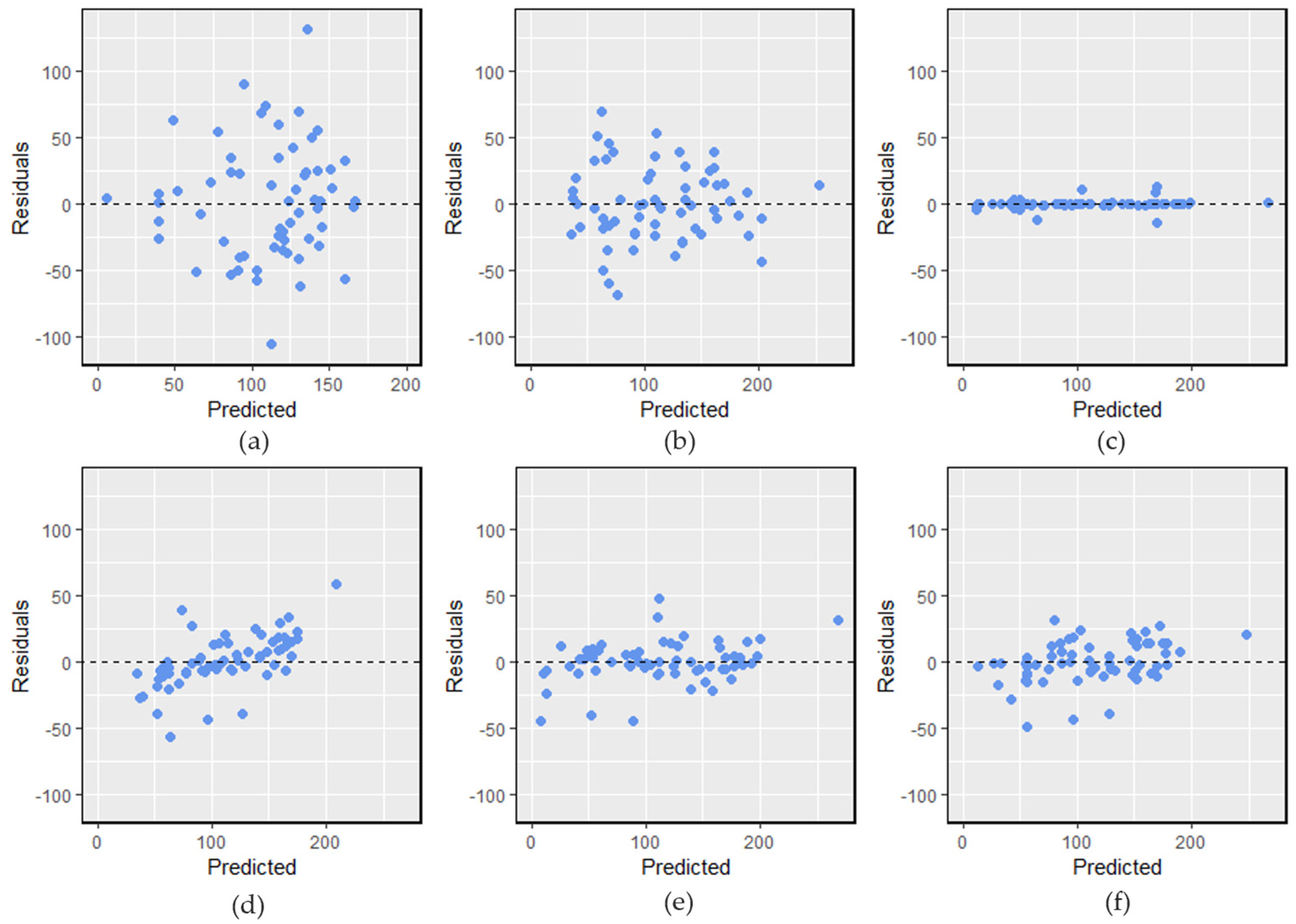
Figure 5 shows that the points are approximately distributed along the line with light upper and lower tails. No evident pattern was found on the residual plot (
Figure 6a). We also performed a Shapiro–Wilk normality test on residuals with the null hypothesis that the residuals are normally distributed. The
p-value is approximately 0.51, which is much greater than the conventional 0.05 level for statistical significance; therefore, the null hypothesis of normality cannot be rejected. The model performance results are shown in
Table 4 and
Table 5 and will be discussed in
Section 4.2.
3.3. Multivariate Adaptive Regression Spline
Similar to MLR, we built a MARS model using the training data. The hyperparameters tuned for the MARS model included the interaction complexity (degree) and the number of terms to retain in the final model (nprune). We evaluated the degree from 1 to 3 and nprune values from 2 to 20. The final settings for the degree and nprune were 3 and 8, respectively.
The MARS model was built with a backward elimination feature selection process. The backward pass prunes the model by eliminating the terms one by one until the best subset is found for the model. The generalized cross-validation (GCV) criterion was used to evaluate each subset and was also considered as the variable importance measure.
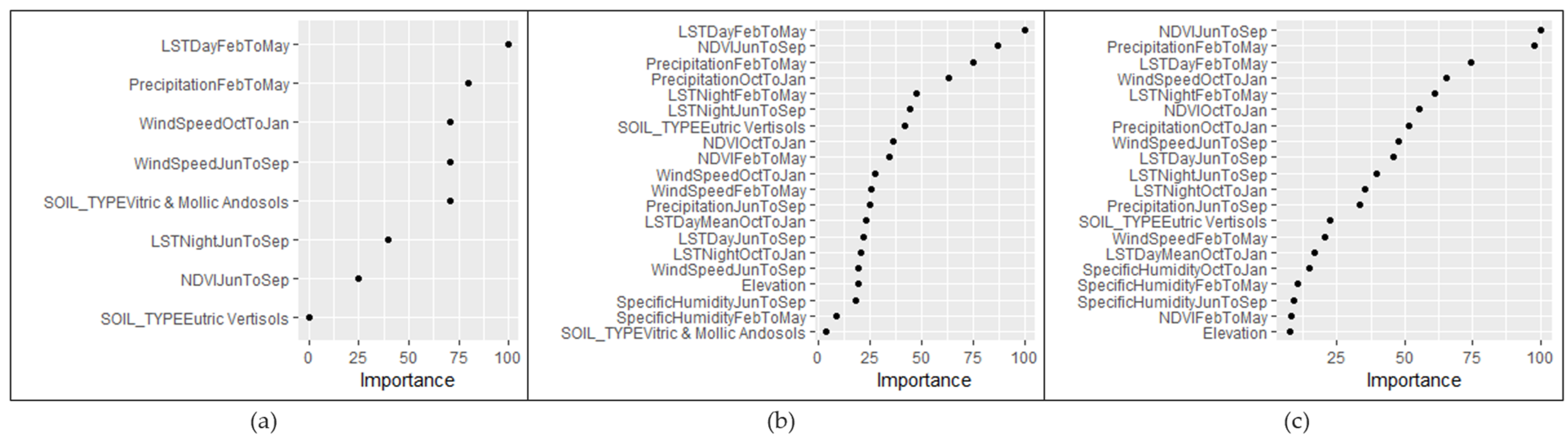
Figure 7 shows that the first three most important variables include LST daytime from Feb to May (X13), precipitation from Feb to May (X4), and wind speed from Oct to Jan (X9). Soil type (X2) eutric vertisols has an importance value of zero indicating that this predictor did not contribute to the predictive power of the model and was never used in any of the MARS basis functions in the pruned final model.
Even though MARS, being a nonparametric technique, does not assume linearity and homoscedasticity, the residual plot can still provide valuable diagnostic information about how well the model fits the data.
Figure 6 shows that the residuals are randomly scattered around zero, indicating that the variance of the error is approximately constant across all levels of the independent variables. This is a desirable property.
3.4. Artificial Neural Networks
The training of the ANN model was executed using the nnet and caret packages in R. The nnet package is designed to support a single hidden layer sandwiched between the input and output layers. In the preprocessing stage, the model is set to center and scale predictors, which is a common strategy to normalize variable scales.
Suited to regression tasks, the output layer of the neural network uses a linear activation function. The model incorporates key hyperparameters, such as weight decay for regularization, and the size, which determines the number of nodes in the hidden layer.
We set the range for ‘size’ from 1 to 10, and evaluated the ‘weight decay’ at 0, 0.01, and 0.1. After the tuning and training process, the model identified optimal hyperparameters: a decay value of 0.1 and a size of 10. A residual plot was generated to check the assumption of homoscedasticity. As shown in
Figure 6, the residuals were distributed randomly, suggesting that the assumption of the constant variance of errors is reasonable.
3.5. Random Forest Regression
The RFR model was trained using the randomForest package in R based on the training dataset, applying LOOCV as the resampling method. The hyperparameters for the RFR model included the number of randomly selected predictors at each split (mtry), the node size, and the number of trees (ntree). These hyperparameters were collectively tuned within a for loop. For mtry, a grid range of 1 to 10 was set and fine-tuned using the ‘caret’ package, whereas the node size was assessed at 5, 6, and 7, and the ntree parameter was evaluated between 50 and 200. Following this comprehensive grid search, the optimal settings were found to be an mtry value of 8, a node size of 5, and a ntree value of 60.
To assess the importance of the predictors, a variable importance plot was generated, revealing LST at daytime from Feb to May (X13), NDVI from Jun to Sep (X20), and precipitation from Feb to May (X4) to be of higher importance compared to the other variables, as depicted in
Figure 7.
In response to the inherent bias of the RFR model, as detailed in
Section 2.4.4, we employed a post-processing step to correct for this bias. This involved applying a linear transformation to the RFR predictions. Specifically, we fitted a linear regression model with the predicted water level from the initial RFR model as the independent variable and the actual water level as the dependent variable. The parameters of the transformation were estimated on the training sample. The estimated coefficients for the intercept (β0) and predicted water level variable (β
1) were −29.65 and 1.3, respectively. Comparing the residual plot for the original RFR model and the post-processed model, we see that the bias of the original RFR model has been mitigated.
3.6. Gradient Boosting Regression
GBR was constructed using gbm package in R. The hyperparameters such as the minimum number of observations in a node required for a split (n.minobsinnode), the boosting model’s complexity (interaction.depth), the number of iterations, and the learning rate were optimized via grid search. We assessed n.minobsinnode at values of 5 and 10, interaction.depth within a range of 1 to 3, iterations at 50, 70, 100, and 120, and learning rates at 0.1 and 0.01. The final optimal hyperparameters, which led to the best model performance, were 5, 2, 100, and 0.1, respectively.
To evaluate the importance of the predictors, a variable importance plot was generated, revealing NDVI from Jun to Sep (X20), precipitation from Feb to May (x4), and LST at daytime from Feb to May (X13) to be of higher importance compared to the other variables, as depicted in
Figure 7.
4. Discussion
4.1. Important Variables Analysis
In our study, we assessed variable importance using methods such as MI, significance of predictors through MLR, and GCV-based importance scoring for the MARS, RFR, and GBR models. While ANNs can be powerful predictors, they are not typically preferred for identifying important variables due to their ‘black box’ nature, which complicates the interpretation of individual feature contributions. Therefore, we did not assess variable importance for the ANN model.
The results of the variable importance analysis for each method were presented in
Section 3. Collectively, the findings suggest that three variables, namely, LST at daytime from February to May (X13), NDVI from June to September (X20), and precipitation from February to May (X4), consistently show strong importance across different models. Previous research also highlights temperature [
56], precipitation [
56,
57,
58], and NDVI [
59,
60] as primary factors influencing groundwater levels.
Some inconsistencies are observed between the analysis and the importance values from the machine learning models. This may stem from their differing methodological approaches to examining variable importance. Mutual information is a non-parametric method that quantifies the degree of dependence or relatedness between two variables. It can capture both linear and non-linear relationships, but it does not account for interactions between variables. Therefore, a variable might be rated as less important in mutual information analysis but may prove critical in a model where interactions between variables are considered. Machine learning models like MARS, RFR, and GBR not only consider individual variables’ contributions but also consider the interactions and combinations of variables. Consequently, these models can identify variables as important even if their individual relationships with the outcome variable are not strong, provided their combined effect with other variables is substantial. This highlights the importance of applying diverse methods when investigating variable importance. Each method brings its own strengths and can offer unique insights. Mutual information can identify variables that have a strong individual effect, whereas machine learning models can capture complex interaction effects.
4.2. Model Performance Evaluation and Comparison
As previously highlighted in
Section 2.2, multiple experiments were carried out for each machine learning algorithm. For the residual plots (
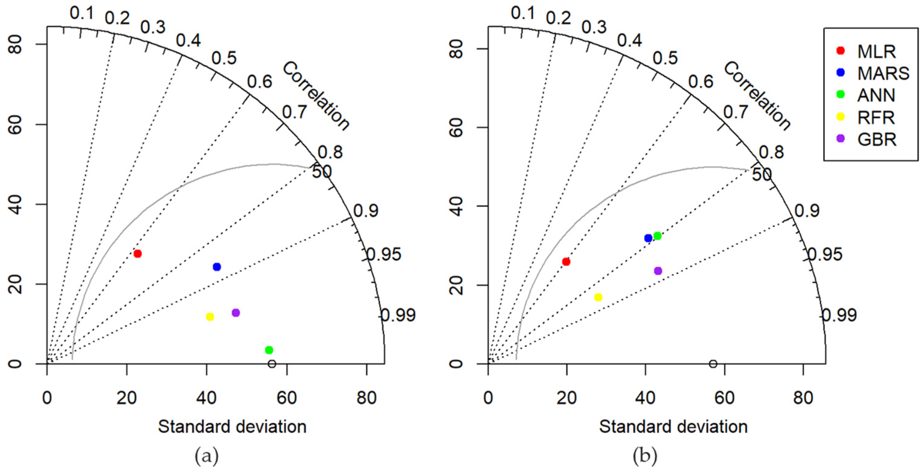
Figure 6), observed versus predicted plot (
Figure 8), Taylor diagram (
Figure 9), and the comparison in
Table 4, we selected a model with close to median performance across all models. To provide a more comprehensive understanding of each model’s performance, we also calculated the average performance score from the fifteen experiments. These averages are presented in
Table 5.
The results presented in
Table 4 show that GBR outperforms the other models with a high R-squared value of 0.76. In the Taylor diagram (
Figure 9b), the point representing GBR on the testing dataset is closer to the observed point on the
x-axis compared to other models, indicating a higher similarity in standard deviation between the GBR model output and the observations. While the performance of the RFR with linear transformation is slightly inferior to the GBR, it still outperforms the remaining models. This observation aligns with literature findings [
61,
62,
63], wherein gradient boosting consistently emerges as the top performer among the machine learning models used for water level predictions. In contrast, MLR appears insufficient for modeling our data effectively. The MARS model exhibits some predictive capability, though it does not fully capture the data’s complexity. With an R-squared value of 0.99 on the training data and 0.61 on the testing data, the ANN model shows clear evidence of overfitting to the training data. This occurs despite the model having a only single hidden layer and parameters that have been optimally tuned to avoid overfitting. The overfitting may stem from the small and potentially less diverse dataset, causing the model to memorize training data rather than learn to generalize from it. Future work might resolve this by enriching the dataset and/or simplifying the model.
Table 5 presents the average performance score based on multiple experiments conducted for each model. Consistent with the findings from the single experiment (
Table 4), GBR has the best performance among the models. The RFR model’s performance is slightly lower than that of GBR. MARS, on the other hand, exhibits the weakest average performance among the five models. Collectively, these results suggest that GBR and RFR are most suitable for predicting depth to water table for our data set, aligning with findings from previous research [
7,
15,
61,
62,
63].
It is worthy of note that other studies in the literature achieved better model performance than the results reported here, but these studies were based on time series data. When groundwater levels from a previous time period are available as a predictor, it is natural that predictions will be more accurate. We have not found other studies using machine learning to predict groundwater level in which no data on prior groundwater levels was available. For purposes of guiding drilling decisions, the ability to predict groundwater levels from publicly available hydrogeological and climate data, without the use of prior groundwater levels, is essential.
4.3. Grid Points Prediction Evaluation Based on the Best Model
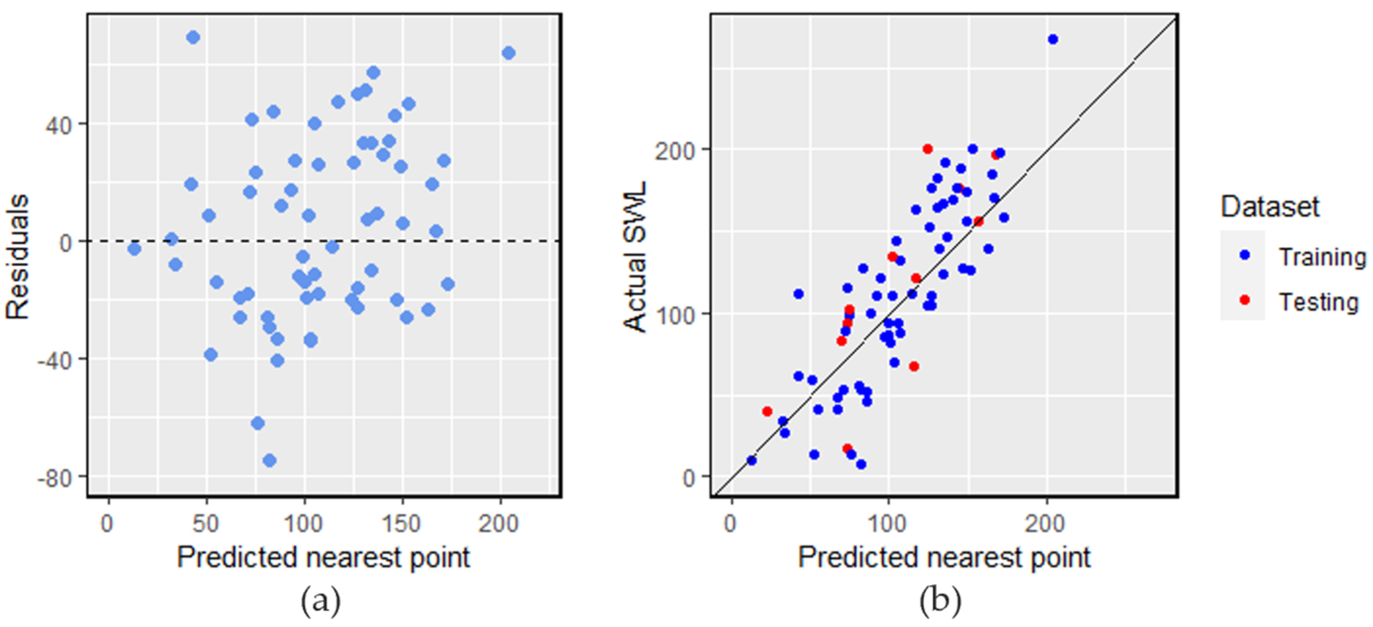
As detailed in
Section 2.2, the grid points were generated to comprehensively represent the study area. We utilized the primary GBR model presented in this paper (
Table 4) to generate predictions for these grid points. Given the map’s discretized nature, we evaluated prediction performance solely based on these grid points. This involved comparing the observed water levels from the existing 75 boreholes with the predicted water levels for their closest respective grid points (
Figure 10).
Table 6 illustrates the evaluation of water level predictions. It is worth noting that the predicted water levels are slightly worse on both the training and testing data in comparison to the performance reported in
Section 4.2. This is to be expected: it is naturally more accurate to predict based on predictor variables at the well location rather than based on predictor variables some distance away. However, this analysis shows that our model can be useful even if, as may be the case in practice, predictor values are available only at grid points and not at a specific well location. Thus, despite the slight drop in prediction accuracy, model results can still be valuable to support decisions about drilling locations in the region. While we have not seen such comparisons reported previously in the literature, we argue that comparing grid point predictions with their nearest actual measurements offers practical insights for drilling decisions.
4.4. Final Map of the Predicted Water Level
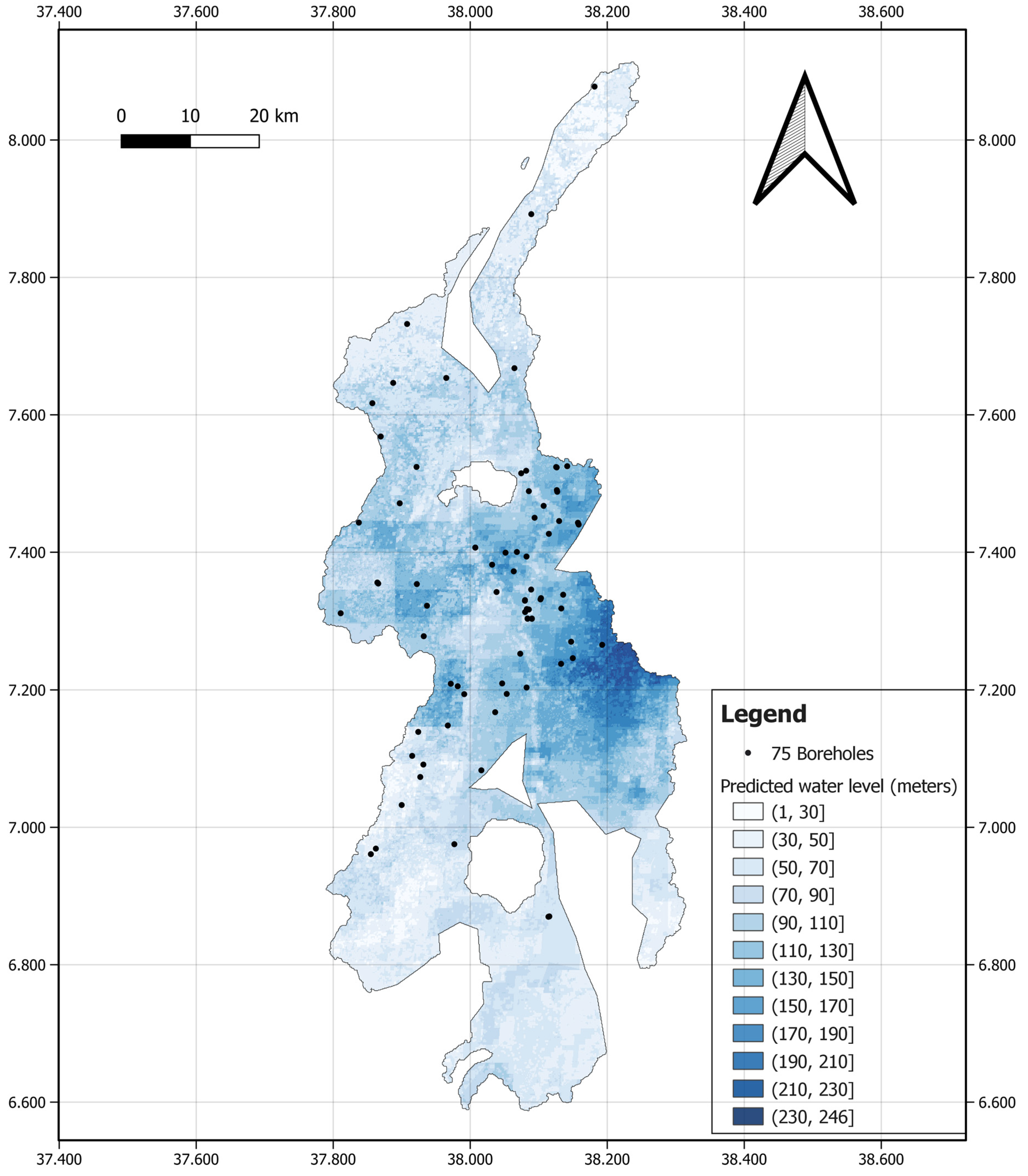
Utilizing QGIS, we generated a 100 m × 100 m resolution map based on the grid points (
Figure 11). The predicted groundwater levels of the grid points were broken into 20 m categories, and we color-coded the figure for the purpose of display. The regular block pattern in some areas of the map is due to the low resolution of some of the predictor variables. The map suggests that areas of shallow groundwater (under 30 m) are predominantly located in the northern and southern regions, with some patches in the central area. Conversely, the eastern region mostly features deeper groundwater. We found no previous studies specifically targeting the Bilate region for groundwater level predictions. A prior investigation assessed groundwater potential in Bilate using integrated GIS and remote sensing techniques [
64]. While a direct comparison between that study and ours is challenging due to differing objectives and methodologies, it is noteworthy that Gintamo [
64] identified the Middle Eastern part of the region as having low groundwater potential. This observation is consistent with our findings, where the predicted groundwater level in the middle eastern region is among the deepest. This high-resolution map can serve as a practical guide for borehole drilling for sustainable irrigation, particularly beneficial for stakeholders such as drilling companies, government entities, and local farmers.
5. Conclusions
Our research demonstrates the applicability of AI to identifying viable drilling sites for sustainable irrigation and drinking water in water-deficient areas. Prior studies have typically utilized time series data for groundwater level prediction. However, the challenge in water scarcity regions lies in the lack of data due to formidable data collection constraints. These regions, marked by higher water demand, necessitate effective strategies for groundwater exploitation.
Addressing this gap, we have utilized available non-time series data to construct and evaluate five machine learning models for groundwater level prediction. Of these, Gradient Boosting Regression consistently demonstrated superior performance, with an average R-squared value of 0.77 and an average median absolute error of 19 m across numerous experiments. The highest-performing model was subsequently employed to predict groundwater levels across the entire Bilate region. This process resulted in the development of a high-resolution map, anticipated to guide local communities and organizations in pinpointing the most suitable locations for sustainable irrigation drilling. Furthermore, these findings have the potential to enhance food security by providing valuable insights and guiding more informed agricultural and water resource management decisions.
Land Surface Temperature during daytime from February to May, NDVI from June to September, and precipitation from February to May consistently demonstrated importance across models. There were inconsistencies between the variable importance from the MI method and the machine learning methods. The results of these approaches should be considered complementary rather than contradictory. Using a combination of methods allows for a more robust and comprehensive understanding of variable importance, leading to a more reliable model. In case of substantial discrepancies, deeper investigations can be conducted to reconcile the findings.
There are some limitations of this study. Firstly, a potential concern is the relatively small dataset of 75 boreholes, which are not evenly distributed throughout the Bilate watershed. This may present a limitation for making region-wide predictions. Secondly, the predictor variables we considered were limited to ones that could be readily computed from publicly available data. Thirdly, the ANN model showed a tendency to overfit the training data, indicating the need for more extensive hyperparameter tuning and model simplification. Lastly, our data, having been collected in 2007, may be somewhat dated. Efforts are underway to acquire more recent data to verify prediction accuracy. Future research in this region should aim to improve the predictive power of groundwater levels by considering additional predictor variables (e.g., distance to water and elevation above permanent streams), forecast groundwater recharge, and analyze the impacts of climate change. This will provide comprehensive guidance for decision-making related to borehole drilling.


 ,
, 


